Injectivity Conditions for STFT Phase Retrieval on ${\mathbb {Z}}$, ${\mathbb {Z}}_d$ and ${{\mathbb {R}}}^d$

Abstract

We study the phase retrieval problem for the short-time Fourier transform on the groups ${\mathbb {Z}}$, ${\mathbb {Z}}_d$ and ${{\mathbb {R}}}^d$. As is well-known, phase retrieval is possible once the windows’s ambiguity function vanishes nowhere. However, there are only few results for windows that fail to meet this condition. The goal of this paper is to establish new and complete characterizations for phase retrieval with more general windows and compare them to existing results. For a fixed window, our uniqueness conditions usually only depend on the signal’s support and are therefore easily comprehensible. In the discrete settings, we also provide examples which show that a non-vanishing ambiguity function is not necessary for a window to do phase retrieval.

1 Introduction

We are interested in the phase retrieval problem for the short-time Fourier transform (STFT) on ${\mathbb {Z}}$, ${\mathbb {Z}}_d$ and ${{\mathbb {R}}}^d$. More precisely, we try to investigate whether a signal $f\in L^2(G)$ is uniquely determined (up to a global phase factor) by the measurement $|V_gf|$, where $g\in L^2(G)$ is a known window and $G\in \{{\mathbb {Z}},{\mathbb {Z}}_d,{{\mathbb {R}}}^d\}$. Here, the STFT is defined by

$$\begin{aligned} V_gf(k,z)&=\sum \limits _{j\in {\mathbb {Z}}} f_j\overline{g_{j-k}}z^{-j}\quad \quad (k\in {\mathbb {Z}},z\in {{\mathbb {C}}},|z|=1), \end{aligned}$$

(1)

$$\begin{aligned} V_gf(k,l)&=\sum \limits _{j=0}^{d-1} f_j\overline{g_{j-k}}e^{\nicefrac {-2\pi ijl}{d}}\quad \quad (k,l\in \{0,\dots ,d-1\})\quad \text {or} \end{aligned}$$

(2)

$$\begin{aligned} V_gf(x,\omega )&=\int \limits _{{{\mathbb {R}}}^d}^{}f(t)\overline{g(t-x)}e^{-2\pi i\langle t,\omega \rangle }~\textrm{d}t\quad \quad (x,\omega \in {{\mathbb {R}}}^d) \end{aligned}$$

(3)

for elements f and g of $\ell ^2({\mathbb {Z}})$, ${{\mathbb {C}}}^d$ or $L^2({{\mathbb {R}}}^d)$ respectively.

Applications of this specific phase retrieval problem include speech processing [12] and ptychography [10]. For a more general overview of phase retrieval and its applications, we refer the interested reader to the review paper [15].

For a fixed window g, the goal of this paper is to determine which signals f can be recovered from the measurement $|V_gf|$ (up to global phase). The common ground among all our results is that they are quite easy to understand since they usually only involve elementary connectedness conditions on the signal’s support.

It is already well-known that disconnectedness causes non-trivial ambiguities or at least instabilities for phase retrieval, both in the discrete [5, 11, 21, 23] and the continuous setting [4, 16]. There are also converse statements, i.e., assumptions on connectedness that lead to uniqueness results, most notably [5, Corollary 2.5] (see Theorem 2.2.3 below). However, uniqueness for STFT phase retrieval is still far from being completely understood.

The main tool in our approach is the observation that the given phase retrieval problem essentially reduces to the analysis of the so-called ambiguity functions $V_ff$ and $V_gg$. More precisely, it is crucial to determine whether the signal f can be recovered from the restriction of $V_ff$ to the support of $V_gg$.

This is one of the most prominent insights into STFT phase retrieval and has the well-known consequence that all signals can be uniquely recovered (up to global phase) once the window’s ambiguity function vanishes nowhere [8, 15, 16].

The so-called ambiguity function relation (see equation (4) below) has also been used in a more direct way in [6] in order to analyze phase retrieval for windows whose ambiguity functions potentially have much smaller supports. Here, the authors have proven uniqueness for bandlimited signals for the case of windows that are non-vanishing only on one or two line segments. In contrast, we usually consider larger signal classes, which (sometimes) comes at the cost of having to be slightly more restrictive on the window.

Finally, note that similar results can also be obtained using different proof methods, e.g., for the discrete setting in [8, Theorem 2.4] by application of the so-called PhaseLift operator.

1.1 Structure of the Paper

The paper is organized as follows: In Sect. 2, we recall some common tools for STFT phase retrieval which can be applied uniformly among the various settings.

After that, we specify to the three settings of interest (i.e., ${\mathbb {Z}}$, ${\mathbb {Z}}_d$ and ${{\mathbb {R}}}^d$) in Sects. 3, 4 and 5 respectively. Phase retrieval on ${\mathbb {Z}}$ is by far the easiest of the three. Using standard methods from complex analysis, we provide a full characterization of phase retrieval for windows that are either one-sided or of exponential decay (Theorem 3.1.7).

For the finite-dimensional setting (i.e., in ${\mathbb {Z}}_d$), we first examine whether a non-vanishing ambiguity function of the window is a necessary condition for (global) phase retrieval, which we prove to be false in every dimension $d\ge 4$ (Corollary 4.1.7). Afterwards, we restrict ourselves to short windows and prove a uniqueness result for a certain class of sparse signals (Theorem 4.2.8).

For the continuous setting (i.e., in ${{\mathbb {R}}}^d$), we face an additional challenge. While the ambiguity function can be controlled when making certain assumptions on the window, the recovery of the signal cannot be performed as easily as within the discrete settings since most of the information has to be understood in an “almost everywhere” sense. Again, we find a complete characterization of phase retrieval for one-sided windows (in dimension one) and for windows of exponential decay (Theorem 5.1.8). In contrast to the discrete setting, the proof involves a fair amount of measure theory. Finally, we apply our characterization to some examples (Sect. 5.4), including compactly supported windows.

1.2 Notation

We conclude this section by fixing some basic notation.

For $d\ge 2$, let ${\mathbb {Z}}_d:={\mathbb {Z}}/d{\mathbb {Z}}$ be the cyclic group of order d. We usually consider $d\in {\mathbb {N}}$ in order to treat the group ${{\mathbb {R}}}^d$ simultaneously. Note however that we always assume implicitly that $d\ge 2$ whenever considering ${\mathbb {Z}}_d$. We frequently identify ${\mathbb {Z}}_d\cong \{0,\dots ,d-1\}$ and accordingly write $x\in L^2({\mathbb {Z}}_d)\cong {{\mathbb {C}}}^d$ as $x=(x_0,\dots ,x_{d-1})^t$. However, we still think of $x\in L^2({\mathbb {Z}}_d)$ as a d-periodic signal, such that the evaluation $x_j$ is well-defined for every $j\in {\mathbb {Z}}$.

For $p\ge 1$, with a slight abuse of notation, we always think of $f\in L^p\left( {{\mathbb {R}}}^d\right)$ as a measurable, p-integrable function $f:{{\mathbb {R}}}^d\rightarrow {{\mathbb {C}}}$. On ${{\mathbb {C}}}^d$, $\ell ^2({\mathbb {Z}})$ and $L^2\left( {{\mathbb {R}}}^d\right)$, we choose the standard inner products

for $x,y\in {{\mathbb {C}}}^d$, $a,b\in \ell ^2({\mathbb {Z}})$ and $f,g\in L^2({{\mathbb {R}}}^d)$ respectively.

We let ${\mathbb {T}}:=\{z\in {{\mathbb {C}}}~|~|z|=1\}$ be the torus and define the Fourier transform of $x\in {{\mathbb {C}}}^d$, $a\in \ell ^1({\mathbb {Z}})$ and $f\in L^1({{\mathbb {R}}}^d)$, evaluated at $0\le l\le d-1$, $z\in {\mathbb {T}}$ and $\omega \in {{\mathbb {R}}}^d$ respectively by

$$\begin{aligned}{} & {} ({\mathcal {F}}_{{\mathbb {Z}}_d}x)_l:=\sum _{j=0}^{d-1} x_je^{\nicefrac {-2\pi ijl}{d}},\quad ({\mathcal {F}}_{{\mathbb {Z}}}a)(z):=\sum _{j\in {\mathbb {Z}}} a_j z^{-j}\quad \text {and}\\ {}{} & {} \quad ({\mathcal {F}}_{{{\mathbb {R}}}^d}f)(\omega ):=\int _{{{\mathbb {R}}}^d} f(t)e^{-2\pi i\langle t,\omega \rangle }\textrm{d}t \end{aligned}$$

and omit the subscript whenever it is clear from the context or when treating multiple settings simultaneously. For $k\in {\mathbb {Z}}$, we define the translation operator by $(T_k x)_j=x_{j-k}$ for both $x\in {{\mathbb {C}}}^d$ and $x\in {{\mathbb {C}}}^{{\mathbb {Z}}}$. Analogously, we let $(T_t f)(x)=f(x-t)$ for all $t\in {{\mathbb {R}}}^d$ and all measurable functions $f:{{\mathbb {R}}}^d\rightarrow {{\mathbb {C}}}$. We use the notation $\text {supp}(x)$ to denote the support of $x\in {{\mathbb {C}}}^d$ or $x\in {{\mathbb {C}}}^{{\mathbb {Z}}}$ as well as $\text {supp}(f)$ to denote the essential support of $f\in L^2({{\mathbb {R}}}^d)$, i.e., the intersection of all closed sets $A\subseteq {{\mathbb {R}}}^d$ satisfying $f\vert _{A^c}\equiv 0$ almost everywhere. In particular, $\text {supp}(f)$ is closed and we have $\text {supp}(f)=\text {supp}(h)$ whenever f and h agree almost everywhere. It is also easy to show that in fact, $f\equiv 0$ holds almost everywhere on ${{\mathbb {R}}}^d\setminus \text {supp}(f)$. For $G\in \{{\mathbb {Z}}_d,{\mathbb {Z}}\}$ and $z\in G$, we define $\delta _z:G\rightarrow {{\mathbb {C}}}$ to equal the characteristic function $\chi _{\{z\}}$.

For $r>0$, $z_0\in {{\mathbb {C}}}$ and $x_0\in {{\mathbb {R}}}^d$, we define the disk $K_r(z_0):=\{z\in {{\mathbb {C}}}~|~|z-z_0|<r\}$ as well as the ball $B_r(x_0):=\{x\in {{\mathbb {R}}}^d~|~\Vert x-x_0\Vert _{\infty }<r\}$. Additionally, we define the annulus $A_r(z_0):=\{z\in {{\mathbb {C}}}~|~r^{-1}<|z-z_0|<r\}$ when $r>1$.

Finally, we let denote the Lebesgue measure on ${{\mathbb {R}}}^d$ and for two measurable sets $A,B\subseteq {{\mathbb {R}}}^d$, we say that A has full measure in B iff .

2 Fundamentals of STFT Phase Retrieval

The goal of this section is to collect some common tools for STFT phase retrieval. In order to treat the three settings of interest uniformly, let $G\in \{{\mathbb {Z}},{\mathbb {Z}}_d,{{\mathbb {R}}}_d\}$. We let ${\widehat{G}}$ denote the dual group of G which is given by ${\widehat{{\mathbb {Z}}}}={\mathbb {T}}$, $\widehat{{\mathbb {Z}}_d}={\mathbb {Z}}_d$ and $\widehat{{{\mathbb {R}}}^d}={{\mathbb {R}}}^d$ respectively. The short-time Fourier transform of a signal $f\in L^2(G)$ with respect to a window $g\in L^2(G)$ is then defined by

$$\begin{aligned} V_gf(x,\omega )={\mathcal {F}}\left( f\cdot \overline{T_x g}\right) (\omega ) \end{aligned}$$

for all $x\in G, \omega \in {\widehat{G}}$, which results in the explicit formulae (1)–(3).

2.1 The Phase Retrieval Problem

For fixed g, the phase retrieval problem associated with the STFT tries to recover a signal f from the phaseless measurement $|V_gf|$. Since the STFT is linear in f, we immediately obtain $|V_gf|=|V_g(\gamma f)|$ for every $\gamma \in {\mathbb {T}}$. Thus, there is only a chance to recover f up to a global phase factor. With that in mind, we call f phase retrievable w.r.t. g iff the statement

$$\begin{aligned} \left| V_g f\right| =\left| V_g {\tilde{f}}\right| \quad \Rightarrow \quad {\tilde{f}}=\gamma f~\text {for some }\gamma \in {\mathbb {T}}\end{aligned}$$

holds true for every ${\tilde{f}}\in L^2(G)$.

We say that the window g does phase retrieval iff every $f\in L^2(G)$ is phase retrievable w.r.t. g.

Remark 2.1.1

For $y\in G$, it follows immediately from the definition that f is phase retrievable w.r.t. g if and only if it is phase retrievable w.r.t. $T_y g$. Letting $({\mathcal {I}}h)(x):=h(-x)$ for all $h\in L^2(G)$ and $x\in G$, this is also equivalent to ${\mathcal {I}}f$ being phase retrievable w.r.t. ${\mathcal {I}}g$.

A common approach for phase retrieval is based on the so-called ambiguity function relation

$$\begin{aligned} {\mathcal {F}}\left( \left| V_gf\right| ^2\right) (\omega ,x)=c_G\cdot V_ff(-x,\omega )\cdot \overline{V_gg(-x,\omega )} \end{aligned}$$

(4)

which holds for all $(x,\omega )\in G\times {\widehat{G}}$ [6, 15, 16]. Here, $c_G>0$ denotes a constant and ${\mathcal {F}}$ denotes the Plancherel transform on the product $G\times {\widehat{G}}$. Note that the term on the left-hand side is well-defined since $|V_gf|\in L^2(G\times {\widehat{G}})$ [13]. Additionally, we have $c_G=1$ when $G\in \{{\mathbb {Z}},{{\mathbb {R}}}^d\}$ and $c_G=d$ when $G={\mathbb {Z}}_d$. Directly from the definition of the STFT, we can also derive the symmetry relations

$$\begin{aligned} \begin{aligned} V_hh(-k,z^{-1})&=z^{-k}\cdot \overline{V_hh(k,z)},\\ V_hh(-k,-l)&=e^{\nicefrac {-2\pi ikl}{d}}\cdot \overline{V_hh(k,l)}\qquad \text {and}\\ V_hh(-x,-\omega )&=e^{-2\pi i \langle x,\omega \rangle }\cdot \overline{V_hh(x,\omega )} \end{aligned} \end{aligned}$$

(5)

for $h\in \ell ^2({\mathbb {Z}})$, $h\in {{\mathbb {C}}}^d$ or $h\in L^2({{\mathbb {R}}}^d)$ respectively.

Remark 2.1.2

When $G={{\mathbb {R}}}^d$, the function $(x,\omega )\mapsto e^{\pi i x\omega } V_hh(x,\omega )$ is usually referred to as the ambiguity function of a signal $h\in L^2({{\mathbb {R}}}^d)$. However, in order to introduce a coherent terminology between the various settings, we use the term “ambiguity function” for the non-modulated version $V_h h$ where $h\in L^2(G)$.

Using the notation

$$\begin{aligned} \Omega _g:=\left\{ (x,\omega )\in G\times {\widehat{G}}~\big |~V_gg(x,\omega )\ne 0\right\} \end{aligned}$$

for $g\in L^2(G)$, equation (4) implies the following lemma.

Lemma 2.1.3

A signal $f\in L^2(G)$ is phase retrievable w.r.t. a window $g\in L^2(G)$ if and only if the statement

$$\begin{aligned} V_ff\vert _{\Omega _g}=V_{{\tilde{f}}}{\tilde{f}}\vert _{\Omega _g}\quad \Rightarrow \quad {\tilde{f}}=\gamma f\text { almost everywhere for some } \gamma \in {\mathbb {T}}\end{aligned}$$

holds true for every ${\tilde{f}}\in L^2(G)$.

Since it is well-known that the full ambiguity function $V_ff$ determines f up to a global phase factor, we obtain the following theorem [8, 15, 16].

Theorem 2.1.4

Let $g\in L^2(G)$ and suppose that $\Omega _g$ is a set of full measure in $G\times {\widehat{G}}$. Then, g does phase retrieval.

Even for windows which do not satisfy the assumption of Theorem (2.1.4), we can use Lemma (2.1.3) in order to deduce phase retrieval results along the following steps:

• (1) Provide conditions on a window g that allow to characterize the corresponding set $\Omega _g$.

• (2) Based on the knowledge of $\Omega _g$, provide conditions on a signal f that allow to decide whether f is phase retrievable w.r.t. g.

This strategy has previously been used in [6], where the authors provide uniqueness results for bandlimited signals requiring only mild conditions on the window.

In this paper, we intend to formulate the conditions in (1) and (2) mostly in terms of the supports of f and g in order for the ensuing results to be easily understandable.

Remark 2.1.5

Note that the results stated in this subsection can also be formulated on general $\sigma$-compact, metrizable LCA groups by using Fourier analysis on groups [26].

2.2 Phase Retrieval and Connectedness

It is a well-known fact [4, 5, 11, 16, 21, 23] that phase retrieval crucially depends on certain types of connectedness of the signal. The goal of this paper is to provide uniqueness results for phase retrieval that revolve around this observation. In this subsection, we outline the principal idea, which has already featured prominently in [5, 15, 23].

Fix a window g and assume that $x\in G$ is such that $(x,\omega )\in \Omega _g$ holds for almost every $\omega \in {\widehat{G}}$. By Lemma 2.1.3 and the injectivity of the Fourier transform, we may then use the function $f\cdot \overline{T_xf}$ for the recovery of the signal f. Specifically for $x=0$, this corresponds to $|f|^2$. When G is discrete (i.e., $G\in \{{\mathbb {Z}},{\mathbb {Z}}_d\}$), phase retrieval may then (intuitively) be performed using the following two steps.

• (1) Fix a phase for f at some $y\in G$ satisfying $f(y)\ne 0$.

• (2) Propagate the phase along G using the information about $f\cdot \overline{T_x f}$ for various $x\ne 0$.

Obviously, we will lose the phase information when coming across zeros of f within step (2). At this point, the role of connectedness becomes evident. Let us make this more precise by considering the set $D_g:=\left\{ x\in G~|~g\cdot \overline{T_x g}\not \equiv 0\right\}$. Clearly, for $G\in \{{\mathbb {Z}},{\mathbb {Z}}_d\}$, it follows $D_g=\{y-z\,|\,y,z\in \text {supp}(g)\}$. For $G={{\mathbb {R}}}^d$, note that $0\in D_g$ holds true whenever $g\ne 0$. Additionally, continuity of $V_gg$ implies that $D_g$ is open. (At least for compactly supported g, this has also been observed in [18].) Now, we make the following definition.

Definition 2.2.1

Consider a subset $M\subseteq G$ as well as a signal $f\in L^2(G)$ and a window $g\in L^2(G)$.

• (a) Two elements $j,k\in M$ are called g-connected and we write $j\sim _g k$ iff there exist $l_0,\dots ,l_n\in M$ satisfying $l_0=j$, $l_n=k$ and $l_{m+1}-l_m\in D_g$ for every $0\le m<n$.

• (b) Clearly, $\sim _g$ defines an equivalence relation on M. The equivalence classes of M are called g-connected components of M and M is called g-connected iff there exists at most one g-connected component.

• (c) f is called g-connected iff ${\text {supp}}(f)$ is g-connected. The g-connected components of ${\text {supp}}(f)$ are called g-connected components of f.

With this definition, we immediately obtain the following necessary condition for phase retrieval.

Lemma 2.2.2

Let $f,{\tilde{f}},g\in L^2(G)$ and let $\left( C_m\right) _{m\in I}$ be the g-connected components of f.

• (a) If $\text {supp}\left( {\tilde{f}}\right) =\text {supp}(f)$ holds true and if for every $m\in I$, there exists $\gamma _m\in {\mathbb {T}}$ satisfying ${\tilde{f}}\vert _{C_m}=\gamma _m f\vert _{C_m}$ almost everywhere, then $\left| V_g{\tilde{f}}\right| =|V_gf|$.

• (b) If f is phase retrievable w.r.t. g, then f is g-connected.

Proof

• (a) The given condition is a common way of creating counterexamples for phase retrieval [4, 11, 16, 23]: Consider $(x,\omega )\in \Omega _g$, which implies $x\in D_g$. For every $y\in G$, it follows that either at least one of the points y and $y-x$ is not in $\text {supp}(f)$ or that both points belong to the same connected component of $\text {supp}(f)$. This readily implies ${\tilde{f}}\cdot \overline{T_x{\tilde{f}}}=f\cdot \overline{T_x f}$ almost everywhere. Altogether, it follows $V_{{\tilde{f}}}{\tilde{f}}\vert _{\Omega _g}=V_ff\vert _{\Omega _g}$ and therefore $\left| V_g{\tilde{f}}\right| =|V_gf|$ by (4).

• (b) For $G\in \{{\mathbb {Z}},{\mathbb {Z}}_d\}$, the statement follows immediately from a). For $G={{\mathbb {R}}}^d$, it remains to show that every connected component is a set of positive measure. Assume $g\ne 0$, let $m\in I$ and pick $x\in C_m$. Since $D_g$ is open and satisfies $0\in D_g$, there exists an open neighborhood U of 0 satisfying $U\subseteq D_g$. Since $C_m\subseteq \text {supp}(f)$, it follows (by definition of the essential support) that $(U+x)\cap \text {supp}(f)$ is a set of positive measure. Now, $U\subseteq D_g$ implies $(U+x)\cap \text {supp}(f)=(U+x)\cap C_m$ and therefore, $C_m$ must be of positive measure.

$\square$

When $G\in \{{\mathbb {Z}},{\mathbb {Z}}_d\}$, there is also a converse statement under the assumption that $\Omega _g$ is a set of full measure in $D_g\times {\widehat{G}}$. The following theorem has appeared for the case $G={\mathbb {Z}}_d$ and $D_g=\{-L,\dots ,L\}$ for some $L\ge 0$ in [5, Corollary 2.5]. The proof for the general case is entirely analogous.

Theorem 2.2.3

Let $G\in \{{\mathbb {Z}},{\mathbb {Z}}_d\}$ as well as $f,g\in L^2(G)$. Assume that $\Omega _g$ is a set of full measure in $D_g\times {\widehat{G}}$ and let $(C_m)_{m\in I}$ be the g-connected components of f. Then, the following statements hold true.

• (a) A signal ${\tilde{f}}\in L^2(G)$ satisfies $\left| V_g f\right| =\left| V_g{\tilde{f}}\right|$ if and only if ${\text {supp}}\left( {\tilde{f}}\right) ={\text {supp}}(f)$ and for every $m\in I$, there exists $\gamma _m\in {\mathbb {T}}$ satisfying ${\tilde{f}}\vert _{C_m}=\gamma _mf\vert _{C_m}$.

• (b) f is phase retrievable w.r.t. g if and only if f is g-connected.

• (c) g does phase retrieval if and only if $D_g=G$.

The goal of Sects. 3 and 4 is to identify large window classes for which the assumptions of Theorem 2.2.3 are satisfied and provide sharp criteria for phase retrieval in cases where the assumptions are not satisfied. As a special instance, we answer the question whether $\Omega _g$ being of full measure in $G\times {\widehat{G}}$ is a necessary condition for global phase retrieval. In Sect. 5, we prove an analogue of Theorem 2.2.3 for a large window class in the case $G={{\mathbb {R}}}^d$.

3 STFT Phase Retrieval on ${\mathbb {Z}}$

In this section, we analyze phase retrieval on the group $G={\mathbb {Z}}$. Recall that in this setting, the STFT is given by

$$\begin{aligned} V_gf(k,z)=\sum \limits _{j\in {\mathbb {Z}}} f_j\overline{g_{j-k}}z^{-j}\quad (k\in {\mathbb {Z}},z\in {\mathbb {T}}). \end{aligned}$$

In Subsect. 3.1, we use Theorem 2.2.3 in order to prove a full characterization of phase retrieval for one-sided as well as exponentially decaying windows. In Subsect. 3.2, we provide an example of a window $g\in \ell ^2({\mathbb {Z}})$ doing phase retrieval despite the fact that $\Omega _g$ is not of full measure in ${\mathbb {Z}}\times {\mathbb {T}}$.

3.1 Uniqueness Conditions for Phase Retrieval on ${\mathbb {Z}}$

We begin by considering a finitely supported window $g\in \ell ^2({\mathbb {Z}})$. By Remark 2.1.1, we may assume w.l.o.g. that $\text {supp}(g)\subseteq \{0,\dots , L\}$ holds for some $L\in {\mathbb {N}}_0$. In this case, it follows

$$\begin{aligned} V_gg(k,{\overline{z}})=\sum \limits _{j=k}^L g_j\overline{g_{j-k}}z^j=z^k\cdot \sum \limits _{j=0}^{L-k}g_{j+k}\overline{g_j}z^j \end{aligned}$$

(6)

for all $z\in {\mathbb {T}}={\overline{{\mathbb {T}}}}$ and all $k\ge 0$. For every $k\ge 0$ satisfying $k\in D_g$, at least one coefficient of the polynomial $\sum _{j=0}^{L-k} g_{j+k}\overline{g_j} z^j$ is nonzero and thus, the polynomial can have at most $L-k$ zeros (on ${\mathbb {T}}$). By (5), it follows that g satisfies the assumption of Theorem 2.2.3.

Corollary 3.1.1

Let $g\in \ell ^2({\mathbb {Z}})$ be finitely supported. Then, $\Omega _g$ is a set of full measure in $D_g\times {\mathbb {T}}$.

In the case where $\text {supp}(g)=\{0,\dots ,L\}$, there is also an easy interpretation of connectedness: A signal $f\in \ell ^2({\mathbb {Z}})$ is g-connected iff its support is connected up to “holes” of length at most $L-1$.

As a generalization, we consider one-sided windows.

Definition 3.1.2

A window $g\in \ell ^2({\mathbb {Z}})$ is called one-sided if there exists $K\in {\mathbb {Z}}$ such that $g_j=0$ either holds for all $j\le K$ or for all $j\ge K$.

By Remark 2.1.1, we may assume w.l.o.g. that ${\text {supp}}(g)\subseteq {\mathbb {N}}_0$. Clearly, finitely supported windows are a special instance of one-sided windows. In the case of a one-sided window, we obtain

$$\begin{aligned} V_gg(k,{\overline{z}})=z^k\sum \limits _{j=0}^{\infty } g_{j+k}\overline{g_j}z^j \end{aligned}$$

for all $k\in {\mathbb {N}}_0$ and all $z\in {\mathbb {T}}$. Thus, we need to replace the polynomials from above by the power series

$$\begin{aligned} P_k(z):=\sum \limits _{j=0}^{\infty } g_{j+k}\overline{g_j}z^j. \end{aligned}$$

Clearly, $P_k$ does not vanish identically on $K_1(0)$ whenever $k\in D_g$.

If we could assume that $P_k$ converges on a slightly larger disk $K_r(0)$ for some $r>0$, it would define a holomorphic function on the larger disk and therefore allow only finitely many zeros on the compact set ${\mathbb {T}}$. Unfortunately, this assumption does not hold true in general. (Consider for instance $g_j:=\frac{1}{j}$.) However, we are still able to conclude that $P_k(z)\ne 0$ holds for almost every $z\in {\mathbb {T}}$. In order to do so, we need some theory on Hardy spaces provided in [25].

Lemma 3.1.3

Let $\left( c_j\right) _{j\in {\mathbb {N}}_0}\in \ell ^1\left( {\mathbb {N}}_0\right)$ and define

$$\begin{aligned} h(z):=\sum \limits _{j=0}^{\infty } c_jz^j \end{aligned}$$

for every $z\in \overline{K_1(0)}$. Furthermore, assume that $c_j\ne 0$ holds for some $j\in {\mathbb {N}}_0$. Then, $h(z)\ne 0$ holds for almost every $z\in {\mathbb {T}}$.

Proof

We use the notation from [25]. First, h does not vanish identically on $K_1(0)$ by assumption. Additionally, note that $\left( c_j\right) _{j\in {\mathbb {N}}}\in \ell ^1\left( {\mathbb {N}}_0\right) \subseteq \ell ^2\left( {\mathbb {N}}_0\right)$, which implies $h\vert _{K_1(0)}\in H^2$ by [25, Theorem 17.12]. Now, the claim follows by [25, Theorem 17.18]. $\square$

Combining Lemma 3.1.3 with (5) and the fact that $\left( g_{j+k}\overline{g_j}\right) _{j\in {\mathbb {N}}_0}\in \ell ^1({\mathbb {N}}_0)$ holds for every $k\in {\mathbb {N}}_0$, it follows that Corollary 3.1.1 generalizes to one-sided windows.

Corollary 3.1.4

Let $g\in \ell ^2({\mathbb {Z}})$ be one-sided. Then, $\Omega _g$ is a set of full measure in $D_g\times {\mathbb {T}}$.

Finally, we consider the case of a general window $g\in \ell ^2({\mathbb {Z}})$. Here, we have to replace the power series $P_k$ by Laurent series

$$\begin{aligned} L_k(z):=\sum \limits _{j\in {\mathbb {Z}}} g_{j+k}\overline{g_j}z^j. \end{aligned}$$

In this case, the theory of Hardy spaces is no longer applicable. However, we may use the initial idea to obtain a theorem that works under the assumption of slightly better convergence. Therefore, we consider windows of exponential decay.

Definition 3.1.5

A window $g\in \ell ^2({\mathbb {Z}})$ is said to be of exponential decay if the series

$$\begin{aligned} \sum _{j\in {\mathbb {Z}}} |g_j|^2 e^{\sigma \cdot |j|} \end{aligned}$$

(7)

converges for some $\sigma >0$.

Clearly, convergence of the series (7) implies convergence of the Laurent series $L_0(z)$ on the annulus $A_{e^{\sigma }}(0)$. Additionally, by writing $z=z_1z_2$ where $z_1:=|z|^{\nicefrac {1}{2}}$ and $z_2:=\frac{z}{z_1}$ and applying Hölder’s equality, convergence of $L_0(z)$ on $A_{e^{\sigma }}(0)$ already implies convergence of $L_k(z)$ on $A_{e^{\sigma }}(0)$ for every $k\in {\mathbb {Z}}$.

Accordingly, in the case of an exponentially decaying window, each $L_k$ defines a holomorphic function on some annulus containing ${\mathbb {T}}$ and can thus have at most finitely many zeros on ${\mathbb {T}}$ once $k\in D_g$.

Corollary 3.1.6

Let $g\in \ell ^2({\mathbb {Z}})$ be of exponential decay. Then, $\Omega _g$ is a set of full measure in $D_g\times {\mathbb {T}}$.

Combining Corollaries 3.1.4 and 3.1.6 with Theorem 2.2.3 yields the following characterization for phase retrieval.

Theorem 3.1.7

Let $g\in \ell ^2({\mathbb {Z}})$ be either one-sided or of exponential decay. Furthermore, consider a signal $f\in \ell ^2({\mathbb {Z}})$ and let $\left( C_m\right) _{m\in {\mathbb {N}}}$ be the g-connected components of f. Then, the following statements hold true.

• (a) A signal ${\tilde{f}}\in \ell ^2({\mathbb {Z}})$ satisfies $\left| V_gf\right| =\left| V_g{\tilde{f}}\right|$ if and only if ${\text {supp}}\left( {\tilde{f}}\right) ={\text {supp}}(f)$ and for every $m\in {\mathbb {N}}$, there exists $\gamma _m\in {\mathbb {T}}$ satisfying ${\tilde{f}}\vert _{C_m}=\gamma _mf\vert _{C_m}$.

• (b) f is phase retrievable w.r.t. g if and only if f is g-connected.

• (c) g does phase retrieval if and only if $D_g={\mathbb {Z}}$.

Letting $g^{(1)}_j:=\frac{1}{j}$ for $j\in {\mathbb {N}}$ and $g^{(1)}_j:=0$ for $j\le 0$ as well as $g^{(2)}_j:=2^{-|j|}$ for all $j\in {\mathbb {Z}}$, we obtain two straightforward examples of windows doing phase retrieval.

3.2 Necessary Conditions for Global Phase Retrieval

To conclude this section, we want to discuss whether $\Omega _g$ being of full measure in ${\mathbb {Z}}\times {\mathbb {T}}$ is not only a sufficient but also a necessary condition for g to do phase retrieval. For both one-sided and exponentially decaying windows, we have already seen that $\Omega _g$ is of full measure in $D_g\times {\mathbb {T}}$. Since $D_g={\mathbb {Z}}$ is necessary for phase retrieval, we obtain the following statement.

Corollary 3.2.1

Let $g\in \ell ^2({\mathbb {Z}})$ be either one-sided or of exponential decay. Then, g does phase retrieval if and only if $\Omega _g$ is a set of full measure in ${\mathbb {Z}}\times {\mathbb {T}}$.

For general windows, this statement is no longer true. In order to see this, we first state the following reconstruction result.

Theorem 3.2.2

Let $f,{\tilde{f}}\in \ell ^2({\mathbb {Z}})$ and suppose that there exists an index $k^{*}>0$ such that the following conditions hold true.

• (i) It holds $V_ff(0,z)=V_{{\tilde{f}}}{\tilde{f}}(0,z)$ for almost every $z\in {\mathbb {T}}$.

• (ii) For every $k>k^{*}$, it holds $V_ff(k,z)=V_{{\tilde{f}}}{\tilde{f}}(k,z)$ for almost every $z\in {\mathbb {T}}$.

• (iii) It holds $|Z(k)|\ge 2k^{*}-k+1$ for every $0<k\le k^{*}$ where

  $$\begin{aligned} Z(k):=\left\{ z\in {\mathbb {T}}~\big |~V_ff(k,z)=V_{{\tilde{f}}}{\tilde{f}}(k,z)\right\} . \end{aligned}$$

Then, there exists $\gamma \in {\mathbb {T}}$ satisfying ${\tilde{f}}=\gamma f$.

Proof

W.l.o.g. assume $f\not \equiv 0$. From (i) and (ii), we obtain $|f|=\left| {\tilde{f}}\right|$ as well as $f\cdot \overline{T_k f}={\tilde{f}}\cdot \overline{T_k{\tilde{f}}}$ for every $k>k^{*}$ by Fourier inversion.

In the case where there exist $j_0,j_1\in \text {supp}(f)=\text {supp}\left( {\tilde{f}}\right)$ satisfying $j_1-j_0\ge 2k^{*}+1$, we fix $\gamma :=\frac{{\tilde{f}}_{j_0}}{f_{j_0}}$. This implies ${\tilde{f}}_j=\gamma f_j$ for every $j\ge j_0+k^{*}+1$ and in particular ${\tilde{f}}_{j_1}=\gamma f_{j_1}$. From the latter, we obtain ${\tilde{f}}_j=\gamma f_j$ for every $j\le j_1-k^{*}-1$ and since $j_1-k^{*}-1\ge j_0+k^{*}$ holds by assumption, it follows ${\tilde{f}}=\gamma f$.

Otherwise, assume w.l.o.g. that ${\text {supp}}(f)={\text {supp}}\left( {\tilde{f}}\right) \subseteq \{0,\dots ,2k^{*}\}$. As in (6), there exist polynomials $Q_k$ and ${\widetilde{Q}}_k$ of degree $2k^{*}-k$ satisfying

$$\begin{aligned} V_ff(k,{\overline{z}})=z^k\cdot Q_k(z)\quad \text {and}\quad V_{{\tilde{f}}}{\tilde{f}}(k,{\overline{z}})=z^k\cdot {\widetilde{Q}}_k(z) \end{aligned}$$

for all $0<k\le k^{*}$ and all $z\in {\mathbb {T}}$. By (iii), $Q_k$ and ${\widetilde{Q}}_k$ agree on a set of $2k^{*}-k+1$ elements, which implies in turn that $V_ff(k,\cdot )$ and $V_{{\tilde{f}}}{\tilde{f}}(k,\cdot )$ agree on ${\mathbb {T}}$. Together with (i), (ii) and (5), we obtain that $V_ff$ and $V_{{\tilde{f}}}{\tilde{f}}$ agree (almost) everywhere, which implies ${\tilde{f}}=\gamma f$ for some $\gamma \in {\mathbb {T}}$. $\square$

Theorem 3.2.2 yields the following phase retrieval result.

Corollary 3.2.3

Let $g\in \ell ^2({\mathbb {Z}})$ be such that $D_g={\mathbb {Z}}$ Furthermore, assume that there exists $k^{*}\in {\mathbb {N}}$ such that the set $\Omega _{g,k}:=\{z\in {\mathbb {T}}~|~(k,z)\in \Omega _g\}$ is of full measure in ${\mathbb {T}}$ whenever $k=0$ or $k>k^{*}$. Then, g does phase retrieval.

Proof

For $0<k\le k^{*}$, the fact that $k\in D_g$ implies $\Omega _{g,k}\ne \emptyset$. By continuity of $V_gg$, it follows that the set $\Omega _{g,k}$ is infinite. In particular, whenever $f,{\tilde{f}}\in \ell ^2({\mathbb {Z}})$ satisfy $V_ff\vert _{\Omega _g}=V_{{\tilde{f}}}{\tilde{f}}\vert _{\Omega _g}$, the assumptions of Theorem 3.2.2 are satisfied and it follows ${\tilde{f}}=\gamma f$ for some $\gamma \in {\mathbb {T}}$. By Lemma 2.1.3, g does phase retrieval. $\square$

Now we are ready to give an example of a window g doing phase retrieval despite $\Omega _g$ not being of full measure in ${\mathbb {Z}}\times {\mathbb {T}}$.

Example 3.2.4

Let $g\in \ell ^2({\mathbb {Z}})$ be given by

$$\begin{aligned} g_j:={\left\{ \begin{array}{ll} \frac{(-1)^k}{\sqrt{\pi }}\cdot \frac{1}{j+1}&{}\text {if } j=2k \text { for some } k\in {\mathbb {Z}},\\ \frac{i}{4}&{}\text {if } j\in \{1,-3\},\\ 1&{}\text {if } j=-1,\\ 0&{}\text {otherwise}.\end{array}\right. } \end{aligned}$$

Then, the following statements hold true.

• (a) It holds $V_gg(2,z)=0$ for every $z\in {\mathbb {T}}$ satisfying ${\text {Im}}(z)<0$.

• (b) g does phase retrieval.

Proof

• (a) Consider

  $$\begin{aligned} F:{\mathbb {T}}\rightarrow {{\mathbb {C}}},~e^{it}\mapsto {\left\{ \begin{array}{ll}\sin (t)&{}\text {if } t\in (0,\pi ),\\ 0&{}\text {otherwise.}\end{array}\right. } \end{aligned}$$

  Since $F\in L^2({\mathbb {T}})$, there exists $h\in \ell ^2({\mathbb {Z}})$ satisfying ${\mathcal {F}}h=F$ and since $F\in L^1({\mathbb {T}})$, we can compute h explicitly via $h_j=\check{F}(j)$ where the inverse Fourier coefficients $\check{F}(j)$ are given by

  $$\begin{aligned} \check{F}(j)=\frac{1}{2\pi }\int _0^{2\pi } F(e^{it})e^{ijt}~\textrm{d}t=\frac{1}{2\pi }\int _0^{\pi } \sin (t)e^{ijt}~\textrm{d}t. \end{aligned}$$

  A straightforward calculation shows

  $$\begin{aligned} \check{F}(j)={\left\{ \begin{array}{ll} \frac{i}{4}&{}\text {if } j=1,\\ -\frac{i}{4}&{}\text {if } j=-1,\\ -\frac{1}{\pi }\cdot \frac{1}{(j+1)\cdot (j-1)}&{}\text {if } j\text { is even},\\ 0&{}\text {otherwise}\end{array}\right. } \end{aligned}$$

  for every $j\in {\mathbb {Z}}$, which coincides with $g_j\overline{g_{j-2}}$. We therefore obtain $V_gg(2,\cdot )=F$, which implies the statement in a).

• (b) In order to apply Corollary 3.2.3, we show that $\Omega _k$ is a set of full measure in ${\mathbb {T}}$ whenever $k=0$ or $k>4$. First, we compute

  $$\begin{aligned} V_gg(0,z)=\sum \limits _{j\in {\mathbb {Z}}} |g_j|^2{\overline{z}}^j=\frac{1}{16}{\overline{z}}+\frac{1}{16}z^3+z+\frac{1}{\pi }\cdot \sum \limits _{m\in {\mathbb {Z}}}\frac{{\overline{z}}^{2m}}{(2m+1)^2} \end{aligned}$$

  and make the estimate

  $$\begin{aligned} \left| V_gg(0,z)\right| =\left| V_gg(0,z)\cdot {\overline{z}}\right|&=\left| \frac{1}{16}\cdot \left( z^2+{\overline{z}}^2\right) +1+\frac{1}{\pi }\cdot \sum \limits _{m\in {\mathbb {Z}}}\frac{{\overline{z}}^{2m+1}}{(2m+1)^2}\right| \\&\ge 1-\frac{1}{8}\cdot \left| {\text {Re}}\left( z^2\right) \right| -\frac{1}{\pi }\cdot \left| \sum \limits _{m\in {\mathbb {Z}}}\frac{{\overline{z}}^{2m+1}}{(2m+1)^2}\right| \\&\ge \frac{7}{8}-\frac{1}{\pi }\cdot \sum \limits _{m\in {\mathbb {Z}}}\frac{1}{(2m+1)^2}=\frac{7}{8}-\frac{\pi }{4}>0 \end{aligned}$$

  for all $z\in {\mathbb {T}}$. Thus, $\Omega _0$ is of full measure in ${\mathbb {T}}$. When $k>4$ is odd, $\Omega _k$ is also of full measure in ${\mathbb {T}}$ since $V_gg(k,{\overline{\cdot }})$ is a polynomial. Finally, consider the case where $k=2l\ge 6$ is even. Here,

  $$\begin{aligned} V_gg(k,z)= & {} \sum \limits _{j\in {\mathbb {Z}}} g_j\overline{g_{j-2l}}\cdot {\overline{z}}^j=\sum \limits _{m\in {\mathbb {Z}}} g_{2m}\overline{g_{2m-2l}}\cdot {\overline{z}}^{2m}\\= & {} \frac{(-1)^l}{\pi }\cdot \sum \limits _{m\in {\mathbb {Z}}}\frac{{\overline{z}}^{2m}}{(2m+1)\cdot (2m-2l+1)} \end{aligned}$$

  holds for all $z\in {\mathbb {T}}$. It is now easy to show that this can be rewritten for $z\notin \{1,-1\}$ as

  $$\begin{aligned} V_gg(k,z)=\frac{(-1)^l}{\pi }\cdot \frac{z-{\overline{z}}^{2l-1}}{2l}\cdot \sum \limits _{m=0}^{\infty } \frac{z^{2m+1}-{\overline{z}}^{2m+1}}{2m+1}. \end{aligned}$$

  Using the series expansions of the principal branch ${\text {Log}}$ of the logarithm, we can additionally show that

  $$\begin{aligned} \sum \limits _{m=0}^{\infty }\frac{1}{2m+1}z^{2m+1}=\frac{1}{2}\cdot \left( {\text {Log}}(1+z)-{\text {Log}}(1-z)\right) \end{aligned}$$

  (8)

  holds for every $z\in K_1(0)$ and we can then use the results on Hardy spaces from [27] to show that (8) also holds for almost every $z\in {\mathbb {T}}$. Altogether, we obtain

  $$\begin{aligned} V_gg(k,z)&=\frac{(-1)^l}{4l\pi }\cdot (z-{\overline{z}}^{2l-1})\cdot 2i{\text {Im}}({\text {Log}}(1+z)-{\text {Log}}(1-z))\\ {}&=\frac{(-1)^l}{2l\pi }\cdot (z-{\overline{z}}^{2l-1})\cdot ({\text {arg}}(1+z)-{\text {arg}}(1-z)) \end{aligned}$$

  for almost every $z\in {\mathbb {T}}$ where ${\text {arg}}$ denotes the principal branch of the argument. Now, $z-{\overline{z}}^{2l-1}$ has only finitely many zeros in ${\mathbb {T}}$ and ${\text {arg}}(1+z)\ne {\text {arg}}(1-z)$ holds for all $z\in {\mathbb {T}}\setminus \{1,-1\}$. Therefore, $\Omega _k$ is of full measure in ${\mathbb {T}}$. Finally, it is clear that $D_g={\mathbb {Z}}$ holds true and hence, g does phase retrieval by Corollary 3.2.3.

$\square$

On the other hand, it remains an open question whether there exists a window g not doing phase retrieval despite satisfying $D_g={\mathbb {Z}}$.

4 STFT Phase Retrieval on ${\mathbb {Z}}_d$

We proceed by considering the cyclic group $G={\mathbb {Z}}_d={\mathbb {Z}}/d{\mathbb {Z}}$ for $d\ge 2$. Throughout this section, all indices as well as their sums and products are to be understood modulo d, unless mentioned otherwise.

Recall that the STFT takes the form

$$\begin{aligned} V_gf(k,l)=\sum \limits _{j=0}^{d-1} f_j\overline{g_{j-k}}e^{-\nicefrac {2\pi ijl}{d}}\quad (0\le k,l\le d-1) \end{aligned}$$

in this setting.

In contrast to the previous section, we begin by analyzing necessity of the condition $\Omega _g={\mathbb {Z}}_d\times {\mathbb {Z}}_d$ for phase retrieval in Subsect. 4.1 in order to illustrate the wider range of outcomes in the finite setting. Afterwards, we consider short windows and prove a uniqueness result for a certain class of sparse signals.

4.1 Necessary Conditions for Global Phase Retrieval

Recall that Theorem 2.1.4 ensures that every window $g\in {{\mathbb {C}}}^d$ satisfying $\Omega _g=G\times {\widehat{G}}={\mathbb {Z}}_d\times {\mathbb {Z}}_d$ does phase retrieval. It is also well-known (see e.g., [8, Proposition 2.1]) that this condition is fulfilled with probability 1 when the window g is picked randomly with respect to complex normal distribution.

In this subsection, we want to discuss whether the condition $\Omega _g={\mathbb {Z}}_d\times {\mathbb {Z}}_d$ is also necessary for g to do phase retrieval. We will see that this is indeed the case when $d\in \{2,3\}$ but – more interestingly – not when $d\ge 4$. Note that we already know by [8, Proposition 2.3] that for each $0\le k\le d-1$, there has to be at least one $0\le l\le d-1$ (and $1\le l\le d-1$ when $k=0$) satisfying $(k,l)\in \Omega _g$ in order for g to do phase retrieval.

Intuitively, one would also like to use general results like [7, Proposition 3.6] or [9, Theorem 5.2] in order to establish a lower bound on $|\Omega _g|$ for phase retrieval. Note however that results of this type do not apply since we leave classical phase retrieval territory when considering recovery from $V_ff\vert _{\Omega _g}$.

First, we adress the case $d\in \{2,3\}$.

Theorem 4.1.1

Let $d\in \{2,3\}$. If g does phase retrieval, then $\Omega _g={\mathbb {Z}}_d\times {\mathbb {Z}}_d$.

Proof

Assume that there exists $(k,l)\in {\mathbb {Z}}_d\times {\mathbb {Z}}_d$ satisfying $(k,l)\notin \Omega _g$. When $(k,l)=(0,0)$, it follows immediately that $g=0$ and thus, g does not do phase retrieval. In any other case, Table 1 provides an example of a pair $(f,{\tilde{f}})$ such that f and ${\tilde{f}}$ are not equal up to global phase but $V_ff$ and $V_{{\tilde{f}}}{\tilde{f}}$ agree on $\Omega _g$. Note that $(k,l)\notin \Omega _g$ implies $(-k,-l)\notin \Omega _g$ by (5). $\square$

Table 1 Counterexamples for phase retrieval in dimensions 2 and 3

Next, we give an example which shows that Theorem 4.1.1 is not correct for $d=4$.

Example 4.1.2

Let $g:=\left( 1,2,1+\sqrt{15}i,\frac{1}{2}+\frac{\sqrt{255}}{2}i\right) ^t$. Then, $V_gg(2,2)=0$ but g does phase retrieval.

Proof

It is a straightforward calculation to show that $\Omega _g={\mathbb {Z}}_4\times {\mathbb {Z}}_4\setminus \{(2,2)\}$. In particular, $\{0,1,3\}\times {\mathbb {Z}}_4\subseteq \Omega _g$. When $f\in {{\mathbb {C}}}^4$ satisfies $\text {supp}(f)\notin \{\{0,2\},\{1,3\}\}$, the arguments used for the proof of Theorem 2.2.3 imply that f is uniquely determined by $|V_gf|$ up to global phase. Otherwise, we assume w.l.o.g. that $\text {supp}(f)=\{0,2\}$. In this case, we obtain

$$\begin{aligned} V_ff(2,0)+V_ff(2,1)=2f_0\overline{f_2}. \end{aligned}$$

Thus, fixing the phase at $f_0$ also fixes the phase at $f_2$ and therefore globally. $\square$

Remark 4.1.3

Similar examples can be constructed in every even dimension $d\ge 4$. In fact, it can be shown that $\Omega _g={\mathbb {Z}}_d\times {\mathbb {Z}}_d\setminus \left\{ \left( \frac{d}{2},\frac{d}{2}\right) \right\}$ is sufficient for phase retrieval.

For dimensions $d\ge 5$, we will also show that $\Omega _g={\mathbb {Z}}_d\times {\mathbb {Z}}_d$ is not necessary for phase retrieval. As a first step, we prove the following reconstruction result.

Theorem 4.1.4

Let $d\ge 5$ and $1\le l^{*}\le d-1$ be such that $l^{*}$ and d are coprime or $d=6$ and $l^{*}=2$. Furthermore, consider $f,{\tilde{f}}\in {{\mathbb {C}}}^d$ such that $V_ff(k,l)=V_{{\tilde{f}}}{\tilde{f}}(k,l)$ holds for every $(k,l)\in ({\mathbb {Z}}_d\times {\mathbb {Z}}_d)\setminus \{(0,l^{*}),(0,-l^{*})\}$. Then, there exists $\gamma \in {\mathbb {T}}$ satisfying ${\tilde{f}}=\gamma f$.

Proof

By (5) and since $V_ff$ determines f up to global phase, it suffices to show that $V_ff(0,l^{*})=V_{{\tilde{f}}}{\tilde{f}}(0,l^{*})$ holds true. Let $c:=V_ff(0,l^{*})-V_{{\tilde{f}}}{\tilde{f}}(0,l^{*})$ and assume $c\ne 0$. By assumption and (5), it follows $V_ff(0,\cdot )-V_{{\tilde{f}}}{\tilde{f}}(0,\cdot )=c\cdot \delta _{l^{*}}+{\overline{c}}\cdot \delta _{-l^{*}}.$ Fourier inversion implies

$$\begin{aligned} \left| f_j\right| ^2-\left| {\tilde{f}}_j\right| ^2= & {} \left( {\mathcal {F}}^{-1}(c\cdot \delta _{l^{*}}+{\overline{c}}\cdot \delta _{-l^{*}})\right) (j)=\frac{1}{d}\left( c\cdot e^{\nicefrac {2\pi ijl^{*}}{d}}+{\overline{c}}\cdot e^{-\nicefrac {2\pi ijl^{*}}{d}}\right) \\= & {} \frac{2}{d}\cdot {\text {Re}}\left( c\cdot e^{\nicefrac {2\pi ijl^{*}}{d}}\right) . \end{aligned}$$

When $l^{*}$ and d are coprime, the numbers $e^{\nicefrac {2\pi ijl^{*}}{d}}$ are all distinct for $0\le j\le d-1$. Thus, we obtain

$$\begin{aligned} \left| \left\{ 0\le j\le d-1~\big |~\left| f_j\right| =\left| {\tilde{f}}_j\right| \right\} \right| \le 2. \end{aligned}$$

(9)

When $d=6$ and $l^{*}=2$, then ${\text {Re}}\left( c\cdot e^{\nicefrac {2\pi ijl^{*}}{d}}\right) =0$ can hold for at most one $0\le j\le 2$ and at most one $3\le j\le 5$. Thus, (9) follows as well.

Now, let $0\le j\le d-1$ and assume $f_j=0$. This implies $0=f_j\overline{f_{j-k}}={\tilde{f}}_j\overline{{\tilde{f}}_{j-k}}$ for every $k\ne 0$. Hence, it holds either ${\tilde{f}}_j=0$ or ${\tilde{f}}_m=0$ for every $m\ne j$.

Suppose that ${\tilde{f}}_j\ne 0$, i.e., ${\tilde{f}}_m=0$ for every $m\ne j$. If there were two distinct indices $m_1,m_2\ne j$ such that both $f_{m_1}\ne 0$ and $f_{m_2}\ne 0$, it would follow

$$\begin{aligned} 0={\tilde{f}}_{m_1}\overline{{\tilde{f}}_{m_2}}=f_{m_1}\overline{f_{m_2}}\ne 0. \end{aligned}$$

Consequently, both f and ${\tilde{f}}$ can each have at most one non-zero entry, which contradicts (9). Thus, it holds ${\tilde{f}}_j=0$. Using the symmetry of the problem, we obtain$\text {supp}(f)=\text {supp}\left( {\tilde{f}}\right)$. Together with (9) and $d\ge 5$, it follows that there are at least three distinct entries $0\le j_1,j_2,j_3\le d-1$ satisfying $0\ne \left| f_{j_n}\right| \ne \left| {\tilde{f}}_{j_n}\right| \ne 0$ for every $n\in \{1,2,3\}$. In particular, it holds

$$\begin{aligned} \alpha :=\frac{{\tilde{f}}_{j_1}}{f_{j_1}}\notin {\mathbb {T}}. \end{aligned}$$

For $m\in \{j_2,j_3\}$, we obtain $f_m\overline{f_{j_1}}={\tilde{f}}_m\overline{{\tilde{f}}_{j_1}}$, which implies ${\tilde{f}}_m=\frac{1}{{\overline{\alpha }}}\cdot f_m$. On the other hand, $f_{j_3}\overline{f_{j_2}}={\tilde{f}}_{j_3}\overline{{\tilde{f}}_{j_2}}$ yields ${\tilde{f}}_{j_3}=f_{j_3}\cdot \frac{\overline{f_{j_2}}}{\overline{{\tilde{f}}_{j_2}}}=\alpha \cdot f_{j_3}$. Together, this implies $\alpha =\frac{1}{{\overline{\alpha }}}$, which is a contradiction since $\alpha \notin {\mathbb {T}}$.

Therefore, we must have $c=0$, which concludes the proof. $\square$

It remains to show that there are indeed windows $g\in {{\mathbb {C}}}^d$ satisfying $\Omega _g=({\mathbb {Z}}_d\times {\mathbb {Z}}_d)\setminus \{(0,l^{*}),(0,-l^{*})\}$ for some $1\le l^{*}\le d-1$ which is coprime to d (or $d=6$ and $l^{*}=2$). We begin with a lemma concerning the choice of $l^{*}$, which can be verified easily.

Lemma 4.1.5

Let $d\ge 5$ and define

$$\begin{aligned} l^{*}:={\left\{ \begin{array}{ll}\frac{d-1}{2}&{}\text {if } d\text { is odd},\\ \frac{d}{2}-1&{}\text {if } 4\mid d \text { or } d=6,\\ \frac{d}{2}-2&{}\text {otherwise}.\end{array}\right. } \end{aligned}$$

Then, the following hold true.

• (a) It holds $\frac{d}{4}<l^{*}<\frac{3d}{4}$.

• (b) When $d\ne 6$, then $l^{*}$ and d are coprime.

Lemma 4.1.5 now allows us to prove the existence of windows with the desired properties.

Theorem 4.1.6

Let $d\ge 5$ and $l^{*}$ as in Lemma 4.1.5. Then, there exists a window $g\in {{\mathbb {C}}}^d$ satisfying the following conditions.

• (i) g does phase retrieval.

• (ii) It holds $\Omega _g=({\mathbb {Z}}_d\times {\mathbb {Z}}_d)\setminus \{(0,l^{*}),(0,-l^{*})\}$.

• (iii) It holds ${\text {supp}}(g)=\left\{ 0,\dots ,\left\lfloor \frac{d}{2}\right\rfloor \right\}$.

Proof

Let $m:=\left\lfloor \frac{d}{2}\right\rfloor$. First, we compute

$$\begin{aligned} \left( z-e^{-\nicefrac {2\pi il^{*}}{d}}\right) \cdot \left( z-e^{\nicefrac {2\pi il^{*}}{d}}\right)= & {} z^2-\left( e^{\nicefrac {2\pi il^{*}}{d}}+e^{-\nicefrac {2\pi il^{*}}{d}}\right) \cdot z+1\\= & {} z^2-2{\text {Re}}\left( e^{\nicefrac {2\pi il^{*}}{d}}\right) \cdot z+1. \end{aligned}$$

Since $\frac{d}{4}<l^{*}<\frac{3d}{4}$ holds by Lemma 4.1.5, all coefficients of the polynomial

$$\begin{aligned} p(z):=\sum \limits _{j=0}^m a_j z^j:=\left( z-e^{-\nicefrac {2\pi il^{*}}{d}}\right) \cdot \left( z-e^{\nicefrac {2\pi il^{*}}{d}}\right) \cdot (z+2)^{m-2} \end{aligned}$$

are thus real and positive. Furthermore, $e^{-\nicefrac {2\pi il^{*}}{d}}$ and $e^{\nicefrac {2\pi il^{*}}{d}}$ are the only zeros of p in ${\mathbb {T}}$. By letting $c_j:=\sqrt{a_j}$ for every $0\le j\le m$, any window g satisfying

$$\begin{aligned} |g_j|={\left\{ \begin{array}{ll} c_j&{}\text {if } 0\le j\le m,\\ 0&{}\text {otherwise},\end{array}\right. } \end{aligned}$$

already fulfills $V_gg(0,l^{*})=V_gg(0,-l^{*})=0$ and $V_gg(0,l)\ne 0$ for every $l\in \{0,\dots ,d-1\}\setminus \{l^{*},-l^{*}\}$. Since (ii) implies (i) by Theorem 4.1.4 and Lemma 2.1.3, it remains to show that we can choose phases for g in such a way that $V_gg(k,l)\ne 0$ holds whenever $k\ne 0$. By (5), it suffices to prove this for $1\le k\le \frac{d}{2}$.

Define $g_j:=c_j$ for every $0\le j\le m-1$ and let $g_{m}\in {{\mathbb {C}}}$ be arbitrary. When d is even, i.e., $m=\frac{d}{2}$, we obtain

$$\begin{aligned} V_gg\left( \frac{d}{2},l\right) =g_0\overline{g_m}+(-1)^l\cdot g_m\overline{g_0}\in \{2{\text {Re}}(g_m\overline{g_0}),-2i{\text {Im}}(g_m\overline{g_0})\}. \end{aligned}$$

Since $g_0>0$, it may only hold $V_gg\left( \frac{d}{2},l\right) =0$ when $g_m\in {{\mathbb {R}}}\cup i{{\mathbb {R}}}$.

Now, consider $k<\frac{d}{2}$. In this case, we obtain

$$\begin{aligned} 0=V_gg(k,l)=\sum \limits _{j=k}^{m} g_j\overline{g_{j-k}} e^{-\nicefrac {2\pi ijl}{d}}\quad \Leftrightarrow \quad g_m=\frac{e^{\nicefrac {2\pi ilm}{d}}}{\overline{g_{m-k}}}\cdot \left( \sum \limits _{j=k}^{m-1}g_j\overline{g_{j-k}}e^{-\nicefrac {2\pi ijl}{d}}\right) =:s_{k,l}. \end{aligned}$$

Obviously, the set

$$\begin{aligned} M:=\{s\in {{\mathbb {C}}}~|~|s|=c_m\}\setminus \left( \{c_m,-c_m,ic_m,-ic_m\}\cup \left\{ s_{k,l}~|~1\le k<\frac{d}{2},0\le l\le d-1\right\} \right) \end{aligned}$$

is non-empty. By the previous calculations, any choice of $g_m\in M$ results in a window g satisfying the desired properties. $\square$

The following corollary summarizes the results of the current subsection.

Corollary 4.1.7

The following are equivalent.

• (i) There exists a window $g\in {{\mathbb {C}}}^d$ satisfying $\Omega _g\subsetneq {\mathbb {Z}}_d\times {\mathbb {Z}}_d$ that does phase retrieval.

• (ii) It holds $d\ge 4$.

4.2 Phase Retrieval for Short Windows

In this subsection, we discuss short windows, i.e., windows whose supports have the form $\{j_0,\dots ,j_0+L\}$ for some $0\le j_0\le d-1$ and $1\le L<\frac{d}{2}$. In light of Remark 2.1.1, we make the following definition.

Definition 4.2.1

Let $1\le L<\frac{d}{2}$. The set of all windows of length $L+1$ is defined as

$$\begin{aligned} {{\mathbb {C}}}_L^d:=\left\{ g\in {{\mathbb {C}}}^d~\big |~g_j\ne 0~\Leftrightarrow ~0\le j\le L\right\} . \end{aligned}$$

We fix $1\le L<\frac{d}{2}$ for the rest of this section.

In [17, Theorem III.1], it was shown that almost all non-vanishing signals (i.e., signals $f\in {{\mathbb {C}}}^d$ satisfying $f_j\ne 0$ for every $0\le j\le d-1$) are phase retrievable w.r.t. a fixed window $g\in {{\mathbb {C}}}_L^d$. In [17, Corollary III.1], the authors also prove a result on so-called sparse signals (i.e., signals that are not non-vanishing). Note however that this result does not apply to our setting since the separation parameter from [17] is always equal to 1 in our case.

Remark 4.2.2

Clearly, for every $g\in {{\mathbb {C}}}_L^d$, it follows $D_g=\{-L,\dots ,L\}$. Hence, g-connectedness is invariant among all windows of this class. To emphasize this fact, we will usually refer to this as L-connectedness. It is not hard to show that a set (or signal) is L-connected iff it is connected (modulo d) up to “holes” of length at most $L-1$. The “modulo d” part is obviously important. Note for instance that $(0,1,0,0,1)^t\in {{\mathbb {C}}}^5$ is in fact 2-connected.

Similar to [8, Proposition 2.1], it can be shown that almost every window $g\in {{\mathbb {C}}}_L^d\cong {{\mathbb {C}}}^{L+1}$ satisfies $\Omega _g=D_g\times {\mathbb {Z}}_d=\{-L,\dots ,L\}\times {\mathbb {Z}}_d$. This has already been remarked in [24]. Therefore, Theorem 2.2.3 is applicable to almost every window in ${{\mathbb {C}}}_L^d$ and in this case becomes exactly the statement in [5, Corollary 2.5]: Phase retrieval can be performed exactly on the L-connected components of a signal and consequently, a signal is phase retrievable iff it is L-connected.

For $L=2$, the assumption in Theorem 2.2.3 becomes $\Omega _g=\{-1,0,1\}\times {\mathbb {Z}}_d$, which (by (5)) is already fulfilled once $\{0,1\}\times {\mathbb {Z}}_d\subseteq \Omega _g$. This condition has also appeared in [8, Theorem 2.4]. Note however that 1-connectivity is strictly weaker than assuming the signal to vanish nowhere (as in [8]). On the other hand, the result in [8] is not restricted to short windows.

Whenever d and L are coprime, it is shown in [11, Theorem 1] that it suffices to assume$\{0\}\times {\mathbb {Z}}_d\subseteq \Omega _g$ in order to guarantee phase retrieval for all non-vanishing signals.In [21, Corollary 3.2], a similar result has been proved for windows g satisfying the weaker assumption ${\text {supp}}(g)\subseteq \{0,\dots ,L\}$.

On the other hand, Theorem 4.1.6 shows that (at least when $d\ge 5$) $\{0\}\times {\mathbb {Z}}_d\subseteq \Omega _g$ is not even a necessary condition for (global) phase retrieval. Therefore, it appears reasonable to aim for a generalization of Theorem 2.2.3 to windows $g\in {{\mathbb {C}}}_L^d$ satisfying $\Omega _g\subsetneq \{-L,\dots ,L\}\times {\mathbb {Z}}_d$. However, the following example shows that we will need further assumptions.

Example 4.2.3

Let $r\ge 2$ be a common divisor of d and $L+1$. Consider

$$\begin{aligned} g_j:={\left\{ \begin{array}{ll} 1&{}\text {if }0\le j\le L,\\ 0&{}\text {otherwise}\end{array}\right. }\qquad \quad \text {as well as}\qquad \qquad f_j:={\left\{ \begin{array}{ll} 1&{}\text {if } j\equiv 0~ ({\text {mod }} r),\\ 0&{}\text {otherwise}.\end{array}\right. } \end{aligned}$$

For $0\le m<r$, let $f^{(m)}:=T_m f$. Then, $g\in {{\mathbb {C}}}_L^d$ and a straightforward calculation shows

$$\begin{aligned} V_{f^{(m)}}f^{(m)}\vert _{\Omega _g}=V_{f^{(n)}}f^{(n)}\vert _{\Omega _g} \end{aligned}$$

for all $0\le m<n<r$ but there is clearly no $\gamma \in {\mathbb {T}}$ satisfying $f^{(n)}=\gamma f^{(m)}$. Thus, $f=f^{(0)}$ is not phase retrievable w.r.t. g. However, if $r<L+1$, f is L-connected. Choosing e.g., $d=8$, $L=3$ and $r=2$ shows that phase retrievability is not equivalent to L-connectedness in general.

Now, our goal is to identify a (large) class of signals for which phase retrievability is equivalent to L-connectedness for all windows in ${{\mathbb {C}}}_L^d$.

We fix a window $g\in {{\mathbb {C}}}_L^d$ and introduce the notation

$$\begin{aligned} c_j^{(k)}:=g_j\overline{g_{j-k}},\quad a_j^{(k)}(f):=f_j\overline{f_{j-k}}\quad \text {and}\quad b_j^{(k)}(f):={\mathcal {F}}^{-1}(|V_gf|^2(-j,\cdot ))(k) \end{aligned}$$

for $f\in {{\mathbb {C}}}^d$ as well as all indices $0\le k\le L$ and $0\le j\le d-1$.

For phase retrieval, note that the coefficients $c^{(k)}_j$ only depend on the window and that the coefficients $b^{(k)}_j(f)$ are determined by the measurement $|V_gf|$. Based on that, our goal is to compute all coefficients $a^{(k)}_j(f)$. Knowing $a^{(k)}_j(f)$ for all $0\le k\le L$ and $0\le j\le d-1$ is then equivalent to knowing $V_ff$ on $D_g\times {\mathbb {Z}}_d$ and we already know that this determines f uniquely up to global phase once f is L-connected.

From [11], we know that

$$\begin{aligned} b_j^{(k)}(f)=\sum \limits _{m=k}^L c_m^{(k)}a_{m+j}^{(k)}(f) \end{aligned}$$

(10)

holds for all $f\in {{\mathbb {C}}}^d$, $0\le k\le L$ and $0\le j\le d-1$, which establishes a useful relation between the coefficients. In fact, (10) provides us with $L+1$ systems of linear equations. Fixing k, we observe that the right-hand side of every equation is given by a linear combination of $L-k+1$ consecutive entries of $a^{(k)}(f)$ with non-zero coefficients $c_m^{(k)}$. Knowing $L-k$ of those $L-k+1$ entries for just a single index j(k) therefore enables us to iteratively compute $a^{(k)}(f)$.

This leads to the following corollary.

Corollary 4.2.4

Let $g\in {{\mathbb {C}}}_L^d$ as well as $f,{\tilde{f}}\in {{\mathbb {C}}}^d$ and let $C_1,\dots ,C_n$ be the L-connected components of f. If $\left| V_g f\right| =\left| V_g{\tilde{f}}\right|$ and for every $0\le k\le L$, there exists an index$j^{*}(k)\in \{0,\dots ,d-1\}$ such that

$$\begin{aligned} \left| \left\{ j\in \{j^{*}(k),\dots ,j^{*}(k)+L-k\}~\big |~a_j^{(k)}(f)\ne a_j^{(k)}\left( {\tilde{f}}\right) \right\} \right| \le 1, \end{aligned}$$

then ${\text {supp}}\left( {\tilde{f}}\right) ={\text {supp}}(f)$ and for every $1\le m\le n$, there exists $\gamma _m\in {\mathbb {T}}$ satisfying ${\tilde{f}}\vert _{C_m}=\gamma _mf\vert _{C_m}$.

Now, it would be useful to identify certain structures of f which are represented uniquely by the coefficients $b^{(k)}_j(f)$. For example, assume that f has $L+1$ consecutive zeros, i.e., there exists $0\le j\le d-1$ satisfying $f_j=\dots =f_{j+L}=0$. Clearly, this is equivalent to $a_j^{(0)}(f)=\dots a_{j+L}^{(0)}(f)=0$ and since $c_m^{(0)}=|g_m|^2>0$ holds for all $0\le m\le L$, it is also equivalent to $b_j^{(0)}(f)=0$. It becomes clear that consecutive zeros can be a useful property for phase retrieval, which is why we consider the following signal classes.

Definition 4.2.5

Let $1\le m\le d$. A signal $f\in {{\mathbb {C}}}^d$ is called m-separated if there exists $0\le j\le d-1$ satisfying $f_j=\dots =f_{j+m-1}=0$.

It is important to note that according to Remark 4.2.2 a signal can be both L-separated and L-connected at the same time.

With the following theorem, we characterize phase retrieval for $(L+1)$-separated signals.

Theorem 4.2.6

Let $g\in {{\mathbb {C}}}_L^d$ and let $f\in {{\mathbb {C}}}^d$ be $(L+1)$-separated. Furthermore, let $C_1,\dots ,C_n$ be the L-connected components of f. Then, the following statements hold true.

• (a) A signal ${\tilde{f}}\in {{\mathbb {C}}}^d$ satisfies $\left| V_g f\right| =\left| V_g{\tilde{f}}\right|$ if and only if ${\text {supp}}\left( {\tilde{f}}\right) ={\text {supp}}(f)$ and for every $1\le m\le n$, there exists $\gamma _m\in {\mathbb {T}}$ satisfying ${\tilde{f}}\vert _{C_m}=\gamma _mf\vert _{C_m}$.

• (b) f is phase retrievable w.r.t. g if and only if f is L-connected.

Proof

Let ${\tilde{f}}\in {{\mathbb {C}}}^d$ and let $j^{*}$ be such that $f_{j^{*}}=\dots =f_{j^{*}+L}=0$.

It follows $a^{(0)}_{j^{*}}(f)=\dots =a^{(0)}_{j^{*}+L}(f)=0$ and therefore $b_{j^{*}}^{(0)}\left( {\tilde{f}}\right) =b_{j^{*}}^{(0)}(f)=0$. In turn, this implies $a^{(0)}_{j^{*}}\left( {\tilde{f}}\right) =\dots =a^{(0)}_{j^{*}+L}\left( {\tilde{f}}\right) =0$, i.e., ${\tilde{f}}_{j^{*}}=\dots ,{\tilde{f}}_{j^{*}+L}=0$. Altogether, we obtain $a^{(k)}_j(f)=a^{(k)}_j\left( {\tilde{f}}\right) =0$ for all $0\le k\le L$ and $j^{*}\le j\le j^{*}+L$. Combining this with Lemma 2.2.2 and Corollary 4.2.4 yields the statement of the theorem. $\square$

Note that part a) of Theorem 4.2.6 is in general not correct for L-separated signals: Choosing $r:=(L+1)\mid d$ in Example 4.2.3 shows that L-separateness does in general not even allow us to uniquely recover ${\text {supp}}(f)$. However, by adding a small assumption, we will be able to exclude periodic signals of this type and thereby obtain a similar theorem for L-separated signals. Moreover, note that the aforementioned counterexample is neither L-connected nor phase retrievable and thus, does not affect part b) of the theorem. In fact, this statement will remain true even with the weakened assumption. As above, we begin by characterizing a certain signal structure via the coefficients $b_j^{(k)}(f)$.

Lemma 4.2.7

Let $0\le j^{*}\le d-1$. The following statements are equivalent.

• (i) It holds $f_{j^{*}}\ne 0,f_j=0$ for all $j^{*}+1\le j\le j^{*}+L$ and there exists at least one$j^{*}-L\le j\le j^{*}-1$ satisfying $f_j\ne 0$.

• (ii) The following conditions hold true.

  • (a) It holds $b_j^{(k)}(f)=0$ for all $1\le k\le L$ and all $j^{*}+1-k\le j \le j^{*}+k$.

  • (b) There exists $1\le k\le L$ satisfying $b_{j^{*}-k}^{(k)}(f)\ne 0$.

Proof

Suppose that (i) holds true.

• (a) Fix $1\le k\le L$ and $j\in \{j^{*}+1-k,\dots ,j^{*}+k\}$. For every $k\le m\le L$, it is then easy to see that either $f_{j+m}=0$ or $f_{j+m-k}=0$. Together with (10), this implies $b_j^{(k)}(f)=0$.

• (b) Since $f_{j^{*}+m-k}=0$ holds for every $k+1\le m\le L$, we obtain $b_{j^{*}-k}^{(k)}(f)=c_k^{(k)}a^{(k)}_{j^{*}}(f)$ from (10). By assumption, this is non-zero for at least one $1\le k\le L$.

Now, suppose that (ii) holds true. Fix $1\le k\le L$ satisfying $b_{j^{*}-k}^{(k)}(f)\ne 0$. This implies by (10) that there exists $k\le m^{*}\le L$ satisfying $a_{j^{*}+m^{*}-k}^{(k)}(f)\ne 0$, i.e.,

$$\begin{aligned} f_{j^{*}+m^{*}-k}\ne 0\ne f_{j^{*}+m^{*}-2k}. \end{aligned}$$

(11)

First, we show $|M|\le 1$, where $M:=\left\{ 1\le l\le L~\big |~f_{j^{*}+l}\ne 0\right\}$. We may as well show the stronger claim $|{\widetilde{M}}|\le 1$, where ${\widetilde{M}}:=\left\{ 1\le l\le L+1~\big |~f_{j^{*}+l}\ne 0\right\} .$ In the case that ${\widetilde{M}}\ne \emptyset$, let $l_1:=\min {\widetilde{M}}$ and $l_2:=\max {\widetilde{M}}$ and assume $1\le n:=l_2-l_1$. Using (10), we obtain

$$\begin{aligned} 0=b_{j^{*}+1}^{(n)}(f)=\sum _{m=n}^L c_m^{(n)}a_{m+j^{*}+1}^{(n)}(f)=c_{l_2-1}^{(n)}a_{j^{*}+l_2}^{(n)}(f)\ne 0, \end{aligned}$$

which is a contradiction. Hence, it follows $l_1=l_2$, i.e., $|M|\le \left| {\widetilde{M}}\right| \le 1$.

Now, assume that $m^{*}> k$ holds in (11). Since $|M|\le 1$, it follows

$$\begin{aligned} f_{j^{*}+l}=0\quad \text {for every } l\in \{1,\dots ,L\}\setminus \{m^{*}-k\}. \end{aligned}$$

This implies

$$\begin{aligned} 0=b_{j^{*}-k+1}^{(k)}(f)=\sum \limits _{m=k}^L c_m^{(k)}a_{j^{*}+m-k+1}^{(k)}(f)=c_{m^{*}-1}^{(k)}a_{j^{*}+m^{*}-k}^{(k)}(f)\ne 0, \end{aligned}$$

which is again a contradiction. Thus, it follows $m^{*}=k$, i.e., $f_{j^{*}}\ne 0\ne f_{j^{*}-k}$.

Finally, assume that there exists $1\le l\le L$ such that $f_{j^{*}+l}\ne 0$. The fact that $|M|\le 1$ then implies $f_{j^{*}+m}=0$ for every $m\in \{1,\dots ,L\}{\setminus }\{l\}$ and therefore $0=b_{j^{*}}^{(l)}(f)=c_l^{(l)}a_{j^{*}+l}^{(l)}(f)\ne 0$, which is yet another contradiction. Thus, we have shown (i). $\square$

With Lemma 4.2.7 at hand, we can now analyze phase retrieval for L-separated signals.

Theorem 4.2.8

Let $g\in {{\mathbb {C}}}_L^d$ and let $f\in {{\mathbb {C}}}^d$ be L-separated. Furthermore, let $C_1,\dots ,C_n$ be the L-connected components of f.

• (a) Let $0\le j^{*}\le d-1$ be such that $f_{j^{*}+1}=\dots =f_{j^{*}+L}=0$ and assume that there exists $j^{*}-L\le j\le j^{*}-1$ satisfying $f_j\ne 0$. Then, a signal ${\tilde{f}}\in {{\mathbb {C}}}^d$ satisfies $\left| V_g f\right| =\left| V_g{\tilde{f}}\right|$ if and only if ${\text {supp}}\left( {\tilde{f}}\right) ={\text {supp}}(f)$ and for every $1\le m\le n$, there exists $\gamma _m\in {\mathbb {T}}$ satisfying ${\tilde{f}}\vert _{C_m}=\gamma _mf\vert _{C_m}$.

• (b) f is phase retrievable w.r.t. g if and only if f is L-connected.

Proof

Let ${\tilde{f}}\in {{\mathbb {C}}}^d$.

• (a) By assumption and Lemma 4.2.7, the coefficients $b^{(k)}(f)$ (and thus also the coefficients $b^{(k)}\left( {\tilde{f}}\right)$) satisfy conditions a) and b) from Lemma 4.2.7. Applying Lemma 4.2.7 to ${\tilde{f}}$ then implies ${\tilde{f}}_{j^{*}+1}=\dots {\tilde{f}}_{j^{*}+L}=0$ and therefore $a^{(k)}_m(f)=a^{(k)}_m\left( {\tilde{f}}\right) =0$ for all $0\le k\le L$ and $j^{*}+1\le j\le j^{*}+L$. Combining this with Lemma 2.2.2 and Corollary 4.2.4 yields the statement in a).

• (b) The “only if” statement follows by Lemma 2.2.2. Now, assume that f is L-connected. If f is also $(L+1)$-separated, we may apply Theorem 4.2.6. Otherwise, f must satisfy the assumption in a) and in this case, phase retrievability follows directly from a).

$\square$

As part of Example 4.2.3, we have already seen an L-separated signal which shows that the additional assumption of Theorem 4.2.8a) cannot be dropped in general. However, it is easy to see that an L-separated signal which is not also $(L+1)$-separated either satisfies the assumption of Theorem 4.2.8a) or has $(L+1)$-periodic support. Since the latter can only occur for certain combinations of dimension and window length, we can combine Theorems 4.2.6 and 4.2.8 to obtain the following simplification.

Corollary 4.2.9

Let $g\in {{\mathbb {C}}}_L^d$ and let $f\in {{\mathbb {C}}}^d$ be L-separated. Furthermore, let $C_1,\dots ,C_n$ be the L-connected components of f. If $(L+1)\not \mid d$, a signal ${\tilde{f}}\in {{\mathbb {C}}}^d$ satisfies $\left| V_g f\right| =\left| V_g{\tilde{f}}\right|$ if and only if ${\text {supp}}\left( {\tilde{f}}\right) ={\text {supp}}(f)$ and for every $1\le m\le n$, there exists $\gamma _m\in {\mathbb {T}}$ satisfying ${\tilde{f}}\vert _{C_m}=\gamma _mf\vert _{C_m}$.

When compared to the literature, the main results of this section (Theorems 4.2.6 and 4.2.8) appear to be unique in the sense that they deliberately accept $V_gg(0,l)$ to vanish for some $0\le l\le d-1$.

Next, one may wonder if it is possible to reduce the required number of consecutive zeros even further. When choosing $r<L+1$ in Example 4.2.3, we obtain L-connected, non-phase-retrievable signals which are $(r-1)$-separated. However, since $r\mid (L+1)$, it follows $r\le \frac{L+1}{2}$ and thus $r-1<\frac{L}{2}$. This justifies the conjecture that phase retrievability is equivalent to L-connectedness for all $\frac{L}{2}$-separated signals. It remains an open question whether this conjecture holds true.

5 STFT Phase Retrieval on ${{\mathbb {R}}}^d$

Finally, we consider phase retrieval on $G={{\mathbb {R}}}^d$. Recall that the STFT takes the form

$$\begin{aligned} V_gf(x,\omega )=\int _{{{\mathbb {R}}}^d} f(t)\overline{g(t-x)}e^{-2\pi i\left\langle t,\omega \right\rangle }~\textrm{d}t\quad (x,\omega \in {{\mathbb {R}}}^d) \end{aligned}$$

for $f,g\in L^2({{\mathbb {R}}}^d)$.

The goal of this section is to prove a continuous version of parts a) and b) of Theorem 2.2.3. In Subsect. 5.1, we identify suitable windows and state the main result. Subsections 5.2 and 5.3 cover the proof of the main result. Finally, we consider some examples in Subsect. 5.4.

5.1 Windows for Phase Retrieval in ${{\mathbb {R}}}^d$

In light of Theorem 3.1.7, we consider the following window classes.

Definition 5.1.1

Let $p\ge 1$.

• (a) The class of all $L^p$-functions of exponential decay is given by

  $$\begin{aligned} L^{p,{\text {exp}}}({{\mathbb {R}}}^d):=\left\{ h\in L^p({{\mathbb {R}}}^d)~\big |~\exists \sigma >0:~\int _{{{\mathbb {R}}}^d} |h(x)|^p\cdot e^{\sigma \cdot \Vert x\Vert _2}~\textrm{d}x<\infty \right\} . \end{aligned}$$

• (b) The class of all (one-dimensional) one-sided $L^p$-functions is given by

  $$\begin{aligned} L^{p,+}({{\mathbb {R}}}):=\left\{ h\in L^p({{\mathbb {R}}})~\big |~h\cdot \chi _{(-\infty ,0)}\equiv 0~\text {a.e.}\right\} . \end{aligned}$$

In order to analyze STFT phase retrieval w.r.t. a window g from either of the two classes, we are interested in the function $g\cdot \overline{T_xg}$. Applying Hölders inequality to the definitions directly yields the following lemma.

Lemma 5.1.2

• (a) For every $g\in L^{2,{\text {exp}}}({{\mathbb {R}}}^d)$, it follows $g\cdot \overline{T_xg}\in L^{1,{\text {exp}}}({{\mathbb {R}}}^d)$.

• (b) For every $g\in L^{2,+}({{\mathbb {R}}})$, it follows $g\cdot \overline{T_xg}\in L^{1,+}({{\mathbb {R}}})$.

The main goal of this section is to prove that $\Omega _g$ is a set of full measure in $D_g\times {{\mathbb {R}}}^d$ whenever g is a window from either of the two classes, which (by what we know from the discrete settings) should be highly useful for phase retrieval. The proofs in this subsection lean heavily on complex analysis. This is a common theme in the discussion of phase retrieval: A list of examples includes [6], where the authors follow a similar approach to ours, as well as [22] for wavelet phase retrieval and [1, 2] for classical Fourier phase retrieval.

We begin with two lemmas on windows of exponential decay. Functions of this kind have previously been used in the context of phase retrieval (cf. e.g., [3, 19]) but mostly as a restriction for signals instead of windows. The first lemma gives a result on analytic continuation of the Fourier transform for functions of exponential decay, which has already been used in [3]. It is the $L^1$-analogon to the classical Paley–Wiener theorem (cf. [20] for $d=1$) and it can be found for $d=1$ in [28, Chapter 4, Theorem 3.1]. The proof for the multivariate version requires no additional insights.

Lemma 5.1.3

Let $h\in L^{1,{\text {exp}}}({{\mathbb {R}}}^d)$ and $\sigma >0$ be such that

$$\begin{aligned} \int _{{{\mathbb {R}}}^d}|h(x)|\cdot e^{\sigma \cdot \Vert x\Vert _2}~\textrm{d}x<\infty . \end{aligned}$$

Then, the function

$$\begin{aligned} F:{\mathcal {S}}_{\sigma }\rightarrow {{\mathbb {C}}},\quad \xi \mapsto \int _{{{\mathbb {R}}}^d} h(z)e^{-2\pi i\left\langle z,\xi \right\rangle }~\textrm{d}z \end{aligned}$$

is well-defined and holomorphic where ${\mathcal {S}}_{\sigma }:=\left\{ \xi \in {{\mathbb {C}}}^d~\big |~\left\| {\text {Im}}(\xi )\right\| _2<\frac{\sigma }{2\pi }\right\} .$

The usage of this Paley–Wiener type theorem shows once again the connection of our approach to the one taken in [6].

The second lemma analyzes the zero sets of (multivariate) holomorphic functions.

Lemma 5.1.4

Let $U\subseteq {{\mathbb {C}}}^d$ be an open neighborhood of ${{\mathbb {R}}}^d$. Furthermore, let $f:U\rightarrow {{\mathbb {C}}}$ be holomorphic. If f does not vanish identically on ${{\mathbb {R}}}^d$, the set $\{z\in {{\mathbb {R}}}^d~|~f(z)=0\}\subseteq {{\mathbb {R}}}^d$ has measure zero.

Proof

For $d=1$, this follows immediately from the identity theorem. Now, an induction can be used along with Fubini’s theorem in order to generalize the statement to the multivariate case. $\square$

Before drawing consequences for $\Omega _g$, let us consider the case of a one-sided window in dimension one.

Just as before, our first step is a Paley–Wiener type theorem. Once again, the $L^2$-version can be found in [20] and the proof of the $L^1$-version carries no additional insight.

Lemma 5.1.5

Let $h\in L^{1,+}({{\mathbb {R}}})$ and define

$$\begin{aligned} {\mathbb {H}}:=\left\{ z\in {{\mathbb {C}}}~\big |~{\text {Im}}(z)>0\right\} . \end{aligned}$$

Then, the function

$$\begin{aligned} F:\overline{{\mathbb {H}}}\rightarrow {{\mathbb {C}}},\quad \xi \mapsto \int _{{{\mathbb {R}}}}h(z)e^{-2\pi i\left\langle z,\xi \right\rangle }~\textrm{d}z \end{aligned}$$

is well-defined and continuous, as well as holomorphic on ${\mathbb {H}}$. Moreover, F is bounded with $\left\| F\right\| _{\infty }\le \Vert F\Vert _1$.

In order to understand the zero sets of the functions obtained in Lemma 5.1.5, we apply the theory of Hardy spaces (similar to Sect. 3). This is also the reason why we only consider the case $d=1$.

Lemma 5.1.6

Let $F:\overline{{\mathbb {H}}}\rightarrow {{\mathbb {C}}}$ be continuous and bounded as well as holomorphic on ${\mathbb {H}}$. If F does not vanish identically on ${\mathbb {H}}$, it holds $F(y)\ne 0$ for almost every $y\in {{\mathbb {R}}}$.

Proof

Let

$$\begin{aligned} \varphi :K_1(0)\rightarrow {\mathbb {H}},\quad \varphi (z)= i\cdot \frac{1+z}{1-z}. \end{aligned}$$

Then, it is easy to see that $G\mapsto G\circ \varphi$ establishes a topological isomorphism between the set of all holomorphic functions on ${\mathbb {H}}$ that can be extended in a continuous and bounded way to $\overline{{\mathbb {H}}}$ and the Hardy space $H^{\infty }$ as defined in [25]. By applying [25, Theorem 17.18], we obtain the claim. $\square$

Combining Lemmas 5.1.3 and 5.1.4 (for windows of exponential decay) or Lemmas 5.1.5 and 5.1.6 (for one-sided windows in dimension 1) yields the following fundamental result on $\Omega _g$.

Theorem 5.1.7

Let $g\in L^{2,{\text {exp}}}({{\mathbb {R}}}^d)$ or $d=1$ and $g\in L^{2,+}({{\mathbb {R}}})$. Then, $V_gg(x,\omega )\ne 0$ holds for almost every $\omega \in {{\mathbb {R}}}^d$ whenever $x\in D_g$. In particular, $\Omega _g$ is a set of full measure in $D_g\times {{\mathbb {R}}}^d$.

It is now reasonable to formulate the following theorem.

Theorem 5.1.8

Let $g\in L^{2,\exp }({{\mathbb {R}}}^d)$ or $d=1$ and $g\in L^{2,+}({{\mathbb {R}}})$. Furthermore, consider a signal $f\in L^{2}\left( {{\mathbb {R}}}^d\right)$ and let $\left( C_m\right) _{m\in I}$ be the g-connected components of f. Then, the following statements hold true.

• (a) A signal ${\tilde{f}}\in L^2({{\mathbb {R}}}^d)$ satisfies $\left| V_g f\right| =\left| V_g{\tilde{f}}\right|$ if and only if $\text {supp}\left( {\tilde{f}}\right) =\text {supp}(f)$ and for every $m\in I$, there exists $\gamma _m\in {\mathbb {T}}$ satisfying ${\tilde{f}}\vert _{C_m}\equiv \gamma _mf\vert _{C_m}$ almost everywhere.

• (b) f is phase retrievable w.r.t. g if and only if f is g-connected.

The necessary conditions for phase retrieval in Theorem 5.1.8 follow immediately from Lemma 2.2.2. The following two subsections provide the proof for the sufficient conditions.

5.2 Phase Initialization

Fix a window $g\in L^{2,\exp }\left( {{\mathbb {R}}}^d\right)$ or assume $d=1$ and fix a window $g\in L^{2,+}({{\mathbb {R}}})$. Additionally, fix two signals $f,{\tilde{f}}\in L^2\left( {{\mathbb {R}}}^d\right)$ satisfying $\left| V_gf\right| =\left| V_g{\tilde{f}}\right|$. By (4), it follows $V_ff\vert _{\Omega _g}=V_{{\tilde{f}}}{\tilde{f}}\vert _{\Omega _g}$ as usual. By Theorem 5.1.7, this implies that

$$\begin{aligned} {\mathcal {A}}_x:=\left\{ t\in {{\mathbb {R}}}^d~\big |~f(t)\overline{f(t-x)}={\tilde{f}}(t)\overline{{\tilde{f}}(t-x)}\right\} \end{aligned}$$

is a set of full measure in ${{\mathbb {R}}}^d$ for every $x\in D_g$ by injectivity of the Fourier transform. In particular, |f| and $\left| {\tilde{f}}\right|$ agree almost everywhere and we can assume w.l.o.g. that the sets $C(f):=\{x\in {{\mathbb {R}}}^d\,|\,f(x)\ne 0\}$ and $C^{*}(f):=\{x\in {{\mathbb {R}}}^d\,|\,{\tilde{f}}(x)\ne 0\}$ equal each other. In particular, we obtain $\text {supp}(f)=\text {supp}\left( {\tilde{f}}\right)$. Since $f\equiv 0$ holds almost everywhere outside of $\text {supp}(f)$, we can additionally assume that $C(f)\subseteq \text {supp}(f)$.

Now, we fix a g-connected component $C_m$ of $\text {supp}(f)=\text {supp}\left( {\tilde{f}}\right)$ and let $C^{\prime }_m:=C_m\cap C(f)$.

The goal of this subsection is to show the existence of a phase factor $\gamma _m\in {\mathbb {T}}$ such that ${\tilde{f}}=\gamma _m f$ holds on a subset of ${\mathcal {A}}_0\cap C_m^{\prime }$ of positive measure. Recall that $B_r(x_0)$ denotes the open ball with radius $r>0$, centered at $x_0\in {{\mathbb {R}}}^d$. We fix $L>0$ such that $B_L(0)\subseteq D_g$, which exists by openness of $D_g$. This allows us to prove the following lemma.

Lemma 5.2.1

The set $C^{\prime }_m$ is g-connected.

Proof

Let $a,b\in C_m^{\prime }\subseteq C_m$. Since $C_m$ is g-connected, there exist $y_0,\dots ,y_n\in C_m\subseteq \text {supp}(f)$ satisfying $y_0=a$, $y_n=b$ and $x_j:=y_j-y_{j-1}\in D_g$ for every $1\le j\le n$. Since $D_g$ is open, we may choose $0<\varepsilon <2L$ such that $B_{\varepsilon }(x_j)\subseteq D_g$ holds for every $1\le j\le n$. By definition of $\text {supp}(f)$, the set $B_{\nicefrac {\varepsilon }{2}}(y_j)\cap C(f)$ is non-empty for every $1\le j\le n-1$ and because of $B_L(0)\subseteq D_g$, the same holds for $B_{\nicefrac {\varepsilon }{2}}(y_j)\cap C_m^{\prime }$. Choosing ${\tilde{y}}_j\in B_{\nicefrac {\varepsilon }{2}}(y_j)\cap C_m^{\prime }$ for every $1\le j\le n-1$ as well as ${\tilde{y}}_0:=a$ and ${\tilde{y}}_n:=b$, we obtain ${\tilde{x}}_j:={\tilde{y}}_j-{\tilde{y}}_{j-1}\in D_g$ for every $1\le j\le n$, which concludes the proof. $\square$

The next lemma introduces two disjoint sets which are close to each other and whose intersection with ${\mathcal {A}}_0\cap C_m^{\prime }$ is of positive measure.

Lemma 5.2.2

There exist open, disjoint sets $I_1,I_2\subseteq {{\mathbb {R}}}^d$ satisfying

as well as ${\text {diam}}\left( I_1\cup I_2\right) <L$.

Proof

Similar to the proof of Lemma 2.2.2, we can show that . Since ${\mathcal {A}}_0$ is a set of full measure, we also obtain . Now, consider the cubes

$$\begin{aligned} {\mathcal {W}}_n:=\prod \limits _{j=1}^d \left( n_jL,(n_j+1)L\right) \quad \quad \left( n\in {\mathbb {Z}}^d\right) . \end{aligned}$$

Since they form a countable covering of almost all of ${{\mathbb {R}}}^d$, we can pick $n\in {\mathbb {Z}}^d$ satisfying . Now, we obtain the existence of $x_0\in (n_1L,(n_1+1)L)$ such that both

$$\begin{aligned} I_1:=\left( (n_1L,x_0)\times \prod \nolimits _{j=2}^d \left( n_jL,(n_j+1)L\right) \right) \cap {\mathcal {A}}_0\cap C_m^{\prime } \end{aligned}$$

and

$$\begin{aligned} I_2:=\left( (x_0,(n_1+1)L)\times \prod \nolimits _{j=2}^d \left( n_jL,(n_j+1)L\right) \right) \cap {\mathcal {A}}_0\cap C_m^{\prime } \end{aligned}$$

have positive measure.

The additional property ${\text {diam}}\left( I_1\cup I_2\right) <L$ follows from $I_1\cup I_2\subseteq {\mathcal {W}}_n$. $\square$

In the next step, we will “narrow down” $I_1$ and $I_2$ to areas in which ${\mathcal {A}}_0\cap C_m^{\prime }$ shows up with “high density”. In order to do so, we briefly recall Lebesgue’s density theorem. For a measurable set $M\subseteq {{\mathbb {R}}}^d$, recall that $x\in {{\mathbb {R}}}^d$ is called a density point of M if

We denote the set of all density points of M by $M^{*}$. Lebesgue’s density theorem then tells us that $M^{*}$ is (measurable and) of full measure in M and vice versa, i.e., both $M{\setminus } M^{*}$ and $M^{*}{\setminus } M$ are of measure zero. In particular, we can assume w.l.o.g. that $C(f)=C(f)^{*}$. Additionally, we can prove the following lemma.

Lemma 5.2.3

• (a) There exist $t^{*}\in I_1$, $z^{*}\in I_2$ and $\varepsilon >0$ satisfying $B_{\varepsilon }\left( t^{*}\right) \subseteq I_1$ and $B_{\varepsilon }\left( z^{*}\right) \subseteq I_2$ as well as

  

  (12)

  and

  

  (13)

• (b) The set $I_0:=B_{\nicefrac {\varepsilon }{4}}\left( z^{*}-t^{*}\right)$ satisfies $I_0\subseteq B_L(0)$ and it holds $B_{\nicefrac {\varepsilon }{2}}\left( t^{*}\right) \subseteq B_{\nicefrac {3\varepsilon }{4}}\left( z^{*}\right) -x$ for every $x\in I_0$.

Proof

• (a) By Lemma 5.2.2, it holds for $j\in \{1,2\}$. By Lebesgue’s density theorem, there exist $t^{*}\in I_1$ and $z^{*}\in I_2$ which are both density points of ${\mathcal {A}}_0\cap C_m^{\prime }$. Consequently, we can choose ${\tilde{\varepsilon }}>0$ such that both (12) and (13) hold for all $0<\varepsilon <{\tilde{\varepsilon }}$. By openness of $I_1$ and $I_2$, we may then choose $0<\varepsilon <{\tilde{\varepsilon }}$ satisfying $B_{\varepsilon }\left( t^{*}\right) \subseteq I_1$ and $B_{\varepsilon }\left( z^{*}\right) \subseteq I_2$.

• (b) The first statement is a combination of the reverse triangle inequality with a) and the fact that ${\text {diam}}(I_1\cup I_2)<L$ holds by Lemma 5.2.2. The second statement follows immediately from the triangle inequality.

$\square$

With these properties at hand, we are finally able to identify a point $t_0\in {\mathcal {A}}_0$ such that the set of all $x\in D_g$ satisfying $t_0+x\in {\mathcal {A}}_0\cap {\mathcal {A}}_x$ is of positive measure. This will then allow us to initialize the phase on a set of positive measure. Note that this property is not automatically guaranteed for any arbitrary $t_0\in {\mathcal {A}}_0$, since it might very well hold $t_0+x\notin {\mathcal {A}}_x$ for every $x\in D_g$.

Lemma 5.2.4

For every $t\in B_{\nicefrac {\varepsilon }{2}}\left( t^{*}\right)$, let $M_t:=\left\{ x\in I_0~\big |~t\in {\mathcal {A}}_x-x\right\}$. Then, the following statements hold true.

• (a) For almost every $t\in B_{\nicefrac {\varepsilon }{2}}\left( t^{*}\right)$, the set $M_t$ is of full measure in $I_0$.

• (b) There exists $t_0\in {\mathcal {A}}_0\cap C_m^{\prime }\cap B_{\nicefrac {\varepsilon }{2}}\left( t^{*}\right)$ satisfying .

Proof

• (a) Since $I_0\subseteq B_L(0)\subseteq D_g$ holds by Lemma 5.2.3b) and by choice of L, we know that ${\mathcal {A}}_x$ is a set of full measure for every $x\in I_0$ and clearly, the same holds true for ${\mathcal {A}}_x-x$. This implies 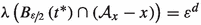and we can compute the double integral

  $$\begin{aligned} \int _{I_0}\int _{B_{\nicefrac {\varepsilon }{2}}\left( t^{*}\right) }\chi _{{\mathcal {A}}_x-x}\left( t\right) ~\textrm{d}t\,\textrm{d}x=\int _{I_0}\varepsilon ^d~\textrm{d}x=\frac{\varepsilon ^{2d}}{2^d}. \end{aligned}$$

  Fubini’s theorem implies that exists for almost every $t\in B_{\nicefrac {\varepsilon }{2}}\left( t^{*}\right)$ and we may change the order of integration to obtain

  

  This implies (i.e., that $M_t$ is of full measure in $I_0$) for almost every $t\in B_{\nicefrac {\varepsilon }{2}}\left( t^{*}\right)$.

• (b) Since holds by Lemma 5.2.3a), part a) of the current lemma implies the existence of $t_0\in {\mathcal {A}}_0\cap C_m^{\prime }\cap B_{\nicefrac {\varepsilon }{2}}\left( t^{*}\right)$ such that $M_{t_0}$ is of full measure in $I_0$. From Lemma 5.2.3b), we additionally obtain $M_{t_0}+t_0\subseteq B_{\nicefrac {3\varepsilon }{4}}\left( z^{*}\right)$, which implies

  

  Lemma 5.2.3a) allows us to compute

  

$\square$

Now, we propagate the phase from $t_0$ onto $M_{t_0}+t_0$ to obtain the following theorem.

Theorem 5.2.5

There exist $\gamma _m\in {\mathbb {T}}$ and a measurable subset ${\mathcal {B}}_0\subseteq {{\mathbb {R}}}^d$ satisfying as well as ${\tilde{f}}(z)=\gamma _m\cdot f(z)$ for every $z\in {\mathcal {B}}_0$.

Proof

As indicated before, we choose ${\mathcal {B}}_0:=M_{t_0}+t_0$ with $t_0$ from Lemma 5.2.4b). Consequently, it holds . Since $t_0\in {\mathcal {A}}_0\cap C_m^{\prime }$, i.e., $\left| f(t_0)\right| =\left| {\tilde{f}}(t_0)\right| \ne 0$, we may define

$$\begin{aligned} \gamma _m:=\frac{{\tilde{f}}(t_0)}{f(t_0)}\in {\mathbb {T}}. \end{aligned}$$

Now, for every $z\in {\mathcal {B}}_0$, it holds $x:=z-t_0\in M_{t_0}$, i.e., $x\in I_0\subseteq D_g$ and $z=t_0+x\in {\mathcal {A}}_x$. This implies

$$\begin{aligned} {\tilde{f}}(z)=f(z)\cdot \frac{\overline{f(t_0)}}{\overline{{\tilde{f}}(t_0)}}=\gamma _m f(z). \end{aligned}$$

$\square$

5.3 Phase Propagation

Starting from Theorem 5.2.5, we will now propagate the phase $\gamma$ onto almost all of $C_m^{\prime }$. Recall that we assumed w.l.o.g. that $C(f)=C(f)^{*}$. This allows us to prove the following lemma.

Lemma 5.3.1

The following statements hold true.

• (a) It holds $C_m^{*}\subseteq C_m$.

• (b) It holds $(C_m^{\prime })^{*}=C_m^{\prime }$.

Proof

• (a) Let $z\in C_m^{*}$. In particular, z is an accumulation point of $\text {supp}(f)$, which implies $z\in \text {supp}(f)$ since $\text {supp}(f)$ is closed. Additionally, $B_L(z)$ contains an element of $C_m$ and because of $B_L(0)\subseteq D_g$, this implies $z\in C_m$.

• (b) The inclusion $(C_m^{\prime })^{*}\subseteq C_m^{\prime }$ follows immediately from a) and $C(f)=C(f)^{*}$.

  Conversely, when $z\in C_m^{\prime }$, we combine $B_L(0)\subseteq D_g$ and $C(f)\subseteq \text {supp}(f)$ to obtain for all $0<\varepsilon <L$. Using $C(f)=C(f)^{*}$, we obtain $z\in (C_m^{\prime })^{*}$.

$\square$

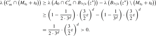
We will propagate the phase iteratively along the sets $\left( {\mathcal {P}}_k\right) _{k\in {\mathbb {N}}_0}$, defined by

$$\begin{aligned} {\mathcal {P}}_0:=\left( {\mathcal {B}}_0\cap C_m^{\prime }\right) ^{*} \end{aligned}$$

as well as

$$\begin{aligned} {\mathcal {P}}_{k+1}:=\left( {\mathcal {P}}_k+D_g\right) \cap C_m^{\prime }\quad \quad (k\in {\mathbb {N}}_0). \end{aligned}$$

The most important properties of these sets are summarized in the following lemma.

Lemma 5.3.2

The following statements hold true.

• (a) It holds $\emptyset \ne {\mathcal {P}}_0\subseteq C_m^{\prime }$.

• (b) For every $k\in {\mathbb {N}}_0$, it holds ${\mathcal {P}}_k\subseteq {\mathcal {P}}_k^{*}$.

• (c) It holds $C_m^{\prime }=\bigcup _{k\in {\mathbb {N}}_0} {\mathcal {P}}_k$.

Proof

• (a) ${\mathcal {P}}_0\ne \emptyset$ follows from Theorem 5.2.5 and Lebesgue’s density theorem. ${\mathcal {P}}_0\subseteq C_m^{\prime }$ follows from Lemma 5.3.1b).

• (b) We prove this statement by induction. Just as above, ${\mathcal {P}}_0^{*}={\mathcal {P}}_0$ follows from Lebesgue’s density theorem. Now, assume that ${\mathcal {P}}_k\subseteq {\mathcal {P}}_k^{*}$ holds true for some $k\in {\mathbb {N}}_0$ and pick $z\in {\mathcal {P}}_{k+1}$. By Lemma 5.3.1b), z is a density point of $C_m^{\prime }$. Furthermore, there exists $x\in D_g$ satisfying $z-x\in {\mathcal {P}}_k\subseteq {\mathcal {P}}_k^{*}$ by the induction hypothesis. Since the Lebesgue measure is translation-invariant, it follows that z is a density point of ${\mathcal {P}}_k+x$ and thus of ${\mathcal {P}}_k+D_g$. Now, it is easy to show that z is also a density point of $({\mathcal {P}}_k+D_g)\cap C_m^{\prime }={\mathcal {P}}_{k+1}$.

• (c) The inclusion “$\supseteq$” is clear since ${\mathcal {P}}_k\subseteq C_m^{\prime }$ holds by definition when $k\in {\mathbb {N}}$ and by part a) when $k=0$. For the proof of the converse inclusion, fix $z\in {\mathcal {P}}_0$ which exists by part a) and also implies $z\in C_m^{\prime }$. Now, let $z^{\prime }\in C_m^{\prime }$ be arbitrary. By Lemma 5.2.1, there exist $y_0,\dots ,y_n\in C_m^{\prime }$ satisfying $y_0=z$, $y_n=z^{\prime }$ and $x_j:=y_j-y_{j-1}\in D_g$ for every $1\le j\le n$. Inductively, this implies $z^{\prime }\in {\mathcal {P}}_n\subseteq \bigcup _{k\in {\mathbb {N}}_0} {\mathcal {P}}_k$.

$\square$

Recall that Theorem 5.2.5 states the existence of $\gamma _m\in {\mathbb {T}}$ satisfying ${\tilde{f}}(z)=\gamma _m\cdot f(z)$ for all $z\in {\mathcal {B}}_0$, which is clearly a set of full measure in ${\mathcal {P}}_0$. As mentioned before, our goal is now to propagate the phase in each step from (most of) ${\mathcal {P}}_k$ to (most of) ${\mathcal {P}}_{k+1}$. First, we prove a local version of this iteration.

Lemma 5.3.3

Let $k\in {\mathbb {N}}_0$ and assume that there exists a subset ${\mathcal {E}}_k\subseteq {\mathcal {P}}_k$ of full measure satisfying ${\tilde{f}}(t)=\gamma _m\cdot f(t)$ for every $t\in {\mathcal {E}}_k$. Then, for every $z\in {\mathcal {P}}_{k+1}$, there exists an open neighborhood $U_z$ of z such that ${\tilde{f}}\left( z^{\prime }\right) =\gamma _m\cdot f\left( z^{\prime }\right)$ holds for almost every $z^{\prime }\in U_z$.

Proof

Let $z\in {\mathcal {P}}_{k+1}$. By definition, there exists $y\in {\mathcal {P}}_k$ satisfying $x:=z-y\in D_g$ and since $D_g$ is open, we can choose $\varepsilon >0$ satisfying $B_{\varepsilon }(x)\subseteq D_g$. Now, pick $0<\alpha <1$. We will show

By Lemma 5.3.2, it holds $y\in {\mathcal {P}}_{k}^{*}$. Hence, we may choose $\delta >0$ satisfying

and assume w.l.o.g. that $n:=\frac{\varepsilon }{\delta }-\frac{1}{2}\in {\mathbb {N}}$. For all $j\in {\mathbb {Z}}^d$ satisfying $\Vert j\Vert =\Vert j\Vert _{\infty }\le n$, this implies $\Vert \delta j\Vert \le \varepsilon -\frac{\delta }{2}<\varepsilon$ and therefore $x+\delta j\in B_{\varepsilon }(x)\subseteq D_g$. Additionally, we obtain

$$\begin{aligned} \bigcup \limits _{\Vert j\Vert \le n} B_{\nicefrac {\delta }{2}}(y)+(x+\delta j)\subseteq B_{\varepsilon }(z)=:U_z, \end{aligned}$$

where the union on the left-hand side is disjoint. As a consequence,

$$\begin{aligned} M:=\bigcup \limits _{\Vert j\Vert \le n}\left( \left( {\mathcal {E}}_k\cap B_{\nicefrac {\delta }{2}}(y)\right) +(x+\delta j)\right) \cap {\mathcal {A}}_{x+\delta j} \end{aligned}$$

is also a subset of $U_z$ and since this union is still disjoint, we may compute

Finally, we pick $z^{\prime }\in M$. By definition, there exists $j\in {\mathbb {Z}}^d$ satisfying $\Vert j\Vert \le n$ and $t\in {\mathcal {E}}_k$ such that $z^{\prime }\in {\mathcal {A}}_{x+\delta j}$ as well as $z^{\prime }=t+(x+\delta j)$, which implies $f\left( z^{\prime }\right) \overline{f(t)}={\tilde{f}}\left( z^{\prime }\right) \overline{{\tilde{f}}(t)}$. Since $t\in {\mathcal {E}}_k\subseteq {\mathcal {P}}_k\subseteq C_m^{\prime }\subseteq C(f)$, this implies ${\tilde{f}}\left( z^{\prime }\right) =\gamma _m\cdot f\left( z^{\prime }\right)$ and we are able to conclude that

As $0<\alpha <1$ was picked arbitrarily, it follows ${\tilde{f}}\left( z^{\prime }\right) =\gamma _m\cdot f\left( z^{\prime }\right)$ for almost every $z^{\prime }\in U_z$. $\square$

We can now use the inner regularity of the Lebesgue measure to obtain global phase propagation.

Lemma 5.3.4

Let $k\in {\mathbb {N}}_0$ and assume that there exists a subset ${\mathcal {E}}_k\subseteq {\mathcal {P}}_k$ of full measure satisfying ${\tilde{f}}(t)=\gamma _m\cdot f(t)$ for every $t\in {\mathcal {E}}_k$. Then, there exists a subset ${\mathcal {E}}_{k+1}\subseteq {\mathcal {P}}_{k+1}$ of full measure satisfying ${\tilde{f}}(t)=\gamma _m\cdot f(t)$ for every $t\in {\mathcal {E}}_{k+1}$.

Proof

By Lemma 5.3.3, for every $z\in {\mathcal {P}}_{k+1}$, there exists an open neighborhood $U_z$ of z as well as a subset ${\mathcal {E}}_z\subseteq U_z$ of full measure satisfying ${\tilde{f}}\left( z^{\prime }\right) =\gamma _m\cdot f\left( z^{\prime }\right)$ for every $z^{\prime }\in {\mathcal {E}}_z$. Since ${\mathcal {P}}_{k+1}$ is measurable (by induction), there exists a sequence $\left( K_n\right) _{n\in {\mathbb {N}}}$ of compact subsets of ${\mathcal {P}}_{k+1}$ such that $\bigcup _{n\in {\mathbb {N}}} K_n$ is of full measure in ${\mathcal {P}}_{k+1}$. For fixed $n\in {\mathbb {N}}$, the fact that $K_n\subseteq \bigcup _{z\in K_n} U_z$ together with the compactness of $K_n$ implies the existence of a finite set $J_n\subseteq K_n$ satisfying $K_n\subseteq \bigcup _{z\in J_n} U_z$. Now, the set

$$\begin{aligned} {\mathcal {E}}^{(n)}:=\bigcup \limits _{z\in J_n}{\mathcal {E}}_z, \end{aligned}$$

is clearly of full measure in $K_n$ and we obtain ${\tilde{f}}\left( z^{\prime }\right) =\gamma _m\cdot f\left( z^{\prime }\right)$ for every $z^{\prime }\in {\mathcal {E}}^{(n)}$ Finally, we define

$$\begin{aligned} {\mathcal {E}}_{k+1}:=\left( \bigcup \limits _{n\in {\mathbb {N}}}{\mathcal {E}}^{(n)}\right) \cap {\mathcal {P}}_{k+1}. \end{aligned}$$

Then clearly, ${\mathcal {E}}_{k+1}$ is of full measure in ${\mathcal {P}}_{k+1}$ and satisfies ${\tilde{f}}\left( z^{\prime }\right) =\gamma _m\cdot f\left( z^{\prime }\right)$ for every $z^{\prime }\in {\mathcal {E}}_{k+1}$, which proves the claim. $\square$

We are now able to complete the proof of Theorem 5.1.8: Recall that the hypothesis of Lemma 5.3.4 is satisfied for $k=0$ by Theorem 5.2.5. For every $k\in {\mathbb {N}}$, Lemma 5.3.4 inductively implies the existence of a subset ${\mathcal {E}}_k\subseteq {\mathcal {P}}_k$ of full measure satisfying ${\tilde{f}}(t)=\gamma _m\cdot f(t)$ for every $t\in {\mathcal {E}}_k$. Now,

$$\begin{aligned} {\mathcal {E}}:=\bigcup \limits _{k\in {\mathbb {N}}_0}{\mathcal {E}}_k. \end{aligned}$$

is a set of full measure in $\bigcup _{k\in {\mathbb {N}}_0}{\mathcal {P}}_k=C_m^{\prime }$ (by Lemma 5.3.2) and satisfies ${\tilde{f}}(z)=\gamma _m\cdot f(z)$ for every $z\in {\mathcal {E}}$. Finally, for $z\in C_m{\setminus } C_m^{\prime }$, we have ${\tilde{f}}(z)=0=\gamma _m\cdot f(z)$.

5.4 Examples

We conclude this section by applying Theorem 5.1.8 to a few interesting windows. First however, we make a general remark towards understanding the result.

Remark 5.4.1

Even though Theorem 5.1.8 is easy to understand from an abstract point of view, it can sometimes be hard to decide whether a given signal is g-connected. Consider e.g., a closed, symmetric set $A\subseteq {{\mathbb {R}}}^d$ of positive measure satisfying $0\notin A$. For $X:={{\mathbb {R}}}^d\setminus A$, we may ask the following question: Does there exist $f\in L^2({{\mathbb {R}}}^d)$ which is not connected with respect to translations in X? If the answer is always “yes”, this would imply that for the considered window classes, phase retrieval is equivalent to $\Omega _g$ being of full measure in ${{\mathbb {R}}}^{2d}$. Otherwise, any set X for which the answer is “no” could give us a clue towards constructing a window that does phase retrieval despite $\Omega _g$ not being of full measure in ${{\mathbb {R}}}^{2d}$. However, we are currently unable to answer this question.

Theorem 5.1.8 immediately yields phase retrieval for every window $g\in L^{2,\exp }({{\mathbb {R}}}^d)$ or $g\in L^{2,+}({{\mathbb {R}}})$ that vanishes nowhere on $(0,\infty )$. This allows us to revisit some important windows for phase retrieval.

Examples 5.4.2

For $a>0$, let $\gamma _a,\varphi _a,\psi _a\in L^2({{\mathbb {R}}})$ be defined by $\gamma _a(t):=e^{-a\pi t^2}$, $\varphi _a(t):=e^{-a|t|}$ and $\psi _a(t):=\frac{1}{a+2\pi it}$ for (almost) all $t\in {{\mathbb {R}}}$. Additionally, let ${\tilde{\varphi }}_a:=\varphi _a\cdot \chi _{(0,\infty )}$ as well as ${\tilde{\psi }}_a:=\psi \cdot \chi _{(0,\infty )}$. Then, $\gamma _a,\varphi _a,\psi _a,{\tilde{\varphi }}_a$ and ${\tilde{\psi }}_a$ do phase retrieval.

The fact that the Gaussian window $\gamma _a$ does phase retrieval is well-known [16]. Phase retrieval for $\varphi _a$ and ${\tilde{\varphi }}_a$ can be obtained through explicit calculation of their ambiguity functions [14]. Theorem 5.1.8 also yields phase retrieval for each of the three windows but requires no explicit calculation of the ambiguity function.

Phase retrieval for the window $\psi _a$ also follows from the observations in [14] and can not be obtained by applying Theorem 5.1.8. However, Theorem 5.1.8 implies phase retrieval for ${\tilde{\psi }}_a$, which appears to be a new result.

Finally, we consider some compactly supported windows. These are obviously inadequate for global phase retrieval but can still be used for phase retrieval on special signal classes.

Example 5.4.3

Let $g_{a,b}:=\chi _{[a,b]}$ for some $a,b\in {{\mathbb {R}}}$ satisfying $a<b$. Then, a signal $f\in L^2({{\mathbb {R}}}^d)$ is phase retrievable with respect to $g_{a,b}$ if and only if f has no hole of length $b-a$, i.e., if the implication

$$\begin{aligned} f\vert _{(t,t+b-a)}\equiv 0 ~\text {a.e.}\quad \quad \Rightarrow \quad \quad f\vert _{(-\infty ,t)}\equiv 0~\text {a.e.}\quad \text {or}\quad f\vert _{(t+b-a,\infty )}\equiv 0~\text {a.e.} \end{aligned}$$

holds true for every $t\in {{\mathbb {R}}}$.

This follows from Theorem 5.1.8 as it is easy to show that $D_{g_{a,b}}=(-(b-a),b-a)$ and that a signal f is g-connected if and only if it has no holes of length $b-a$. As in the discrete setting, we obtain the intuition that g has to be “long enough” to bridge over possible holes of f. It is possible to “thin out” the support of g even further.

Example 5.4.4

Let $g_{a_1,a_2,b_1,b_2}:=\chi _{[a_1,a_2]}+\chi _{[b_1,b_2]}$ for some $a_1,a_2,b_1,b_2\in {{\mathbb {R}}}$ satisfying$a_1<a_2<b_1<b_2$ as well as $b_1-a_2<\max \{a_2-a_1,b_2-b_1\}$. Then, a signal $f\in L^2({{\mathbb {R}}}^d)$ is phase retrievable with respect to $g_{a_1,a_2,b_1,b_2}$ if and only if f has no hole of length $b_2-a_1$ in the sense of Example 5.4.3.

In this case, we have $D_{g_{a_1,a_2,b_1,b_2}}=(-(b_2-a_1),b_2-a_1)$, which follows from the upper bound on $b_1-a_2$. A variation of this example also shows that things can get out of control very easily: When considering $g_{a_1,a_2,b_1,b_2}$ for the case $b_1-a_2>\max \{a_2-a_1,b_2-b_1\}$, we obtain

$$\begin{aligned} D_{g_{a_1,a_2,b_1,b_2}}=(-(b_2-a_1),-(b_1-a_2))\cup (-m,m)\cup (b_1-a_2,b_2-a_1) \end{aligned}$$

where $m:=\max \{a_2-a_1,b_2-b_1\}$. Classifying all g-connected signals appears to be a difficult task in this case. (Note that we can say at least that “no hole of length m” is a sufficient condition and “no hole of length $b_2-a_1$” is a necessary condition for g-connectedness.)

6 Concluding Remarks

The goal of this paper was to provide useful criteria for STFT phase retrieval on ${\mathbb {Z}}$, ${\mathbb {Z}}_d$ and ${{\mathbb {R}}}^d$. In summary, we proved a full characterization of phase retrieval for the following combinations of windows and signals:

• (1) $g\in \ell ^2({\mathbb {Z}})$ of exponential decay or one-sided, $f\in \ell ^2({\mathbb {Z}})$ arbitrary

• (2) $g\in {{\mathbb {C}}}^d_L$, $f\in {{\mathbb {C}}}^d$ L-separated

• (3) $g\in L^2({{\mathbb {R}}}^d)$ of exponential decay or one-dimensional and one-sided, $f\in L^2({{\mathbb {R}}}^d)$ arbitrary

This corresponds to identifying both the possibilities and the limitations of phase retrieval for a single given window (i.e., a given measurement method), which appears to be highly useful in applications.

Large similarities between the different settings are evident (especially when comparing $G={\mathbb {Z}}$ and $G={{\mathbb {R}}}^d$) with the common theme within all the different scenarios being the fact that the characterizations only depend on the supports of window and signal. This leads to conditions that are usually easy to understand and to check (at least in the discrete settings) and showcase the fact that disconnectedness (in one way or another) is (up to only a few pathological counterexamples in the cyclic case) essentially the only obstacle for STFT phase retrieval.

References

Akutowicz, E.J.: On the determination of the phase of a Fourier integral. I. Trans. Am. Math. Soc. 83(1), 179–192 (1956). https://doi.org/10.2307/1992910
Akutowicz, E.J.: On the determination of the phase of a Fourier integral. II. Proc. Am. Math. Soc. 8(2), 234–238 (1957). https://doi.org/10.2307/2033718
Alaifari, R., Daubechies, I., Grohs, P., Thakur, G.: Reconstructing real-valued functions from unsigned coefficients with respect to wavelet and other frames. J. Fourier Anal. Appl. 23(6), 1480–1494 (2017). https://doi.org/10.1007/s00041-016-9513-7
Alaifari, R., Daubechies, I., Grohs, P., Yin, R.: Stable phase retrieval in infinite dimensions. Found. Comput. Math. 19(4), 869–900 (2019). https://doi.org/10.1007/s10208-018-9399-7
Alaifari, R., Wellershoff, M.: Stability estimates for phase retrieval from discrete Gabor measurements. J. Fourier Anal. Appl. 27(2), 1–31 (2021). https://doi.org/10.1007/s00041-020-09802-1
Alaifari, R., Wellershoff, M.: Uniqueness of STFT phase retrieval for bandlimited functions. Appl. Comput. Harmon. Anal. 50, 34–48 (2021). https://doi.org/10.1016/j.acha.2020.08.003
Balan, R., Casazza, P., Edidin, D.: On signal reconstruction without phase. Appl. Comput. Harmon. Anal. 20(3), 345–356 (2006). https://doi.org/10.1016/j.acha.2005.07.001
Bojarovska, I., Flinth, A.: Phase retrieval from Gabor measurements. J. Fourier Anal. Appl. 22(3), 542–567 (2016). https://doi.org/10.1007/s00041-015-9431-0
Conca, A., Edidin, D., Hering, M., Vinzant, C.: An algebraic characterization of injectivity in phase retrieval. Appl. Comp. Harmon. Anal. 38(2), 346–356 (2015). https://doi.org/10.1016/j.acha.2014.06.005
da Silva, J.C., Menzel, A.: Elementary signals in ptychography. Opt. Express 23(26), 33812–33821 (2015). https://doi.org/10.1364/oe.23.033812
Eldar, Y.C., Sidorenko, P., Mixon, D.G., Barel, S., Cohen, O.: Sparse phase retrieval from short-time Fourier measurements. IEEE Signal Process. Lett. 22(5), 638–642 (2015). https://doi.org/10.1109/lsp.2014.2364225
Griffin, D., Lim, J.: Signal estimation from modified short-time Fourier transform. IEEE Trans. Acoust. Speech Signal Process. 32(2), 236–243 (1984). https://doi.org/10.1109/tassp.1984.1164317
Gröchenig, K.: Foundations of Time-Frequency Analysis. Birkhäuser Boston Inc., Boston (2001)
Gröchenig, K., Jaming, P., Malinnikova, E.: Zeros of the Wigner distribution and the short-time Fourier transform. Rev. Mat. Complut. 33(3), 723–744 (2020). https://doi.org/10.1007/s13163-019-00335-w
Grohs, P., Koppensteiner, S., Rathmair, M.: Phase retrieval: uniqueness and stability. SIAM Rev. 62(2), 301–350 (2020). https://doi.org/10.1137/19m1256865
Grohs, P., Rathmair, M.: Stable Gabor phase retrieval and spectral clustering. Commun. Pure Appl. Math. 72(5), 981–1043 (2019). https://doi.org/10.1002/cpa.21799
Jaganathan, K., Eldar, Y.C., Hassibi, B.: STFT phase retrieval: uniqueness guarantees and recovery algorithms. IEEE J. Sel. Top. Signal Process. 10(4), 770–781 (2016). https://doi.org/10.1109/jstsp.2016.2549507
Jaming, P.: Phase retrieval techniques for radar ambiguity problems. J. Fourier Anal. Appl. 5(4), 309–329 (1999). https://doi.org/10.1007/bf01259373
Jaming, P., Kellay, K., Perez, R.: Phase retrieval for wide band signals. J. Fourier Anal. Appl. 26(4), 54 (2020). https://doi.org/10.1007/s00041-020-09767-1
Katznelson, Y.: An Introduction to Harmonic Analysis. Cambridge University Press, Cambridge (2004)
Li, L., Cheng, C., Han, D., Sun, Q., Shi, G.: Phase retrieval from multiple-window short-time Fourier measurements. IEEE Signal Process. Lett. 24(4), 372–376 (2017). https://doi.org/10.1109/lsp.2017.2663668
Mallat, S., Waldspurger, I.: Phase retrieval for the Cauchy wavelet transform. J. Fourier Anal. Appl. 21(6), 1251–1309 (2015). https://doi.org/10.1007/s00041-015-9403-4
Nawab, S., Quatieri, T., Lim, J.: Signal reconstruction from short-time Fourier transform magnitude. IEEE Trans. Acoust. Speech Signal Process. 31(4), 986–998 (1983). https://doi.org/10.1109/tassp.1983.1164162
Preskitt, B., Saab, R.: Admissible measurements and robust algorithms for ptychography. J. Fourier Anal. Appl. 27(2), 1–39 (2021). https://doi.org/10.1007/s00041-021-09811-8
Rudin, W.: Real and Complex Analysis, 3rd edn. McGraw-Hill, New York (1987)
Rudin, W.: Fourier Analysis on Groups. Wiley-Interscience, New York (1962)
Simon, B.: Harmonic Analysis. American Mathematical Society, Providence (2015)
Stein, E.M., Shakarchi, R.: Complex Analysis. Princeton Lectures in Analysis. Princeton University Press, Princeton (2003)
Acknowledgements
The author would like to thank Hartmut Führ for fruitful discussions on the topic as well as careful reading of the manuscript. Moreover, the author highly appreciates the useful critique of the anonymous referees, which considerably helped to improve this article.
Funding
Open Access funding enabled and organized by Projekt DEAL.
Author information
Authors and Affiliations
Corresponding author
Additional information
Communicated by Philippe Jaming.
Publisher's Note
Springer Nature remains neutral with regard to jurisdictional claims in published maps and institutional affiliations.
Rights and permissions
Open Access This article is licensed under a Creative Commons Attribution 4.0 International License, which permits use, sharing, adaptation, distribution and reproduction in any medium or format, as long as you give appropriate credit to the original author(s) and the source, provide a link to the Creative Commons licence, and indicate if changes were made. The images or other third party material in this article are included in the article’s Creative Commons licence, unless indicated otherwise in a credit line to the material. If material is not included in the article’s Creative Commons licence and your intended use is not permitted by statutory regulation or exceeds the permitted use, you will need to obtain permission directly from the copyright holder. To view a copy of this licence, visit http://creativecommons.org/licenses/by/4.0/.
About this article
Cite this article
Bartusel, D. Injectivity Conditions for STFT Phase Retrieval on \({\mathbb {Z}}\), \({\mathbb {Z}}_d\) and \({{\mathbb {R}}}^d\). J Fourier Anal Appl 29, 53 (2023). https://doi.org/10.1007/s00041-023-10026-2
Received:
Revised:
Accepted:
Published:
DOI: https://doi.org/10.1007/s00041-023-10026-2