Coalescence of Geodesics and the BKS Midpoint Problem in Planar First-Passage Percolation

Abstract

We consider first-passage percolation on $\mathbb{Z}^{2}$ with independent and identically distributed weights whose common distribution is absolutely continuous with a finite exponential moment. Under the assumption that the limit shape has more than 32 extreme points, we prove that geodesics with nearby starting and ending points have significant overlap, coalescing on all but small portions near their endpoints. The statement is quantified, with power-law dependence of the involved quantities on the length of the geodesics.

The result leads to a quantitative resolution of the Benjamini–Kalai–Schramm midpoint problem. It is shown that the probability that the geodesic between two given points passes through a given edge is smaller than a power of the distance between the points and the edge.

We further prove that the limit shape assumption is satisfied for a specific family of distributions.

Lastly, related to the 1965 Hammersley–Welsh highways and byways problem, we prove that the expected fraction of the square {−n,…,n}² which is covered by infinite geodesics starting at the origin is at most an inverse power of n. This result is obtained without explicit limit shape assumptions.

1 Introduction

First-passage percolation is a model for a random metric space, formed by a random perturbation of an underlying base space. Since its introduction by Hammersley–Welsh in 1965 [HW65], it has been studied extensively in the probability and statistical physics literature. We refer to [Kes86] for general background and to [ADH17] for more recent results.

We study first-passage percolation on the square lattice $(\mathbb{Z}^{2},E(\mathbb{Z}^{2}))$ with independent and identically distributed (IID) random environment. The model is specified by a weight distribution G, a probability measure on the non-negative reals. Each edge $e\in E(\mathbb{Z}^{2})$ is assigned a random passage time t_e with distribution G, independently between edges. Then, each finite path p in $\mathbb{Z} ^{2}$ is assigned the passage time

$$ T(p):=\sum _{e\in p} t_{e}. $$

(1.1)

A random metric T on $\mathbb{Z}^{2}$ is defined by setting the passage time between $u,v\in \mathbb{Z} ^{2}$ to

$$ T(u,v):=\inf _{p} T(p), $$

where the infimum ranges over all paths connecting u and v. Any path achieving the infimum is termed a geodesic between u and v. A unique geodesic exists when G is atomless (in particular, under our assumption (ABS) below) and will be denoted γ(u,v) (and regarded as a subgraph of $\mathbb{Z}^{2}$). The focus of first-passage percolation is the study of the large-scale properties of the random metric T and its geodesics.

1.1 Results

We proceed to describe our main results. Background and further discussion is provided in Sect. 1.4.

Throughout we assume that G possesses an exponential moment,

$$ \exists \alpha >0 \ \text{ so that } \ \mathbb{E} \big[ \exp (\alpha t_{e}) \big]< \infty $$

(EXP)

and also that

$$ G\text{ is absolutely continuous}. $$

(ABS)

The first-order behavior of the metric T is governed by the following result. Define the metric ball of radius t by

$$ B(t):=\big\{ \,v\in \mathbb{Z}^{2}:\, T(0,v)\leq t\,\big\} + \left [- \frac{1}{2},\frac{1}{2}\right ] ^{2}. $$

Limit Shape Theorem 1

Cox and Durrett [TD81]

For any distribution G satisfying (EXP) and (ABS), there exists a deterministic convex set $\mathcal {B}_{G}$ such that for all ϵ>0,

$$ \mathbb{P} \Big( \exists t_{0}>0 \textit{ such that }\ \forall t\geq t_{0}, \quad (1-\epsilon )\mathcal {B}_{G} \subseteq \frac{B(t)}{t}\subseteq (1+ \epsilon )\mathcal {B}_{G} \Big) =1. $$

The set $\mathcal {B} _{G}$ is called the limit shape corresponding to G. The theorem holds under weaker assumptions but the above generality suffices for the purposes here.

1.1.1 Coalescence of geodesics

Our first result concerns the coalescence of geodesics with nearby starting and ending points. It is shown that, with high probability, such geodesics overlap almost entirely, differing only in short segments near their endpoints. The statement is quantified, obtaining power-law dependence of the involved quantities on the length of the geodesics.

We define $\operatorname{Sides}(\mathcal {B}_{G})$ as the number of sides of $\mathcal {B}_{G}$: if $\mathcal {B}_{G}$ is a polygon then $\operatorname{Sides}(\mathcal {B}_{G})$ is its number of edges while if $\mathcal {B}_{G}$ is not a polygon then $\operatorname{Sides}(\mathcal {B}_{G}):=+\infty$ (equivalently, $\operatorname{Sides}(\mathcal {B}_{G})$ is the number of extreme points of $\mathcal {B}_{G}$). Our proof requires a lower bound on $\operatorname{Sides}(\mathcal {B}_{G})$. This assumption is weaker than the condition that the limit shape be strictly convex, a condition which is believed, but not proved, to follow from assumption (ABS) (see [ADH17, Question 11]). Theorem 1.5 below identifies an explicit class of distributions G satisfying (EXP), (ABS) and the required lower bound on $\operatorname{Sides}(\mathcal {B}_{G})$ so that our result holds unconditionally for this class.

We write ∥⋅∥ for the ℓ₁ norm on $\mathbb{R}^{2}$. For n≥0, set

$$ \Lambda _{n}:=[-n,n]^{2}\cap \mathbb{Z}^{2}. $$

Theorem 1.1

Suppose G satisfies (EXP), (ABS) and $\operatorname{Sides}(\mathcal {B}_{G})>32$. There exists C>0 (depending only on G) such that for each 0<ϵ≤1/17, each δ≥0 and all $y\in \mathbb{Z}^{2}$ with ∥y∥≥2,

$$\begin{aligned} &\mathbb{P} \Big(\exists u,z\in \Lambda _{\|y\|^{1/8 -\epsilon}}\, \exists v,w\in (y+\Lambda _{\|y\|^{1/8 -\epsilon}})\quad \!\! \big| \gamma (u,v) \triangle \gamma (z,w) \big| > \|y\|^{1-\delta } \Big) \\ &\quad\le \! \frac{C\log ^{2} \|y\|}{\|y\|^{\epsilon -\delta /8 }}, \end{aligned}$$

where p₁△p₂ is the set of edges belonging to exactly one of the paths p₁,p₂.

The theorem thus shows that all geodesics which start at distance at most ∥y∥^1/8−ϵ from the origin and end at distance at most ∥y∥^1/8−ϵ from y coalesce with high probability. In this sense, it is shown that the coalescence exponent of first-passage percolation is at least 1/8. This is the first result establishing the positivity of the coalescence exponent for an explicit class of weight distributions in first-passage percolation (using Theorem 1.5); see Sect. 1.4.1 for further discussion.

We point out that the coalescence set of two geodesics is necessarily a path. This follows from the fact that there is a unique geodesic between every pair of points. See Fig. 1 for simulation results showing the phenomenon of coalescence.

Figure 1

A computer simulation of the geodesics from (−1000,0) to (1000,0) (blue and purple) and from (−1000,30) to (1000,30) (red and purple) in first-passage percolation on $\mathbb{Z} ^{2}$ with weight distribution uniform on [0,1]. The pictures depict the geodesics in independent samples of the environment. Theorem 1.1 states that nearby geodesics coalesce with high probability. The geodesics in the fourth simulation did not coalesce and, moreover, were far from each other for most of the way. This is compatible with our results as Proposition 1.7 shows that geodesics which stay close to each other for a significant amount of time have a very high probability to coalesce. Color figure online.

1.1.2 The influence of edges

The passage time of the geodesic between given endpoints is naturally a function of the weights assigned to all edges. To what extent is this passage time influenced by the weight assigned to a specific edge? This notion is formalized here by the probability that the geodesic passes through that edge. It is clear that the influence of edges near the endpoints cannot be uniformly small, but it is not clear whether the influence must diminish for edges far from the endpoints. This issue was highlighted by Benjamini–Kalai–Schramm [BKS03] in their seminal study of the variance of the passage time, where the following problem, later termed the BKS midpoint problem, was posed: Consider the geodesic between 0 and v. Does the probability that it passes at distance 1 from v/2 tend to zero as ∥v∥→∞? A proof that this probability tends to zero as a power of ∥v∥ (and analogous estimates for other edges) would simplify the argument of [BKS03].

The BKS midpoint problem on the square lattice was resolved positively by Damron–Hanson [DH17] under the assumption that the limit shape boundary is differentiable and then resolved unconditionally by Ahlberg–Hoffman [AH19]. While both resolutions apply to the more general setup of ergodic edge weights (rather than simply IID), they also share the drawback that no quantitative decay rate for the probability is obtained. As a consequence of our quantitative control on the coalescence of geodesics, we are able to prove power-law decay rates for the influence of edges. These apply, in particular, for the “midpoint edges”, yielding a quantitative resolution of the BKS midpoint problem.

Theorem 1.2

Suppose G satisfies (EXP), (ABS) and $\operatorname{Sides}(\mathcal {B}_{G})>40$. There exists C>0 (depending only on G) such that for all $u,v,z\in \mathbb{Z}^{2}$,

$$ \mathbb{P}\big(z\in \gamma (u,v)\big)\le \frac{C\log ^{2} (D_{z}^{u,v}+2)}{(D_{z}^{u,v})^{1/16}}, $$

(1.2)

where $D_{z}^{u,v}:=\min \{\|u-z\|,\|v-z\|\}$.

A variant of the result may also be obtained under the weaker assumption $\operatorname{Sides}(\mathcal {B}_{G})>32$, see (3.12).

It is clear that one cannot have a decay rate in (1.2) which is uniform in z at a given distance from u and v and is faster than a power law, since for any integer $0< k\le \frac{1}{2}\|u-v\|$ the geodesic γ(u,v) must pass through at least one vertex z with $D_{z}^{u,v}=k$.

Theorem 1.2 implies, as a special case, that the probability that the origin lies on the geodesic between (−n,0) and (n,0) is smaller than a power of n. In fact, the method used to derive Theorem 1.2 allows to prove a stronger fact: the probability that there exists an integer s for which the origin lies on a geodesic from (−n,s) to (n,s) is smaller than a power of n. We state this fact in our next theorem.

Theorem 1.3

Suppose G satisfies (EXP), (ABS) and $\operatorname{Sides}(\mathcal {B}_{G})>40$. There exists C>0 (depending only on G) such that for all integer n≥2,

$$ \mathbb{P}\Big( (0,0)\in \bigcup _{s\in \mathbb{Z}}\gamma \big( (-n,s),(n,s) \big) \Big) \le \frac{C\log ^{2}n}{n^{1/24}}. $$

Our methods also allow to prove related statements in which the horizontal geodesics are replaced by geodesics with a fixed slope.

We point out that the theorem is related to the well-known problem of proving that there are no infinite bigeodesics (doubly-infinite paths for which every finite sub-path is a geodesic) in first-passage percolation. Indeed, the latter problem can be rephrased as proving that the probability that there exist two points at distance n from the origin such that the geodesic between the points passes through the origin, tends to zero with n.

1.1.3 Highways and byways

In their seminal paper [HW65], Hammersley and Welsh coined the notions of highways and byways. An edge of $\mathbb{Z}^{2}$ is called a highway edge if it belongs to a geodesic of the form γ(0,z) for infinitely many values of z (equivalently, if it belongs to an infinite geodesic starting from the origin). Non-highway edges are called byway edges. Hammersley and Welsh asked whether the number of highway edges intersecting the circle of radius R around the origin tends to infinity with R, and, if so, how fast?

Very recently, Ahlberg–Hanson–Hoffman [AHH22] obtained the first upper bound on the density of highway edges, proving that the probability that a given edge e is a highway edge tends to zero with the distance of e from the origin. This result is proved solely under the assumptions that the weight distribution G is non-atomic and that the minimum of four independent samples from G has a finite second moment. Moreover, the result is proved in a more general setup, when the edge weights $(t_{e})_{e\in E(\mathbb{Z}^{2})}$ are merely assumed to come from an ergodic distribution, rather than an IID distribution, which satisfies several additional assumptions.

Our next theorem provides the first quantitative upper bound on the density of highway edges, showing that the expected proportion of highway edges in Λ_n is at most an inverse power of n. Moreover, the result applies already to edges lying on long finite geodesics. Significantly, in this application of our techniques there is no need for explicit assumptions on the limit shape $\mathcal {B}_{G}$.

To state the result, let

$$ \partial \Lambda _{n}:=\{x\in \mathbb{Z}^{d} : \|x\|_{\infty}=n\} $$

and denote by $\mathcal {T}_{n}$ the union of all geodesics from 0 to a point in ∂Λ_n, that is

$$ \mathcal {T}_{n}:=\bigcup _{x\in \partial \Lambda _{n}}\gamma (0,x). $$

Theorem 1.4

Suppose G satisfies (EXP) and (ABS). There exists C>0 (depending only on G) such that for all integer n≥2,

$$ \mathbb{E}\left [ \frac{|\mathcal {T}_{4n}\cap \Lambda _{n}|}{|\Lambda _{n}|}\right ] \le \frac{C\log ^{2} n}{n^{1/8}}. $$

Section 1.4.7 briefly comments on possible relaxations of our assumptions (EXP) and (ABS).

1.1.4 Many sides to the limit shape

The following theorem identifies a wide class of weight distributions for which the limit shape has many sides (so that the assumptions of Theorem 1.1, Theorem 1.2 and Theorem 1.3 are satisfied).

Theorem 1.5

Let X be a random variable supported on [0,1] with Var(X)=σ²>0. There exists ϵ₀(σ)>0, depending only on σ, such that the following holds for all 0<ϵ<ϵ₀(σ). Let G be the distribution of 1+ϵX. Then the limit shape corresponding to G satisfies

$$ \operatorname{Sides}(\mathcal {B} _{G}) \ge \frac{\log (1/\epsilon )}{\log \log (1/\epsilon )}. $$

Denote by U[a,b] the uniform distribution on the interval [a,b]. Using Theorem 1.5, an explicit class of distributions satisfying the assumptions of Theorem 1.1, Theorem 1.2 and Theorem 1.3 is G=U[1,1+ϵ] for a sufficiently small ϵ>0 (equivalently, U[M,M+1] for a sufficiently large M>0, as multiplying the edge weights by a constant only dilates the limit shape).

Remark 1.6

The proof of Theorem 1.5 gives not only that there are many sides, but also that there are many sides close to the (1,0) direction. More precisely, we prove that the limit shape has many extreme points between the directions (1,0) and $(1,\sqrt{ \epsilon })$.

We also mention that the proof of Theorem 1.5 may be adapted to first-passage percolation on $\mathbb{Z}^{d}$ with d>2, yielding a similar lower bound for the number of sides of the limit shape (defined as the number of hyperfaces if the limit shape is a polytope and infinity otherwise).

1.2 Attractive geodesics

The main technical proposition underlying the proofs of our coalescence and highways and byways results is presented in this section (Proposition 1.7 below). Roughly, it shows that if two geodesics spend significant amount of time near each other then they intersect. Its proof does not rely on the planar geometry and may be adapted also to geodesics in $\mathbb{Z}^{d}$ for d>2. Planarity is used when deducing Theorem 1.1 from the proposition, in order to verify that two geodesics with nearby starting and ending points will spend a significant amount of time near each other, with high probability. Planarity is similarly used when deducing Theorem 1.4.

We wish to make precise the idea that a geodesic γ is attractive in the sense that any geodesic which spends significant amount of time near γ must share an edge with γ. Our formalization of this idea is in (1.3); it requires the following definitions.

Denote $S_{A}:=A\times \mathbb{R}$ for a subset $A\subset \mathbb{R}$. For $x\in \mathbb{R}$, we shorthand S_{x} to S_x.

For a finite path p in $\mathbb{Z}^{2}$:

• Write X(p) for the interval whose endpoints are the x-coordinates of the endpoints of p. Precisely, if p has endpoints (t₁,s₁) and (t₂,s₂), with t₁≤t₂, then X(p):=[t₁,t₂].

• For x∈X(p), let f_p(x) be such that (x,f_p(x)) is the first intersection point of p with S_x; we refer to the points (x,f_p(x)) as pioneer points of p.

• Given r>0, the r-tube of (the pioneer points of) p is the set

  $$ \mathrm {Tube}_{r}(p):=\{(x,y)\in \mathbb{Z}^{2}\colon x\in X(p), |y-f_{p}(x)|\le r \}. $$

• Given an interval J=[a,b] with integer a,b∈X(p) and a second path q in $\mathbb{Z}^{2}$, we say that q is r-close to p on J if the following conditions hold (see Figure 2):

  • (1) q has a vertex u∈Tube_r(p)∩S_a and a vertex v∈Tube_r(p)∩S_b.

  • (2) In the sub-path of q between u and v, the number of edges with both endpoints in Tube_r(p)∩S_J is at least $\frac{1}{2}|J|$.

  Figure 2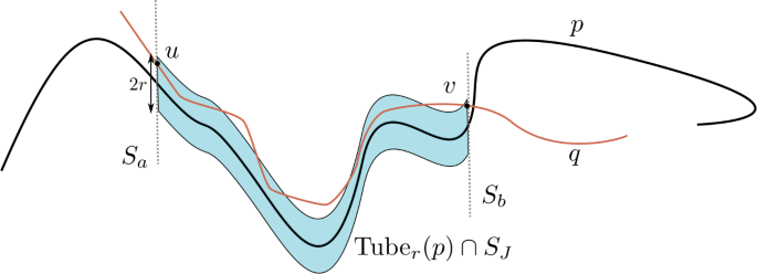

  

  Illustration of the event that the path q is r-close to the path p on the interval J. The blue region depicts Tube_r(p)∩S_J. This event will be used in the attractive geodesics proposition, Proposition 1.7, where p will have length of order L and J will have length of order m. Color figure online.

The proposition below states that a geodesic is attractive with high probability, provided that it satisfies the following technical requirement of bounded slope: For ρ,m>0, we say that a finite path p in $\mathbb{Z}^{2}$ has (ρ,m)-bounded slope if for all x₁,x₂∈X(p) satisfying |x₁−x₂|≥m it holds that |f_p(x₁)−f_p(x₂)|≤ρ|x₁−x₂|. In words, the slope of p between its pioneer points is bounded above by ρ for every pair of pioneer points with horizontal separation at least m. This requirement is discussed further following the statement of the proposition.

Proposition 1.7

Attractive Geodesics

Suppose G satisfies (EXP) and (ABS). Let ρ>0. There exist C_ρ,c_ρ>0 and 0<α_ρ≤1, depending only on G and ρ, such that the following holds.

Consider the geodesic

$$ \gamma :=\gamma ((0,0),(L,s)) $$

for integer L>0 and s. Let $(I_{i})_{i=0}^{N-1}$ be intervals of the form I_i=[a_i,a_i+1] where 0=a₀<a₁<⋯<a_N=L are integers and with m≤|I_i|≤2m for some m. Define the event

$$ \mathrm{Att}_{r,\xi}:=\left \{ \!\! \textstyle\begin{array}{c} \text{every geodesic which is $r$-close to $\gamma $ on at least $(1-\xi )N$} \\ \text{of the intervals $(I_{i})_{i=0}^{N-1}$ shares an edge with $\gamma $}\end{array}\displaystyle \!\! \right \}. $$

(1.3)

Then

$$ \mathbb{P}\big( (\mathrm{Att}_{r,\xi})^{c}\cap \{ \text{$\gamma $ has $(\rho ,m)$-bounded slope}\} \big) \le C_{\rho }e^{-c_{ \rho}(\log L)^{2}} $$

when

$$ \xi :=\frac{\alpha _{\rho}}{\sqrt{r}\log L} $$

(1.4)

and the parameters satisfy

$$ 1\le r\le \alpha _{\rho}\min \left \{\frac{N}{\log ^{2}L}, \frac{N^{2}}{\log ^{6}L}\right \}\quad \text{and}\quad \max \{r,\log ^{2} L\}\le \alpha _{\rho }\sqrt{\frac{m}{r}}. $$

(1.5)

In our application, the parameters r,N,m will be chosen as suitable powers of L, so that, in particular, assumption (1.5) is satisfied.

To deduce from the proposition that geodesics are typically attractive, we need to prove that they typically have (ρ,m)-bounded slope. This is handled by the next result, for which we require the following limit shape assumption,

For horizontal geodesics (in the sense of (1.8) below), the assumption may be waived.

Proposition 1.8

Suppose G satisfies (EXP), (ABS) and (Nℓ₁). Let δ>0. There exist C,c,ρ>0, depending only on G, and C_δ>0, depending only on G and δ, such that the following holds. Consider the geodesic

$$ \gamma :=\gamma ((0,0),(n,s)) $$

for integer n>0 and s. Assume the ‘at most 45-degree slope’ condition

$$ |s|\le n. $$

(1.6)

Then, for all $m\ge C_{\delta }n^{\frac{1}{2}+\delta}$,

$$ \mathbb{P}\big( \text{$\gamma $ does not have $(\rho ,m)$-bounded slope}\big) \le Ce^{-c( \log n)^{2}}\,. $$

(1.7)

Moreover, if

$$ m\ge |s|+\sqrt{n} \log ^{2} n $$

(1.8)

then (1.7) holds also without the assumption (Nℓ₁).

We can relax the restriction (1.6) (to at most 90−δ degree slope) with extra limit shape assumptions. The proof under condition (1.8) (without assumption (Nℓ₁)) uses only the convexity and the lattice symmetries of the limit shape.

We make several remarks regarding the results of this section.

First, the notion of attractive geodesic is not invariant to rotations of $\mathbb{Z}^{2}$, as the x-axis plays a special role in the definition of r-closeness (the interval J in its definition should be thought of as a subset of the x-axis). We can thus define a notion of “vertically attractive geodesic” by exchanging the role of the x and y axes in our definitions, and our statements will apply just as well for this notion. This fact is especially relevant for the 45-degree assumption (1.6) as one sees that if this assumption is not satisfied by γ, then it will be satisfied once the x and y axes are exchanged. In this sense (1.6) is not a serious restriction. In the proofs of Theorem 1.1 and Theorem 1.4, thanks to this symmetry of the lattice, we can assume without loss of generality that the geodesic satisfies the 45-degree assumption.

Proposition 1.8 ensures that the geodesic does not make “big jumps” with high probability so that, in particular, any sub-path of the geodesic does not make “big jumps”. In the proof of Theorem 1.1, we apply Proposition 1.8 to the whole geodesic, and then apply Proposition 1.7 to suitable sub-paths of the geodesic near its endpoints in order to prove that these sub-paths are typically attractive for suitable choices of r and m.

A second related observation is that if one first rotates the $\mathbb{Z}^{2}$ lattice by 45 degrees, thus making the line y=−x into the new x-axis, one obtains yet another notion of attractive geodesic (where the interval J in the definition of r-closeness should be thought of as a subset of the line y=−x in the original coordinate system). The proofs of our propositions apply also in this rotated coordinate system. It is then worthwhile to note that if the limit shape in the original coordinate system was a dilation of the ℓ₁ ball then after the rotation the limit shape will be a dilation of the ℓ_∞ ball, allowing to apply Proposition 1.8. In this sense, a version of our results holds without need to verify assumption (Nℓ₁). This observation is used in our proof of Theorem 1.4 in order to obtain the result without explicit limit shape assumptions.

1.3 Overview of the proofs

We briefly explain here how some of our main theorems are proved.

Theorem 1.1 shows that geodesics which start near (0,0) and end near a point $y\in \mathbb{Z}^{2}$ will coalesce with high probability. We prove it using a trapping strategy, showing that all such geodesics stay, with high probability, between two reference coalescing geodesics γ⁺ and γ⁻, thereby forcing the coalescence event by the planar geometry (see Fig. 3). The reference geodesic γ⁺ (γ⁻) starts and ends at a suitably chosen distance h above (below) (0,0) and y. For the reference geodesics to form a trap, we need to ensure that they stay ordered, meaning that γ⁺ is always above γ⁻ (in a suitable sense), and that they stay away from the neighborhoods of (0,0) and y. We prove that these properties are satisfied with high probability, when h is somewhat large, using our assumptions on the limit shape (see Proposition 3.1). The coalescence of the reference geodesics is proved using the attractive geodesics proposition, applied to sub-geodesics of γ⁻ of length L≪∥y∥ located at the extremities of γ⁻: To this end, first, Proposition 1.8 is used to verify that the reference geodesics have bounded slope with high probability (assuming WLOG that γ⁻ satisfies the ‘45-degree slope’ condition as in the first remark after Proposition 1.8). Second, the planar geometry, translation invariance of the lattice and the fact that the reference geodesics remain ordered are used to prove that for r≫h, using Markov’s inequality, the reference geodesics are r-close to each other above each segment with high probability.

Figure 3

Illustration of the proof of Theorem 1.1.

Theorem 1.2 shows that the probability of the event $E_{z}^{u,v}$ that a vertex z lies on the geodesic between the vertices u and v is small, when z is separated from u and v. The theorem is deduced from the coalescence result, Theorem 1.1, using an averaging trick (see Fig. 4) as used in the later proofs of the BKS-type concentration bound by Damron–Hanson–Sosoe [DHS15]. Translation invariance of the lattice shows that the probability of $E_{z}^{u,v}$ equals the probability of $E_{z+w}^{u+w,v+w}$ for every w. This gives, in particular, that

(1.9)

where Λ_ℓ is a discrete square of side length ℓ. For w∈Λ_ℓ, with ℓ suitably small, Theorem 1.1 shows that all geodesics of the form γ(u+w,z+w) coalesce and all geodesics of the form γ(z+w,v+w) coalesce, with high probability. When this happens, then all geodesics of the form γ(u+w,v+w) for which $E_{z+w}^{u+w,v+w}$ occurs (with w∈Λ_ℓ) must coincide on the box z+Λ_ℓ. Therefore, on this event, the quantity inside the expectation in (1.9) does not exceed the order $\frac{1}{\ell}$ (with high probability, since geodesics only spend order ℓ time in z+Λ_ℓ), yielding the required bound.

Figure 4

Illustration of the proof of Theorem 1.2.

The highways and byways result of Theorem 1.4 is deduced directly from the attractive geodesics proposition, Proposition 1.7, without relying on the coalescence result of Theorem 1.1. It is first noted that if two geodesics which start at the origin follow non-identical paths in Λ_n, then their continuations as they exit Λ_n must be disjoint (since there is a unique geodesic between every two points). However, by the attractive geodesics proposition, disjoint geodesics cannot be close to each other for a long time. Consequently, due to planarity and the limited area in the annulus Λ_4n∖Λ_n, it follows that most pairs of geodesics starting at the origin and heading in a similar direction must not separate before exiting Λ_n. As noted above, no explicit limit shape assumption is used in the proof - while assumption (Nℓ₁) is used in the proof of Proposition 1.8 (and the conclusion of Proposition 1.8 is needed when applying the attractive geodesics proposition), the assumption may be avoided by also considering 45-degree rotations of the $\mathbb{Z}^{2}$ lattice.

The main idea in the proof of Theorem 1.5 is to take advantage of the fact that in some directions there are more deterministic paths of a given length. For example, there is a unique path of length 2n from (0,0) to (2n,0) while there are $\binom{2n}{n}$ paths of length 2n from (0,0) to (n,n). We also use the fact that the weight distribution is a small perturbation of a constant in order to argue that the geodesics are close to being shortest paths in the graph $\mathbb{Z} ^{2}$. Using this, we prove that two directions which are not very close cannot be on the same flat edge of the limit shape.

The proof of the attractive geodesics proposition in Sect. 2 starts with a main steps part (Sect. 2.1) which may serve as an overview of it. Among the ingredients in the proof is a Mermin–Wagner style argument which is explained in Sect. 2.3.

1.4 Discussion, extensions and open problems

1.4.1 Coalescence of geodesics

Theorem 1.1 proves that geodesics of length n whose starting and ending points are at distance h=n^1/8−ϵ coalesce with high probability. We briefly review here the literature on similar results.

The most progress has been achieved for “exactly-solvable models”: Directed last-passage percolation models (in two dimensions) for which exact formulas have been found for the basic statistics. In these models the exponent 2/3 was shown to govern the coalescence (as is also predicted for first-passage percolation). The first result is due to Wütrich [Wut02] who proved that with high probability geodesics will not coalesce at distance h=n^2/3+ϵ. This was later improved by Pimentel [LP16] to show that the geodesics will not coalesce with uniformly positive probability when h=Cn^2/3 for any C>0. Basu, Sarkar and Sly [BSS19] proved that 2/3 is the right exponent by showing that geodesics at distance Cn^2/3 will coalesce with probability tending to 1 as C↓0. Zhang [Zha20], and independently Balázs, Busani and Seppäläinen [BBS21] and Seppäläinen and Shen [SS20] improved the quantitative bounds and estimated the probability of coalescence up to constants as C→0 and as C→∞. See also [SS21, BSS19, Sep20, SS21, BGH22] for the study of infinite geodesics in exactly-solvable models.

In the first-passage percolation setting there are no quantitative and unconditional coalescence results such as Theorem 1.1 (taking into account Theorem 1.5). In fact, the only quantitative result we are aware of is that of Alexander [Ale20] who obtained statements with precise exponents, but under strong assumptions which are currently proved only in the exactly-solvable models (in particular, they are not known to hold for any weight distribution in the first-passage percolation setting). A non-quantitative coalescence result was proved by Licea and Newman [LN96, New95] for infinite geodesics (semi-infinite paths for which every finite sub-path is a geodesic) in two dimensions. They showed that for almost all directions θ∈[0,2π), any two infinite geodesics with asymptotic direction θ must coalesce. Their results were strengthened by Damron–Hanson [DH14] and Ahlberg–Hoffman [AH19]: For θ∈[0,2π) denote by v_θ the unique point in $\partial \mathcal {B}_{G}$ in the direction θ. Damron–Hanson proved that in two dimensions, for any direction θ∈[0,2π) such that the limit shape is differentiable at v_θ, there exist no disjoint infinite geodesics with θ as a direction. Ahlberg–Hoffman developed an ergodic theory of random coalescing geodesics in dimension 2. They proved that the properties of coalescence described in [DH14] are not only valid for some geodesics but are in some sense valid for a dense set of geodesics. The results of [DH14, AH19] are also non-quantitative, but have the advantage of applying to the more general setup of ergodic edge weights.

We further refer to [New97, Weh97, WW98, Hof05, Hof08, DH14, ADH15, DH17, JRS19, Sch21, SS22, ES22] and the survey [ADH17] for additional results on the geometry of geodesics in first- and last-passage percolation.

An interesting direction for extending Theorem 1.1 is to prove a quantitative coalescence result for infinite geodesics. To this end, one would naturally need a coalescence result in which the distance to coalescence does not depend on the overall length of the geodesics. The following is an example of such a statement: Let γ_n,h be the geodesic from (0,0) to (n,h). Prove that for some C>0 depending on G, universal α₁,α₂>0 and all h,n>0,

$$ \mathbb{P}(|\gamma _{n,0}\triangle \gamma _{n,h}|\ge h^{\alpha _{1}}) \le Ch^{-\alpha _{2}}. $$

(1.10)

The obstacles in adapting our argument to prove (1.10) are to control the vertical fluctuations of the geodesics (as in Proposition 1.8) and to create suitable ‘traps’ for the geodesics as in Sect. 3. We believe these may be overcome by relying on stronger limit shape assumptions than those in Theorem 1.1 but have not pursued this extension here.

1.4.2 The influence of edges

As previously mentioned, the works of Damron–Hanson [DH14] and Ahlberg–Hoffman [AH19] provided a non-quantitative resolution of the BKS midpoint problem. In addition, the aforementioned work of Alexander [Ale20] provided quantitative bounds for the BKS problem under strong assumptions which are currently known to hold only in the exactly-solvable models.

The exponent 1/16 in Theorem 1.2 follows from optimizing between the different parameters in our proof. The correct exponent is expected to be 2/3, the same as the exponent predicted to govern the transversal fluctuations of geodesics.

Theorem 1.2 can be seen as a bound on the “first-order influence of edges” in the sense that it bounds the probability that a single given edge is in the geodesic. It is natural to ask also about “higher-order influences” in the sense of asking about the probability that several edges are simultaneously in the geodesic. In this direction, we offer the following natural problem: Does the correlation between the choices of first and last edges in the geodesic from (0,0) to (n,0) tends to zero as n→∞?

It is conjectured that in two-dimensional first-passage percolation there are no infinite bigeodesics, at least when the edge weight distribution G is continuous (the problem originates from Furstenberg; see [Kes86, (9.22)]). This has been rigorously established in some of the exactly-solvable last-passage percolation models [BBS20, BHS22, SS21, GJR21]. In first-passage percolation, Alexander [Ale20] proved the non-existence of bigeodesics in all dimensions d≥2 under the strong assumptions mentioned above. Under an assumption on G and on the curvature of the limit shape, Newman [New95] proved that any infinite geodesic admits almost surely an asymptotic direction. Licea and Newman [LN96, New95] rule out the existence of bigeodesics with both ends in fixed directions (outside a set of null measure) in two dimensions. Their results are strengthened by Damron–Hanson [DH14] and Ahlberg–Hoffman [AH19]: they proved that in two dimensions, for any direction θ∈[0,2π) such that the limit shape is differentiable at v_θ, there exist no infinite bigeodesics with θ as a direction.

1.4.3 Highways and byways

Besides the work of Ahlberg–Hanson–Hoffman [AHH22] mentioned above, we are aware of only one earlier study of upper bounds in the highways and byways problem. Coupier [Cou18] considers a class of random trees embedded in $\mathbb{R}^{2}$ and studies the number of intersection points of a large circle around the origin with semi-infinite paths in the tree. His framework covers both the tree of first-passage paths starting at the (closest point to the) origin in the isotropic, Poisson-process based, first-passage percolation model of Howard and Newman [HN97] and the tree of last-passage paths from the origin in directed last-passage percolation on the lattice. In both cases, Coupier obtains a non-quantitative upper bound on the number of intersections, of a similar flavor to that obtained by Ahlberg–Hanson–Hoffman, with the bound in the directed last-passage percolation case proved under the assumption that the limit shape is strictly concave and differentiable. Coupier further discusses a random tree of a very different nature, formed by local rules. For this tree, which he terms radial Poisson tree, a quantitative, power-law upper bound on the number of intersections is obtained.

1.4.4 Limit shape properties

Theorem 1.5 proves that the limit shape has many sides for a particular class of distributions. We are only aware of few related results in the literature, as we now describe.

Damron–Hochman [DH13], relying on results of Marchand [Mar02] and Kesten [Kes86], construct an atomic distribution whose limit shape has an infinite number of sides.

Basdevant–Gouéré–Théret [BGT21] determined the first-order behavior of the limit shape corresponding to the weight distribution Bernoulli(1−ϵ) as ϵ tends to 0. Using their result one can show that the number of extreme points of the limit shape corresponding to Bernoulli(1−ϵ) tends to infinity as ϵ↓0.

1.4.5 Related models

Analogs of our main results (Theorem 1.1, Theorem 1.2 and Theorem 1.3) continue to hold for point-to-line geodesics (i.e., geodesics from nearby starting points to the same line will coalesce with high probability), requiring only notational modifications in the proof.

The proofs of our main results should also extend, with minimal changes, to directed first- and last-passage percolation models in a planar geometry (under the added condition that the slope between the starting and ending points of the geodesics under study is bounded away from the maximal and minimal allowed slopes). In fact, the proofs should simplify in this setting, since if a directed geodesic starts and ends above another directed geodesic then they must deterministically preserve their order throughout.

Lastly, one may also consider first-passage percolation in the “slab” S_[0,n] for some integer n>0 (this may be thought of as first-passage percolation on $\mathbb{Z}^{2}$ in which the weights of the edges not fully contained in S_[0,n] are set to infinity). Analogs of our main results can also be proved in this setting, with minimal modifications to our proofs, for geodesics connecting the sides of the slab (i.e., starting at (0,y₁) and ending at (n,y₂) for some y₁,y₂). Similarly to the directed models, geodesics connecting the sides of the slab deterministically preserve their ordering in this setting. The lower bound on the required number of sides of the limit shape in this setting stems solely from the analog of Proposition 1.8, so the coalescence result should hold without any limit shape assumptions in the case of horizontal geodesics (i.e., geodesics satisfying (1.8)).

1.4.6 Higher dimensions and minimal surfaces

For first-passage percolation on $\mathbb{Z}^{d}$ with dimension d≥3, Proposition 1.7 remains true with minimal change to the proof, as long as condition (1.5) is suitably modified. Among other things, the new condition needs to imply that the “cost” to connect two geodesics separated by distance r, which is of order r in the way we argue (in any dimension), is smaller than the increase generated by the Mermin–Wagner style argument (Sect. 2.3)), which is of order $\sqrt{m/r^{d-1}}$.

However, planarity is crucially used in the proof of Theorem 1.1 to keep the ordering between the geodesics (i.e., to show that if a geodesic has its endpoints above those of another geodesic then it will very likely remain above the other geodesic throughout). Ordering, in turn, is used to ensure (using Markov’s inequality) that geodesics with nearby starting and ending points spend significant time near each other with high probability (so that Proposition 1.7 is applicable). As the ordering is lost in dimensions d≥3, we do not know how to apply Proposition 1.7 in order to deduce coalescence.

We mention that while the BKS midpoint problem is open in dimensions d≥3, partial results are available [DEP23] as well as results under assumptions which are still unverified [Ale20].

The above regards first-passage percolation on $\mathbb{Z}^{d}$ for d≥3. There is also a different extension of first-passage percolation to higher dimensions, in which “time” is taken to be higher dimensional. In this version the object of study is a minimal surface in a random environment. Such minimal surfaces model the domain walls in the disordered ferromagnet (the random-bond Ising model); see [BGP23, Sect. 1.1] and [D+24, Sect. 1.4] for background and [DG24, BGP23, D+24] for recent work on transversal and ground energy fluctuations. The problems of coalescence and midpoint delocalization make sense also in this context and would be interesting to explore.

1.4.7 The assumptions

The assumption (EXP) is used to ensure that the probability that the passage time between $u,v\in \mathbb{Z}^{2}$ is larger than ρ∥u−v∥, for some constant ρ>0, is exponentially small in ∥u−v∥ (see Claim 2.9). Weaker decay rates may also suffice in our arguments.

The second assumption (ABS) is mostly used in Claim 2.14 as part of the proof of our Mermin–Wagner style result. It may be possible to push our arguments to a class of non absolutely-continuous distributions but we have not attempted to do so.

The assumed lower bound on the number of sides of the limit shape is required in order to have sufficient control on the geometry of geodesics to produce the “traps” used in the proof of Theorem 1.1. In particular, we want to ensure that a geodesic that has endpoints far above another geodesic is unlikely to go below that other geodesic.

1.5 Reader’s guide

The rest of the paper is organized as follows. In the next section we prove Proposition 1.7, which is the main technical ingredient in our proofs. Theorem 1.1, Theorem 1.2, Theorem 1.3 and Theorem 1.4 are then deduced in Sect. 3. The first three of these theorems further require control on the amount of time that a geodesic spends “going in a wrong direction”, as stated in Proposition 3.1. This control is achieved in Sect. 4 where we study the geometry of geodesics and prove Proposition 1.8 and Proposition 3.1 using our assumptions on the limit shape. Finally, in Sect. 5 we establish the lower bound on the number of sides of the limit shape given in Theorem 1.5. The latter proof is independent of the rest of the paper.

2 Proof of the attractive geodesics proposition

In this section we prove Proposition 1.7. We assume that L is sufficiently large for the arguments (as a function of the distribution G and the parameter ρ) as the constants in the proposition may be adjusted to fit smaller L. We also assume throughout that G satisfies (EXP) and (ABS) and we continue with the notation of the proposition.

2.1 Main steps

In this section we give an overview of the proof of the proposition, postponing the proofs of some of the intermediate steps to later sections.

2.1.1 Attractive intervals

Consider the geodesic

$$ \gamma :=\gamma ((0,0),(L,s)) $$

for integer L>0 and s. Call an interval J⊂[0,L] with integer endpoints attractive if every geodesic which is r-close to γ on J necessarily has an edge in common with γ. The following containment of events is immediate,

(2.1)

We thus focus on giving a lower bound for the probability of the left-hand side event. As the first step we develop a sufficient condition for an interval to be attractive.

The following basic bound, controlling the passage time and length of geodesics, will be helpful.

Lemma 2.1

There exist C,c,ρ₁,ρ₂>0, depending only on G, such that the following holds. Let Ω_basic be the event that for all $u,v\in [-L^{2},L^{2}]^{2}\cap \mathbb{Z}^{2}$ it holds that

$$ T(u,v)\le \rho _{1}\max \{\|u-v\|_{1},\log ^{2} L\}\quad \text{and} \quad |\gamma (u,v)|\le \rho _{2}\max \{\|u-v\|_{1},\log ^{2} L\}, $$

(2.2)

where we write |p| for the number of edges in a path p. Then

$$ \mathbb{P}(\Omega _{\mathrm {basic}})\ge 1 - Ce^{-c\log ^{2} L}. $$

The lemma is proved in Sect. 2.2. The notation ρ₁,ρ₂ is reserved throughout our argument to the constants from the lemma.

To make use of the lemma for the geodesic γ, we first note that when γ has (ρ,m)-bounded slope then |f_γ(L)|≤ρL. Thus, as we’ve assumed that L is large as a function of ρ, the subgeodesic of γ between (0,0) and (L,f_γ(L)) satisfies the estimates (2.2).

Let

$$ \mathcal{P}:=\{p\colon \text{$p$ is a path in $\mathbb{Z}^{2}$ with $\mathbb{P}(\gamma =p)>0$}\}, $$

so that, in particular, each $p\in \mathcal{P}$ is a path from (0,0) to (L,s) and $\gamma \in \mathcal{P}$ almost surely.

Let J=[a,b]⊂[0,L] be an interval with integer endpoints and $p\in \mathcal{P}$. Write

$$ T_{p}(J):=T((a,f_{p}(a)), (b,f_{p}(b))) $$

for the passage time from the pioneer point of p above a to the pioneer point of p above b (using the geodesic between these two points, which may differ from p).

A central role in our analysis is played by the following notion of the restricted passage time $\bar{T}_{p}(J)$, defined as the minimal passage time among (simple) paths q satisfying

• (1) q is edge-disjoint from p.

• (2) One endpoint of q is in Tube_r(p)∩S_a and the other is in Tube_r(p)∩S_b.

• (3) The number of edges of q with both endpoints in Tube_r(p)∩S_J is at least $\frac{1}{2}|J|$.

• (4) |q|≤ρ₂max{∥u−v∥₁,log²L} where u and v are the endpoints of q.

(setting $\bar{T}_{p}(J):=\infty$ if no such path exists). The set of paths satisfying these properties is denoted by Q_p(J).

The following is our sufficient condition for the attractiveness of J: Let

$$ \Omega (J):=\{\bar{T}_{\gamma}(J)> T_{\gamma}(J)+2\rho _{1} \max \{r, \log ^{2} L\}\}. $$

(2.3)

Then

$$\begin{aligned} &\text{on $\Omega (J)\cap \Omega _{\mathrm {basic}}\cap \{\gamma $ has $(\rho ,m)$\text{-bounded slope}$\}$} \\ &\text{it holds that $J$ is attractive}. \end{aligned}$$

(2.4)

Let us prove this. Assume Ω_basic and assume that γ has (ρ,m)-bounded slope. We show that the existence of a geodesic γ′ which is r-close to γ on J and is edge-disjoint from γ implies that Ω(J) does not occur. First, it follows from the properties of γ′ that it contains a subgeodesic γ″ connecting some (a,y₁)∈Tube_r(γ)∩S_a to some (b,y₂)∈Tube_r(γ)∩S_b which satisfies properties (1),(2),(3) above with q=γ″ and p=γ. Moreover, we claim that γ″ also satisfies property (4) so that it belongs to Q_γ(J). This follows from Ω_basic, as the endpoints of γ″ are in [−L²,L²]² by our upper bound (1.5) on r (with α_ρ≤1, say) and since γ has (ρ,m)-bounded slope. Second, since γ″ is a geodesic, its passage time must be at most that of the path going along the geodesic from (a,y₁) to (a,f_γ(a)), then along γ from (a,f_γ(a)) to (b,f_γ(b)) and finally along the geodesic from (b,f_γ(b)) to (b,y₂). On Ω_basic, the latter path has passage time at most T_γ(J)+2ρ₁max{r,log²L}. Since $\bar{T}_{\gamma}(J)\le T(\gamma '')$, we conclude that Ω(J) does not hold.

With the sufficient condition (2.4) in hand, and taking into account the containment (2.1) and Lemma 2.1, we see that Proposition 1.7 follows from the following statement: There exist C_ρ,c_ρ>0, depending only on G and ρ, such that

(2.5)

The next sections present the proof of this estimate, which relies on the following ingredients:

• (1) An upper bound for the passage time T_γ(I_i) of many of the intervals (I_i). The main observation here is that Talagrand’s concentration inequality self-improves when applied to sub-geodesics of γ due to the concavity of the square root function.

• (2) A lower bound for the probability that a restricted passage time $\bar{T}_{p}(I_{i})$ is long. This uses a Mermin–Wagner style argument (perturbing the edge passage times) to obtain lower bounds on the fluctuations of $\bar{T}_{p}(I_{i})$.

• (3) The Harris correlation inequality for monotonic events in independent variables.

2.1.2 The passage time of γ on many of the intervals I _i is short

For $u,v\in \mathbb{Z}^{2}$, write

$$\begin{aligned} E(u,v) &:= \mathbb{E}[T(u,v)], \\ D(u,v) &:= T(u,v) - E(u,v) \end{aligned}$$

for the expected passage time between u and v and the deviation from the expectation. We may note that E is a (deterministic) metric on $\mathbb{Z}^{2}$, since T is a (random) metric on $\mathbb{Z}^{2}$. Talagrand’s concentration inequality provides the following control on D(u,v).

Lemma 2.2

There exist C,c>0, depending only on G, such that the following holds. Let Ω_Tal be the event that for all $u,v\in [-L^{2},L^{2}]^{2}\cap \mathbb{Z}^{2}$,

$$ |D(u,v)|\le \sqrt{\|u-v\|_{1}}\log L. $$

(2.6)

Then

$$ \mathbb{P}(\Omega _{\mathrm {Tal}})\ge 1 - Ce^{-c\log ^{2} L}. $$

The lemma is proved in Sect. 2.2.

The observation made in this section, stated in (2.8) below, is that (2.6) may be improved ‘on average’ for sub-geodesics of γ due to the concavity of the square root function.

For an interval J=[a,b]⊂[0,L] with $a,b\in \mathbb{Z}$ and a path $p\in \mathcal{P}$, let

$$ E_{p}(J):=E((a,f_{p}(a)), (b,f_{p}(b))) $$

be the expected passage time between the pioneer points of p above the endpoints of J. We think of E_p(J) as a deterministic function of the path p and when we write E_γ(J) we simply substitute the random path γ inside this function (so that E_γ(J) is a random variable, different from the deterministic quantity $\mathbb{E}[T_{\gamma}(J)]$). Define p[J] to be the subpath of p between the points (a,f_p(a)) and (b,f_p(b)), and define

$$ D_{p}(J):=T(p[J])-E_{p}(J) $$

(2.7)

where the time of a path was defined in (1.1). Note that T_γ(J)=T(γ[J]) almost surely as γ is a geodesic. The quantity D_γ(J) is a measure of the deviation of the passage time of the sub-geodesic of γ between the pioneer points at a and b.

It is straightforward to check that the following statements hold almost surely,

$$\begin{aligned} &T_{\gamma}([0,L])=\sum _{i=0}^{N-1} T_{\gamma}(I_{i}), \\ &E_{\gamma}([0,L]) \le \sum _{i=0}^{N-1} E_{\gamma}(I_{i}) \end{aligned}$$

(the inequality follows since E(⋅,⋅) is a metric). Consequently,

$$ \sum _{i=0}^{N-1} D_{\gamma}(I_{i})\le D_{\gamma}([0,L]) = D((0,0),(L,f_{ \gamma}(L)))\quad \text{almost surely}. $$

(2.8)

We conclude that on Ω_Tal∩{γ has (ρ,m)-bounded slope},

$$ \sum _{i=0}^{N-1} D_{\gamma}(I_{i})\le \sqrt{(1+\rho )L}\log L\quad \text{and}\quad \min _{0\le i\le N-1} D_{\gamma}(I_{i})\ge -\sqrt{2m(1+ \rho )}\log L. $$

(2.9)

The assertion (2.9) is harnessed in the following way. It is straightforward that if (2.9) holds then for each τ satisfying

$$ \tau \ge \frac{\sqrt{(1+\rho )L}\log L}{N} $$

(2.10)

we have that either Ω_1,τ or Ω_2,τ occurs, with

(2.11)

(2.12)

We will use this conclusion with $\tau = \sqrt{\frac{m}{r}}$, noting that (2.10) is satisfied due to our assumption (1.5) (choosing α_ρ sufficiently small). For a path $p\in \mathcal{P}$, it will be convenient to denote by Ω_1,τ(p) and Ω_2,τ(p) the events appearing in (2.11) and (2.12), respectively, in which all occurrences of D_γ(I_i) are replaced by D_p(I_i).

2.1.3 The restricted passage time is long with non-negligible probability

In this section we provide lower bounds for the probability that a restricted passage time $\bar{T}_{p}(I_{i})$ is long and further discuss the independence properties of the restricted passage times.

Lemma 2.3

There exists c_ρ>0, depending only on G and ρ, such that the following holds. For each path $p\in \mathcal{P}$ having (ρ,m)-bounded slope, each 0≤i≤N−1 and each $5\rho _{1} \max \{r,\log ^{2} L\}\le t\le \sqrt{2m(1+\rho )}\log L$,

$$\begin{aligned} &\mathbb{P}\left (\bar{T}_{p}(I_{i})\ge E_{p}(I_{i}) - t+2\rho _{1} \max \{r,\log ^{2}L\}\right )\ge \frac{c_{\rho }t}{\sqrt {m}\log L}, \end{aligned}$$

(2.13)

$$\begin{aligned} &\mathbb{P}\left (\bar{T}_{p}(I_{i})\ge E_{p}(I_{i}) + 6\sqrt{ \frac{m}{r}}+2\rho _{1} \max \{r,\log ^{2} L\}\right )\ge \frac{c_{\rho}}{\sqrt{r}\log L}. \end{aligned}$$

(2.14)

The proof of Lemma 2.3, relying on Talagrand’s concentration inequality, is given in Sect. 2.2. The proof of (2.14) additionally uses a “Mermin–Wagner style argument” developed in Sect. 2.3. On an intuitive level, the argument yields that the distribution of $\bar{T}_{p}(I_{i})$ “contains a Gaussian component with variance of order $\frac{m}{r}$” (see Lemma 2.17 for the precise result). This implies the following statement.

Lemma 2.4

Let $p\in \mathcal{P}$ have (ρ,m)-bounded slope and let J⊂[0,L] be an interval with integer endpoints satisfying m≤|J|≤2m. There exist C_ρ,c_ρ>0, depending only on G and ρ, such that for each $0\le \alpha \le c_{\rho}\sqrt{m r}$ and each real a,

$$ \sqrt{\mathbb{P}\left (\bar{T}_{p}(J)\ge a+\alpha \sqrt{\frac{m}{r}} \right )}\ge e^{-C_{\rho}\alpha ^{2}} \big( \mathbb{P}\left (\bar{T}_{p}(J) \ge a\right ) - e^{-m}\big) . $$

The argument leading from Lemma 2.4 to the inequality (2.14) is explained in Sect. 2.2.

We remark that the “standard deviation lower bound $\sqrt{\frac{m}{r}}$” is obtained as the ratio between the length of J and the square root of the volume of the r-tube of p above J (using in the process that paths in Q_p(J) must spend a significant fraction of their time in the r-tube). This is of the same nature as the relation $\chi \ge \frac{1 - (d-1)\xi}{2}$ on $\mathbb{Z}^{d}$, between the fluctuation exponent χ and transversal exponent ξ, obtained by Wehr–Aizenman [WA90, Sect. 6] and Newman–Piza [NP95, Theorem 5]. Our arguments may also be used to obtain such a relation.

We also remark that it would have been helpful to know the natural fact that T_p(I_i)≥E_p(I_i) occurs with probability bounded away from zero uniformly in L,m,r. Such a fact would both simplify and lead to better probability lower bounds in Lemma 2.3.

Recall that our goal is to prove the probability bound (2.5). This requires showing that several of the restricted passage times $\bar{T}_{\gamma}(I_{i})$ are simultaneously large. To this end, the following independence property is handy: Set ρ₃:=2ρ₂(1+ρ). For each $p\in \mathcal {P}$ and subset $\mathcal{I}\subset \{0,1,\ldots , N-1\}$,

$$ \text{if $|i_{1}-i_{2}|\ge 2\rho _{3}$ for all distinct $i_{1},i_{2}\in \mathcal{I}$ then }\left (\bar{T}_{p}(I_{i})\right )_{i \in \mathcal{I}}\text{ are independent}. $$

(2.15)

Indeed, recall that $\bar{T}_{p}(I_{i})$ is the minimal passage time among the paths in Q_p(I_i), and that the paths q∈Q_p(I_i) have endpoints with x coordinates a_i and a_i+1 and satisfy

$$ |q|\le \rho _{2}((a_{i+1} - a_{i} )(1+\rho )+2r)\le \rho _{3}(a_{i+1}-a_{i}) $$

(using here that a_i+1−a_i≥m≥log²L and 2r≤m≤a_i+1−a_i by (1.5) with α_ρ≤1). Such paths q thus stay in the slab $S_{[a_{i} - \alpha ,\, a_{i+1} + \alpha ]}$ with $\alpha = \frac{1}{2}(\rho _{3}-1)(a_{i+1}-a_{i})\le (\rho _{3}-1)m$. Thus, $\bar{T}_{p}(I_{i})$ is measurable with respect to the weights of the edges with both endpoints in $S_{[a_{i} - (\rho _{3}-1) m,\, a_{i+1}+(\rho _{3}-1) m]}$, from which (2.15) follows as edges have independent weights. Lemma 2.3 and the independence property (2.15) will be used in the following way. For a path $p\in \mathcal{P}$ having (ρ,m)-bounded slope and a vector of reals $d = (d_{i})_{i=0}^{N-1}$ define the event

(2.16)

(where we recall from (1.4) that $\xi = \frac{\alpha _{\rho}}{\sqrt{r}\log L}$). The following bounds the probability of $\mathcal{E}_{p,d}$.

Proposition 2.5

If α_ρ is sufficiently small (as a function of G and ρ) then

$$ \mathbb{P}(\mathcal{E}_{p,d})\le e^{-\frac{1}{4} \xi N} $$

when

$$ \begin{aligned} &\text{either}\;\;\left |\left \{0\le i\le N-1\colon d_{i} \le 6\sqrt{\frac{m}{r}}\right \}\right |\ge \frac{1}{2}N\;\; \\ &\text{or}\;\;\sum _{i\colon -\sqrt{2m(1+\rho )}\log L\le d_{i}< -\sqrt{ \frac{m}{r}}} d_{i}\le -\sqrt{\frac{m}{r}}N. \end{aligned} $$

(2.17)

The proof uses the following special case of Chernoff’s bound (see, e.g., [HR90, equation (7)]). Let X₁,…,X_k be independent random variables taking values in {0,1} and write $\mu :=\sum _{i=1}^{k}\mathbb{E}(X_{i})$ for the expectation of their sum. Then

$$ \mathbb{P}\left (\sum _{i=1}^{k} X_{i}\le \frac{1}{2}\mu \right )\le e^{- \frac{1}{8}\mu}. $$

(2.18)

Proof of Proposition 2.5

If the first condition in (2.17) holds then there exists a subset $\mathcal{I}\subset \{0,1\ldots , N-1\}$ such that $d_{i}\le 6\sqrt{\frac{m}{r}}$ for $i\in \mathcal{I}$, |i₁−i₂|≥2ρ₃ for all distinct $i_{1},i_{2}\in \mathcal {I}$ and $|\mathcal{I}|\ge \frac{N}{2\lceil 2\rho _{3}\rceil}$. The variables $(\bar{T}_{p}(I_{i}))_{i\in \mathcal{I}}$ are then independent by (2.15). Thus, by (2.18),

where $\mu _{1}:=\sum _{i\in \mathcal{I}}\mathbb{P}(\bar{T}_{p}(I_{i})\ge E_{p}(I_{i}) + 6\sqrt{\frac{m}{r}}+2\rho _{1} \max \{r,\log ^{2} L\})\ge \frac{c_{\rho }N}{2\lceil 2\rho _{3}\rceil \sqrt{r}\log L}$ by (2.14) and where we use that μ₁≥2ξN when α_ρ is chosen sufficiently small (here c_ρ is the constant from (2.14)).

Similarly, if the second condition in (2.17) holds then there exists $\mathcal{I}\subset \{0,1\ldots , N-1\}$ such that $-\sqrt{2m(1+\rho )}\log L\le d_{i}<-\sqrt{\frac{m}{r}}$ for $i\in \mathcal{I}$, |i₁−i₂|≥2ρ₃ for all distinct $i_{1},i_{2}\in \mathcal {I}$ and $\sum _{i\in \mathcal{I}}d_{i} \le - \frac{1 }{\lceil 2\rho _{3}\rceil}\sqrt{\frac{m}{r}} N$. The variables $(\bar{T}_{p}(I_{i}))_{i\in \mathcal{I}}$ are again independent by (2.15). Thus, by (2.18),

where

$$\begin{aligned} \mu _{2}&=\!\sum _{i\in \mathcal{I}}\mathbb{P}(\bar{T}_{p}(I_{i})\ge E_{p}(I_{i}) + d_{i} +2\rho _{1} \max \{r,\log ^{2} L\})\!\ge \! \frac{c_{\rho }}{\sqrt{m}\log L}\!\sum _{i\in \mathcal{I}}|d_{i}|\! \\ &\ge \!\frac{c_{\rho }N}{\lceil 2\rho _{3}\rceil \sqrt{r}\log L} \end{aligned}$$

by (2.13) (checking that $\sqrt{\frac{m}{r}}\ge 5\rho _{1}\max \{r,\log ^{2}L\}$ by (1.5) when α_ρ is sufficiently small), and where we use that μ₂≥2ξN when α_ρ is sufficiently small (here c_ρ is the constant from (2.13)). □

2.1.4 Monotonic events

Recall that Harris’ inequality (generalized to dependent variables by the FKG inequality) states that two increasing events in independent random variables are non-negatively correlated [Har60]. In this section we explain the use that we make of this inequality in our context.

Let $p\in \mathcal{P}$. Observe that the event {γ=p} is decreasing in the weights (t_e)_e∈p and increasing in the weights (t_e)_e∉p. Thus, by Harris’ inequality, it is non-negatively correlated with every event sharing the same monotonicity properties. We employ the following variant of this observation.

Lemma 2.6

Let $p\in \mathcal{P}$. Let E be an event which is decreasing in the weights (t_e)_e∉p (for every fixed value of (t_e)_e∈p). Then the following inequality of conditional probabilities holds almost surely,

$$ \mathbb{P}\big( \{\gamma =p\}\cap E\,|\,(t_{e})_{e\in p} \big) \le \mathbb{P} \big( \{\gamma = p\}\,|\,(t_{e})_{e\in p} \big) \cdot \mathbb{P} \big(E\,|\,(t_{e})_{e\in p} \big) . $$

(2.19)

Proof

The IID structure of the environment implies that the (t_e)_e∉p remain independent after conditioning on (t_e)_e∈p. As {γ=p} is an increasing event in (t_e)_e∉p while E is decreasing in these variables, we may apply Harris’ inequality in the conditional probability space to obtain (2.19). □

2.1.5 Putting all the ingredients together

In this section we explain how the results of the previous sections are combined to prove (2.5), from which the attractive geodesic proposition, Proposition 1.7, follows. We assume throughout that the constant α_ρ in (1.5) is taken sufficiently small for the arguments.

Write $\mathcal{P}_{\rho ,m}:=\{p\in \mathcal{P}\colon p \text{ has $(\rho ,m)$-bounded slope}\}$. Also set D_p:=(D_p(I_i))_{0≤i≤N−1} (recalling the definition of D_p(J) from (2.7)). First,

with the second equality following by comparing the definition (2.3) of Ω(J), the definition (2.7) of D_p(J) and the definition (2.16) of $\mathcal{E}_{p,d}$, and with the inequality following from Lemma 2.2. Second, for each $p\in \mathcal{P}_{\rho ,m}$,

with the first equality following from the discussion after (2.9) and the second equality following from the definition of Ω_1,τ(p) and Ω_2,τ(p) following (2.12), making use of the intersection with the event {γ=p}. Third, we condition on the passage time of the edges on the path p and observe that D_p and hence also the Ω_i,τ(p) events are measurable with respect to this conditioning. Thus,

where the first inequality follows from Lemma 2.6 (as $\mathcal{E}_{p,D_{p}}$ is decreasing in (t_e)_e∉p, for each fixed value of (t_e)_e∈p) and the second inequality follows from Proposition 2.5 (using the IID structure of the environment, as $\mathcal{E}_{p,d}$ is independent of (t_e)_e∈p while D_p is measurable with respect to these variables), noting that the Ω_i,τ(p) events exactly ensure that condition (2.17) holds.

Putting the previous displayed equations together, we finally conclude that

This concludes the proof of (2.5), and hence of Proposition 1.7, once we note that ξN≥c_ρlog²L by (1.5), for some c_ρ>0 depending only on G and ρ.

2.2 Basic lemmas

In this section we prove that the events Ω_basic (Lemma 2.1) and Ω_Tal (Lemma 2.2) occur with high probability, and also prove Lemma 2.3 using Lemma 2.4.

Lemma 2.2 is deduced from Talagrand’s concentration inequality.

Theorem 2.7

Talagrand’s inequality [Tal95]

There exist C,c>0, depending only on G, such that for all $u,v\in \mathbb{Z} ^{2}$ we have that

$$ \forall t\ge 0:\qquad \mathbb{P} \Big( \left | T(u,v)-\mathbb{E} [T(u,v)] \right | \ge t \sqrt{\|u-v\|_{1}} \Big) \le Ce^{-ct^{2}}. $$

Proof of Lemma 2.2

We have

$$ \Omega _{\mathrm {Tal}}^{c}\subset \bigcup _{u,v\in [-L^{2},L^{2}]^{2}\cap \mathbb{Z}^{2}} \left \{ |T(u,v)-\mathbb{E} [T(u,v)]|>\sqrt{\|u-v\|_{1}}\log L\right \}. $$

The result follows from Theorem 2.7 and a union bound. □

To prove Lemma 2.1, we need the following two claims.

Claim 2.8

There exist C,c,ρ₂>0, depending only on G, such that for every $u,v\in \mathbb{Z} ^{2}$ and n≥ρ₂∥u−v∥₁, we have

$$ \mathbb{P} \big( |\gamma (u,v) |\ge n \big) \le Ce^{-cn}. $$

Claim 2.9

There exist c,ρ₁>0, depending only on G, such that for every $u,v\in \mathbb{Z} ^{2}$ and n≥ρ₁∥u−v∥₁, we have

$$ \mathbb{P} \big(T(u,v)\ge n \big) \le e^{-cn}. $$

Proof of Lemma 2.1

We have

$$ \begin{alignedat}{1} \Omega _{\mathrm {basic}}^{c}\subset \bigcup _{u,v\in [-L^{2},L^{2}]^{2}\cap \mathbb{Z}^{2}} \Big(&\left \{ T(u,v)>\rho _{1}\max \{\|u-v\|_{1},\log ^{2}L\}\right \} \\ &\cup \left \{ |\gamma (u,v)|>\rho _{2}\max \{\|u-v\|_{1},\log ^{2} L \} \right \}\Big). \end{alignedat} $$

The result follows from Claim 2.8, Claim 2.9 and a union bound. □

We proceed to prove the claims.

Proof of Claim 2.9

Let p be a deterministic path between u and v such that |p|=∥u−v∥₁. For instance, one can choose the path that first goes straight in the vertical direction and then straight in the horizontal direction. For each α>0, Markov’s inequality and the independence of the edge weights yield that every n≥ρ₁∥u−v∥₁,

$$ \begin{aligned} \mathbb{P}(T(u,v)\ge n)&\le \mathbb{P}(T(p)\ge n)= \mathbb{P}\left (e^{\alpha T(p)}\ge e^{\alpha n}\right ) \\ &\le \left (\mathbb{E} e^{\alpha t_{e}}\right )^{\|u-v\|_{1}} e^{- \alpha n}\le \left (\left (\mathbb{E} e^{\alpha t_{e}}\right )^{1/ \rho _{1}} e^{-\alpha}\right )^{n}. \end{aligned} $$

The claim follows by choosing α to be the constant from our assumption (EXP) and choosing ρ₁ sufficiently large. □

To prove Claim 2.8 we need the following result due to Kesten, a corollary of Proposition 5.8 in [Kes86].

Theorem 2.10

Suppose the edge-weight distribution G satisfies G({0})<p_c(2) (with p_c(2)=1/2 the critical probability for bond-percolation on $\mathbb{Z}^{2}$). Then there exist C,c,ρ₀>0, depending only on G, such that

$$ \forall n\geq 0: \qquad \mathbb{P} \left ( \textstyle\begin{array}{c} \textit{There exists a (simple) path $q$ starting } \\ \textit{from $(0,0)$ such that $|r|\geq n$ and $T(r)< \rho _{0}n$}\end{array}\displaystyle \right )\leq C\exp (-cn)\,. $$

Proof of Claim 2.8

For each $u,v\in \mathbb{Z}^{2}$ and n>0,

$$ \mathbb{P}(|\gamma (u,v)|\geq n)\le \mathbb{P} \left (\!\!\! \textstyle\begin{array}{c} \text{There exists a (simple) path $q$ starting } \\ \text{from $u$ such that $|r|\geq n$ and $T(r)< \rho _{0}n$}\end{array}\displaystyle \!\!\right )+\mathbb{P}(T(u,v)\ge \rho _{0} n) $$

The claim thus follows from Theorem 2.10 (using translation invariance) and Claim 2.9 with ρ₂:=ρ₁/ρ₀. □

Let us now prove Lemma 2.3. The following preliminary claim shows that $\bar{T}_{p}(J)$ is unlikely to be much smaller than T_p(J).

Claim 2.11

Connection cost

There exist C,c>0, depending only on G, such that the following holds. For each path $p\in \mathcal {P}$ and each interval J=[a,b]⊂[0,L] with integer endpoints,

$$ \mathbb{P} \big( \bar{T}_{p}(J) \ge T_{p}(J) -2\rho _{1}\max \{r,\log ^{2} L\} \big) \ge 1-Ce^ {-c\log ^ {2}L}\,. $$

Proof

By the triangle inequality,

$$ \begin{alignedat}{1} T_{p}(J)&\le \min _{ \substack{u\in \mathrm {Tube}_{r}(p)\cap S_{a}\\v\in \mathrm {Tube}_{r}(p)\cap S_{b}}} T((a,f_{p}(a)),u)+T(u,v)+T(v,(b,f_{p}(b))) \\ &\le \bar{T}_{p}(J)+\max _{u\in \mathrm {Tube}_{r}(p)\cap S_{a}} T((a,f_{p}(a)),u)+ \max _{v\in \mathrm {Tube}_{r}(p)\cap S_{b}}T(v,(b,f_{p}(b))). \end{alignedat} $$

The claim thus follows from Claim 2.9, applied with n=ρ₁max{r,log²L}, and a union bound (using (1.5) with α_ρ≤1). □

Proof of Lemma 2.3, inequality (2.13)

Let J=[a,b]⊂[0,L] be an interval with $a,b\in \mathbb{Z}$ and m≤|J|≤2m. Let $t\in [5\rho _{1} \max \{r,\log ^{2} L\}, \sqrt{2m(1+\rho )}\log L]$. Set X:=T_p(J)−E_p(J). Taking into account Claim 2.11 and the fact that t≥5ρ₁max{r,log²L} we see that it suffices to prove that

$$ \zeta :=\mathbb{P}\left (X\ge -\frac{t}{5}\right )\ge \frac{c_{\rho }t}{\sqrt{m}\log L} $$

(2.20)

for some c_ρ>0 (using that $Ce^{-c\log ^{2}L}\le \frac{t}{\sqrt{m}\log L}$ for large L by (1.5) with, say, α_ρ≤1).

Talagrand’s concentration inequality, Theorem 2.7, together with the fact that p has (ρ,m)-bounded slope and the fact that |J|≤2m imply that

Therefore,

which implies (2.20). □

Proof of Lemma 2.3, inequality (2.14), using Lemma 2.4

Let J=[a,b]⊂[0,L] be an interval with integer endpoints satisfying m≤|J|≤2m. Set X:=T_p(J)−E_p(J) and define

$$ \zeta :=\mathbb{P}\left (X\ge 7\sqrt{\frac{m}{r}}\right ) \quad \text{and} \quad \zeta ':=\mathbb{P}\left (X\le -7\sqrt{\frac{m}{r}} \right ). $$

Note that by (1.5) with small α_ρ we have that

$$ \sqrt{\frac{m}{r}}\ge 4\rho _{1} \max \{r,\log ^{2} L\}. $$

(2.21)

Suppose first that ζ′≤3/4. Then, by Claim 2.11 and (2.21),

$$ \mathbb{P} \bigg( \bar{T}_{p}(J) \ge E_{p}(J)- 8\sqrt{\frac{m}{r}} \bigg) \ge \frac{1}{5}. $$

Using Lemma 2.4 with α=15 and $a=E_{p}(J)-8\sqrt{m/r}$ we obtain

$$ \sqrt{\mathbb{P} \bigg( \bar{T}_{p}(J) \ge E_{p}(J)+ 7\sqrt{ \frac{m}{r}} \bigg)} \ge e^{-225C_{\rho}}\left (\frac{1}{5} - e^{-m} \right )\ge c_{\rho}. $$

The bound in (2.14) follows from the last estimate using (2.21).

Suppose next that ζ′>3/4. In this case, as in the previous proof,

This shows that $\zeta \ge c_{\rho }/(\sqrt{r}\log L)$, which implies (2.14) using Claim 2.11 and (2.21). □

2.3 Perturbing the weights (a Mermin–Wagner style argument)

In this section we prove Lemma 2.4. Our basic tool is a “Mermin–Wagner style argument”; by this terminology, we mean the idea of perturbing a distribution (in our case, the edge passage time distribution) in a way which, on the one hand, significantly alters the observable of interest (in our case, the restricted passage time) and, on the other hand, can be usefully compared with the original distribution. This basic (and somewhat vague) approach has been key in many proofs of the Mermin–Wagner theorem in statistical physics, including [DS75, MS77, DS80, Pfi81, Ric07, MP15], [FV17, Theorem 9.2] and [PS19, Sect. 2.6]), whence the name, but has also been used in other contexts, e.g. in [Sch09, Cha19, KP21, EK22]. Our treatment here draws inspiration from [Pfi81, Ric07, MP15, KP21] and has the benefit of providing Gaussian lower bounds on the tail probabilities.

2.3.1 The basic probabilistic estimate

The following statement is the basic “Mermin–Wagner style estimate” that we will use. Given a subset S we write Sⁿ for its n-fold Cartesian product and given a probability measure ν we write νⁿ for its n-fold product measure. In our application, the measure ν will be the distribution G of the edge passage time.

Lemma 2.12

Let ν be an absolutely-continuous probability measure on $\mathbb{R}$. There exist

• a Borel $S_{\nu}\subset \mathbb{R}$ with ν(S_ν)=1,

• Borel subsets (B_δ)_δ>0 of S_ν with lim_δ↓0ν(B_δ)=1,

• for each σ∈[0,1], two increasing bijections $g_{\nu ,\sigma}^{+}:S_{\nu}\to S_{\nu}$ and $g_{\nu ,\sigma}^{-}:S_{\nu}\to S_{\nu}$,

such that the following holds:

• (1) For σ∈[0,1] and δ>0,

  $$ g_{\nu ,\sigma}^{+}(w)\ge w+\delta \sigma \quad \text{and}\quad g_{ \nu ,\sigma}^{-}(w)\le w-\delta \sigma \quad \text{for $w\in B_{\delta}$}. $$

  (2.22)

• (2) Given an integer n≥1 and vector τ=(τ₁,…,τ_n)∈[0,1]ⁿ define two bijections $T_{\nu ,\tau}^{+}:S_{\nu}^{n}\to S_{\nu}^{n}$ and $T_{\nu ,\tau}^{-}:S_{\nu}^{n}\to S_{\nu}^{n}$ by

  $$ T_{\nu ,\tau}^{\pm}(w)_{i}=g_{\nu ,\tau _{i}}^{\pm}(w_{i})\quad \text{for $1\le i\le n$}. $$

  (2.23)

  Then, for each Borel $A\subset \mathbb{R}^{n}$,

  $$ \sqrt{\nu ^{n}(T_{\nu ,\tau}^{+}(A))\,\nu ^{n}(T_{\nu ,\tau}^{-}(A))} \ge e^{-\frac{1}{2}\|\tau \|_{2}^{2}}\nu ^{n}(A), $$

  (2.24)

  where we use the notation $T(A):=\{T(a)\colon a\in A\cap S_{\nu}^{n}\}$.

We remark that measurability of $T_{\nu ,\tau}^{\pm}(A)$ in (2.24) is ensured as $(T_{\nu ,\tau}^{\pm})^{-1}$ are Borel measurable (since $g_{\nu ,\sigma}^{\pm}$ are increasing bijections, they and their inverses are Borel measurable).

The rest of this section is devoted to the proof of Lemma 2.12. The first step is to establish the lemma when ν is the standard Gaussian distribution. This case is simpler and already of interest on its own (cf. [MP15, Sect. 1.1.1] for a simple application of this technique to the delocalization of height functions).

Claim 2.13

Let τ=(τ₁,…,τ_n)∈[0,∞)ⁿ and let X=(X₁,…,X_n) be a vector of independent standard Gaussian random variables. Then, for every measurable $A\subset \mathbb{R}^{n}$,

$$ \sqrt{\mathbb{P}(X+\tau \in A)\mathbb{P}(X-\tau \in A)}\ge e^{- \frac{1}{2}\|\tau \|_{2}^{2}} \mathbb{P}(X\in A). $$

Proof

Let $f:\mathbb{R}^{n}\to [0,\infty )$ be the density of X, i.e.,

$$ f(x):=(2\pi )^{-\frac{1}{2}n}e^{-\frac{1}{2}\|x\|_{2}^{2}}. $$

Observe that the density of X±τ is f(x∓τ) and that

$$ \sqrt{f(x-\tau )f(x+\tau )} = e^{-\frac{1}{2}\|\tau \|_{2}^{2}}f(x). $$

Thus, on the one hand,

$$ I:=\int _{A} \sqrt{f(x-\tau )f(x+\tau )}dx = e^{-\frac{1}{2}\|\tau \|_{2}^{2}} \int _{A} f(x)dx = e^{-\frac{1}{2}\|\tau \|_{2}^{2}}\cdot \mathbb{P}(X \in A), $$

while, on the other hand, by the Cauchy-Schwarz inequality,

$$ I\le \sqrt{\int _{A} f(x-\tau )dx\int _{A} f(x+\tau )dx} = \sqrt{ \mathbb{P}(X+\tau \in A)\mathbb{P}(X-\tau \in A)}. $$

The claim follows by combining the previous two displayed equations. □

The second step is to define the bijections $g_{\nu ,\sigma}^{\pm}$. For the rest of the section fix an absolutely-continuous probability measure ν on $\mathbb{R}$.

Define the Borel set

$$ S_{\nu}:=\{w\in \mathbb{R}\colon \nu ((-\infty ,v])< \nu ((-\infty ,w]) \text{ for all $v< w$}\}. $$

(2.25)

It is simple to check that ν(S_ν)=1. Let ν_Gauss be the standard Gaussian distribution. Let $h:\mathbb{R}\to S_{\nu}$ be defined by

$$ h(x) = w \text{ for the unique $w\in S_{\nu}$ satisfying $\nu _{\text{Gauss}}((-\infty ,x])=\nu ((-\infty ,w])$}. $$

(2.26)

Such a w exists as ν has no atoms while uniqueness follows from the definition of S_ν. It follows also that h is an increasing bijection satisfying h(ν_Gauss)=ν and h⁻¹(ν)=ν_Gauss (by this we mean that h(N)∼ν where N∼ν_Gauss and h⁻¹(X)∼ν_Gauss where X∼ν). For σ∈[0,1] define $g_{\nu ,\sigma}^{+}:S_{\nu}\to S_{\nu}$ and $g_{\nu ,\sigma}^{-}:S_{\nu}\to S_{\nu}$ by

$$ g_{\nu ,\sigma}^{\pm}(w) = h(h^{-1}(w) \pm \sigma ). $$

(2.27)

We note also that $g_{\nu ,\sigma}^{+}(w)\ge w$ and $g_{\nu ,\sigma}^{-}(w)\le w$ for all w∈S_ν.

As the third step, we establish (2.24). Let τ=(τ₁,…,τ_n)∈[0,1]ⁿ. Define $T_{\nu ,\tau}^{+}:S_{\nu}^{n}\to S_{\nu}^{n}$ and $T_{\nu ,\tau}^{-}:S_{\nu}^{n}\to S_{\nu}^{n}$ by (2.23). Let $A\subset \mathbb{R}^{n}$ be Borel. The fact that h(ν_Gauss)=ν implies that

$$ \begin{alignedat}{1} \nu ^{n}(T_{\nu ,\tau}^{\pm}(A))&= \nu ^{n}(\{(h(h^{-1}(w_{1})\pm \tau _{1}),\ldots ,h(h^{-1}(w_{n})\pm \tau _{n}))\colon w\in A\cap S_{ \nu}^{n}\}) \\ &= \nu _{\text{Gauss}}^{n}(\{(h^{-1}(w_{1})\pm \tau _{1},\ldots ,h^{-1}(w_{n}) \pm \tau _{n})\colon w\in A\cap S_{\nu}^{n}\}). \end{alignedat} $$

Therefore, Claim 2.13 and the fact that h⁻¹(ν)=ν_Gauss imply

$$ \begin{aligned} \sqrt{\nu ^{n}(T_{\nu ,\tau}^{+}(A))\,\nu ^{n}(T_{\nu , \tau}^{-}(A))}&\ge e^{-\frac{1}{2}\|\tau \|_{2}^{2}}\nu _{ \text{Gauss}}^{n}(\{(h^{-1}(w_{1}),\ldots ,h^{-1}(w_{n}))\colon w\in A \cap S_{\nu}^{n}\}) \\ &= e^{-\frac{1}{2}\|\tau \|_{2}^{2}} \nu ^{n}(A\cap S_{\nu}^{n}) = e^{- \frac{1}{2}\|\tau \|_{2}^{2}} \nu ^{n}(A), \end{aligned} $$

proving (2.24).

Lastly, we proceed to define the sets (B_δ) and establish (2.22). We use the following real analysis statement, which follows from the absolute continuity of ν.

Claim 2.14

For δ>0, define the set

$$ A_{\delta }:=\left \{ x\in \mathbb{R}\colon \frac{h(y)-h(x)}{y-x}\ge \delta \text{ for all $y\in [x-1,x+1]\setminus \{x\}$}\right \}. $$

Then

$$ \lim _{\delta \downarrow 0}\nu _{{\mathrm{Gauss}}}(A_{\delta})=1. $$

(2.28)

Proof

Let $\bar{\nu}:\mathbb{R}\to [0,\infty ]$ be the Hardy-Littlewood maximal function of ν, given by

$$ \bar{\nu}(w):=\sup _{r>0} \frac{1}{2r} \nu ((w-r,w+r)). $$

For M>0 define the set

$$ D_{M}:=\big\{ x\in [-M,M] : \bar{\nu}(h(x)) \le M \big\} . $$

First we show that

$$ \lim _{M\to \infty}\nu _{\text{Gauss}}(D_{M})=1. $$

(2.29)

Indeed, since ν is absolutely continuous, the Hardy-Littlewood maximal inequality [SS09, Chap. 3] implies that the set $\{w\in \mathbb{R}\colon \bar{\nu}(w)=\infty \}$ has zero Lebesgue measure. Thus,

$$ \lim _{M\to \infty}\nu _{\text{Gauss}}(\{x\colon \bar{\nu}(h(x))>M\}) \!=\!\lim _{M\to \infty}\nu (\{w\colon \bar{\nu}(w)>M\})\!=\!\nu (\{w \colon \bar{\nu}(w)=\infty \})\!=\!0, $$

from which (2.29) follows.

Second, as h is increasing, for any x∈D_M we have for all x≤y≤x+1,

$$ \begin{aligned} (2\pi )^{-1/2}e^{-\frac{1}{2}(M+1)^{2}}(y-x)&\le \nu _{ \text{Gauss}}((x,y))=\nu ((h(x),h(y))) \\ &\le 2\bar{\nu}(h(x))(h(y)-h(x)) \le 2M (h(y)-h(x)). \end{aligned} $$

An analogous statement holds with x−1≤y≤x. Thus, for each M>0 there exists δ>0 for which D_M⊆A_δ. This finishes the proof of (2.28) using (2.29). □

Define the sets (B_δ)_δ>0 by B_δ:={w∈S_ν:h⁻¹(w)∈A_δ}. Since h(ν_Gauss)=ν, the last claim implies that

$$ \lim _{\delta \downarrow 0}\nu (B_{\delta}) = \lim _{\delta \downarrow 0}\nu _{\text{Gauss}}(A_{\delta})=1. $$

Next, note that the definition of A_δ implies that for each σ∈[0,1] and w∈B_δ, we have $g_{\nu ,\sigma}^{+}(w) = h(h^{-1}(w)+\sigma )\ge w+\delta \sigma$. An analogous statement holds for $g_{\nu ,\sigma}^{-}$, implying (2.22).

Remark 2.15

Asymmetric Mermin–Wagner

Lemma 2.12 admits a generalization in which the T⁺ and T⁻ bijections play asymmetrical roles: For all p,q>1 with 1/p+1/q=1, inequality (2.24) can be replaced with

$$ \nu ^{n}(T_{\nu ,q\tau /p}^{+}(A))^{1/q}\,\nu ^{n}(T_{\nu ,\tau}^{-}(A)) ^{1/p}\ge e^{-q\|\tau \|_{2}^{2}/2p}\nu ^{n}(A) $$

(2.30)

(the case p=q=2 is inequality (2.24) itself). To prove (2.30), one simply use Hölder’s inequality instead of Cauchy-Schwarz in Claim 2.13 to obtain

$$ e^{-\frac{q\|\tau \|_{2}^{2}}{2p}} \mathbb{P} (X\in A)=\!\!\int _{A} f(x- \tau )^{\frac{1}{p}} f(x+q\tau /p )^{\frac{1}{q}} \le \mathbb{P} (X+ \tau \in A) ^{\frac{1}{p}} \,\mathbb{P} (X-q\tau /p\in A)^{\frac{1}{q}}. $$

The rest of the proof is identical to that of Lemma 2.12.

In addition, a different way of writing (2.30) is sometimes convenient. By (2.27), we have $(g^{+}_{\nu ,\sigma })^{-1}=g^{-}_{\nu ,\sigma }$ so that $(T^{+}_{\nu ,\tau})^{-1}=T^{-}_{\nu ,\tau}$ (see (2.23)). Hence we may rewrite (2.30) as

$$ \nu ^{n}((T_{\nu ,q\tau /p}^{-})^{-1}(A))^{1/q}\,\nu ^{n}((T_{\nu , \tau}^{+})^{-1}(A)) ^{1/p}\ge e^{-q\|\tau \|_{2}^{2}/2p}\nu ^{n}(A). $$

In particular, $\nu ^{n}((T^{+}_{\nu ,\tau })^{-1}(A))\ge \exp (-q\|\tau \|_{2}^{2}/2) \nu ^{n}(A)^{p}$.

Remark 2.16

In Lemma 2.12 and Remark 2.15, if we further assume that ν is the image of the Gaussian distribution under an increasing Lipschitz function (equivalently, the function h in (2.26) is Lipschitz) then we obtain that $g_{\nu ,\sigma }^{+}(w)\le w+C\sigma$ and $g_{\nu ,\sigma }^{-}(w)\ge w-C\sigma$ where C is the Lipschitz constant of h. This statement is immediate from the definition of $g_{\nu ,\sigma }^{\pm}$ given in (2.27).

2.3.2 Application to the restricted passage time $\bar{T}_{p}(J)$

Throughout this section we fix a path $p\in \mathcal{P}$ having (ρ,m)-bounded slope and an interval J⊂[0,L] with integer endpoints satisfying m≤|J|≤2m.

Our goal is to use Lemma 2.12 to prove (a generalization of) Lemma 2.4. As previously mentioned, on an intuitive level, the result may be thought of as saying that the distribution of $\bar{T}_{p}(J)$ “contains a Gaussian component with variance of order $\frac{m}{r}$”. The following is our precise statement.

Lemma 2.17

There exist C_ρ,c_ρ>0, depending only on G and ρ, such that for each $0\le \alpha \le c_{\rho}\sqrt{m r}$ and real a,b∈[−∞,∞] with a≤b,

$$ \sqrt{\mathbb{P}\left (\bar{T}_{p}(J)\ge a +\alpha \sqrt{\frac{m}{r}} \right )\mathbb{P}\left (\bar{T}_{p}(J)\le b-\alpha \sqrt{\frac{m}{r}} \right )}\ge e^{-C_{\rho}\alpha ^{2}}(\mathbb{P}\left (a\le \bar{T}_{p}(J) \le b\right ) - e^{-m}). $$

We note that Lemma 2.4 is the special case b=∞ of this result. The rest of the section is devoted to the proof of Lemma 2.17.

We aim to use Lemma 2.12 to change the weight environment $(t_{e})_{e\in E(\mathbb{Z}^{2})}$. Since we are only interested in the effect of this change on the restricted passage time $\bar{T}_{p}(J)$, we restrict attention to a suitable finite set of edges Σ in $\mathbb{Z}^{2}$ which contains the edges of all paths q∈Q_p(J) as well as all edges in the set $\mathcal {E}_{p}(J)$ below.

Define the set of edges

$$ \mathcal {E}_{p}(J) :=\big\{ e\in E(\mathbb{Z} ^{2}) : e \text{ has both endpoints in }\mathrm {Tube}_{r}(p)\cap S_{J} \big\} . $$

Let δ₀>0 be a small constant, chosen as a function only of G and ρ following Claim 2.18 below. We apply Lemma 2.12 with ν=G and with (τ_e)_e∈Σ given by

$$ \tau _{e} := \textstyle\begin{cases} \frac{4\alpha}{\delta _{0}\sqrt{mr}}&e\in \mathcal {E}_{p}(J), \\ 0&e\notin \mathcal {E}_{p}(J). \end{cases} $$

(2.31)

We take $0\le \alpha \le \frac{1}{4}\delta _{0}\sqrt{mr}$ so that 0≤τ_e≤1 for all e. Note that

$$ \|\tau \|_{2}^{2} = \frac{16\alpha ^{2}}{\delta ^{2}_{0} mr}\big| \mathcal {E}_{p}(J) \big| \le \frac{32\alpha ^{2}}{\delta ^{2}_{0} mr} \big|\mathrm {Tube}_{r}(p)\cap S_{J} \big| \le \frac{32\alpha ^{2}}{\delta ^{2}_{0} mr}(2r+1)(|J|+1) \le \frac{300\alpha ^{2}}{\delta ^{2}_{0}}. $$

(2.32)

The lemma provides us with two bijections, $T_{G,\tau}^{+}:S_{G}^{\Sigma}\to S_{G}^{\Sigma}$ and $T_{G,\tau}^{-}:S_{G}^{\Sigma}\to S_{G}^{\Sigma}$, where $S_{G}\subset \mathbb{R}$ satisfies G(S_G)=1. Define new weight environments by

$$ (t_{e}^{+})_{e\in \Sigma} := T_{G,\tau}^{+}((t_{e})_{e\in \Sigma}) \quad \text{and}\quad (t_{e}^{-})_{e\in \Sigma} := T_{G,\tau}^{-}((t_{e})_{e \in \Sigma}). $$

Recall the events (B_δ) from Lemma 2.12. Note that, almost surely,

$$ t_{e}^{+}\ge t_{e}\quad \text{and}\quad t_{e}^{-}\le t_{e}\quad \text{for $e\in \Sigma $} $$

(2.33)

by (2.22) and the fact that lim_δ↓0G(B_δ)=1. Denote by $\bar{T}_{p}(J)^{+}$ and $\bar{T}_{p}(J)^{-}$ the random variable $\bar{T}_{p}(J)$ calculated in the environments $(t_{e}^{+})$ and $(t_{e}^{-})$, respectively.

Define the random set of edges

$$ \mathcal {E} '_{p,\delta _{0}}(J):=\big\{ e\in \mathcal {E} _{p}(J) : t_{e} \in B_{\delta _{0}} \big\} $$

and the event

$$ \Omega _{\delta _{0}}:= \{\forall q\in Q_{p}(J),\, |q\cap \mathcal {E}'_{p, \delta _{0}}(J) | \ge m/4\}, $$

where $|q\cap \mathcal{E}|$ denotes the number of edges in common to the path q and edge set $\mathcal{E}$. Crucially, the passage time of each q∈Q_p(J) can only increase when calculated in $(t_{e}^{+})$ compared to (t_e) (by (2.33)), and on $\Omega _{\delta _{0}}$ it must increase by at least $\frac{m}{4}\cdot \delta _{0}\cdot \frac{4\alpha}{\delta _{0}\sqrt{mr}}=\alpha \sqrt{\frac{m}{r}}$ by (2.22), (2.23) and (2.31). A similar fact holds with the environment $(t_{e}^{-})$. Therefore

$$ \text{when $(t_{e})\in \Omega _{\delta _{0}}$}:\quad \text{$\bar{T}_{p}(J)^{+}\ge T_{p}(J)+\alpha \sqrt{\frac{m}{r}}$}\quad and\quad \text{$\bar{T}_{p}(J)^{-}\le T_{p}(J)-\alpha \sqrt{\frac{m}{r}}$}. $$

(2.34)

We next show that $\Omega _{\delta _{0}}$ is very likely when δ₀ is sufficiently small.

Claim 2.18

There exists δ₁>0, depending only on G and ρ, such that if δ₀≤δ₁ then

$$ \mathbb{P}(\Omega _{\delta _{0}}^{c}) \le e^{-m}. $$

Proof

Fix a path q∈Q_p(J). By the definition of Q_p(J) and $\mathcal {E}_{p}(J)$ we have that

$$ |q \cap \mathcal {E} _{p}(J) |\ge \frac{|J|}{2}\ge \frac{m}{2} $$

Moreover, any edge $e\in q\cap \mathcal {E} _{p}(J)$ is in $\mathcal {E}'_{p,\delta _{0}}(J)$ with probability $G(B_{\delta _{0}})$, independently of the other edges. Thus,

$$ |q\cap \mathcal {E}'_{p,\delta _{0}}(J) | \succeq \text{Bin}(\lceil m/2 \rceil ,G(B_{\delta _{0}})), $$

where ⪰ denotes stochastic domination. It follows that

$$ \begin{aligned} \mathbb{P} \big( |q\cap \mathcal {E}'_{p,\delta _{0}}(J) | < m/4 \big) &\le \mathbb{P} \big( \text{Bin}(\lceil m/2\rceil ,G(B_{ \delta _{0}}) ) < m/4 \big) \\ &= \sum _{k< m/4} \binom{\lceil m/2\rceil}{k} G(B_{\delta _{0}})^{k}(1-G(B_{ \delta _{0}}))^{\lceil m/2\rceil -k} \\ &\leq (1-G(B_{\delta _{0}}))^{m/4} \sum _{k< m/4} \binom{\lceil m/2\rceil}{k} \le (1-G(B_{\delta _{0}}))^{m/4}2^{ \lceil m/2\rceil}. \end{aligned} $$

Finally, recall that each q∈Q_p(J) satisfies |q|≤ρ₂max{∥u−v∥₁,log²L} where u,v are the endpoints of q, contained in Tube_r(p)∩S_J. In particular, |q|≤ρ₂(2m(1+ρ)+2r)≤C_ρm for some C_ρ>0, as p has (ρ,m)-bounded slope and by (1.5) (with α_ρ≤1). Thus, $|Q_{p}(J)|\le Cr 4^{C_{\rho }m}$ for some C>0. A union bound now gives

$$ \mathbb{P}(\Omega _{\delta _{0}}^{c})\le Cr 4^{C_{\rho }m}(1-G(B_{ \delta _{0}}))^{m/4}2^{\lceil m/2\rceil} $$

from which the claim follows by recalling that lim_δ↓0G(B_δ)=1. □

Henceforth we fix δ₀ to the value δ₁ of the last claim. We proceed to deduce Lemma 2.17. Let a,b∈[−∞,∞] with a≤b. Set $A:=\Omega _{\delta _{0}}\cap \{a\le \bar{T}_{p}(J)\le b\}$. On the one hand, by (2.24),

$$ \begin{alignedat}{1} \sqrt{G^{\Sigma}(T_{G,\tau}^{+}(A)) \,G^{\Sigma}(T_{G,\tau}^{-}(A))}& \ge e^{-\frac{1}{2}\|\tau \|_{2}^{2}}G^{\Sigma}(A)=e^{-\frac{1}{2}\| \tau \|_{2}^{2}}\mathbb{P}((t_{e})_{e\in \Sigma}\in A) \\ &\ge e^{-\frac{1}{2}\|\tau \|_{2}^{2}}(\mathbb{P}(a\le \bar{T}_{p}(J) \le b) - \mathbb{P}(\Omega _{\delta _{0}}^{c})). \end{alignedat} $$

On the other hand, by (2.34), if $(t_{e})\in \Omega _{\delta _{0}}$ and $a\le \bar{T}_{p}(J)\le b$ then $\bar{T}_{p}(J)^{+}\ge a + \alpha \sqrt{\frac{m}{r}}$ and $\bar{T}_{p}(J)^{-}\le b - \alpha \sqrt{\frac{m}{r}}$. Therefore

$$ \begin{alignedat}{1} \sqrt{G^{\Sigma}(T_{G,\tau}^{+}(A)) \,G^{\Sigma}(T_{G,\tau}^{-}(A))} &= \sqrt{\mathbb{P}((t_{e})_{e\in \Sigma}\in T_{G,\tau}^{+}(A))\, \mathbb{P}((t_{e})_{e\in \Sigma}\in T_{G,\tau}^{-}(A))} \\ \le &\sqrt{\mathbb{P}\left (\bar{T}_{p}(J)\ge a + \alpha \sqrt{ \frac{m}{r}}\right )\,\mathbb{P}\left (\bar{T}_{p}(J)\le b - \alpha \sqrt{\frac{m}{r}}\right )}. \end{alignedat} $$

Lemma 2.17 follows by combining the last two displayed equations with (2.32) and Claim 2.18.

3 Proof of the main theorems

In this section we deduce our main results, Theorem 1.1, Theorem 1.2, Theorem 1.3 and Theorem 1.4, from the attractive geodesics proposition, Proposition 1.7. We will also need the following proposition which shows that typically a geodesic does not “go in the wrong direction for a long time”. This proposition will allow us to “trap” geodesics.

For $x=(x_{1},x_{2})\in \mathbb{R} ^{2}$ we write $\lfloor x \rfloor :=(\lfloor x_{1} \rfloor ,\lfloor x_{2} \rfloor ) \in \mathbb{Z} ^{2}$ where for $t\in \mathbb{R}$, ⌊t⌋ denotes the largest integer smaller than t. Identifying $\mathbb{R} ^{2}$ with $\mathbb{C}$ we have

$$ \lfloor Re^{i\theta } \rfloor =\big( \lfloor R \cos \theta \rfloor , \lfloor R \sin \theta \rfloor \big). $$

Proposition 3.1

Let k≥1. Suppose that the limit shape is not a polygon with 8k sides or less. There exist θ₀,θ_k∈(π/4,π/2), θ₀<θ_k such that for all ϵ>0, for any θ∈[−θ₀,θ₀], denoting by γ the geodesic from (0,0) to ⌊ne^iθ⌋,

$$ \mathbb{P} \Big( \lfloor Re^{i\varphi } \rfloor \in \gamma \text{ for some } R\ge n^{2^{-k}+\epsilon} \text{ and } \varphi \in (- \pi ,\pi ], \,|\varphi |\ge \theta _{k}\Big) \le C\exp \big( -n^{c_{ \epsilon }} \big) $$

where the constant c_ϵ may depend on ϵ and θ₀, θ_k.

Moreover if θ=0 then θ_k can be chosen in the interval (0,π/4) and θ₀=0.

This proposition is proved in Sect. 4.

Throughout this section and the next ones we will denote by C,c generic positive constants which may depend only on the edge weight distribution G, whose value may change from one appearance to the next, with the value of C increasing and the value of c decreasing. Similarly, labeled constants such as C₀ or c_ϵ (which may also depend on G and additionally on their subscript variables) do not change their value throughout the section where they are defined.

3.1 Coalescence of geodesics in $\mathbb{Z}^{2}$

In this section, we prove Theorem 1.1 using Propositions 1.7, 1.8 and 3.1.

Proof of Theorem 1.1

We assume that $\operatorname{Sides}(\mathcal {B}_{G})>32$. Let ϵ∈(0,1/17] and $y\in \mathbb{\mathbb {Z}}^{2}$ with ∥y∥≥2. Without loss of generality, thanks to the symmetry of the lattice, we can only study the case where $y=(y_{1},y_{2})=\|y\|_{2}e^{i\theta _{0}}$ with 0≤θ₀≤π/4. Set

$$ \ell :=\lfloor \|y\|^{1/8 -\epsilon}\rfloor . $$

Let φ₀,φ₄∈(π/4,π/2) depending only on G be as in Proposition 3.1 (corresponding to θ₀, θ_k in the statement of the proposition) applied to k=4 (using Proposition 3.1 with k=4 ensures that geodesics cannot travel in the wrong direction to distance ∥y∥^1/16+ϵ≪ℓ and therefore cannot escape a trap of size O(ℓ) around them. See Fig. 5). Let κ be the smallest positive integer (depending only on φ₄) such that

$$ \frac{2}{\kappa -1}\le \tan (\pi /2-\varphi _{4})\,. $$

Set w⁻:=(−ℓ,−κℓ), z⁻:=y+(ℓ,−κℓ), w⁺:=(−ℓ,κℓ) and z⁺:=y+(ℓ,κℓ). Let γ⁻ (respectively γ⁺) be the geodesic between w⁻ and z⁻ (respectively w⁺ and z⁺). Our goal is to prove that the geodesics γ⁻ and γ⁺ coalesce with high probability and that all geodesics starting in Λ_ℓ and ending in y+Λ_ℓ are trapped between γ⁻ and γ⁺ and forced to coalesce (see Fig. 5). Denote by $\mathcal {T}$ the event where the following holds

• The geodesic γ⁺ stays above Λ_ℓ and y+Λ_ℓ, that is, γ⁺ does not intersect the set {−ℓ,…,ℓ}×(−∞,ℓ]∪(y+{−ℓ,…,ℓ}×(−∞,ℓ]).

• The geodesic γ⁻ stays below Λ_ℓ and y+Λ_ℓ, that is, γ⁻ does not intersect the set {−ℓ,…,ℓ}×[−ℓ,+∞)∪(y+{−ℓ,…,ℓ}×[−ℓ,+∞)).

• Any geodesic that starts at a point u∈Λ_ℓ and ends at a point v∈(y+Λ_ℓ) does not circle γ⁺ or γ⁻, that is, it does not intersect the following set

  $$ V:=\left \{ (-\ell ,t): |t|\ge \kappa \ell \right \}\cup \left \{ y+( \ell ,t): |t|\ge \kappa \ell \right \}. $$

On the event $\mathcal {T}$, the geodesics starting in Λ_ℓ and ending in y+Λ_ℓ are “trapped” between γ⁺ and γ⁻. Let us prove that the event $\mathcal {T}$ occurs with high probability. Let us first prove that with high probability, the geodesics γ⁻ and γ⁺ stay respectively below and above Λ_ℓ and y+Λ_ℓ.

Figure 5

Illustration of the proof of Theorem 1.1.

Set ϵ₀:=1/3(1/16−1/17). In particular, we have ϵ+ϵ₀<1/16−ϵ₀. Thanks to Proposition 3.1 and the invariance under translation, under the assumption $\operatorname{Sides}(\mathcal {B}_{G})>32$, we have

$$ \mathbb{P} \big( \lfloor Re^{i\theta } \rfloor +w^{+}\in \gamma ^{+} \text{ for some } R\ge \|y\|^{1/16+\epsilon _{0}} \text{ and } |\theta | \ge \varphi _{4}\big) \le C\exp \big( -\|y\|^{c_{\epsilon _{0}} } \big) \,. $$

Let θ₁ be the angle in absolute value between the axis x=−ℓ and the line $\mathcal {D}$ that joins (−ℓ,κℓ) and (ℓ,ℓ) (see Fig. 5). It is easy to check that

$$ \tan \theta _{1} =\frac{2\ell}{\kappa \ell -\ell}\le \tan (\pi /2- \varphi _{4}). $$

Let us assume that γ⁺ does not stay above Λ_ℓ. Then γ⁺ intersects the set {−ℓ,…,ℓ}×(−∞,ℓ]. Recall that

$$ \frac{1}{16}+\epsilon _{0}< \frac{1}{8}-\epsilon -\epsilon _{0}. $$

(3.1)

It yields that

$$ (\kappa -1)\ell \ge \|y\|^ { \frac{1}{16}+\epsilon _{0}} $$

(3.2)

where (κ−1)ℓ corresponds to the distance between w⁺ and Λ_ℓ. Thanks to Proposition 3.1 since the angle −π/2+θ₁<−φ₄, γ⁺ intersects the set {−ℓ,…,ℓ}×(−∞,ℓ] with probability at most $C\exp (-c\|y\|^{c_{\epsilon _{0}}})$.

It follows that γ⁺ stays above Λ_ℓ with probability at least 1−Cexp(−log²∥y∥). By similar arguments, we conclude with high probability at least 1−Cexp(−c×log²∥y∥), the geodesic γ⁺ stays above Λ_ℓ+y and the geodesic γ⁻ stays below Λ_ℓ and Λ_ℓ+y. Lastly, we need to prove that any geodesic γ starting at a point u∈Λ_ℓ and ending at a point v∈(y+Λ_ℓ) cannot exit the trap. The only option for γ to exit the trap is to leave the slab and intersect the set V. It is easy to check that the direction of the geodesic between u and v is contained in [−π/4,φ₀] for ∥y∥ large enough. Let w be the last point of intersection of γ with the line x=−ℓ. Thanks to Proposition 3.1, we have that $\|w-u\|\le \|y\|^{1/16+\epsilon _{0}}$ with probability at least $1-C\exp (-\|y\|^{c_{\epsilon _{0}}})$. It follows from a similar use of Claim 2.8 as above, that with probability at least 1−Cexp(−clog²∥y∥), the geodesic γ does not go through a vertex in V. By union bound, it follows that any geodesic γ from Λ_ℓ to y+Λ_ℓ cannot exit the trap with probability at least 1−Cexp(−clog²∥y∥). Finally, we have

$$ \mathbb{P}(\mathcal {T}^{c})\le C\exp (-c\log ^{2}\|y\|) $$

(3.3)

and on the event $\mathcal {T}$, when γ⁻ and γ⁺ coalesce, any geodesic γ from Λ_ℓ to y+Λ_ℓ will also coalesce: γ⁻∩γ⁺⊂γ.

We turn to show that γ⁻ and γ⁺ coalesce with high probability. Fix ρ such that Proposition 1.8 holds and ρ₂ such that Lemma 2.1 holds (depending only on G). Let δ>0 depending on ϵ. Set

$$ N:=\lfloor \|y\|^{(1-\delta )/4}\rfloor \qquad r:=\alpha _{\rho }N \log ^{-2}\|y\| \quad \text{and}\qquad m:=\lfloor \|y\|^{3(1-\delta )/4}/(10 \rho _{2}(1+\rho ))\rfloor $$

where α_ρ is the constant in Proposition 1.7. Let $(I_{k})_{k=0}^{N-1}$ be intervals of the form I_k:=[a_k,a_k+1] where a_k:=−ℓ+km. Let us prove that the geodesics γ⁻ and γ⁺ are r-close on most of the intervals $(I_{k})_{k=0}^{N-1}$. We recall that the definition of r-closeness interval was defined before Proposition 1.7. We first need to prove that with high probability γ⁺ stays above γ⁻. By translation invariance in law of the environment, it yields that

$$ \forall x\in \{-\ell ,\dots , a_{N}\} \qquad \mathbb{E}[f_{\gamma ^{+}}(x)]= \mathbb{E}[f_{\gamma ^{-}}(x)]+2\kappa \ell \,. $$

If there exists x such that $f_{\gamma ^{+}}(x)\le f_{\gamma ^{-}}(x)$, then one of the geodesic has to circle around the other: the event $\mathcal {E}^{-}\cup \mathcal {E}^{+}$ occurs where

$$ \mathcal {E}^{-}:=\left \{\gamma ^{-}\cap \{ (-\ell ,t): t\ge \kappa \ell \} \cup \{y+ (-\ell ,t): t\ge \kappa \ell \}\ne \emptyset \right \} $$

and

$$ \mathcal {E}^{+}:=\left \{\gamma ^{+}\cap \{ (-\ell ,t): t\le \kappa \ell \} \cup \{y+ (-\ell ,t): t\le \kappa \ell \}\ne \emptyset \right \}\,. $$

By Proposition 3.1, we have

$$ \mathbb{P}(\mathcal {E}^{-}\cup \mathcal {E}^{+})\le C\exp (-c\|y\|^{c_{\epsilon }})\,. $$

It yields that

where we used Cauchy-Schwarz inequality in the last line. Thanks to Claim 2.8, the quantity $\mathbb{E}\big[ (f_{\gamma ^{-}}(x)-f_{\gamma ^{+}}(x))^{2}\big]$ is at most polynomial in ∥y∥. Hence, there exists a positive constant C₀ such that for every x∈{−ℓ,…,a_N}

$$ \mathbb{E}\big[ |f_{\gamma ^{+}}(x)-f_{\gamma ^{-}}(x)| \big] \le C_{0} \ell \,. $$

Thus, by Markov’s inequality, we have

$$ \forall x\in \{-\ell ,\dots , a_{N}\} \qquad \mathbb{P} \big( |f_{ \gamma ^{+}}(x)-f_{\gamma ^{-}}(x)|\ge r \big) \leq \frac{C_{0}\ell }{r} $$

(3.4)

and

$$ \begin{aligned}& \mathbb{P}\bigg( \big|\big\{ x\in I_{k} \ : \ |f_{\gamma ^{+}}(x)-f_{ \gamma ^{-}}(x)|\le r \big\} \big|\le \frac{|I_{k}|}{2}\bigg) \\ &\quad\leq \mathbb{P}\bigg(\sum _{x\in I_{k}} |f_{\gamma ^{+}}(x)-f_{\gamma ^{-}}(x)| \ge \frac{r|I_{k}|}{2} \bigg) \\ &\quad\le \frac{2}{r|I_{k}|} \sum _{x\in I_{k}} \mathbb{E} \big[ |f_{ \gamma ^{+}}(x)-f_{\gamma ^{-}}(x) \big] \leq \frac{2C_{0}\ell}{r}\,. \end{aligned} $$

(3.5)

Using (3.4) for the endpoints of I_k and (3.5) we obtain

$$ \mathbb{P}\big( \gamma ^{-} \text{ is $r$-close to $\gamma ^{+}$ on $I_{k}$} \big) \geq 1- \frac{4C_{0}\ell}{r}\,. $$

Thus,

$$ \mathbb{E} \left [ \left |\left \{k\in \{0,\dots , N-1\}: \,\gamma ^{-} \text{ is not $r$-close to $\gamma ^{+}$ on $I_{k}$}\right \}\right | \right ] \leq N\frac{4C_{0}\ell}{r}. $$

Finally, we can control the total number of r-close intervals using again Markov’s inequality

$$ \mathbb{P} \left ( \left |\left \{k\in \{0,\dots , N-1\}: \,\gamma ^{-} \text{ is not $r$-close to $\gamma ^{+}$ on $I_{k}$}\right \}\right | \geq \xi N \right )\leq \frac{C\log ^{2}\|y\|}{\|y\|^{\epsilon -\delta /8}}, $$

(3.6)

where $\xi =\alpha _{\rho }/(\sqrt{r}\log \|y\|)$ is from Proposition 1.7. By Proposition 1.8, thanks to our choice of ρ, we have

$$ \mathbb{P} \big( \gamma ^{-}\text{ has a $(\rho ,m)$-bounded slope} \big) \ge 1- Ce^{-c\log ^{2}\|y\|}\,. $$

(3.7)

Note that if a path has (ρ,m)-bounded slope, it is also true for any subpath.

By Proposition 1.7, translation invariance and a union bound we have that

$$ \mathbb{P} \Big( \! \textstyle\begin{array}{c} \text{for all $|h|\le 2\rho \|y\|$ the geodesic $\gamma (w^{-},(a_{N},h) )$ is either } \\ \text{attractive or it doesn't have a $(\rho ,m)$ bounded slope }\end{array}\displaystyle \!\! \Big) \ge 1-C e^{-c \log ^{2} \|y\|}. $$

(3.8)

On intersection of the events in (3.7) and (3.8) and the complement of the events in (3.6), the geodesics γ⁻ and γ⁺ intersect before reaching the line {x=−ℓ+Nm}. Thus,

$$ \mathbb{P}\big( \text{$\gamma ^{-}$ and $\gamma ^{+}$ are edge disjoint on the interval $[-\ell ,-\ell +Nm]$} \big) \le \frac{C\log ^{2}\|y\|}{\|y\|^{\epsilon -\delta /8}}\,. $$

(3.9)

By the same arguments, we have

$$ \begin{aligned}&\mathbb{P}\big( \text{$\gamma ^{-}$ and $\gamma ^{+}$ are edge disjoint on the interval $[\ell +y_{1}-Nm,\ell +y_{1}]$} \big)\\ &\quad \le \frac{C\log ^{2}\|y\|}{\|y\|^{\epsilon -\delta /8}}\,. \end{aligned}$$

(3.10)

Let us denote by $\mathcal {F}$ the event where γ⁻ and γ⁺ intersect on the intervals [−ℓ,−ℓ+Nm] and [ℓ+y₁−Nm,ℓ+y₁]. Let us now control the symmetric difference of geodesics starting at Λ_ℓ and ending at y+Λ_ℓ on the event $\mathcal {T}\cap \mathcal {F}$. Let γ₀ and γ₁ be two geodesics starting at a point of Λ_ℓ and ending at a point in y+Λ_ℓ. On the event $\mathcal {T}\cap \mathcal {F}$, the geodesics are trapped: γ₀ and γ₁ coalesce on the interval [−ℓ+Nm,ℓ+y₁−Nm].

Let w′ and z′ be respectively the first intersection of γ⁻ with x=−ℓ+Nm and x=ℓ+y₁−Nm. Note that both γ₀ and γ₁ also intersect w′ and z′ and coincide between these two points. We can upper bound the symmetric difference by the length of the subpaths of γ₀ and γ₁ from their endpoints to w′ and z′. With probability at least $1-C e^{-c\log ^{2}\|y\|}$, by inequality (3.7), we have ∥w′−w⁻∥≤(1+ρ)(Nm+ℓ) and ∥z′−z⁻∥≤(1+ρ)(Nm+ℓ). It follows that for ∥y∥ large enough (depending only on G)

$$\begin{aligned} \sup _{w\in \Lambda _{\ell}}\|w-w'\|&\le \sup _{w\in \Lambda _{\ell}} \|w-w^{-}\|+\|w'-w^{-}\|\le (\kappa +2d)\ell + (1+\rho )(Nm+\ell ) \\ &\le \frac{1}{8\rho _{2}}\|y\|^{1-\delta}. \end{aligned}$$

Similarly, we have

$$ \sup _{z\in (y+\Lambda _{\ell})}\|z-z'\|\le \frac{1}{8\rho _{2}}\|y\|^{1- \delta}. $$

Finally, combining the two previous inequalities, on the event Ω_basic (with L=∥y∥), we have

$$ |\gamma _{0}\triangle \gamma _{1}|\le 2\rho _{2} \bigg( \sup _{w\in \Lambda _{\ell}}\|w-w'\|+ \sup _{z\in (y+\Lambda _{\ell})}\|z-z'\| \bigg)\le \frac{1}{2} \|y\|^{1-\delta}\,. $$

By combining the previous inequality with inequalities (3.3), (3.7), (3.9), (3.10) and Lemma 2.1, there exists a constant C depending only on G such that

$$\begin{aligned} &\mathbb{P} \Big(\exists u,z\in \Lambda _{\|y\|^{1/8 -\epsilon}}\, \exists v,w\in (y+\Lambda _{\|y\|^{1/8 -\epsilon}})\quad \!\! \big| \gamma (u,v) \triangle \gamma (z,w) \big| > \frac{1}{2}\|y\|^{1- \delta } \Big)\\ &\quad \le \frac{C\log ^{2} \|y\|}{\|y\|^{\epsilon -\delta /8 }} \end{aligned}$$

as needed. □

When the endpoints of the geodesics are getting closer (ϵ increasing), we need more sides on the limit shape for the trap to be efficient. Indeed, it is easier to circle the other geodesic when the endpoints are getting closer. For our later application of this theorem to prove the quantified version of BKS, we will need to use it for ϵ=1/16. We state here another version of the theorem that will be sufficient for this application.

Theorem 3.2

Suppose G satisfies (EXP), (ABS). Under the assumption $\operatorname{Sides}(\mathcal {B}_{G})>32$, for each ϵ∈(0,1/16), there exists C_ϵ>0 (depending only on G and ϵ) such that for all $y\in \mathbb{Z}^{2}$ with ∥y∥≥2,

$$ \mathbb{P} \Big(\exists u,z\in \Lambda _{\|y\|^{1/8 -\epsilon}}\, \exists v,w\in (y+\Lambda _{\|y\|^{1/8 -\epsilon}})\quad \!\! \big| \gamma (u,v) \triangle \gamma (z,w) \big| > \frac{1}{4}\|y\| \Big) \le \frac{C_{\epsilon }\log ^{2} \|y\|}{\|y\|^{\epsilon }}. $$

Under the assumption $\operatorname{Sides}(\mathcal {B}_{G})>40$, there exists C>0 such that for any ϵ∈(0,1/16], for all $y\in \mathbb{Z}^{2}$,

$$ \mathbb{P} \Big(\exists u,z\in \Lambda _{\|y\|^{1/8 -\epsilon}}\, \exists v,w\in (y+\Lambda _{\|y\|^{1/8 -\epsilon}})\quad \!\! \big| \gamma (u,v) \triangle \gamma (z,w) \big| > \frac{1}{4}\|y\| \Big) \le \frac{C\log ^{2} \|y\|}{\|y\|^{\epsilon }}. $$

To prove this version, one needs to slightly adapt the proof of Theorem 1.1. Under the assumption $\operatorname{Sides}(\mathcal {B}_{G})>32$, one needs to choose ϵ₀ depending on ϵ. As a result, the inequality (3.2) will hold for ∥y∥ large enough depending on ϵ.

If we assume that $\operatorname{Sides}(\mathcal {B}_{G})>40$, we can chose ϵ≤1/12 and ϵ₀:=1/128. We apply Proposition 3.1 for k=5. The inequality (3.1) becomes

$$ \frac{1}{32}+\epsilon _{0}< \frac{1}{8}-\epsilon $$

and inequality (3.2) will hold for ∥y∥ large enough depending only on G.

3.2 BKS midpoint problem

In this section, we prove Theorem 1.2 using the quantitative coalescence result of Theorem 3.2.

Proof of Theorem 1.2

We assume that $\operatorname{Sides}(\mathcal {B}_{G})>40$. Let ϵ∈(0,1/12]. Let $u,v,z\in \mathbb{Z}^{2}$. Without loss of generality let us assume that 2≤∥u−z∥≤∥v−z∥. Set

$$ \ell :=\|u-z\|^{1/8-\epsilon }\,. $$

We will use here an averaging trick by considering all geodesics from u+Λ_ℓ to v+Λ_ℓ. Set $\mathcal {E}_{0}$, $\mathcal {E}_{1}$ be the following coalescence events

$$ \mathcal {E}_{0} := \left \{\forall w_{0},w_{1}\in (u+\Lambda _{\ell})\, \forall v_{0},v_{1}\in (z+\Lambda _{\ell})\quad \big| \gamma (w_{0},v_{0}) \triangle \gamma (w_{1},v_{1}) \big| \le \frac{1}{2}\|u-z\| \right \} $$

and

$$ \mathcal {E}_{1} := \left \{\forall w_{0},w_{1}\in (z+\Lambda _{\ell})\, \forall v_{0},v_{1}\in (v+\Lambda _{\ell})\quad \big| \gamma (w_{0},v_{0}) \triangle \gamma (w_{1},v_{1}) \big| \le \frac{1}{2}\|v-z\| \right \} \,. $$

Thanks to Theorem 3.2, we have

$$ \mathbb{P}(\mathcal {E}_{0}\cap \mathcal {E}_{1})\ge 1- \frac{2C\log ^{2} \|u-z\|}{\|u-z\|^{\epsilon }}\,. $$

(3.11)

Let γ₁ and γ₂ be two geodesics with starting points in u+Λ_ℓ and ending points in v+Λ_ℓ. On the event $\mathcal {E}_{0}\cap \mathcal {E}_{1}$, if γ₁∩(z+Λ_ℓ)≠∅ and γ₂∩(z+Λ_ℓ)≠∅, then γ₁ and γ₂ must intersect before and after intersecting z+Λ_ℓ. Hence,

$$ \gamma _{1}\cap (z+\Lambda _{\ell})=\gamma _{2}\cap (z+\Lambda _{\ell}) \,. $$

By translation invariance, we have

By Lemma 2.1 (applied for L=∥y∥), we have for ∥y∥ large enough (depending on G)

Combining the two previous inequalities together with (3.11), it follows that

$$ \mathbb{P}(z\in \gamma (u,v))\le C\left ( \frac{\log ^{2} \|u-z\|}{\|u-z\|^{\epsilon }}+\frac{1}{\|u-z\|^{1/8-\epsilon }} \right )\,. $$

By taking ϵ=1/16, we get

$$ \mathbb{P}(z\in \gamma (u,v))\le \frac{2C\log ^{2} \|u-z\|}{\|u-z\|^{1/16}}= \frac{2C\log ^{2} \min \{\|u-z\|,\|v-z\|\}}{\min \{\|u-z\|,\|v-z\|\}^{1/16}} \,. $$

The result follows. □

Under the weaker assumption $\operatorname{Sides}(\mathcal {B}_{G})>32$, thanks to Theorem 3.2, we can prove that for every ϵ>0, there exists C_ϵ>0 (depending on G and ϵ) such that for all $u,v,z\in \mathbb{Z}^{2}$,

$$ \mathbb{P}\big(z\in \gamma (u,v)\big)\le \frac{C_{\epsilon }(\log \min \{\|u-z\|,\|v-z\|\})^{3}}{\min \{\|u-z\|,\|v-z\|\}^{\frac{1}{16}-\epsilon }}. $$

(3.12)

3.3 The density of visited points on the vertical axis

In this section we prove Theorem 1.3, which, for fixed n, provides a quantitative control on the density of points on the vertical axis which are visited by a geodesic between (−n,s) and (n,s) for some s.

Proof of Theorem 1.3

We assume that $\operatorname{Sides}(\mathcal {B}_{G})>40$. Let n≥2 and m=⌊n^1/24⌋. Set

$$ Z_{n,m}:=\bigg\{ t\in \mathbb{Z}: (0,t)\in \bigcup _{ s\in \{0,\dots ,m\}} \gamma ((-n,s),(n,s))\bigg\} . $$

Using translation invariance, we have

$$ \begin{aligned} m \mathbb{E}[|Z_{n,m}|]={}&m \mathbb{E}\Big[\Big| \big\{ (0,t): t\in \mathbb{Z}\big\} \cap \bigcup _{s\in \{0,\dots ,m\}}\gamma ((-n,s),(n,s)) \Big|\Big] \\ \le{}& \mathbb{E}\Big[\Big| \big\{ (x,t): x\in \{0,\dots ,m\}, t\in \mathbb{Z}\big\} \\ &{}\cap \bigcup _{ x,s\in \{0,\dots ,m\} }\gamma ((-n+x,s),(n+x,s)) \Big|\Big]. \end{aligned} $$

(3.13)

Denote Λ₀:=[0,m]²+(−n,0), Λ₁:=[0,m]²+(n,0) and $E:=\{(x,t): x\in \{0,\dots ,m\}, t\in \mathbb{Z}\}$. Let us prove that for any x,s∈{0,…,m} the geodesic γ((x−n,s),(x+n,s)) does not stay too long in the set E. Fix x,s in {0,…,m}. Denote by z₀=(0,a) the first intersection point of the geodesic γ:=γ((x−n,s),(x+n,s)) with the set E and by z₁=(m,b) the last intersection point with E (note that z₀ and z₁ implicitly depend on x and s). We proceed to prove that there exists a constant κ depending on G such that with high probability |b−a|≤κm.

To this end, denote by θ₁ the (random) angle that the line between (x−n,s) and z₀ forms with the horizontal line. By the second part of Proposition 3.1 (when θ=0, k=2 and ϵ=1/4) there exists φ₂∈(0,π/4) such that

$$ \mathbb{P}\left ( \textstyle\begin{array}{c} w+(-n,0)+\lfloor Re^{i\theta } \rfloor \in \gamma (w+(-n,0),w+(n,0)) \\ \text{ for some } w\in \{0,\dots ,m\}^{2}, |\theta |\ge \varphi _{2} \text{ and } R\ge n^{1/2}\end{array}\displaystyle \right )\le C\exp (-n^{c}), $$

where in here we also union bound over the points in Λ₀. Hence, with probability at least 1−Cexp(−n^c), we have |θ₁|≤φ₂≤π/4 and therefore |a−s|≤|x−n||tan(θ₁)|≤n.

Denote by $\mathcal {E}$ the following event

$$ \mathcal {E}:=\bigcup _{x,s\in \{0,\dots ,m\}}\bigcup _{l:|l-s|\le n}\left \{ \! \! \textstyle\begin{array}{c} (0,l) +\lfloor Re^{i\theta } \rfloor \in \gamma ((0,l),(n+x,s)) \\ \text{ for some } R\ge n^{2^{-5}+1/128} \text{ and } |\theta |\ge \varphi _{5}\end{array}\displaystyle \right \} $$

with φ₅∈(π/4,π/2) the angle from Proposition 3.1 for k=5 (corresponding to θ₅). For x,s∈{0,…,m} and |l−s|≤n, denote by θ₂ the angle that the line between (0,l) and (n+x,s) forms with the horizontal line. We have

$$ |\tan \theta _{2}|= \frac{|l-s|}{n+x}\le 1 $$

and |θ₂|≤π/4. Using a union bound over l and x,s∈{0,…,m} and Proposition 3.1 with k=5, ϵ=1/128 and θ₀=θ₂ we have $\mathbb{P}(\mathcal {E})\le C\exp (-n^{c})$. Finally, on the event

$$ \mathcal {G}:=\mathcal {E}^ {c}\cap \big\{ \forall x,s\in \{0,\dots ,m\}\quad z_{0} \in \{(0,l):|l-s|\le n \}\big\} $$

since ∥z₀−z₁∥≥m≥n^1/32+1/128 (note that 1/32+1/128<1/24), we have

$$ |b-a|\le \kappa m $$

where κ=tan(φ₅).

We may now continue (3.13). Let $\mathcal {C}$ be the event that all the geodesics with starting point in Λ₀ and ending point in Λ₁ coalesce and have the same intersection with E. By Theorem 3.2 with ϵ=1/12, we have $\mathbb{P}(\mathcal {C})\ge 1-C\log ^{2}n/n^{1/12}$.

By similar computations as in the proof of Theorem 1.2, we get

$$ \begin{aligned} m \mathbb{E}[|Z_{n,m}|]&\le C\rho _{2}\kappa m+ \rho _{2} \kappa \frac{m^{3} C\log ^{2} n}{ n^{\frac{1}{12}}}+ C\rho _{2} nm^{2} \cdot \exp (-n^{c}), \end{aligned} $$

where the first term is the contribution to the expectation in the right hand side of (3.13) from the event $\mathcal {G}\cap \mathcal {C}$, the second term from the event $\mathcal {G}\cap \mathcal {C}^{c}$ and the last term from the event $\mathcal {G}^{c}$. Hence, we get for n large enough $\mathbb{E}[|Z_{n,m}|]\le 2C\rho _{2}\kappa \log ^{2} n$. Thus,

$$ \begin{aligned} n&\cdot \mathbb{P}\Big( (0,0)\in \bigcup _{s\in \mathbb{Z}}\gamma ((-n,s),(n,s)) \Big) \\ &\le \mathbb{E} \Big[ \Big| \Big\{ 1\le t\le n : (0,t)\in \bigcup _{s \in \mathbb{Z}}\gamma ((-n,s),(n,s)) \Big\} \Big| \Big] \\ &\le \mathbb{E} \Big[ \Big| \Big\{ 1\le t\le n : (0,t)\in \bigcup _{|s| \le (1+\rho _{2})n}\gamma ((-n,s),(n,s)) \Big\} \Big| \Big] +Ce^{-c \log ^{2} n} \\ &\le \mathbb{E} \Big[ \Big| \Big\{ t \in \mathbb{Z} : (0,t)\in \bigcup _{|s| \le (1+\rho _{2})n}\gamma ((-n,s),(n,s)) \Big\} \Big| \Big] +Ce^{-c \log ^{2} n} \\ &\le \frac{C n}{m}\mathbb{E}[|Z_{n,m}|]+ Ce^{-c\log ^{2} n} \le C n ^{1-1/24} \log ^{2}n. \end{aligned} $$

where in the first inequality we used translation invariance, in the second inequality we used Lemma 2.1 and in the fourth inequality we used translation invariance once again. This finishes the proof of the theorem. □

3.4 The density of long geodesics starting at the origin

In this section, we prove Theorem 1.4, which, for fixed n, provides a quantitative control on the density of points on long geodesics from the origin.

Proof of Theorem 1.4

We first suppose that Assumption (Nℓ₁) is satisfied, from which we will conclude that for all integer n≥2,

$$ \mathbb{E}\left [ \frac{|\mathcal {T}_{2n}\cap \Lambda _{n}|}{|\Lambda _{n}|}\right ]\le C n^{-1/8}\log ^{2} n. $$

(3.14)

Afterwards we will consider the alternative possibility. Following these, we will conclude the proof of the theorem.

Assume that (Nℓ₁) holds. Suppose, without loss of generality, that n is sufficiently large for the following arguments. Define

$$ \mathcal {X}:=\min \bigg\{ |E|: E\subset \partial \Lambda _{2n}, \ \ \mathcal {T}_{2n} \cap \Lambda _{n}\subset \bigcup _{x\in E}\gamma (0,x) \bigg\} . $$

(3.15)

Our goal will be to show that $\mathcal {X}$ has sub-linear size with high probability. We let E be a random set achieving the minimum in (3.15). In case, there are several such sets, we choose one according to a deterministic rule. Note that, by minimality of E, it holds that γ(0,x)∩Λ_n≠γ(0,y)∩Λ_n for all x,y∈E with x≠y.

For each x∈E, we associate τ(x), the first point in ∂Λ_2n hit by γ(0,x) (as it is traversed from 0 to x). In particular, if γ(0,x) remains inside Λ_2n then τ(x)=x. Set

$$ \widetilde{E}:=\{\tau (x):x\in E\}. $$

First, let us show that with high probability, $\widetilde{E}$ is also a set attaining the minimum in the definition of $\mathcal {X}$. That is, we show that there exists c>0, depending only on G, such that

$$ \mathbb{P}\left (\bigcup _{x\in \widetilde{E}}\gamma (0,x)\cap \Lambda _{n} = \bigcup _{x\in E}\gamma (0,x)\cap \Lambda _{n}\right )\ge 1-e^{-cn}. $$

(3.16)

Indeed, if this event does not occur, then there exists y∈∂Λ_n such that γ(0,y) intersects ∂Λ_2n. Inequality (3.16) then follows easily by Talagrand’s inequality (Theorem 2.7) using that for all y∈∂Λ_n and z∈∂Λ_2n we have

$$ \mu (y)\le \mu (n(e_{1}+e_{2})) \le 2n\mu (e_{1})\quad \text{and} \quad \mu (z)+\mu (y-z)\ge \mu (2n e_{1}) + \mu (n e_{1}) = 3n\mu (e_{1}). $$

Here, μ is the time constant as defined in Sect. 4.1, i.e., the norm for which $\mathcal {B}_{G}$ is the unit ball, and the inequalities are a simple consequence of the convexity of $\mathcal {B}_{G}$ and its invariance to lattice symmetries (see Claim 4.1 for the second inequality).

Next, we enumerate the points in $\tilde{E}$ along the left boundary {−2n}×[−2n,2n] by (−2n,y_i) where −2n≤y₁<⋯<y_M≤2n. We start by bounding M with high probability. To this end we define the following events. Fix ρ>0 sufficiently large so that Proposition 1.8 holds (this is where we use Assumption (Nℓ₁)) and let m:=⌊n^3/4⌋. Define the event

$$ \mathcal {A} := \bigcap _{|y|\le 2n}\big\{ \gamma ( (-2n,y),0 ) \text{ has }(\rho ,m) \text{ bounded slope} \big\} . $$

By Proposition 1.8, translation invariance and a union bound we have that $\mathbb{P} (\mathcal {A} ) \ge 1-\exp (-c\log ^{2} n)$.

Next, let N:=⌈n/m⌉−1 and $r=\frac{\alpha _{\rho }m^{1/3}}{\log ^{2} n}$ where α_ρ∈(0,1] is given in Proposition 1.7. For any 1≤k≤m define the intervals

$$ I_{i}^{k}:= \textstyle\begin{cases} [-2n,-2n+k+m] \quad i=0 \\ [-2n+k+(i-1)m,-2n+k+im] \quad 1\le i\le N-2 \\ [-2n+k+(i-1)m,-n]\quad i=N-1 \end{cases}\displaystyle . $$

Recall the definition of attractive geodesics given in Proposition 1.7. Define the event

$$ \mathcal {B} := \bigcap _{|y|\le 2n} \bigcap _{|x|\le 2n} \bigcap _{k=1}^{m} \Bigg\{ \!\!\! \textstyle\begin{array}{c} \text{the geodesic $\gamma ( (-2n,y),(-n,x) )$ is either} \\ \text{attractive with respect to the intervals $(I_{i}^{k})_{i}$ } \\ \text{or it doesn't have a $(\rho ,m)$ bounded slope }\end{array}\displaystyle \!\!\! \Bigg\} . $$

By Proposition 1.7, translation invariance and a union bound we have that $\mathbb{P} (\mathcal {B} ) \ge 1-\exp (-c\log ^{2} n)$.

We claim that on the event $\mathcal {A} \cap \mathcal {B}$ we have that M≤Cn^7/8log²n.

To see this, let γ_j=γ((−2n,y_j),0) for j≤M. By definition of $\widetilde{E}$, the geodesics γ_j stay inside the square Λ_2n. Note that the geodesics γ_j cannot intersect before reaching Λ_n, as that would contradict the minimality of E. It follows that the geodesics are ordered in the sense that $f_{\gamma _{i}}(x)< f_{\gamma _{j}}(x)$ for i≤j and x∈[−2n,−n] (recall that f_γ(x) denotes a pioneer point as defined in Sect. 1.2). We have

$$ \sum _{j=1}^{M-1}\sum _{x=-2n}^{-n}f_{\gamma _{j+1}}(x)-f_{\gamma _{j}}(x)= \sum _{x=-2n}^{-n}f_{\gamma _{M}}(x)-f_{\gamma _{1}}(x)\le 4n(n+1). $$

By the pigeon-hole principle, it follows that there exists 1≤j₀≤M−1 for which

$$ \sum _{x=-2n}^{-n}f_{\gamma _{j_{0}+1}}(x)-f_{\gamma _{j_{0}}}(x)\le \frac{4n(n+1)}{M-1}. $$

(3.17)

There exists 1≤k₀≤m such that

$$\begin{aligned} &\# \big\{ 1\le i\le N-2: f_{\gamma _{j_{0}+1}}(-2n+k_{0}+(i-1)m)-f_{ \gamma _{j_{0}}}(-2n+k_{0}+(i-1)m)\ge r \big\} \\ &\quad\le \frac{4n(n+1)}{mr(M-1)} \end{aligned}$$

since otherwise it would contradict (3.17).

Similarly, we have

$$ \begin{aligned} \#&\Big\{ 1\le i\le N-2: \#\{\ell \in I^{k_{0}}_{i}: f_{ \gamma _{j_{0}+1}}(\ell )-f_{\gamma _{j_{0}}}(\ell )\ge r-1\}\ge \frac{m}{4} \Big\} \le \frac{16n(n+1)}{m(r-1)(M-1)}. \end{aligned} $$

It follows that among the $(I^{k_{0}}_{i})_{i}$ there are at most $2+\frac{8n(n+1)}{mr(M-1)}+\frac{16n(n+1)}{m(r-1)(M-1)}\le \frac{25n^{2}}{mr(M-1)}$ intervals where $\gamma _{j_{0}}$ and $\gamma _{j_{0}+1}$ are not r-close.

On the event $\mathcal {A}\cap \mathcal {B}$, the sub geodesic of $\gamma _{j_{0}}$ between the points $(-2n,y_{j_{0}})$ and $(-n,f_{\gamma _{j_{0}}}(-n))$ shares an edge with any geodesic that is r-close to it on at least $\big( 1-\frac{\alpha _{\rho}}{\sqrt {r}\log n} \big)N$ of the intervals. Thus, since the geodesics $\gamma _{j_{0}}$ and $\gamma _{j_{0}+1}$ don’t intersect above the interval [−2n,−n] it follows that

$$ \frac{25n^{2}}{mr(M-1)}\ge \frac{\alpha _{\rho}}{\sqrt {r}\log n}N $$

and therefore

$$ M\le 1+\frac{25n^{2}\log n}{\alpha _{\rho }m\sqrt {r} N}\le C n^{7/8} \log ^{2} n $$

as long as n is sufficiently large. This shows that $\mathbb{P} (M> C n^{7/8}\log ^{2} n) \le e^{-c\log ^{2} n}$. Finally, by (3.16) and using the 90^∘ rotation invariance we obtain

$$ \begin{aligned} \mathbb{P}(\mathcal {X}> 4C n^{7/8}\log ^{2} n)&\le \mathbb{P}( |\tilde{E}|> 4C n^{7/8}\log ^{2} n) +e^{-cn} \\ &\le 4 \cdot \mathbb{P} (M> C n^{7/8}\log ^{2} n) +e^{-cn} \le e^ {-c \log ^{2} n}. \end{aligned} $$

(3.18)

Using Lemma 2.1 and (3.18), we get

$$\begin{aligned} \mathbb{E}\left [ \frac{|\mathcal {T}_{2n}\cap \Lambda _{n}|}{|\Lambda _{n}|}\right ]& \le \mathbb{P}(\mathcal {X}> 4C n^{7/8}\log ^{2} n)+ \mathbb{E}\Big[\max _{x \in \partial \Lambda _{2n}}|\gamma (0,x)| \Big] \frac{C n^{7/8}\log ^{2} n}{n^{2}}\\ & \le C n^{-1/8}\log ^{2} n. \end{aligned}$$

This concludes the proof of (3.14), under Assumption (Nℓ₁).

As the next step, we suppose that Assumption (Nℓ₁) is violated. In other words, we suppose that the limit shape $\mathcal {B}_{G}$ is a dilation of the ℓ₁ unit ball. To continue to apply Proposition 1.7 and Proposition 1.8 under this assumption, we will employ a 45-degree rotation of the $\mathbb{Z}^{2}$ lattice (as remarked following Proposition 1.8).

Denote by $R:\mathbb{Z}^{2}\to \mathbb{R}^{2}$ the 45 degree rotation and scaling operation R(x,y)=(x−y,x+y). Denote by $\tilde{\mathbb{Z}}^{2}:=R(\mathbb{Z}^{2})$ the rotated and scaled lattice. Our hypothesis that $\mathcal {B}_{G}$ is a dilation of the ℓ₁ unit ball implies that the limit shape for $\tilde{\mathbb{Z}}^{2}$ is a dilation of the ℓ_∞ unit ball. As remarked after Proposition 1.8, the proofs of Proposition 1.7 and Proposition 1.8 continue to apply in the rotated coordinate system (modifying the definitions in the beginning of Sect. 1.2 so that they are based on projections to the x-coordinate in $\tilde{\mathbb{Z}}^{2}$). Consequently, we may use the same arguments as in the proof of (3.14) in order to deduce that for integer n≥2,

$$ \mathbb{E}\left [ \frac{|\tilde{\mathcal {T}}_{2n}\cap \tilde{\Lambda}_{n}|}{|\tilde{\Lambda}_{n}|} \right ]\le C n^{-1/8}\log ^{2} n, $$

(3.19)

where

$$ \tilde{\Lambda}_{n}:=[-n,n]^{2}\cap \tilde{\mathbb{Z}}^{2}\quad \text{and}\quad \tilde{\mathcal {T}}_{n}:=\bigcup _{x\in \partial \tilde{\Lambda}_{n}}\tilde{\gamma}(0,x) $$

and where $\partial \tilde{\Lambda}_{n} = \{x\in \tilde{\mathbb{Z}}^{2}\colon \|x \|_{\infty }= n\}$ and, for $z,w\in \tilde{\mathbb{Z}}^{2}$, $\tilde{\gamma}(z,w)$ denotes the geodesic in $\tilde{\mathbb{Z}}^{2}$ (i.e., $\tilde{\gamma}(z,w):=R(\gamma (R^{-1}z,R^{-1}w))$).

We now conclude the proof of Theorem 1.4. If Assumption (Nℓ₁) is satisfied then the theorem follows directly from (3.14) by noting that $|\mathcal {T}_{m}\cap \Lambda _{n}|$ is non-increasing in m≥n. Suppose that Assumption (Nℓ₁) is violated. By inequality (3.19) and the fact that R is one-to-one we have for each integer m≥2,

$$ \mathbb{E}\left [ \frac{|R^{-1}(\tilde{\mathcal {T}}_{2m}\cap \tilde{\Lambda}_{m})|}{|R^{-1}(\tilde{\Lambda}_{m})|} \right ]\le C m^{-1/8}\log ^{2} m. $$

(3.20)

It remains to note that, for integer n≥1,

$$ \begin{aligned} \frac{|\mathcal {T}_{4n}\cap \Lambda _{n}|}{|\Lambda _{n}|}&\le \frac{|\mathcal {T}_{4n}\cap R^{-1}(\tilde{\Lambda}_{2n})|}{|R^{-1}(\tilde{\Lambda}_{n})|} \le \frac{|R^{-1}(\tilde{\mathcal {T}}_{4n})\cap R^{-1}(\tilde{\Lambda}_{2n})|}{|R^{-1}(\tilde{\Lambda}_{n})|} \\ &\le C \frac{|R^{-1}(\tilde{\mathcal {T}}_{4n}\cap \tilde{\Lambda}_{2n})|}{|R^{-1}(\tilde{\Lambda}_{2n})|}. \end{aligned}$$

(3.21)

where the first inequality uses the inclusions $R^{-1}(\tilde{\Lambda}_{n})\subset \Lambda _{n}\subset R^{-1}( \tilde{\Lambda}_{2n})$, and the second inequality further uses the fact that the endpoints of the geodesics in $R^{-1}(\tilde{\mathcal{T}}_{4n})$ are contained in Λ_4n. Theorem 1.4 follows from (3.21) and (3.20) with m=2n. □

4 From the limit shape to the geometry of geodesics

In this section, we assume some properties on the limit shape and derive properties of the geodesic in the limiting norm. From these properties, we can control the asymptotic behavior of geodesics. In particular, we show that typically a geodesic does not “go in the wrong direction for long” (Proposition 3.1). We also prove Proposition 1.8.

4.1 Geometry of the geodesics in the limiting norm

In this section, we prove a characterisation of being in the same flat edge of the limit shape and deduce some properties of the geodesics in the limiting norm. The following theorem states that under some mild assumptions on the distribution G, one can prove that asymptotically when n is large, the random variable T(0,nx) behaves like n⋅μ(x) where μ(x) is a deterministic constant depending only on the distribution G and the point x. More precisely, we have the following theorem.

Time constant 1

Let G be a distribution such that $\mathbb{E}[t_{e}]<\infty$. There exists a deterministic function μ on $\mathbb{R}^{2}$ depending on G such that

$$ \forall x \in \mathbb{Z}^{d}\qquad \lim _{n\rightarrow \infty} \frac{T(0,nx)}{n}=\mu (x)\quad \text{a.s. and in $L^{1}$.} $$

The constant μ(x) is called the time constant of x.

This constant may be interpreted as an inverse speed in the direction x. Kesten proved in [Kes86] that μ is a norm if and only if G({0})<p_c(d). Under our assumption (ABS), the function μ is a norm. In particular, one can prove that $\mathcal {B}_{G}$ is the unit ball for the norm μ.

We quantify how far a path that “goes in the wrong direction” is from being a μ-geodesic. The following claim is a useful property of the time constant. It will be used in the proof of Proposition 1.8.

Claim 4.1

We have

$$ \forall x \in \mathbb{R} ^{2}\qquad \mu (x)\ge \|x\|_{\infty }\mu (1,0). $$

Proof

Set $x=(a,b)\in \mathbb{R}^{2}$. Without loss of generality assume |a|≥|b|. By the triangle inequality, symmetry and homogeneity of μ,

$$ |a|\mu (1,0)= \mu (a,0)\leq \mu (a/2,b/2)+\mu (a/2,-b/2)=2\mu (a/2,b/2)= \mu (a,b) $$

The result follows. □

To lighten notation, in this section we shorten $\mathcal {B}_{G}$ to $\mathcal {B}$. We let $\mathcal {B} (\theta )$ be the unique x such that xe^iθ is on the boundary of $\mathcal {B}$, where as usual we identify $\mathbb{R} ^{2}$ with $\mathbb{C}$. The unit ball of the norm μ is $\mathcal {B}$ and therefore $\mu (Re^{i\theta })=R/\mathcal {B} (\theta )$.

We say that directions θ₁ and θ₂ are on the same flat edge of the limit shape if the interior of $\mathcal {B}$ does not intersect the line connecting $\mathcal {B} (\theta _{1} )e^{i\theta _{1}}$ and $\mathcal {B} (\theta _{2})e^{i\theta _{2}}$ (this is the line connecting the two points on the boundary of the limit shape that are at angles θ₁ and θ₂). We say that θ is a vertex direction if there are two distinct lines passing through $\mathcal {B} (\theta )e^{i\theta }$ such that the interior of $\mathcal {B}$ does not intersect any of them (these are precisely the directions in which the limit shape is not differentiable).

Claim 4.2

The following three statements are equivalent.

• (1) The directions θ₁ and θ₂ are on the same flat edge of the limit shape.

• (2) For all R₁,R₂≥0 we have

  $$ \mu \big( R_{1}e^{i\theta _{1}}+R_{2}e^{i\theta _{2}} \big) =\mu (R_{1}e^{i \theta _{1}})+\mu (R_{2}e^{i\theta _{2}}). $$

  (4.1)

• (3) For some R₁,R₂>0 we have

  $$ \mu \big( R_{1}e^{i\theta _{1}}+R_{2}e^{i\theta _{2}}\big) =\mu (R_{1}e^{i \theta _{1}})+\mu (R_{2}e^{i\theta _{2}}). $$

Note that by the triangle inequality and homogeneity, the right hand side of (4.1) is always larger than the left hand side of (4.1).

Proof

Statement (3) clearly follows from (2). We start by showing that (2) follows from (1). Suppose θ₁ and θ₂ are on the same flat edge. Substituting $\mu (R_{1}e^{i\theta _{1}})=R_{1}/\mathcal {B}(\theta _{1})$ and $\mu (R_{2}e^{i\theta _{2}})=R_{2}/\mathcal {B} (\theta _{1})$ we obtain

$$ \begin{aligned} &\frac{R_{1}e^{i\theta _{1}}+R_{2}e^{i\theta _{2}}}{\mu (R_{1}e^{i\theta _{1}})+\mu (R_{2}e^{i\theta _{2}})}\\ &\quad= \frac{R_{1}\mathcal {B}(\theta _{2})}{R_{1}\mathcal {B}(\theta _{2})+R_{2}\mathcal {B}(\theta _{1})} \mathcal {B}(\theta _{1})e^{i\theta _{1}}+ \frac{R_{2}\mathcal {B}(\theta _{1})}{R_{1}\mathcal {B}(\theta _{2})+R_{2}\mathcal {B}(\theta _{1})} \mathcal {B}(\theta _{2})e^{i\theta _{2}}. \end{aligned}$$

(4.2)

This is a linear combination of the points $\mathcal {B}(\theta _{1})e^{i\theta _{1}}$ and $\mathcal {B}(\theta _{2})e^{i\theta _{2}}$ with coefficients that sum up to 1. Thus, the point in the left hand side of (4.2) is on the flat edge containing θ₁ and θ₂ and its norm has to be 1. This proves the equality in (4.1).

The proof that (1) follows from (3) is similar. Indeed, if (4.1) holds for some R₁ and R₂ then the point in the left hand side of (4.2) is on the boundary of the limit shape. Since the point is on the line containing $\mathcal {B}(\theta _{1})e^{i\theta _{1}}$ and $\mathcal {B}(\theta _{2})e^{i\theta _{2}}$, the angles θ₁ and θ₂ have to be on the same flat edge of the limit shape. □

The following claim is a quantitative version of Claim 4.2. Let 0≤θ₁<θ₂<π/2 be two angles not on the same flat edge or such that θ₁ is a vertex direction. The following claim proves that any path in $\mathbb{R} ^{2}$ from (0,0) to $R_{1}e^{i\theta _{1}}$ that contains the point $R_{2}e^{i\theta _{2}}$ is very far from being a μ-geodesic.

Claim 4.3

Let 0≤θ₁<θ₂<π/2 such that either θ₁ and θ₂ are not on the same flat edge of the limit shape or θ₁ is a vertex direction. There exists a constant c₄ depending on the edge distribution, θ₁ and θ₂ such that for all R₁,R₂

$$ \mu (R_{1}e^{i\theta _{1}}) +c_{4} R_{2} \le \mu (R_{2}e^{i\theta _{2}}) +\mu (R_{1}e^{i\theta _{1}}-R_{2}e^{i\theta _{2}}) $$

(4.3)

and

$$ \mu (R_{1}e^{i\theta _{1}}) +c_{4} R_{2} \le \mu (R_{2}e^{-i\theta _{2}}) +\mu (R_{1}e^{i\theta _{1}}-R_{2}e^{-i\theta _{2}}). $$

(4.4)

Proof

The assumption on θ₁ and θ₂ exactly ensures that there exists a line l with a negative or infinite slope, that passes through $\mathcal {B} (\theta _{1}) e^{i\theta _{1}}$, is disjoint from the interior of $\mathcal {B}$ and does not contain $\mathcal {B} (\theta _{2})e^{i\theta _{2}}$. Let r₂>0 be the unique radius for which $r_{2}e^{i\theta _{2}}$ is on l. Note that $r_{2}>\mathcal {B} (\theta _{2})$ and therefore $\mu (r_{2}e^{i\theta _{2}})>1$. Thus, letting $R_{1}':=R_{2}\mathcal {B} (\theta _{1})/r_{2}$ we have

$$ \mu (R_{2}e^{i\theta _{2}})-\mu (R_{1}'e^{i\theta _{1}} )= R_{2}/r_{2} \big( \mu (r_{2}e^{i\theta _{2}})-\mu (\mathcal {B} (\theta _{1}) e^{i \theta _{1}} ) \big) = c_{4}R_{2}, $$

(4.5)

where

$$ c_{4}:=\big( \mu (r_{2}e^{i\theta _{2}})-1 \big) /r_{2} $$

is independent of R₁ and R₂.

Next, suppose that $R'_{1}\neq R_{1}$. In this case, by substituting the definition of $R_{1}'$ we get that the point

$$ \begin{aligned} \frac{\mathcal {B} (\theta _{1})}{R_{1}-R_{1}'}\big( R_{1}e^{i \theta _{1}}-R_{2}e^{i\theta _{2}} \big)&= \frac{r_{2}R_{1}}{r_{2}R_{1}-R_{2}\mathcal {B} (\theta _{1})} \mathcal {B} (\theta _{1}) e^{i\theta _{1}} - \frac{\mathcal {B} (\theta _{1})R_{2}}{r_{2}R_{1}-R_{2}\mathcal {B} (\theta _{1}) } r_{2}e^{i\theta _{2}} \\ &= \mathcal {B} (\theta _{1}) e^{i\theta _{1}}+ \frac{\mathcal {B} (\theta _{1})R_{2}}{r_{2}R_{1}-R_{2}\mathcal {B} (\theta _{1}) }( \mathcal {B} (\theta _{1}) e^{i\theta _{1}}-r_{2}e^{i\theta _{2}}) \end{aligned} $$

is on the line l. See Fig. 6.

Figure 6

Illustration of the proof of Claim 4.3.

It follows that the norm of this point is at least 1 and therefore

$$ \mu \big( R_{1}e^{i\theta _{1}}-R_{2}e^{i\theta _{2}} \big) \ge \frac{|R_{1}-R_{1}'|}{\mathcal {B} (\theta _{1})}=\mu \big( (R_{1}-R_{1}')e^{i \theta _{1}} \big). $$

(4.6)

Note that (4.6) clearly holds also in the case that $R_{1}=R_{1}'$. Combining (4.6) and (4.5) we obtain

$$\begin{aligned} \mu (R_{2}e^{i\theta _{2}})+\mu (R_{1}e^{i\theta _{1}}-R_{2}e^{i \theta _{2}}) &\ge \mu (R'_{1}e^{i\theta _{1}} )+c_{4}R_{2}+\mu \big( (R_{1}-R_{1}')e^{i \theta _{1}} \big) \\ &\ge \mu (R_{1}e^{i\theta _{1}})+c_{4}R_{2}. \end{aligned}$$

This finishes the proof of (4.3). The inequality (4.4) follows from (4.3). Indeed, for all x,y₁,y₂ such that |y₁|≤|y₂| we have that μ(x,y₁)≤μ(x,y₂). Thus, $\mu (R_{1}e^{i\theta _{1}}-R_{2}e^{i\theta _{2}})\le \mu (R_{1}e^{i \theta _{1}}-R_{2}e^{-i\theta _{2}})$. □

The following claim relates the number of sides in the limit shape to the number of vertex directions in [0,π/4].

Claim 4.4

Suppose that the limit shape is not a polygon with 8k sides or less. Then, there exist

$$ \frac {\pi}{4}< \theta _{0}< \theta _{1}< \cdots < \theta _{k}< \frac{\pi }{2} $$

such that for every j∈{0,…,k−1}, θ_j and θ_j+1 are not on the same flat edge of the limit shape.

Proof

If the limit shape is not a polygon then this claim clearly follows. Indeed, in this case one can find infinitely many directions in [π/4,π/2) such that no two of them are on the same flat edge of the limit shape. Next, suppose that the limit shape is a polygon with strictly more than 8k sides. By symmetry, the number of vertex directions is a multiple of 4. Hence, there are at least 8k+4 vertex directions. Let m denote the number of vertex directions in (π/4,π/2). By symmetry, there are at most 8m+8 vertex directions in total. It follows that m≥k. Let φ₁<⋯<φ_k be vertex directions in (π/4,π/2). Fix θ₀∈(π/4,φ₁), θ_j∈(φ_j,φ_j+1) for j∈{1,…,k−1} and θ_k∈(φ_k,π/2). Since there exists a vertex direction between two consecutive θ_j, they are not on the same flat edge. This concludes the proof. □

4.2 Geometry of geodesics in FPP

In this section we prove Proposition 3.1. We deduce from the results on the geometry of the geodesics in the limiting norm, results on the geometry of geodesics in FPP under some assumption on the limit shape. The following result due to Alexander (Theorem 3.2 in [Ale97]), that bounds the “non-random fluctuations” of the passage time, enables to make the connection between geodesics in the limiting norm and geodesics in FPP.

Theorem 4.5

If the edge distribution satisfies $\mathbb{E} [ e^{\alpha t_{e}}]< \infty$ for some α>0. Then, for every $x\in \mathbb{Z}^{2}$ with ∥x∥≥2 we have that

$$ \big| \mathbb{E} [T (0,x)]-\mu (x) \big| \le C\sqrt{||x||} \log (||x||). $$

The following lemma allows us to control the behavior of geodesics using properties of the limit shape. This lemma will be the key ingredient to prove Proposition 3.1.

Lemma 4.6

Let 0≤θ₁<θ₂<π/2 satisfy either that θ₁ and θ₂ are not on the same flat edge of the limit shape or that θ₁ is a vertex direction. Let ϵ>0 and let γ be the geodesic from (0,0) to $\lfloor R_{1}e^{i\theta _{1} } \rfloor$. Then,

$$ \mathbb{P} \Big( \lfloor R_{2}e^{i\theta _{2}} \rfloor \in \gamma \text{ or }\lfloor R_{2}e^{-i\theta _{2}} \rfloor \in \gamma \text{ for some } R_{2}\ge R_{1} ^{1/2+\epsilon } \Big) \le C \exp \big(-R_{1}^{c_{\epsilon}}\big), $$

where the constant c_ϵ may depend on ϵ, θ₁ and θ₂.

We postpone the proof of Lemma 4.6 for now and first prove Proposition 3.1.

Proof of Proposition 3.1

We let θ₀<θ₁<⋯<θ_k be the directions from Claim 4.4 and let θ∈[−θ₀,θ₀]. Set φ₀=θ and φ_j=θ_j for j∈{1,…,k}. In particular, two consecutive φ_j are not on the same flat edge. For all 0≤j≤k we let γ_j(R) and $\gamma _{j}'(R)$ be the geodesics from (0,0) to $\lfloor Re^{i\varphi _{j}} \rfloor$ and from (0,0) to $\lfloor Re^{-i\varphi _{j}}\rfloor$ respectively. For 0≤j≤k−1 define the events

$$ \mathcal {A} _{j}=\!\bigg\{ \!\!\! \textstyle\begin{array}{c@{\quad}c} \exists \ n^{2^{-j-1}}\!\!\le R_{j}\le n ^{2^{-j}+\epsilon }, R_{j+1} \ge n^{2^{-j-1} +\epsilon } \text{ such that } \lfloor R_{j+1}e^{i \varphi _{j+1}} \rfloor \in \gamma _{j}(R_{j}) \text{ or } & \\ \lfloor R_{j+1}e^{-i\varphi _{j+1}} \rfloor \in \gamma _{j}(R_{j}) \text{ or }\lfloor R_{j+1}e^{i\varphi _{j+1}} \rfloor \in \gamma ' _{j}(R_{j}) \text{ or } \lfloor R_{j+1}e^{-i\varphi _{j+1}} \rfloor \in \gamma ' _{j}(R_{j}) & \end{array}\displaystyle \!\!\!\!\!\!\!\!\!\!\! \bigg\} . $$

It follows from Lemma 4.6 and a union bound that $\mathbb{P} (\mathcal {A} _{j} )\le C\exp (-n^{c_{\epsilon }})$.

Next, for 1≤j≤k define

$$ \mathcal {B}_{j}:= \Big\{ \exists \, 0 \le R_{j}\le n \text{ with } | \gamma _{j}(R_{j}) |\ge (R_{j}+1)n^{\epsilon /2} \text{ or } | \gamma ' _{j}(R_{j}) |\ge (R_{j}+1)n^{\epsilon /2} \Big\} . $$

By Claim 2.8 we have that $\mathbb{P} ( \mathcal {B} _{j} )\le C\exp (-n^{c_{\epsilon }})$ for all j≤k.

Next, we claim that

$$ \big\{ \lfloor Re^{i\varphi } \rfloor \in \gamma \text{ for some } R \ge n^{2^{-k-1} +2\epsilon } \text{ and } |\varphi | > \varphi _{k+1} \big\} \subseteq \bigcup _{j=0}^{k-1} \mathcal {A} _{j} \cup \bigcup _{j=0}^{k} \mathcal {B} _{j}. $$

(4.7)

In the proof of (4.7) the reader should have Figure 7 in mind. For 1≤j≤k define the sets

$$ A_{j}:=\big\{ \lfloor Re^{i\varphi _{j}} \rfloor : R>0 \big\} \cup \big\{ \lfloor Re^{-i\varphi _{j}} \rfloor : R>0 \big\} \subseteq \mathbb{Z} ^{2}. $$

Suppose that the event on the left hand side of (4.7) holds and let z∈γ be a point of the form z=⌊Re^iφ⌋ with $R\ge n^{2^{-k}+2\epsilon }$ and |φ|>φ_k=θ_k (φ∈(−π,π)). Let p_j be the last intersection of γ with A_j before reaching ⌊ne^iθ⌋. Note that it is possible that some of these points are identical. Clearly, on the path γ from the origin to ⌊ne^iθ⌋ we first visit z then p_k, p_k−1,…, and lastly p₁. Without loss of generality assume that $p_{j}=\lfloor R_{j}e^{i\varphi _{j}} \rfloor$.

Figure 7

The proof of Proposition 3.1. For illustration purposes the angles θ₀,…,θ₄ do not belong to (π/4,π/2) as in the proof of Proposition 3.1.

First consider the case where $R_{k}< n^{2^{-k}+\epsilon}$. Since the geodesic between 0 and p_k contains z, it yields that its length is at least R≥(R_k+1)n^ϵ/2 and the event $\mathcal {B}_{k}$ occurs. Otherwise, set

$$ j_{0}:=\min \{j\in \{ 1,\dots ,k\}: R_{j}\ge n^{2^{-j}+ \epsilon}\}. $$

In particular, the minimum is taken over a non-empty set. If j₀=1, then R₁≥n^1/2+ϵ and since p₁ belongs to the geodesic γ=γ₀(n), the event $\mathcal {A}_{0}$ occurs. If j₀>1, then we have $R_{j_{0}}\ge n^{2^{-j_{0}}+\epsilon}$ and $R_{j_{0}-1}< n^{2^{-j_{0}+1}+\epsilon}$. We consider two cases, either $R_{j_{0}-1}\ge n^{2^{-j_{0}}}$ and the event $\mathcal {A}_{j_{0}-1}$ occurs. Otherwise, if $R_{j_{0}-1}< n^{2^{-j_{0}}}$, since the geodesic between 0 and $p_{j_{0}-1}$ passes through $p_{j_{0}}$, its length is at least $n^{2^{-j_{0}}+\epsilon}\ge (R_{j_{0}-1}+1)n^{\epsilon /2}$ and the event $\mathcal {B}_{j_{0}}$ occurs. This proves inequality (4.7) and concludes the proof.

When θ=0, we can choose the θ_j from Claim 4.4 in (0,π/4) and use the same arguments to conclude. □

Next, we turn to prove Lemma 4.6.

Proof of Lemma 4.6

Fix some $R_{2}\ge R_{1}^{1/2+\epsilon }$. There exists C depending on μ such that $\big|\mu (R_{1}e^{i\theta _{1}})- \mu (\lfloor R_{1}e^{i\theta _{1}} \rfloor ) \big|\le C$ and therefore by Theorem 4.5

$$\begin{aligned} &\big| \mu (R_{1}e^{i\theta _{1}})-\mathbb{E}T(0,\lfloor R_{1}e^{i \theta _{1}} \rfloor ) \big| \le C +\big| \mu (\lfloor R_{1}e^{i \theta _{1}} \rfloor )-\mathbb{E}T(0,\lfloor R_{1}e^{i\theta _{1}} \rfloor ) \big|\\ &\quad \le C\sqrt{R_{1}}\log (R_{1}). \end{aligned}$$

Thus, by Talagrand’s inequality

$$ \mathbb{P} \big( \big| T(0,\lfloor R_{1}e^{i\theta _{1}} \rfloor )- \mu ( R_{1}e^{i\theta _{1}}) \big| \ge R_{1}^{1/2+\epsilon /2} \big) \le C\exp \big(-R_{1}^{c_{\epsilon }} \big). $$

By the same argument we also have

$$ \mathbb{P} \big( \big| T(0,\lfloor R_{2}e^{i\theta _{2}} \rfloor )- \mu ( R_{2}e^{i\theta _{2}}) \big| \ge R_{2}^{1/2+\epsilon /2} \big) \le C\exp \big(-R_{1}^{c_{\epsilon }} \big). $$

and

$$\begin{aligned} &\mathbb{P} \big( \big| T \big( \lfloor R_{2}e^{i\theta _{2}} \rfloor , \lfloor R_{1}e^{i\theta _{1}} \rfloor \big) -\mu ( R_{1}e^{i\theta _{1}}-R_{2}e^{i \theta _{2}}) \big| \ge \max (R_{1},R_{2})^{1/2+\epsilon /2} \big) \\ &\quad\le C\exp \big(-R_{1}^{c_{\epsilon }} \big). \end{aligned}$$

Since $R_{2}\ge R_{1}^{1/2+\epsilon }$, on the complement of these bad events, we see that all error terms are negligible compared to R₂ and therefore one can switch all the μ terms in Claim 4.3 with the corresponding passage times and change c₄ slightly. Thus,

$$ T \big( 0, \lfloor R_{2}e^{i\theta _{2}} \rfloor \big) +T(\lfloor R_{2}e^{i \theta _{2}}\rfloor ,\lfloor R_{1}e^{i\theta _{1}}\rfloor ) \big) \ge c_{5}R_{2} + T \big( 0, \lfloor R_{1}e^{i\theta _{1}} \rfloor \big), $$

with probability at least $1-C\exp (-R_{1}^{c_{\epsilon }})$. Of course, on this event we cannot have $\lfloor R_{2}e^{i\theta _{2}} \rfloor \in \gamma$ and therefore

$$ \mathbb{P} \big( \lfloor R_{2}e^{i\theta _{2}} \rfloor \in \gamma \big) \le C\exp \big( -R_{1}^{c_{\epsilon }}\big). $$

Using a union bound over all points of the form $\lfloor R_{2}e^{i\theta _{2}} \rfloor$ for some $R_{1}^{1/2+\epsilon }\le R_{2}\le R_{1}^{2}$ and the fact that with very high probability $|\gamma |\le R_{1}^{2}$ and therefore it is unlikely that $\lfloor R_{2}e^{i\theta _{2}} \rfloor \in \gamma$ for some $R_{2}\ge R_{1}^{2}$ we get

$$ \mathbb{P} \Big( \lfloor R_{2}e^{i\theta _{2}} \rfloor \in \gamma \text{ for some } R_{2}\ge R_{1} ^{1/2+\epsilon } \Big) \le C \exp \big(- R_{1}^{c_{\epsilon }} \big). $$

By the same arguments we also have

$$ \mathbb{P} \Big( \lfloor R_{2}e^{-i\theta _{2}} \rfloor \in \gamma \text{ for some } R_{2}\ge R_{1} ^{1/2+\epsilon } \Big) \le C \exp \big(- R_{1}^{c_{\epsilon }} \big). $$

This finishes the proof of the lemma. □

4.3 Controlling vertical jumps in the geodesic

The aim of this section is to prove that with high probability the geodesic between (0,0) and (n,s) with |s|≤n does not make large vertical jumps (Proposition 1.8).

Let $x\in \mathbb{R}^{2}$ and θ₁<θ₂. Let Cone(x,θ₁,θ₂) denote the cone centered at x between the angle θ₁ and θ₂, that is,

$$ \mathrm{Cone}(x,\theta _{1},\theta _{2}):=\{ x+re^{i\theta}: r\ge 0, \,\theta \in [\theta _{1},\theta _{2}]\}. $$

We will need in the proof the following claim. It follows easily from the definition of a cone.

Claim 4.7

Let θ₀<θ₁. For any $x,y\in \mathbb{R}^{2}$, we have that x∈Cone(y,θ₀,θ₁) if and only if y∈Cone(x,θ₀+π,θ₁+π).

Denote by $\mathrm {int}(\mathcal {B}_{G})$ be the directions in the interior of a flat edge:

$$ \mathrm {int}(\mathcal {B}_{G}):=\{\theta \in [0,2\pi ]: \exists \theta _{0}, \theta _{1},\quad \theta \in (\theta _{0},\theta _{1}), \text{$[\theta _{0},\theta _{1}]$ is a flat edge of $\mathcal {B}_{G}$}\}\,. $$

Note that if $\theta \notin \mathrm{int}(\mathcal {B}_{G})$, then it corresponds to an extreme point of the limit shape.

Proof of Proposition 1.8

We assume here (Nℓ₁). Let n≥1, |s|≤n, let δ>0 and m≥n^1/2+δ. Without loss of generality, we can assume that s≥0. Let γ be the geodesic between (0,0) and (n,s). Set

$$ \theta _{0}:=\sup \{\theta \in [0,\pi /4]: \theta \notin \mathrm {int}(\mathcal {B}_{G})\}. $$

Under the assumption (Nℓ₁) we have θ₀>0. Indeed, otherwise, by symmetry,

$$ \mathrm {int}(\mathcal {B}_{G})=[0,2\pi )\setminus \left \{0,\frac{\pi}{2}, \pi ,\frac{3\pi}{2}\right \} $$

which implies that the limit shape is a dilation of the ℓ₁ unit ball. Set

$$ \epsilon :=\frac{\theta _{0}}{2}\,. $$

We define [b(θ),u(θ)] to be the flat edge of θ for $\theta \in \mathrm {int}(\mathcal {B}_{G})$. We set u(θ)=b(θ):=θ for $\theta \notin \mathrm {int}(\mathcal {B}_{G})$. Note that by symmetry, we always have u(θ)−b(θ)≤π/2.

For $x,y\in \mathbb{Z}^{2}$, we denote by E_x,y the set of unreachable points for the geodesic between x and y (with high probability the geodesic from x to y does not go through these points), defined as follows. Write y=x+re^iθ, set

$$ E_{x,y}:=\left \{x+Re^ {i\theta '}\in \mathbb{Z}^{2}: R\ge r^{1/2+ \delta}, \theta ' \in [0,2\pi ]\setminus [b(\theta )-\epsilon ,u(\theta )+ \epsilon ]\right \}\,. $$

Note that this definition is not symmetric in x and y. Consider the following event

$$ \mathcal {E}:=\bigg\{ \!\! \textstyle\begin{array}{c} \forall x,y \in [-n^{2},n^{2}]^{2}\cap \mathbb{Z}^{2} \text{ such that } \|x-y \|_{2}\ge m \text{, the} \\ \text{ geodesic between $x$ and $y$ does not intersect $E_{x,y}$} \end{array}\displaystyle \!\! \bigg\} . $$

On this event, the geodesics behave well, they don’t deviate too much from the optimal direction. Note that in the case of a flat edge, there is a cone of optimal directions. It is easy to check thanks to Lemma 4.6 that for n large enough depending on δ and ϵ, by a union bound

$$ \mathbb{P}(\mathcal {E}^{c})\le \exp (-(\log n )^{2})\,. $$

(4.8)

Next, we show that on the event $\mathcal {E}\cap \Omega _{\mathrm {basic}}$ the geodesic γ is (ρ,m)-bounded for some constant ρ>0 depending only on the limit shape. Note that on the event Ω_basic, for n large enough the geodesic remains inside the box [−n²,n²]². Let x=(a,b) and y=(a+d,b+c) with 0≤a+d≤n and d≥m such that the geodesic γ goes through x and y in this order. We aim to bound |c| on the event $\mathcal {E}\cap \Omega _{\mathrm {basic}}$. Write

$$ (n,s)=x+R_{x}e^{i\theta _{x}}\quad \text{with}\quad R_{x}\ge 0\quad \text{and}\quad -\frac{\pi}{2}\le \theta _{x}\le \frac{\pi}{2}\,. $$

Since by symmetry and by definition of θ₀, we have $(\pi /2,\pi /2+\theta _{0}]\setminus \mathrm {int}(\mathcal {B}_{G})\ne \emptyset$ and $[-\pi /2-\theta _{0},-\pi /2)\setminus \mathrm {int}(\mathcal {B}_{G})\ne \emptyset$. Thus, by definition of b and u, we have

$$ -\frac{\pi}{2}-\theta _{0}\le b(\theta _{x})\le u(\theta _{x})\le \frac{\pi}{2}+\theta _{0}\,. $$

Similarly, write

$$ 0=y+R_{y}e^{i\theta _{y}}\quad \text{with}\quad R_{y}\ge 0\quad \text{and}\quad \frac{\pi}{2}\le \theta _{y}\le \frac{3\pi}{2}\,. $$

We have

$$ \frac{\pi}{2}-\theta _{0}\le b(\theta _{y})\le u(\theta _{y})\le \frac{3\pi}{2}+\theta _{0}\,. $$

Recall θ₀=2ϵ, since $(b(\theta _{x}),u(\theta _{x}))\subset \mathrm {int}(\mathcal {B}_{G})$ then (b(θ_x),u(θ_x))∩{−π/2+2ϵ,π/2−2ϵ}=∅. Thus, we have three possible cases for θ_x: [b(θ_x),u(θ_x)]⊂[−π/2−2ϵ,−π/2+2ϵ], [b(θ_x),u(θ_x)]⊂[−π/2+2ϵ,π/2−2ϵ] and [b(θ_x),u(θ_x)]⊂[π/2−2ϵ,π/2+2ϵ]. First consider the case where [b(θ_x),u(θ_x)]⊂[−π/2+2ϵ,π/2−2ϵ], then on the event $\mathcal {E}\cap \Omega _{\mathrm {basic}}$, we have

$$ y\in \mathrm {Cone}\left (x,-\frac{\pi}{2}+\epsilon ,\frac{\pi}{2}-\epsilon \right )\quad \text{and}\quad |c|\le \left |\tan \left (\frac{\pi}{2}- \epsilon \right )\right |d\,. $$

Similarly, we have three possible cases for θ_y: [b(θ_y),u(θ_y)]⊂[π/2−2ϵ,π/2+2ϵ], [b(θ_y),u(θ_y)]⊂[π/2+2ϵ,3π/2−2ϵ] and [b(θ_y),u(θ_y)]⊂[3π/2−2ϵ,3π/2+2ϵ]. In the case where [b(θ_y),u(θ_y)]⊂[π/2+2ϵ,3π/2−2ϵ], we can prove that on the event $\mathcal {E}\cap \Omega _{\mathrm {basic}}$

$$ |c|\le \left |\tan \left (\frac{\pi}{2}-\epsilon \right )\right |d. $$

Finally, let us prove that on the event $\mathcal {E}\cap \Omega _{\mathrm {basic}}$, it is not possible that we have both $[b(\theta _{x}),u(\theta _{x})]\not \subset [-\pi /2+2\epsilon ,\pi /2-2 \epsilon ]$ and $[b(\theta _{y}),u(\theta _{y})]\not \subset [\pi /2+2\epsilon ,3\pi /2-2 \epsilon ]$.

• Let us first assume that [b(θ_x),u(θ_x)]⊂[−π/2−2ϵ,−π/2+2ϵ] and [b(θ_y),u(θ_y)]⊂[−π/2−2ϵ,−π/2+2ϵ]. On the event $\mathcal {E}\cap \Omega _{\mathrm {basic}}$, since x is on the geodesic from 0 to y and y is on the geodesic from x to (n,s), we have x∈Cone(y,b(θ_y)−ϵ,u(θ_y)+ϵ) and y∈Cone(x,b(θ_x)−ϵ,u(θ_x)+ϵ). Though thanks to Claim 4.7, we cannot have both x∈Cone(y,−π/2−3ϵ,−π/2+3ϵ) and y∈Cone(x,−π/2−3ϵ,−π/2+3ϵ) (recall that 3ϵ<π/2). It follows that this case cannot occur on the event $\mathcal {E}\cap \Omega _{\mathrm {basic}}$. We conclude similarly that the case [b(θ_x),u(θ_x)]⊂[π/2−2ϵ,π/2+2ϵ] and [b(θ_y),u(θ_y)]⊂[π/2−2ϵ,π/2+2ϵ] cannot occur.

• Let us assume that [b(θ_x),u(θ_x)]⊂[−π/2−2ϵ,−π/2+2ϵ] and [b(θ_y),u(θ_y)]⊂[π/2−2ϵ,π/2+2ϵ]. Thanks to Claim 4.7, we have

$$ y\in \mathrm{Cone}(0,b(\theta _{y})+\pi ,u(\theta _{y})+\pi ) $$

with [b(θ_y)+π,u(θ_y)+π]⊂[3π/2−2ϵ,3π/2+2ϵ]. On the event $\mathcal {E}\cap \Omega _{\mathrm {basic}}$, since x is on the geodesic from 0 to y, we have that

$$ x\in \mathrm{Cone}(0,b(\theta _{y})+\pi -\epsilon ,u(\theta _{y})+\pi + \epsilon )\subset \mathrm{Cone}\left (0,\frac{3\pi}{2}-3\epsilon , \frac{3\pi}{2}+3\epsilon \right )\subset (\pi ,2\pi )\,. $$

In particular, we have b≤0 and since s≥0 we must have θ_x≥0. This is a contradiction with the fact that [b(θ_x),u(θ_x)]⊂[−π/2−2ϵ,−π/2+2ϵ]. Hence, this case cannot occur on the event $\mathcal {E}\cap \Omega _{\mathrm {basic}}$. We conclude similarly, that the case [b(θ_x),u(θ_x)]⊂[π/2−2ϵ,π/2+2ϵ] and [b(θ_y),u(θ_y)]⊂[−π/2−2ϵ,−π/2+2ϵ] cannot occur on the event $\mathcal {E}\cap \Omega _{\mathrm {basic}}$.

It follows that on the event $\mathcal {E}\cap \Omega _{\mathrm {basic}}$, we have the following control

$$ |c|\le \left |\tan \left (\frac{\pi}{2}-\epsilon \right )\right |d $$

where ϵ depends only on the limit shape. The result follows from (4.8) together with Lemma 2.1.

Let us no longer assume (Nℓ₁), we now assume that

$$ m\ge |s|+\sqrt{n}\log ^{2} n $$

(4.9)

Let x=(a,b) and y=(a+d,b+c) with 0≤a+d≤n and d≥m such that the geodesic γ goes through x and y in this order. Using Claim 4.1, we have

$$ \mu ((n,s))\le (n+|s|)\mu ((1,0)) $$

and

$$ \begin{aligned} \mu (x)+\mu (y-x)+\mu ((n,s)-y)&\ge (a+ |c|+n-a-d)\mu ((1,0)) \\ &\ge (n+|c|-d)\mu ((1,0)). \end{aligned} $$

On the event Ω_Tal∩Ω_basic (for L=n), thanks to Theorem 4.5, we have

$$ T(0,x)+T(x,y)+T(y,(n,s))\ge (n+|c|-d)\mu ((1,0))-6\sqrt{n}\log ^{2} n $$

and

$$ T(0,(n,s))\le (n+|s|)\mu ((1,0))+2\sqrt{n}\log ^{2}n $$

It follows that

$$ (n+|s|)\mu ((1,0))\ge (n+|c|-d)\mu ((1,0))-8\sqrt{n}\log ^{2} n $$

and by inequality (4.9) and $d\ge m\ge \sqrt {n}\log ^{2}n$, it yields that

$$ 8\sqrt{n}\log ^{2} n\ge (|c|-2d-\sqrt{n}\log ^{2} n)\mu ((1,0)) $$

and

$$ |c|\le (3+8/\mu ((1,0)))d. $$

Hence, the geodesic γ has (ρ,m)-bounded slope on the event Ω_Tal∩Ω_basic with ρ=(3+8/μ((1,0))). The result follows from Lemmas 2.1 and 2.2. □

5 The number of sides of the limit shape

In this section we prove Theorem 1.5. Recall that X is a random variable supported on [0,1] with Var(X)=σ² and let $E:=\mathbb{E} [X]$. Let G_ϵ be the distribution of 1+ϵX and let $\mathcal {B} _{\epsilon }$ and μ_ϵ be the limit shape and limiting norm corresponding to G_ϵ. The limiting norm of a distribution is defined in Theorem 4.1. Recall the definitions and notations at the beginning of Sect. 4. We start with the following proposition.

Proposition 5.1

There exists δ₀(σ)>0 such that for all ϵ<δ₁<δ₂<δ₀(σ) with δ₁log²(1/δ₁)≤δ₂, the directions (1,δ₁) and (1,δ₂) are not on the same flat edge of $\mathcal {B} _{\epsilon }$.

We turn to prove Theorem 1.5 using the proposition.

Proof of Theorem 1.5

Suppose that $\mathcal {B}_{\epsilon }$ is a polygon and let

$$ k:=\Big\lfloor \frac{\log (1/\epsilon )}{7\log \log (1/\epsilon )} \Big\rfloor $$

and for all 1≤i≤k,

$$ \delta _{i} :=\epsilon \log ^{3i} (1/\epsilon ). $$

As long as ϵ is sufficiently small we have that $\epsilon <\delta _{1} \le \cdots \le \delta _{k} \le \sqrt{\epsilon }$ and that δ_i and δ_i+1 satisfy the assumptions of Proposition 5.1 for all 1≤i≤k. This gives that the directions (1,δ_i) and (1,δ_i+1) are not on the same flat edge of $\mathcal {B}_{\epsilon }$ and therefore $\mathcal {B}_{\epsilon}$ has at least k−1 vertices between the angles arg(1,ϵ) and $\arg (1,\sqrt{\epsilon })$. It follows from the symmetries of the lattice that $\mathcal {B}_{\epsilon }$ has at least 8(k−1) vertices. Indeed, by the reflection symmetry around the y=x line, there are 2(k−1) vertices in the first quadrant and by the 90-degrees rotation symmetry there is at least this number of vertices in all other quadrants. The theorem follows by taking ϵ sufficiently small. □

In order to prove Proposition 5.1 we need the following lemmas. To this end, let δ>ϵ and note that

$$ \mathbb{E} \big[ T\big( (0,0), (n,\delta n) \big) \big] \le (1+\delta )(1+ \epsilon E)n. $$

(5.1)

Indeed, any fixed path of length (1+δ)n has expected weight (1+δ)(1+ϵE)n. It follows that

$$ \mu _{\epsilon } (1,\delta )\le (1+\delta )(1+\epsilon E). $$

The following lemmas give upper and lower bounds for the difference (1+δ)(1+ϵE)−μ_ϵ(1,δ).

Lemma 5.2

There exists δ₀(σ)>0 such that for all ϵ<δ<δ₀(σ) such that 1/δ is an integer we have

$$ \mu _{\epsilon } (1,\delta ) \le (1+\delta )\big( 1+\epsilon E \big) -c_{ \sigma }\epsilon \sqrt{ \delta }, $$

where c_σ>0 is a constant depending only on σ.

Lemma 5.3

For all ϵ<δ<1/2 such that 1/δ is an integer we have

$$ \mu _{\epsilon } (1,\delta ) \ge (1+\delta ) \big( 1+\epsilon E \big) -C\epsilon \sqrt{\delta \log (1/\delta )}. $$

We start with a proof of Lemma 5.2. To this end we need the following claim.

Claim 5.4

There are constants c and M₀ depending only on σ such that for all M≥M₀ the following holds. Let X₁,…,X_M be i.i.d. copies of X and let $S:=\sum _{i=1}^{M} X_{i}$. Then

$$ \mathbb{P} \bigg( \sum _{j=1}^{M} X_{i} \le ME - \sqrt{M} \bigg)\ge c. $$

Claim 5.4 follows from the Berry-Esseen Theorem, see [Dur19, Theorem 3.4.17]. Throughout the proofs of Lemma 5.2 and Lemma 5.3 we take n≥1 sufficiently large depending on all other parameters such that δn is an integer and give upper and lower bounds on the passage time

$$ T_{n}:=T\big( (0,0),(n,\delta n) \big). $$

Proof of Lemma 5.2

Let δ₀:=1/M₀ where M₀ is the constant from Claim 5.4. Consider the sequence of points $x_{i}:=(i/\delta , i)\in \mathbb{Z} ^{2}$ for 0≤i≤δn. Let p_i be the path from x_i−1 to x_i that goes one step up and then 1/δ steps to the right and let q_i be the path from x_i−1 to x_i that goes 1/δ steps to the right and then one step up. Finally, define $\bar{T}_{i}:=\min (T(p_{i}),T(q_{i}))$. By the triangle inequality we have

$$ T_{n} \le \sum _{i=1}^{\delta n} T(x_{i-1},x_{i}) \le \sum _{i=1}^{ \delta n} \bar{T }_{i}. $$

(5.2)

Thus, it suffices to bound the expectation of $\bar{T}_{i}$. We show that

$$ \mathbb{E}[\bar{T }_{i}] \le (1+1/\delta )(1+\epsilon E ) -c_{\sigma } \epsilon /\sqrt{\delta }. $$

(5.3)

Since p_i and q_i are disjoint and have the same length, the random variables T(p_i) and T(q_i) are independent and identically distributed with $\mathbb{E} [T(p_{i})]=\mathbb{E} [T(q_{i})]=(1+1/\delta )(1+\epsilon E)$. Moreover, these variables equal in distribution to 1+1/δ plus ϵ times a sum of 1+1/δ i.i.d. variables that are independent of δ and ϵ. Define the event

$$ \mathcal {A} :=\big\{ T(p_{i}) \le (1+1/\delta )(1+\epsilon E ) - \epsilon /\sqrt{\delta } \big\} . $$

By Claim 5.4 with M:=1+1/δ we have that $\mathbb{P} (\mathcal {A}) \ge c_{\sigma }$ and therefore

This finishes the proof of (5.3). Finally, by (5.2) we have that

$$ \mathbb{E} \big[ T_{n} \big] \le \big( (1+\delta )(1+\epsilon E)-c_{ \sigma }\epsilon \sqrt{\delta } \big)n. $$

The lemma follows from the last inequality. □

Proof of Lemma 5.3

Let $\mathcal {P} _{\delta ,n}$ be the set of paths from (0,0) to (n,δn) of length at most (1+2δ)n. Each path in $\mathcal {P} _{\delta ,n}$ has at most 2δn edges which are not directed to the right. Thus, summing over the possible lengths of the paths we obtain

$$ \big| \mathcal {P} _{\delta ,n} \big| \le \sum _{k=n}^{n+2\delta n} \binom{k}{2\delta n} 3^{2\delta n} \le e^{C\delta n} \binom{n+2\delta n}{2\delta n} \le \exp \big( C\delta \log (1/\delta ) n \big), $$

(5.4)

where the last inequality follows from Stirling’s formula. Next, for each path $p\in \mathcal {P} _{\delta ,n }$, the length of p is at least (1+δ)n and therefore $\mathbb{E} [T(p)]\ge (1+\epsilon E)(1+\delta )n$. Thus, by Azuma–Hoeffding inequality for all C₁>0 we have

$$ \mathbb{P} \Big( T(p)\le (1+\delta )(1+\epsilon E)n -C_{1}\epsilon \sqrt{\delta \log (1/\delta )}n \Big) \le \exp \big( - C_{1}^{2} \delta \log (1/\delta )n/5 \big). $$

(5.5)

Taking C₁ sufficiently large and using (5.5), (5.4) and a union bound, we get that with high probability

$$ \forall p \in \mathcal {P} _{\delta ,n} ,\quad T(p)\ge (1+\delta )(1+ \epsilon E)n -C_{1}\epsilon \sqrt{\delta \log (1/\delta )}n. $$

(5.6)

Finally, we claim that the geodesic γ from (0,0) to (n,δn) is in $\mathcal {P} _{\delta ,n}$ with high probability. Indeed, since the weights are almost surely at least 1, on the event $\big\{ T_{n}<(1+2\delta )n\big\}$ the length of the geodesic is at most (1+2δ)n. Thus,

$$ \mathbb{P} \big( \gamma \notin \mathcal {P} _{\delta ,n} \big) \le \mathbb{P} \big( T_{n} \ge (1+2\delta )n \big) \to 0, \quad n\to \infty $$

(5.7)

where the limit follows from (5.1) and Talagrand’s inequality. Combining (5.6) and (5.7) we get that with high probability

$$ T_{n} \ge (1+\delta )(1+\epsilon E)n -C_{1}\epsilon \sqrt{\delta \log (1/\delta )}n. $$

The lemma follows from this. □

We turn to prove Proposition 5.1.

Proof of Proposition 5.1

Let 0<δ₀<1/2 sufficiently small and let ϵ<δ₁<δ₂<δ₀ such that δ₁log²(1/δ₁)≤2δ₂ and such that 1/δ₁ and 1/δ₂ are integers. It suffices to show that (1,δ₁) and (1,δ₂) are not on the same flat edge of $\mathcal {B} _{\epsilon }$. We take some δ₁<δ₃<δ₂ whose exact value will be chosen later. We have that

$$ (1,\delta _{3} )= \frac{\delta _{2} -\delta _{3} }{\delta _{2} -\delta _{1} } (1, \delta _{1} ) + \frac{\delta _{3} -\delta _{1} }{\delta _{2} -\delta _{1} }(1,\delta _{2}) $$

and therefore, by the triangle inequality,

$$ \mu _{\epsilon }(1,\delta _{3} )\le \frac{\delta _{2} -\delta _{3} }{\delta _{2} -\delta _{1} } \mu _{ \epsilon }(1,\delta _{1} ) + \frac{\delta _{3} -\delta _{1} }{\delta _{2} -\delta _{1} }\mu _{ \epsilon }(1,\delta _{2}). $$

(5.8)

By Claim 4.2, the directions (1,δ₁), (1,δ₂) are on the same flat edge of the limit shape if and only if (5.8) holds as an equality. Thus, it remains to show that, for a suitable choice of δ₃, (5.8) holds as a strict inequality. By Lemma 5.2 we have that

$$ \mu _{\epsilon }(1,\delta _{3}) \le (1+\delta _{3} )\big( 1+\epsilon E \big) -c\epsilon \sqrt{ \delta _{3} }. $$

(5.9)

By Lemma 5.3 we have

$$\begin{aligned} &\frac{\delta _{2} -\delta _{3} }{\delta _{2} -\delta _{1} } \mu _{ \epsilon }(1,\delta _{1} ) + \frac{\delta _{3} -\delta _{1} }{\delta _{2} -\delta _{1} }\mu _{ \epsilon }(1,\delta _{2}) \\ &\quad\ge \frac{\delta _{2} -\delta _{3} }{\delta _{2} -\delta _{1} } \Big( (1+\delta _{1} ) \big( 1+\epsilon E \big) -C\epsilon \sqrt{ \delta _{1} \log (1/\delta _{1})} \Big) + \\ &\qquad {} + \frac{\delta _{3} -\delta _{1} }{\delta _{2} -\delta _{1} } \Big( (1+ \delta _{2} ) \big( 1+\epsilon E \big) -C\epsilon \sqrt{\delta _{2} \log (1/\delta _{2})} \Big) \\ &\quad= (1+\delta _{3} ) \big( 1+\epsilon E \big) -C \epsilon \frac{\delta _{2} -\delta _{3} }{\delta _{2} -\delta _{1} } \sqrt{ \delta _{1} \log (1/\delta _{1} )}-C \epsilon \frac{\delta _{3} -\delta _{1} }{\delta _{2} -\delta _{1} } \sqrt{ \delta _{2} \log (1/\delta _{2} )} \\ &\quad\ge (1+\delta _{3} ) \big( 1+\epsilon E \big) -C \epsilon \sqrt{ \delta _{1} \log (1/\delta _{1} )}-C \epsilon \frac{\delta _{3} }{\delta _{2} } \sqrt{\delta _{2} \log (1/\delta _{2} )} \end{aligned}$$

(5.10)

where in the last inequality we used that δ₁<δ₃<δ₂. Finally, the right hand side of (5.9) is strictly smaller than the right hand side of (5.10) as long as

$$ \delta _{1} \log (1/\delta _{1} ) \le c_{1} \delta _{3} \quad \text{and} \quad \delta _{3} \log (1/\delta _{2}) \le c_{1} \delta _{2}, $$

for a sufficiently small c₁>0. Such a choice of δ₃ is clearly possible when δ₁log²(1/δ₁)≤δ₂ and δ₀ is sufficiently small. □

References

Ahlberg, D., Hanson, J., Hoffman, C.: The number of geodesics in planar first-passage percolation grows sublinearly (2022). ArXiv preprint. arXiv:2208.11576
Ahlberg, D., Hoffman, C.: Random coalescing geodesics in first-passage percolation (2019). ArXiv preprint. arXiv:1609.02447
Alexander, K.S.: Approximation of subadditive functions and convergence rates in limiting-shape results. Ann. Probab. 25(1), 30–55 (1997)
Alexander, K.S.: Geodesics, bigeodesics, and coalescence in first passage percolation in general dimension (2020). ArXiv preprint. arXiv:2001.08736
Auffinger, A., Damron, M., Hanson, J.: Limiting geodesics for first-passage percolation on subsets of \(\mathbb{Z}^{2}\). Ann. Appl. Probab. 25(1), 373–405 (2015)
Auffinger, A., Damron, M., Hanson, J.: 50 Years of First-Passage Percolation, vol. 68. AMS, Providence (2017)
Balázs, M., Busani, O., Seppäläinen, T.: Non-existence of bi-infinite geodesics in the exponential corner growth model. Forum Math. Sigma 8, e46 (2020)
Balázs, M., Busani, O., Seppäläinen, T.: Local stationarity in exponential last-passage percolation. Probab. Theory Relat. Fields 180(1), 113–162 (2021)
Basdevant, A.-L., Gouéré, J.-B., Théret, M.: First-order behavior of the time constant in Bernoulli first-passage percolation (2021). ArXiv preprint. arXiv:2106.12266
Bassan, M., Gilboa, S., Peled, R.: Non-constant ground configurations in the disordered ferromagnet (2023). ArXiv preprint. arXiv:2309.06437
Basu, R., Hoffman, C., Sly, A.: Nonexistence of bigeodesics in planar exponential last passage percolation. Commun. Math. Phys. 389(1), 1–30 (2022)
Basu, R., Sarkar, S., Sly, A.: Coalescence of geodesics in exactly solvable models of last passage percolation. J. Math. Phys. 60(9), 093301 (2019)
Bates, E., Ganguly, S., Hammond, A.: Hausdorff dimensions for shared endpoints of disjoint geodesics in the directed landscape. Electron. J. Probab. 27, 1–44 (2022)
Benjamini, I., Kalai, G., Schramm, O.: First passage percolation has sublinear distance variance. Ann. Probab. 31, 1970–1978 (2003)
Chatterjee, S.: A general method for lower bounds on fluctuations of random variables. Ann. Probab. 47(4), 2140–2171 (2019)
Coupier, D.: Sublinearity of the number of semi-infinite branches for geometric random trees (2018)
Theodore Cox, J., Durrett, R.: Some limit theorems for percolation processes with necessary and sufficient conditions. Ann. Probab. 9(4), 583–603 (1981)
Damron, M., Hanson, J.: Busemann functions and infinite geodesics in two-dimensional first-passage percolation. Commun. Math. Phys. 325(3), 917–963 (2014)
Damron, M., Hanson, J.: Bigeodesics in first-passage percolation. Commun. Math. Phys. 349(2), 753–776 (2017)
Damron, M., Hanson, J., Sosoe, P.: Sublinear variance in first-passage percolation for general distributions. Probab. Theory Relat. Fields 163(1), 223–258 (2015)
Damron, M., Hochman, M.: Examples of nonpolygonal limit shapes in i.i.d. first-passage percolation and infinite coexistence in spatial growth models. Ann. Appl. Probab. 23(3), 1074–1085 (2013)
Dembin, B., Elboim, D., Hadas, D., Peled, R.: Minimal surfaces in random environment (2024). ArXiv preprint. arXiv:2401.06768
Dembin, B., Elboim, D., Peled, R.: On the influence of edges in first-passage percolation on \(\mathbb{Z} ^{d}\) (2023). ArXiv preprint. arXiv:2307.01162
Dembin, B., Garban, C.: Superconcentration for minimal surfaces in first passage percolation and disordered Ising ferromagnets. Probab. Theory Relat. Fields, 1–28 (2024)
Dobrushin, R.L., Shlosman, S.B.: Absence of breakdown of continuous symmetry in two-dimensional models of statistical physics. Commun. Math. Phys. 42(1), 31–40 (1975)
Dobrushin, R.L., Shlosman, S.B.: Nonexistence of one- and two-dimensional Gibbs fields with noncompact group of continuous symmetries. Multicompon. Random Syst. 6, 199–210 (1980)
Durrett, R.: Probability: Theory and Examples, vol. 49. Cambridge University Press, Cambridge (2019)
Elboim, D., Klartag, B.: Long lines in subsets of large measure in high dimension (2022). ArXiv preprint. arXiv:2202.02836
Elboim, D., Schmid, D.: Mixing times and cutoff for the tasep in the high and low density phase (2022). ArXiv preprint. arXiv:2208.08306
Friedli, S., Velenik, Y.: Statistical Mechanics of Lattice Systems: A Concrete Mathematical Introduction. Cambridge University Press, Cambridge (2017)
Groathouse, S., Janjigian, C., Rassoul-Agha, F.: Non-existence of non-trivial bi-infinite geodesics in geometric last passage percolation (2021). ArXiv preprint. arXiv:2112.00161
Hagerup, T., Rüb, C.: A guided tour of Chernoff bounds. Inf. Process. Lett. 33(6), 305–308 (1990)
Hammersley, J.M., Welsh, D.J.A.: First-passage percolation, subadditive processes, stochastic networks, and generalized renewal theory. In: Proc. Internat. Res. Semin., Statist. Lab., Univ. California, Berkeley, Calif, pp. 61–110. Springer, New York (1965)
Harris, T.E.: A lower bound for the critical probability in a certain percolation process. Math. Proc. Camb. Philos. Soc. 56(1), 13–20 (1960)
Hoffman, C.: Coexistence for Richardson type competing spatial growth models. Ann. Appl. Probab. 15(1B), 739–747 (2005)
Hoffman, C.: Geodesics in first passage percolation. Ann. Appl. Probab., 1944–1969 (2008)
Howard, C.D., Newman, C.M.: Euclidean models of first-passage percolation. Probab. Theory Relat. Fields 108, 153–170 (1997)
Janjigian, C., Rassoul-Agha, F., Seppäläinen, T.: Geometry of geodesics through Busemann measures in directed last-passage percolation (2019). ArXiv preprint. arXiv:1908.09040
Kesten, H.: Aspects of first passage percolation. In: École D’été de Probabilités de Saint-Flour, XIV—1984. Lecture Notes in Math., vol. 1180, pp. 125–264. Springer, Berlin (1986)
Kozma, G., Peled, R.: Power-law decay of weights and recurrence of the two-dimensional VRJP. Electron. J. Probab. 26, 1–19 (2021)
Licea, C., Newman, C.M.: Geodesics in two-dimensional first-passage percolation. Ann. Probab. 24(1), 399–410 (1996)
Marchand, R.: Strict inequalities for the time constant in first passage percolation. Ann. Appl. Probab. 12(3), 1001–1038 (2002)
McBryan, O.A., Spencer, T.: On the decay of correlations in SO(n)-symmetric ferromagnets. Commun. Math. Phys. 53(3), 299–302 (1977)
Miłoś, P., Peled, R.: Delocalization of two-dimensional random surfaces with hard-core constraints. Commun. Math. Phys. 340(1), 1–46 (2015)
Newman, C.M.: A surface view of first-passage percolation. In: Proceedings of the International Congress of Mathematicians, pp. 1017–1023. Springer, Berlin (1995)
Newman, C.M.: Topics in Disordered Systems. Springer, Berlin (1997)
Newman, C.M., Piza, M.S.: Divergence of shape fluctuations in two dimensions. Ann. Probab., 977–1005 (1995)
Peled, R., Spinka, Y.: Lectures on the spin and loop O(n) models. In: Sojourns in Probability Theory and Statistical Physics-i, pp. 246–320. Springer, Berlin (2019)
Pfister, C.E.: On the symmetry of the Gibbs states in two-dimensional lattice systems. Commun. Math. Phys. 79(2), 181–188 (1981)
Pimentel, Leandro P.R.: Duality between coalescence times and exit points in last-passage percolation models. Ann. Probab. 44(5), 3187–3206 (2016)
Richthammer, T.: Translation-invariance of two-dimensional Gibbsian point processes. Commun. Math. Phys. 274(1), 81–122 (2007)
Schenker, J.: Eigenvector localization for random band matrices with power law band width. Commun. Math. Phys. 290(3), 1065–1097 (2009)
Schmid, D.: Mixing times for the TASEP in the maximal current phase (2021). ArXiv preprint. arXiv:2104.12745
Schmid, D., Sly, A.: Mixing times for the TASEP on the circle. (2022). ArXiv preprint. arXiv:2203.11896
Seppäläinen, T., Shen, X.: Coalescence estimates for the corner growth model with exponential weights. Electron. J. Probab. 25, 1–31 (2020)
Seppäläinen, T., Sorensen, E.: Global structure of semi-infinite geodesics and competition interfaces in Brownian last-passage percolation (2021). ArXiv preprint. arXiv:2112.10729
Seppäläinen, T.: Existence, uniqueness and coalescence of directed planar geodesics: proof via the increment-stationary growth process. Ann. Inst. Henri Poincaré Probab. Stat. 56(3), 1775–1791 (2020)
Seppäläinen, T., Sorensen, E.: Busemann process and semi-infinite geodesics in Brownian last-passage percolation (2021). ArXiv preprint. arXiv:2103.01172
Stein, E.M., Shakarchi, R.: Real Analysis. Princeton University Press, Princeton (2009)
Talagrand, M.: Concentration of measure and isoperimetric inequalities in product spaces. Publ. Math. IHÉS 81(1), 73–205 (1995)
Wehr, J.: On the number of infinite geodesics and ground states in disordered systems. J. Stat. Phys. 87(1), 439–447 (1997)
Wehr, J., Aizenman, M.: Fluctuations of extensive functions of quenched random couplings. J. Stat. Phys. 60(3), 287–306 (1990)
Wehr, J., Woo, J.: Absence of geodesics in first-passage percolation on a half-plane. Ann. Probab. 26(1), 358–367 (1998)
Wüthrich, M.V.: Asymptotic behaviour of semi-infinite geodesics for maximal increasing subsequences in the plane. In: And Out of Equilibrium, pp. 205–226. Springer, Berlin (2002)
Zhang, L.: Optimal exponent for coalescence of finite geodesics in exponential last passage percolation. Electron. Commun. Probab. 25, 1–14 (2020)
Acknowledgements
Part of this work was completed while R.P. was a Cynthia and Robert Hillas Founders’ Circle Member of the Institute for Advanced Study and a visiting fellow at the Mathematics Department of Princeton University. R.P. is grateful for their support.
We thank Paul Dario for important contributions in the early stages of this work. We are grateful to Jean-Baptiste Gouéré for pointing out a small mistake in the previous proof of (2.14). We thank Itai Benjamini for stimulating discussions and thank Allan Sly and Lingfu Zhang for helpful comments. Finally, we thank the two referees of the paper for excellent comments which greatly improved the presentation.
Funding
Open access funding provided by Tel Aviv University. The research of B.D. is partially funded by the SNF Grant 175505 and the ERC Starting Grant CriSP (grant agreement No 851565) and is part of NCCR SwissMAP. The research of R.P. is supported by the Israel Science Foundation grant 1971/19, by the European Research Council starting grant 678520 (LocalOrder) and by the European Research Council Consolidator grant 101002733 (Transitions).
Author information
Authors and Affiliations
Corresponding author
Additional information
Publisher’s Note
Springer Nature remains neutral with regard to jurisdictional claims in published maps and institutional affiliations.
Rights and permissions
Open Access This article is licensed under a Creative Commons Attribution 4.0 International License, which permits use, sharing, adaptation, distribution and reproduction in any medium or format, as long as you give appropriate credit to the original author(s) and the source, provide a link to the Creative Commons licence, and indicate if changes were made. The images or other third party material in this article are included in the article’s Creative Commons licence, unless indicated otherwise in a credit line to the material. If material is not included in the article’s Creative Commons licence and your intended use is not permitted by statutory regulation or exceeds the permitted use, you will need to obtain permission directly from the copyright holder. To view a copy of this licence, visit http://creativecommons.org/licenses/by/4.0/.
About this article
Cite this article
Dembin, B., Elboim, D. & Peled, R. Coalescence of Geodesics and the BKS Midpoint Problem in Planar First-Passage Percolation. Geom. Funct. Anal. (2024). https://doi.org/10.1007/s00039-024-00672-z
Received:
Revised:
Accepted:
Published:
DOI: https://doi.org/10.1007/s00039-024-00672-z