
Abstract
We consider a system of forward backward stochastic differential equations (FBSDEs) with a time-delayed generator driven by Lévy-type noise. We establish a non-linear Feynman–Kac representation formula associating the solution given by the FBSDEs system to the solution of a path dependent nonlinear Kolmogorov equation with both delay and jumps. Obtained results are then applied to study a generalization of the so-called large investor problem, where the stock price evolves according to a jump-diffusion dynamic.
1 Introduction
Stochastic delay differential equations are derived as a natural generalisation of stochastic ordinary differential equations by allowing coefficients’ evolution to depend not only on the present state but also on past values.
In this article, we analyze a stochastic process described by a system of forward–backward stochastic differential equations (FBSDEs). The forward path-dependent equation is driven by a Lévy process, while the backward one presents a path-dependent behaviour with dependence on a small delay \(\delta \).
We establish a non-linear Feynman–Kac representation formula associating the solution of the latter FBSDE system to the one of a path-dependent nonlinear Kolmogorov equation with delay and jumps. In particular, we prove that the stochastic system allows to uniquely construct a solution to the parabolic partial differential equation (PDE), in the spirit of the Pardoux–Peng approach, see [31,32,33], i.e.:

\(T< \infty \) being a fixed time horizon and \(\Lambda \) being \(D ([0,T]; {\mathbb {R}}^d)\), i.e. the space of càdlàg \({\mathbb {R}}^d\)-valued functions defined on the interval [0, T].
The integro-differential operator \({\mathcal {J}}\) is associated with the jump behaviour and is defined as
where \(\phi ^{t,\gamma }\) models the vertical perturbation of the path \(\phi \) defined by
with \(\gamma : [0,T] \times \Lambda \times \left\{ {\mathbb {R}} {\setminus } \{0\} \right\} \rightarrow {\mathbb {R}}^d \) being a continuous, non-anticipative functional encoding the shifting at the (right) endpoint while \(\lambda \) models the intensity of the jumps and \(\nu \) represents the associated Lévy measure.
The second order differential operator \({\mathcal {L}}\), associated to the diffusion, is defined by
with \( b: [0,T] \times \Lambda \rightarrow {\mathbb {R}}^d\) and \(\sigma : [0,T] \times \Lambda \rightarrow {\mathbb {R}}^{d \times l}\) being two non-anticipative functionals.
Also, for a fixed delay \(\delta >0\) we set
Let us underline that the study of a path-dependent Kolmogorov equation whose generator f depends on both a delayed term \(( u ( \cdot , \phi ))_t\) and on a jump operator \({\mathcal {J}} u (t, \phi ) \), represents the main novelty we provide in this paper.
Under appropriate assumptions on the coefficients, the deterministic non-anticipative functional \( u: [0,T] \times \Lambda \rightarrow {\mathbb {R}}\) given by the representation formula
is a mild solution of the Kolmorogov Equation (1.1).
Concerning the stochastic process \(Y^{t, \phi } (t)\) in Eq. (1.6), provided conditions in Assumptions 2.2–3.1 are fulfilled, we prove that the quadruple
is the unique solution of the system of FBSDEs on [t, T] given by

where W stands for a l-dimensional standard Brownian motion. Assuming a delay \(\delta \in {\mathbb {R}}^+\), the notation \(Y_r^{t, \phi }\), appearing in the generator f of the backward dynamic in the system (1.7), stands for the delayed path of the process \(Y^{t, \phi }\) restricted to \([r -\delta ,r]\), namely
In Eq. (1.7), \({\tilde{N}}\) models a compensated Poisson random measure, independent from W, with associated Lévy measure \(\nu \). This stochastic term appears also in the definition of the integral term \({\tilde{U}}: \Omega \times [0,T] \rightarrow {\mathbb {R}}\) related to the jump process by

we need it in order to introduce to express the solution of (1.1) via the FBSDE system (1.7).
The connection between probability theory and PDEs is a widely analysed subject, the well-known Feynman–Kac formula [25] being one of its main turning points stating that solutions for a large class of second order PDEs of both elliptic and parabolic type, can be expressed in terms of expectation of a diffusion process. The latter result has been then generalised by Pardoux and Peng in [31, 32] to show the connection between backward stochastic differential equations (BSDEs) and a system of semi-linear PDEs, then proving the nonlinear Feynman–Kac formula within the Markovian setting. Concerning the non-Markovian scenario, we know from [34, 35] that a nonlinear Feynman–Kac formula can be still established, associating a path-dependent PDE to a non-Markovian BSDE. More recently, the introduction of horizontal and vertical derivatives of non-anticipative functionals on path spaces by Dupire [18] and by Cont and Fournié [8,9,10] facilitated the formulation of a new class of path dependent PDEs and the introduction of the so-called viscosity solution concept, see [20, 21, 35], for more details. For a complete overview about stochastic calculus with delay we refer to [29, 30, 39].
A connection between time-delayed BSDEs and path-dependent PDEs has been proved by an infinite dimensional lifting approach in [22, 28]. In [3], the authors consider a BSDE driven by a Brownian motion and a Poisson random measure that provides a viscosity solution of a system of parabolic integral-partial differential equations. In [11], the existence of a viscosity solution to a path-dependent nonlinear Kolmogorov equation (without jumps) and the corresponding nonlinear Feynman–Kac representation has been proved.
In this paper, we deal with the notion of mild solution which can be seen as an intermediate notion for solutions of a PDE lying in between the notions of classical and viscosity solutions. In [24], the authors provide the definition of mild solution for nonlinear Kolmogorov equations along with its link with a specific stochastic process. The latter has been also proved for semilinear parabolic equations in [23], where the definition of the generalized directional gradient is firstly introduced. The concept of mild solution together with the generalized directional gradient to handle path-dependent Kolmogorov equation with jumps and delay has been widely analyzed in the functional formulation, see, e.g., [12]. Moreover, a discrete-time approximation for solutions of a system of decoupled FBSDEs with jumps has been proved in [7] by means of Malliavin calculus tools.
Concerning the theory of BSDE with a dependence on a delay, in [16], the authors proved the existence of a solution for a BSDE with a time-delayed generator that depends on the past values of the solution. In particular, both existence and uniqueness are proved assuming a sufficiently small time horizon T or a sufficiently small Lipschitz constant for the generator. Let us underline that the latter has an equivalent within our setting, as we state in Remark 3.2. Moreover, in [15, 17] the authors defined a path-dependent BSDE with time delayed generators driven by Brownian motions and Poisson random measures, with coefficients depending on the whole solution’s path.
In [2], following a different approach, namely considering systems with memory and jumps, the authors provide a characterization of a strong solution for a delayed SDE with jumps, considering both \(L^p\)-type space and càdlàg processes to derive a non-linear Feynman–Kac representation theorem.
The present paper is structured as follows: we start stating notations and problem setting in Sect. 2, according to the theoretical framework developed by [15, 16]; in Sect. 3 we study the well-posedness of the path-dependent BSDE mentioned appearing in the Markovian FBSDEs system (1.7) following the approach in [11] by additionally considering jumps; in Sect. 4 we provide a Feynman–Kac formula relating the BSDE to the Kolmogorov Equation defined in (1.1) to then generalise results in [12] by considering a dependence in the generator f of the backward dynamic on a delayed \(L^2\) term, namely \(Y_r^{t,\phi }\), for a small delay \(\delta \); in Sect. 5 we derive the existence of a mild solution for the Kolmogorov Equation within the setting developed in [23]; finally, in Sect. 6, we provide an application based on the analyzed theoretical setting, namely a version of the Large Investor Problem characterised by a jump-diffusion dynamic.
2 Notation and problem formulation
On a probability space \(\big ( \Omega , {\mathcal {F}}, {\mathbb {P}} \big )\), we consider a standard l-dimensional Brownian motion W and a homogeneous Poisson random measure N on \({\mathbb {R}}^{+}\times ({\mathbb {R}}\setminus \{0\})\), independent from W, with intensity \(\nu \). With the notation \({\mathbb {R}}_0:= {\mathbb {R}}{\setminus } \{0\}\), we also define the compensated Poisson random measure \({\tilde{N}}\) defined on \({\mathbb {R}}^+ \times {\mathbb {R}}_0\) by
For the sake of completeness, let us recall that the term \( \nu (dz)dt\) represents the compensator of the random measure N and we assume that
We refer to, e.g., [1, 4] for further details about the stochastic integration in the presence of jumps. We remark that the assumption in (2.2) is a standard condition when dealing with financial applications.
2.1 The forward–backward delayed system
In this section we introduce the delayed forward-backward system, assuming path-dependent coefficients for the forward and the backward components, a dependence on a small delay into the generator f and the presence of jumps modelled via a compound Poisson measure. Furthermore, the equation is formulated on a general initial time t and initial values. Thus, we need to equip the backward equation with a suitable condition in [0, t), as we introduced in Equation (2.6).
On previously defined probability space, we consider a filtration \( {\mathbb {F}}^t = \{ {\mathcal {F}}_s^t \}_{s \in [0,T]}\), which is nothing but the one jointly generated by \(W (s \wedge t) - W (t)\) and \(N(s \wedge t,\cdot ) - N(t,\cdot )\), augmented by all \({\mathbb {P}}\)-null sets. We emphasize that \( {\mathbb {F}}^t \) depends explicitly on t, namely the arbitrary initial time in [0, T] for the dynamic in Eq. (1.7).
Furthermore, the components of the solution of the backward dynamic are defined in the following Banach spaces:
-
\({\mathbb {S}}_t^2 ({\mathbb {R}}) \) denotes the space of (equivalence class of) \({\mathbb {F}}^t\)-adapted, product measurable càdlàg processes \(Y: \Omega \times [0,T] \rightarrow {\mathbb {R}}\) satisfying
$$\begin{aligned} {\mathbb {E}} \Bigg [ \sup _{t \in [0,T]}|Y(t)|^2 \Bigg ] < \infty \,; \end{aligned}$$ -
\({\mathbb {H}}^2_t ({\mathbb {R}}^{l}) \) denotes the space of (equivalence class of) \({\mathbb {F}}^t\)-predictable processes \(Z: \Omega \times [0,T] \rightarrow {\mathbb {R}}^{ l}\) satisfying
$$\begin{aligned} {\mathbb {E}} \Bigg [ \int _0^T |Z(t)|^2 dt \Bigg ] <\infty \,; \end{aligned}$$ -
\({\mathbb {H}}_{t,\nu }^2 ({\mathbb {R}}) \) denotes the space of (equivalence class of) \({\mathbb {F}}^t\)-predictable processes \(U:\Omega \times [0,T] \times {\mathbb {R}}_0 \rightarrow {\mathbb {R}}\) satisfying
$$\begin{aligned} {\mathbb {E}} \Bigg [ \int _0^T \int _{{\mathbb {R}}_0} | U(t, z)|^2 \nu (dz) dt \Bigg ] < \infty \,. \end{aligned}$$
The spaces \({\mathbb {S}}_t^2 ({\mathbb {R}}) \), \({\mathbb {H}}^2_t ({\mathbb {R}}^{l})\) and \({\mathbb {H}}_{t,\nu }^2 ({\mathbb {R}}) \) are endowed with the following norms:
and
for some \(\beta >0\), to be precised later.
The main goal is to find a family of stochastic processes \(\big ( X^{t, \phi }, Y^{t, \phi }, Z^{t, \phi }, U^{t, \phi } \big )\) for \({t, \phi \in [0,T] \times \Lambda }\) adapted to \({\mathbb {F}}^t\) such that the following decoupled forward-backward system holds a.s.

recalling that the term \({\tilde{U}}^{t, \phi }\) was introduced in (1.9).
It is worth mentioning that, differently from [15], we work in a non-Markovian setting, enforcing an initial condition over all the interval [0, t]. More precisely, for both forward and backward equations, the values of the solution \(X^{t, \phi }\) need to be known in the time interval [0, t]. Analogously, regarding the backward component, the values of \(Y^{t, \phi }\), \(Z^{t, \phi }\) and \(U^{t, \phi }\) need also to be prescribed for \(s \in [0,t]\).
Remark 1.1
The \(\delta \)-delayed feature concerns only Y, but we emphasize that it is possible to generalize this result to treat the case where both Z and U depend on their past values for a fixed delay \(\delta \).
For the sake of simplicity, we consider the case with \(Y_r\), hence limiting ourselves to just one, the process Y, \(L^2\) delayed term. As a consequence, the latter implies that we will have to consider a larger functional space to properly define the contraction which is an essential step to prove the fix point argument in Theorem 3.3.
2.1.1 The forward path-dependent SDE with jumps
We first study the forward component of X appearing in the system (2.3). It is defined according to the following equation:

More precisely, we say that \(X^{t, \phi }\) is a solution to equation (2.4) if the process \(s\mapsto X^{t, \phi }(s)\) is \({\mathbb {F}}^t\)-adapted, \({\mathbb {P}}\)-a.s. continuous and (2.4) is satisfied for any \(s\in [0,T]\), \({\mathbb {P}}\)-a.s.
Recalling that a Borel-measurable function \(\varphi :[0,T]\times \Lambda \times S\) is non-anticipative if \(\varphi (t,\phi ,e) = \varphi (t,\phi (\cdot \wedge t),e)\), for all \((t,\phi ,e)\in [0,T]\times \Lambda \times S\), where S is an arbitrary topological space, we assume the following assumptions to hold.
Assumption 1.2
Let us consider three non-anticipative functions \(b: [0,T] \times \Lambda \rightarrow {\mathbb {R}}^d\), \(\sigma : [0,T] \times \Lambda \rightarrow {\mathbb {R}}^{d \times l}\) and \(\gamma : [0,T] \times \Lambda \times {\mathbb {R}} \rightarrow {\mathbb {R}}^{d}\) such that
- (\(A_1\)):
-
b, \(\sigma \) and \(\gamma \) are continuous;
- (\(A_2\)):
-
there exists \(\ell > 0\) such that
$$\begin{aligned}{} & {} | b(t, \phi ) {-} b (t, \phi ') | {+} | \sigma (t, \phi ) - \sigma (t, \phi ') | + ||\gamma (t, \phi , \cdot )- \gamma (t, \phi ', \cdot )||_{L^2} \\{} & {} \quad \quad \le \ell || \phi - \phi '||_{L^\infty } \end{aligned}$$for any \(t \in [0,T]\), \(\phi , \phi ' \in \Lambda \);
- (\(A_3\)):
-
the following bound
$$\begin{aligned} \int _{{\mathbb {R}}_0} \sup _{\phi \in \Lambda } |\gamma (r, \phi , z)|^2 \nu (dz) < \infty \,, \end{aligned}$$holds.
The existence and the pathwise uniqueness for a solution of forward SDE with jumps under Lipschitz coefficients is a known result, already classical for the case without path-dependent coefficients, see, e.g. [38]. For the sake of completeness, we report the following proposition:
Proposition 1.3
If (\(A_1\)), (\(A_2\)), (\(A_3\)) hold, then there exists a solution to (2.4) and this solution is pathwise unique.
The proof for an equivalent path-dependent setting is stated in Theorem 2.12 in [2]. Both existence and uniqueness are derived via a Picard iteration approach in the so-called Delfour–Mitter space that we introduce in Sect. 4.1. It turns out that our Eq. (2.4) can be reformulated with Delfour–Mitter coefficients such as Eq. (4.4) by transformations of the coefficients we define in Eq. (4.3). Hypotheses \(\mathbf {(D_1)}\) and \(\mathbf {(D_2)}\) required for the existence result can be deduced from our conditions (\(A_1\))–(\(A_3\)). A similar approach, but for a different class of integrators is used in Theorem 5.2.15 in [6].
2.1.2 The backward delayed path-dependent SDE with jumps
We now focus on the BSDE appearing in the system (2.3), namely

for a finite time horizon \(T < \infty \) and \(\phi \in \Lambda := D \big ( [0,T]; {\mathbb {R}}^d \big )\). The path-dependent process \(X^{t, \phi }\) represents the solution of the forward SDE with jumps of Eq. (2.4), while \({\tilde{N}}\) models the compensated Poisson random measure described in Eq. (2.1) and W is a l-dimensional Brownian motion.
We recall that, when we fix the delay term \(\delta \), the notation \(Y_r^{t,\phi }\) stands for the path of the process restricted to \([r- \delta , r]\), according to Eq. (1.8). Notice that the terminal condition enforced by h depends on the solution of the forward SDE (2.4) as well as the solution (Y, Z, U) of the backward component considered in the time interval [t, T].
Differently from the framework studied by Delong in [15], we consider a general initial time \(s \in [0,t)\). As highlighted in [11], the Feynman–Kac formula would fail with standard prolongation.
Thus, an additional initial condition has to be satisfied over the interval [0, t], given by
We remark that the supplementary initial condition stated in Eq. (2.6) represents one of the main differences between Theorem 3.3 and Theorem 14.1.1 in [15].
3 The well posedness of the BSDE
Concerning the delayed backward SDE (2.5), we will assume the following to hold.
Assumption 1.4
Let \(f:[0,T]\times {\Lambda }\times {\mathbb {R}} \times {\mathbb {R}}^{l} \times {\mathbb {R}} \times L^{2}\left( [-\delta ,0];{\mathbb {R}} \right) \rightarrow \mathbb { R}\), \(h: \Lambda \rightarrow {\mathbb {R}}\) and \(\lambda :{\mathbb {R}}_0\rightarrow {\mathbb {R}}_+\) (introduced in (1.9)) such that the following holds:
- (\(A_4\)):
-
There exist \(L,K,M>0\), \(p\ge 1\) and a probability measure \(\alpha \) on \({\mathcal {B}}\left( \left[ -\delta ,0\right] \right) \) such that, for any \(t\in [0,T]\), \(\phi \in {\Lambda }\), \(\left( y,z, u\right) ,(y^{\prime },z^{\prime }, u^{\prime })\in {\mathbb {R}} \times {\mathbb {R}}^{l} \times {\mathbb {R}}\) and \( {\hat{y}},{\hat{y}}^{\prime }\in L^{2}\left( [-\delta ,0];{\mathbb {R}} \right) \), we have
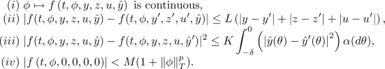
- (\(A_5\)):
-
The function f is non-anticipative.
- (\(A_6\)):
-
The function h is continuous and \( |h(\phi )|\le M(1+\left\| \phi \right\| _{T}^{p}),\) for all \(\phi \in {\Lambda }.\)
- (\(A_7\)):
-
The function \(\lambda \) is measurable and \( \lambda (z)\le M(1\wedge \vert z\vert )\), for all \(z \in {\mathbb {R}}_0.\)

The following remark generalizes a classical result, see, e.g., Theorem 14.1.1 in [15], Theorem 2.1 in [16] or Theorem 2.1 in [17].
Remark 1.5
In order to show both the existence and uniqueness of a solution to the backward part of the system (1.7) and to obtain the continuity of \(Y^{t,\phi }\) with respect to \(\phi \), we need to impose K or \(\delta \) to be small enough. More precisely, we will assume that there exists a constant \(\chi \in (0,1) \), such that:
The main difference between our result and Theorem 3.4 in [11] relies upon the presence of a jump component in the dynamics of the unknown process \(Y^{t,\phi }\): this further term implies a stronger bound in the condition enforced in Eq. (3.1).
Hence, if K or \(\delta \) are small enough to satisfy the condition stated in Eq. (3.1), then there exists a unique solution of (2.5) and the following theorem holds
Theorem 1.6
Let assumptions (\(A_1\))–(\(A_7\)) hold. If condition (3.1) is satisfied, then there exists a unique solution \((Y^{t,\phi }, Z^{t,\phi }, U^{t, \phi })_{(t, \phi )\in [0,T]\times \Lambda }\) of the BSDE (2.5) such that \((Y^{t,\phi }, Z^{t,\phi }, U^{t, \phi })\in {\mathbb {S}}_t^2 ({\mathbb {R}}) \times {\mathbb {H}}^2_t ({\mathbb {R}}^{ l}) \times {\mathbb {H}}_{t,\nu }^2 ({\mathbb {R}})\) for all \(t\in [0,T]\) and the application \(t \mapsto (Y^{t,\phi }, Z^{t,\phi }, U^{t, \phi })\) is continuous from [0, T] into \( {\mathbb {S}}_0^2 ({\mathbb {R}}) \times {\mathbb {H}}^2_0 ({\mathbb {R}}^{l}) \times {\mathbb {H}}_{0,\nu }^2 ({\mathbb {R}})\).
The proof of Theorem 3.3 is provided in “Appendix 7” and it is mainly based on the Banach fixed point theorem.
We emphasize that similar results hold also for multi-valued processes, namely \(Y: \Omega \times [0,T] \rightarrow {\mathbb {R}}^m\), \(Z: \Omega \times [0,T] \rightarrow {\mathbb {R}}^{m \times l}\) and \(U: \Omega \times [0,T] \times ({\mathbb {R}}^n {\setminus } \{0\}) \rightarrow {\mathbb {R}}^m\). Further difficulties may arise, due to the presence of correlation between the different components of \(Y \in {\mathbb {S}}_t^2 ({\mathbb {R}}^m)\) or the necessity of introducing the n-fold iterated stochastic integral, see [5, 7] or [12, Sec. 2.1] for further details.
4 The Feynman–Kac formula
In what follows we prove that the solution of Eq. (1.7), namely the path-dependent forward-backward system with delayed generator f and driven by a Lévy process, can be connected to the solution of path-dependent PIDE represented by the nonlinear Kolomogorov equation (1.1).
4.1 The Delfour–Mitter space
According to [2], we need the solution of the forward SDE (1.7) to be a Markov process to derive the Feynman–Kac formula. The Markov property of the solution is fully known for the SDE without jumps, i.e. when \(\gamma = 0\), see [29] (Th. III. 1.1). Moreover, the Markov property also holds, by enlarging the state space, for the solution in a setting analogous to that of Eq. (2.4), see [12] (Prop. 2.6) where driving noises with independent increments are considered. Since \(X^{t,\phi }: \Omega \times [0,T] \times D ([0,T]; {\mathbb {R}}^d) \rightarrow {\mathbb {R}}^d\) in not Markovian, we enlarge the state space by considering the process X as a process of the path, by introducing a suitable Hilbert space, as described in [22, 28], where they present a product-space reformulation of (2.4) splitting the present state X(t) from the past trajectory \(X_t\) by a particular choice of the state space. Accordingly, we enlarge the state space of our interest, starting from paths defined on the Skorohod space \(D \left( [0,T]; {\mathbb {R}}^d \right) \) to then consider a new functional space, the so-called Delfour–Mitter space \(M^2:= L^2 ([-T,0]; {\mathbb {R}}^d) \times {\mathbb {R}}^d \), by exploiting the continuous embedding of \(D\left( [-T,0]; {\mathbb {R}}^d \right) \) into \(L^2 ([-T,0]; {\mathbb {R}}^d)\), as in-depth analyzed in, e.g., [2, 12].
It is worth mentioning that \(M^2\) has a Hilbert space structure, endowed with the following scalar product
with associated norm
where \(\cdot \) and \(|\cdot |\) stand for the scalar product in \({\mathbb {R}}^d\), resp. for the Euclidean norm in \({\mathbb {R}}^d\), while \(\langle \cdot , \cdot \rangle _{L^2}\), resp. \(||\cdot ||_{L^2}\), indicates the scalar product, resp. the norm in \(L^2:= {L^2}([-T, 0];{\mathbb {R}}^d)\).
For \(t\in [0,T]\), \(\phi \in \Lambda \) and \((\varphi ,x)\in M^{2}\), let us set:
-
compatible initial conditions \( x^{t,\phi }:= \phi (t)\) and \(\eta ^{t,\phi }\in D([-T,0];{\mathbb {R}}^{d})\) defined by
 (4.1)
(4.1) -
\((\varphi ,x)^{t}\in \Lambda \) defined by
 (4.2)
(4.2) -
\({\tilde{b}}:[0,T]\times M^{2}\rightarrow {\mathbb {R}}^{d}\), \(\tilde{\sigma }:[0,T]\times M^{2}\rightarrow {\mathbb {R}}^{d\times l}\), \(\tilde{\gamma }:[0,T]\times M^{2}\times {\mathbb {R}}\rightarrow {\mathbb {R}}^{d}\) defined by
 (4.3)
(4.3)


where \(b:[0,T]\times \Lambda \rightarrow {\mathbb {R}}^{d}\), \(\sigma :[0,T]\times \Lambda \rightarrow {\mathbb {R}}^{d \times l}\) and \(\gamma :[0,T]\times \Lambda \times {\mathbb {R}}\rightarrow {\mathbb {R}}^{d}\) are the given coefficients of Eq. (2.4).
We emphasize that \((\varphi ,x)^{t}\) is well defined since it does not depend on the choice of the representative in the class of \(\varphi \in L^{2}\), and the continuous embedding \(D\left( [-T,0]; {\mathbb {R}}^d \right) \subset M^2\) is also injective.
We can now rewrite the forward equation (2.4) in the \(M^2\)-setting:

Here, for a process X, the term \(X_r\) means \((X((r + \theta )^+))_{\theta \in [-T, 0]}\), which is slightly different from the delayed term introduced in (1.8). Since this notation occurs only in the context of the \(M^2\)-setting for the forward equation, the reader can clearly distinguish between the two uses.
The link between the solution of equation Eq. (2.4) and that of equation Eq. (4.4) is then provided by
In order to take advantage of the Feynman–Kac formula already derived in [12] in the case of non-delayed but still path-dependent BSDE, we have to additionally impose that b, \(\sigma \), \(\gamma \), f and h are locally Lipschitz-continuous with respect to \(\phi \in \Lambda \) in the \(L^{2}\)-norm. Thus, in order to have the same regularity for the solution of the BSDE system with forward Eq. (4.4), we require that the coefficients b, \(\sigma \) and \(\gamma \) to be locally Lipschitz.
Assumption 1.7
There exists \(K \ge 0\) and \(m \ge 0\) such that:
- (\(A_8\)):
-
for all \(t \in [0,T]\) and for all \(\phi _1, \phi _2 \in \Lambda \),
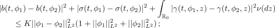
- (\(A_9\)):
-
for all \(t \in [0,T]\), \(y \in {\mathbb {R}}\), \(z \in {\mathbb {R}}^l\), \(u \in {\mathbb {R}}\), \({\hat{y}} \in L^2 ([-\delta ,0]; {\mathbb {R}})\) and for all \(\phi _1, \phi _2 \in \Lambda \),

- (\(A_{10}\)):
-
for all \(\phi _1, \phi _2 \in \Lambda \),
$$\begin{aligned} |h (\phi _1) - h(\phi _2)| \le K (1 + ||\phi _1||_{L^2} + ||\phi _2||_{L^2} )^m || \phi _1 - \phi _2||_{L^2} \,. \end{aligned}$$


We remark that \({\tilde{b}}\), \({\tilde{\sigma }}\) and \({\tilde{\gamma }}\), as defined by (4.3) are not necessarily locally Lipschitz, since \(D \left( [0,T]; {\mathbb {R}}^d \right) \) is dense in \(L^2\left( [0,T]; {\mathbb {R}}^d \right) \), but they are set to constants outside \(D \left( [0,T]; {\mathbb {R}}^d \right) \). However, one can define these coefficients first on \([0,T]\times D \left( [0,T]; {\mathbb {R}}^d \right) \times {\mathbb {R}}^d\) and then extend to \([0,T]\times M^2\) by density, using the uniform continuity provided by assumption \((A_8)\). It is this version of the above functions that we will use in the sequel.
Within this setting, lifting the state space turns out to be particularly convenient in order to investigate differentiability properties of the solution and relate the solution of Eq. (4.4) (combined with the backward equation) to the solutions of the non-linear Kolmogorov equation defined by Eq. (1.1) on \([0,T] \times \Lambda \).
Remark 1.8
It is also possible to work directly on the Skorohod space D. However, since D is not a separable Banach space, one has to consider weaker topologies on D, following a semi-group approach like the one developed by Peszat and Zabczyk in [36].
4.2 Main theorem
In what follows we provide the main result, namely a nonlinear version of the Feynman–Kac formula in the case where the process \(X^{t,\phi }\) has jumps and the generator of the backward dynamic f depends on the past values of Y.
Theorem 1.9
(Feynman–Kac formula) Under hypotheses (\(A_1\))–(\(A_{10}\)) with condition (3.1) being verified, let \((X^{t, \phi }, Y^{t, \phi }, Z^{t, \phi }, U^{t, \phi })_{(t, \phi )\in [0,T]\times \Lambda }\) be the solution of the forward-backward system (2.3).
Let \(u: [0,T] \times \Lambda \rightarrow {\mathbb {R}}\) be the deterministic function defined by
Then u is a non-anticipative function and there exist constants \(C>0\) and \(m\ge 0\) such that, for all \(t\in [0,T]\) and \(\phi _1,\phi _2\in \Lambda \),
Moreover, the following formula holds:
for any \((t,\phi ) \in [0,T] \times \Lambda \).
To prove the representation formula (4.6), we adapt the proof of Theorem 4.10 of [11] by adding the contribution of U and \({\tilde{U}}\), respectively modelling the process and the integral term connected to the jump component.
Proof
We follow the Picard iteration scheme, hence considering the iterative process of the BSDE with a delayed generator driven by Lévy process described by

with \(Y^{0,t,\phi } \equiv 0 \), \(Z^{0,t,\phi } \equiv 0 \) and \(U^{0,t,\phi } \equiv 0 \) and initial condition
Let us suppose that there exists a non-anticipative functional \(u_n: [0,T] \times \Lambda \rightarrow {\mathbb {R}}\) such that \(u_n\) is locally Lipschitz and \(Y^{n, t, \phi } (s) = u_n (s, X^{t, \phi })\) for every \(t,s \in [0,T]\) and \(\phi \in \Lambda \).
Since \(Y^{n, t, \phi } (r + \theta ) = u_n (r + \theta , X^{t, \phi } )\) if \(r+\theta \ge 0\) and \(Y^{n, t, \phi } (r + \theta ) = Y^{n, t, \phi } (0) = u_n (0, X^{t, \phi })\) if \(r + \theta < 0\), by defining
the delayed term reads
and the above equation becomes

For fixed n, we define \(\psi _n:[0,T]\times D([-T,0];{\mathbb {R}}^{d})\times {\mathbb {R}}^{d}\times {\mathbb {R}}\times {\mathbb {R}}^{l }\times {\mathbb {R}} \rightarrow {\mathbb {R}}\) as
and \({\tilde{h}}:D([-T,0];{\mathbb {R}}^{d})\times {\mathbb {R}}^{d}\rightarrow {\mathbb {R}}\) as
Since \(u_{n}\) is locally Lipschitz-continuous, one can show that \(\psi _n\) and \({\tilde{h}}\) are also locally Lipschitz in \(\varphi \). Therefore, one can extend them by density to \([0,T]\times M^2\times {\mathbb {R}}\times {\mathbb {R}}^{l }\times {\mathbb {R}}\), respectively to \(M^2\), keeping the locally Lipschitz property.
After setting \(\eta =\eta ^{t,\phi }\), \(x=x^{t,\phi }\) (see (4.1)), we enlarge the state space and write the forward–backward system in an equivalent way as (for simplicity, we omit the dependence of n)

It is easy to see that the two sets of solutions, \(\left( X^{t,\eta ,x},Y^{t,\eta ,x},Z^{t,\eta ,x}, U^{t,\eta ,x}\right) \) and \(\left( X^{t,\phi },Y^{n+1,t,\phi },Z^{n+1,t,\phi }, U^{n+1,t,\phi }\right) \) coincide.
We have already observed that the extended coefficients \({\tilde{b}}\), \({\tilde{\sigma }}\), \({\tilde{\gamma }}\) satisfy conditions (A1)–(A2) in [12, pp. 8–9]; in a similar manner, \(\psi _n\) and \({\tilde{h}}\) satisfy (B1) and (B2) in [12, p. 24]. Then we can exploit Theorem 4.5 in [12] and infer that there exists a locally Lipschitz function \({\bar{u}}_n:[0,T]\times M^{2} \rightarrow {\mathbb {R}}\) such that the following representation formula holds:
Let us define the following locally Lipschitz, non-anticipative functional \(u_{n+1}:[0,T]\times \Lambda \rightarrow {\mathbb {R}}\) by
where the time shifting \(\eta ^{t,\phi }\) is defined according to (4.1). Then
Notice that \(\left( Y^{n,t, \phi }, Z^{n,t, \phi }, U^{n,t, \phi } \right) \) is the Picard iterative sequence needed to construct the solution \(\left( Y^{t, \phi }, Z^{t, \phi }, U^{t, \phi } \right) \):
where \(\Gamma \) is the contraction defined in the proof of Theorem 3.3. By applying Theorem 3.3, we then have:
Of course, \(u_{n}(t,\phi )\) converges to \(u(t,\phi ):={\mathbb {E}} \, [ Y^{t,\phi }(t)],\) for every \(t\in [0,T]\) and \(\phi \in {\Lambda }\), hence implying that the nonlinear Feynman–Kac formula \(Y^{t,\phi }\left( s\right) =u(s,X^{t,\phi })\) holds. From its definition, it is clear that u is non-anticipative. Regarding the locally Lipschitz property, it can be proven by applying Itô’s formula to \(|Y^{t,\phi _1}-Y^{t,\phi _2}|^2\) and resorting to standard calculus. \(\square \)
5 Mild solution of the Kolmogorov equation
In this section, we prove the existence of a mild solution of the path-dependent partial integro-differential equation (PPIDE) Kolmorogov equation (1.1) showing a dependence both on a delayed term and on integral term modelling jumps.
Let us start by recalling from [12] the notion of the Markov transition semigroup corresponding to the operator \({\mathcal {L}}\) introduced by (1.4). From [12, Prop. 2.6], we know that the strong solution \(X^{0,\eta ,x} \in M^2\) of Eq. (4.4) is a Markov process in the sense that \({\mathbb {P}}\)-a.s.,
for all \((\eta ,x)\in M^2\) and all Borel sets B of \(M^2\), the proof of this fundamental result being given in several works, as, e.g. [2, Th. 3.9], [37, Prop. 3.3] or [36, Sec. 9.6]; for more details, see, e.g., [23].
Denoting by \(B_p(S)\) the space of Borel functions with at most polynomial growth on a metric space S, the transition semigroup \({\tilde{P}}_{t,s}\), acting on \(B_p(M^2)\) is then defined by
Coming back to our setting, we define \({P}_{t,s}:B_p(\Lambda )\rightarrow B_p(\Lambda )\) by
Obviously (see (4.1) for the notations), for \(\varphi \in B_p(\Lambda )\) and \(\phi \in \Lambda ,\)
In order to introduce the notion of mild solution, we will need to define the generalized directional gradient of a function \(u:[0,T]\times \Lambda \rightarrow {\mathbb {R}}\), following the approach in [23], also described in [12]. Suppose that the function u satisfies the following locally Lipschitz-continuity condition:
Since the procedure of defining the generalized directional gradient takes place in Hilbert spaces, we will have to appeal again to the \(M^2\)-lifting, as we have already done for the coefficients of the forward equation. We define first
for \((t,\varphi ,x)\in [0,T]\times D([-T,0];{\mathbb {R}}^{d})\times {\mathbb {R}}^{d}\) and then extend it to \([0,T]\times M^2\) by density. Again, this is possible due to condition (5.2). Then, according to [23, Th. 3.1], there exists a Borel function \(\zeta :[0,T]\times M^2\rightarrow {\mathbb {R}}^d\) such that
for any \(0\le t\le \tau \le T\) and \((\eta ,x)\in M^2\), where \(\langle X,Y\rangle _{[t,\tau ]}\) denotes the joint quadratic variation of a pair of real stochastic processes \((X(t),Y(t))_{t\in [0,T]}\) on the interval \([t,\tau ]\),
with the limit taken in probability and X(s), Y(s) defined as X(s), respectively Y(s) for \(s>T\).
The set of all functions \(\zeta \) with the above property is called the generalized directional gradient of v and is denoted \(\nabla ^{\sigma } v\). Its name and notation come from the observation that if v (and, consequently u) and the coefficients of the forward equation are sufficiently regular, then \(\nabla _{(\eta ,x)} v\cdot {\tilde{\sigma }}\in \nabla ^{\sigma } v\) (see [23, Remark 3.3]).
We come back to the \(\Lambda \)-setting and define \(\nabla ^{\sigma } u\), the generalized directional gradient of u as the set of all non-anticipative functions \(\xi :[0,T]\times \Lambda \rightarrow {\mathbb {R}}\) such that there exists \(\zeta \in \nabla ^{\sigma }v\) satisfying
for all \((t,\varphi ,x)\in [0,T]\times D([-T,0];{\mathbb {R}}^{d})\times {\mathbb {R}}^{d}\). Such a function can be defined by setting \(\xi (t,\phi ):=\zeta (t,\eta ^{t,\phi },x^{t,\phi })\).
It is clear that relation (5.3) translates into
for all \((t,\phi )\in [0,T]\times \Lambda \) and all \(\tau \in [t,T]\), if \(\xi \in \nabla ^{\sigma }u\). From this relation, it is clear (see also Remark 3.2 in [23]) that if \(\xi ,{\hat{\xi \in \nabla }}^{\sigma }u\), then
so there is no ambiguity if we write \(\nabla ^{\sigma } u(s,X^{t,\phi })\).
We have now all the ingredients for introducing the notion of a mild solution.
Definition 1.10
A non-anticipative function \(u:[0,T] \times \Lambda \rightarrow {\mathbb {R}}\) is a mild solution to Eq. (1.1) if u satisfies (5.2) and the following equality holds true for all \((t,\phi ) \in [0,T]\times \Lambda \) and \(\xi \in \nabla ^{\sigma } u\):
where \((u(\cdot , \cdot ))_s\) is the delayed term defined in (1.5).
Given the definition of \(P_{t,T}\) and the above mentioned remark, we can reformulate relation (5.4) as
The next theorem represents the core result of this section.
Theorem 1.11
(Existence and uniqueness) Let assumptions (\(A_1\))–(\(A_{10}\)) and (3.1) hold true. Then the function u defined by (4.6) is the unique mild solution to the path-dependent partial integro-differential Eq. (1.1).
Proof
Existence. Let us consider the backward component of the FBSDE described in Eq. (2.3) for \(s \in [t,T]\)
By Theorem 4.3, the non-anticipative function u defined by (4.6) is satisfying (5.2) (the second part comes the continuity of \(t\mapsto Y^{t,\phi }\), asserted in Theorem 3.3) and the representation formula (4.7) holds. Moreover, by means of Eq. (4.6), we can write the delayed term \(Y_r\) as a function of the path of solution of the forward dynamic \(X^{t, \phi }\) and, thus, by defining
we can rewrite Eq. (5.6), leading to

At this point, we enlarge the state space going through \(M^2\) coefficients analogously to the proof of Theorem 3.3, obtaining

where the map \({\tilde{h}}\) was defined in Eq. (4.9) and \(\psi \) is defined similarly to \(\psi _n\) introduced in Eq. (4.8):
on \([0,T]\times D([-T,0];{\mathbb {R}}^{d})\times {\mathbb {R}}^{d}\times {\mathbb {R}}\times {\mathbb {R}}^{l }\times {\mathbb {R}}\) and extending it by density. Since \({\tilde{h}}\) and \(\psi \) are locally Lipschitz, hence satisfying the conditions required by Theorem 4.8 in [12], we can apply this result in order to conclude that the function \(v:[0,T]\times M^2\rightarrow {\mathbb {R}}\) defined by
is a mild solution (in the sense of [12], but similar to ours) of the following PPIDE

where \(\tilde{{\mathcal {L}}}\) and \(\tilde{{\mathcal {J}}}\) are the straightforward modifications of \({\mathcal {L}}\), respectively \({\mathcal {J}}\) in \(M^2\). Since \(v (t, \phi , x)=u(t,(\varphi ,x)^{t})\) for any \((t,\phi , x)\in [0,T]\times D([-T,0];{\mathbb {R}}^{d})\), by playing on the relation (5.1) and the connection between the formulations of the generalized directional gradient in the càdlàg, respectively \(M^2\) cases, it is straightforward to show that u is a mild solution of (1.1).
Uniqueness. Let us take two mild solutions \(u^{1}\) and \(u^{2}\) of the path-dependent PDE (1.1). We define
Using these drivers we can consider the following BSDEs:
for which there exist unique solutions \(\left( Y^{i,t,\phi }\,, \, Z^{i,t,\phi } \,, U^{i,t,\phi } \, \right) \in {\mathbb {S}}_t^2 ({\mathbb {R}}) \times {\mathbb {H}}^2_t ({\mathbb {R}}^{l})\times {\mathbb {H}}_{t,\nu }^2 ({\mathbb {R}}) \) for \( i=\overline{1,2}\,.\)
By Theorem 4.3 we see that
for any \(\left( t,\phi \right) \in \left[ 0,T\right] \times \Lambda ,\) where \(v^{i}:\left[ 0,T\right] \times \Lambda \rightarrow {\mathbb {R}}\), \( i=\overline{1,2}\) are defined by
Hence, by the existence part, we obtain that the functions \(v^{i}\) are solutions of the PDE of type (1.1), but without the delayed terms \(\left( v^{i}\left( \cdot ,\phi \right) \right) _{t}:\)

Since \(u^{i}\) is also solution to equation (5.10), by using the uniqueness part of Theorem 4.5 from [12] we get that (after embedding these equations in \(M^2\), as we did in the previous part)
Hence
so BSDEs (5.9) become a single equation,
with \(i=\overline{1,2},\) for which we have uniqueness from Theorem 3.3.
Therefore \(Y^{1,t,\phi }=Y^{2,t,\phi }\) and, consequently
\(\square \)
Remark 1.12
From Theorem 4.5 in [12], besides relation (4.7), it can also be inferred that for every \((t,\phi )\in [0,T]\times \Lambda \) the following representation formulas hold, \({\mathbb {P}}\)-a.s. and for a.e. \(s \in [t,T]\):
where we use the notation introduced in (1.3). These formulas could have been used to prove directly the existence part of the above result, by taking the expectation in equation (5.7) and using relation (5.5).
6 Financial application
In this section, we provide a financial application moving from the model studied in, e.g. [13], or [19]. We consider a generalization of the so-called Large Investor Problem, where a large investor wishes to invest in a given market, buying or selling a stock. The investor has the peculiarity that his actions on the market can affect the stock price. We refer to Example 14.1 in [15] for a detailed example of the time-delayed setting for the large investor problem.
6.1 A perfect replication problem for a large investor
Concerning the problem of the perfect replication strategy for a large investor, we generalize Example 14.1 in [15] by asking, in addition to path-dependent coefficients, the dynamic of the risky asset driven by a Poisson random measure. Similar results are also presented in [11, 19].
We denote the investor’s strategy by \(\pi \) and the investment portfolio by \(X^\pi \) and we assume that its past \(X^\pi _r\) may affect directly the stock coefficients \(\mu \), \(\sigma \) and \(\gamma \) and the bond rate. Consequently, we consider the following dynamic

where \(r_i\), \(\mu _i\), \(\sigma _i\) and \(\gamma _i\), \(i=\overline{1,2}\) are \({\mathbb {F}}^{W, {\tilde{N}}}\)-predictable processes, \({\mathbb {F}}^{W, {\tilde{N}}}\) being the natural filtration associated to the Brownian motion W and to the Poisson random measure \({\tilde{N}}\), with compensator defined according to Eq. (2.1).
The total amount of the portfolio of the large investor is described by

where, at any time \(t\in [0,T],\) \( \pi _i (t)\) represents the amount invested in the risky asset \(S_i\), while \(X^\pi (t)- \pi _1(t)-\pi _2(t)\) is the amount invested in the riskless one \(S_0\).
Let us denote, for simplicity, \(\phi :=(\phi _1,\phi _2)\) for \(\phi \) among the symbols S, \(\pi \), \(\mu \), \(\sigma \) or \(\gamma \) and by \(\cdot \) the scalar product in \({\mathbb {R}}^2\). The goal is to find an admissible replicating strategy \(\pi \in {\mathcal {A}}\) for a claim h(S(T)).
We have that the portfolio X evolves according to

Hence, for \(t\in \left[ 0,T\right] \), we have
with final condition \(X^\pi (T)=h\left( S\right) \) by denoting
The generator F can be rewritten to accommodate the dependence of \(Z^\pi \) and \(U^\pi \) by introducing the following transformation
since from Eq. (6.3) we have
by imposing that the matrix \(\begin{bmatrix} \sigma ^\mathrm{{T}}&\gamma ^\mathrm{{T}} \end{bmatrix}\) is invertible.
We then ask the coefficients \(r,\mu \), \(\sigma \) and \(\gamma \) to be such that the function \({\bar{F}}: [0,T] \times {\mathbb {R}} \times L^2 \left( [-\delta , 0]; {\mathbb {R}}\right) \times {\mathbb {R}}\times {\mathbb {R}} \rightarrow {\mathbb {R}}\) satisfies assumptions \((A_{4})\), \((A_{5})\) and \((A_{9})\).
Furthermore, we need a couple of simplifying assumptions in order to fit the theoretical framework of the article.
First, we introduce a functional aiming at encoding the forward process in order to decouple the terminal condition in the BSDE (6.2) from the stock forward dynamic (6.1). The risky assets vector S can be explicitly written, by a variation of constants formula, as a functional of the random coefficients of the stock (W and \({\tilde{N}}\)), on the wealth X and on the processes Z and U depending on the allocation strategy \(\pi \). Hence h(S(T)) can be written as
where \({\bar{h}}\) is asked to satisfy, besides conditions \((A_6)\) and \((A_{10})\) in the first two coefficients, a Lipschitz condition in the last three with Lipschitz constant \(K_1\).
Thus, we can rewrite (6.2) as

If we assume that \(\delta = T\) and the Lipschitz constants K and \(K_1\) are sufficiently small, then the time-delayed BSDE (6.6) has a unique solution. The setting is a little more general than ours, in the sense that the final condition also depends on the path of the solution of the backward equation (6.6), but one can use Theorem 14.1.1 in [15].
The further modelling concerns introducing the Markovian setting, i.e. allowing the initial time and value to vary. Hence, we introduce the forward processes \({\bar{W}}\) and \({\bar{N}}\) by

with Brownian motion W, compensated Random measure \({\tilde{N}}\) and an initial càdlàg datum \(\phi =(\phi _{1},\phi _{2}) \in \Lambda \).
Finally, by recalling the coefficients \({\bar{F}}\), Z and U defined in Eq. (6.3) we may write the following decoupled forward–backward stochastic system:
where the BSDE coefficients are defined according to (6.3).
Then, imposing the same assumptions as before (where \(t=0\)) there exists a unique solution \(\left( X^{t,\phi },Z^{t,\phi },U^{t,\phi }\right) _{\left( t,\phi \right) \in \left[ 0,T\right] \times {\Lambda }}\) for the BSDE in (6.8). Again, the final condition is a little more general that we have in our theoretical framework, but this can be easily modified by adapting the proof of Theorem 3.3, as it is done, for example in Theorem 14.1.1 in [15].
Moreover, by Theorem 4.3, the solution of the backward equation in the above system can be expressed as
for every \(\left( t,\phi \right) \in \left[ 0,T\right] \times { \Lambda },\) where \(u\left( t,\phi \right) :=X^{t,\phi }\left( t\right) \). Furthermore, u is the mild solution, according to Definition 5.1, of the following path-dependent PDE:

with \((t,\phi ) \in [0,T)\times \Lambda \).
We also present a concrete example of a jump-diffusion model for option pricing that can help the reader to link the forward dynamic to a tractable application. This example has a clear limitation if applied to our setting, such as no path-dependence in the coefficients of the stock dynamic (6.9) but only in the terminal condition h of the BSDE. Moreover, if we need to assume suitable conditions on \(\mu \), \(\sigma \) and \(\gamma \), e.g. asking \(\mu \) bounded and \(\sigma \), \(\gamma \) constant (w.r.t. X), so that the terminal condition also satisfies the required Lipschitz condition.
Example 6.1
(Forward SDE with a discrete number of jumps). The stock price may present a jump–diffusion dynamic with a discrete number of jumps triggered by a Poisson process, namely we consider the following equation
in place of Eq. (6.1), where N(t) is a standard Poisson process of fixed rate and jumps size \(\{ V_i\}\) modelled as a sequence of independent, identically, distributed non-negative random variables. We consider independence among all the sources of randomness, namely W and N. We refer to, e.g., [26] for a detailed treatment of this kind of jump-diffusion. Firstly, we notice that the forward Eq. (6.9) can be explicitly solved by the following
If we assume no path-dependence in the coefficients, such as in Eq. (6.9), then we may encode in the terminal condition of the BSDE (6.2), a dependence only on W, N and \(\{ V_i\}\). Hence, by introducing the following functional
we can decouple the FBSDEs system to fit the setting of Theorem 3.3.
7 Conclusions and future development
The core result of this paper relies on deriving a stochastic representation for the solutions of a non-linear PDE and associating the PDE solution to a FBSDE with jumps and a time-delayed generator. The presence of jumps both in the forward and backward dynamic and, moreover, the dependence of the generator on a (small) time-delayed coefficient represents the main aspect of novelty arising in the analysis of this kind of FBSDE system. Furthermore, we present an application for a large investor problem admitting a jump–diffusion dynamic. Throughout the article, we mention some possibilities to generalize the setting of our equations such as considering the dependence of f also on a delayed term for the processes Z and U, see Remark 2.1 for more details, or in-depth analyzing the choice of a weaker topology, see Remark 4.2. A different modelling choice deals with considering a further delay term affecting the forward process, see [27] for more details. Furthermore, it might deserve attention to investigate a discretization scheme for this equation, e.g. in line with [7], for the considered equations to obtain a numerical approach based on Neural Networks methods to efficiently compute an approximated solution for the considered FBSDE.
References
Applebaum, D.: Lèvy Processes and Stochastic Calculus. University Press, Cambridge (2000)
Baños, D.R., Cordoni, F., Di Nunno, G., Di Persio, L., Røse, E.E.: Stochastic systems with memory and jumps. J. Differ. Equ. 266(9), 5772–5820 (2019)
Barles, G., Buckdahn, R., Pardoux, E.: Backward stochastic differential equations and integral-partial differential equations. Stoch. Stoch. Rep. 60, 57–83 (1997)
Bass, R.F.: Stochastic differential equations with jumps. Probab. Surv. 1, 1–19 (2005)
Bell, D.R., Mohammed, S.E.A.: The Malliavin calculus and stochastic delay equations. J. Funct. Anal. 99(1), 75–99 (1991)
Bichteler, K.: Stochastic Integration with Jumps Encyclopedia of Mathematics and its Applications. Cambridge University Press, Cambridge (2002). https://doi.org/10.1017/CBO9780511549878
Bouchard, B., Elie, R.: Discrete-time approximation of decoupled forward–backward SDE with Jumps. Stoch. Process. Appl. 118, 53–75 (2008)
Cont, R.: Functional Ito calculus and functional Kolmogorov equations (2020)
Cont, R., Fournié, D.A.: Change of variable formulas for non-anticipative functionals on path space. J. Funct. Anal. 259(4), 1043–1072 (2010)
Cont, R., Fournié, D.A.: Functional Itô calculus and stochastic integral representation of martingales. Ann. Probab. 41(1), 109–133 (2013)
Cordoni, F., Di Persio, L., Maticiuc, L., Zălinescu, A.: A stochastic approach to path-dependent nonlinear Kolmogorov equations via BSDEs with time-delayed generators and applications to finance. Stoch. Process. Appl. 130(3), 1669–1712 (2020)
Cordoni, F., Di Persio, L., Oliva, I.: A nonlinear Kolmogorov equation for stochastic functional delay differential equations with jumps. Nonlinear Differ. Equ. Appl. 24, 16 (2017)
Cvitanic, J., Ma, J.: Hedging options for a large investor and forward-backward SDEs. Ann. Appl. Probab. 6(2), 370–398 (1996)
Delong, Ł.: Applications of time-delayed backward stochastic differential equations to pricing, hedging and portfolio management. arXiv e-prints (2010)
Delong, Ł: Backward Stochastic Differential Equations with Jumps and Their Actuarial and Financial Applications: BSDEs with Jumps. EAA Series, Springer, London (2013)
Delong, Ł, Imkeller, P.: Backward stochastic differential equations with time delayed generators—results and counterexamples. Ann. Appl. Probab. 20(4), 1512–1536 (2010)
Delong, Ł, Imkeller, P.: On Malliavin’s differentiability of BSDEs with time delayed generators driven by Brownian motions and Poisson random measures. Stoch. Process. Appl. 120(9), 1748–1775 (2010)
Dupire, B.: Functional Itô Calculus. Portfolio Research Paper, Bloomberg (2010)
El Karoui N., Peng S., Quenez M.C.: A dynamic maximum principle for the optimization of recursive utilities under constraints. Ann. Appl. Probab. 664–693 (2001)
Ekren, I., Keller, C., Touzi, N., Zhang, J.: Viscosity solutions of fully nonlinear parabolic path dependent PDEs: part I. arXiv:1210.0006v3 (2014)
Ekren, I., Keller, C., Touzi, N., Zhang, J.: Viscosity solutions of fully nonlinear parabolic path dependent PDEs: part II. arXiv: 1210.0007v3 (2014)
Flandoli, F., Zanco, G.: An infinite-dimensional approach to path-dependent Kolmogorov’s equations. Ann. Probab. 44(4), 2643–2693 (2016)
Fuhrman, M., Tessitore, G.: Generalized directional gradients, backward stochastic differential equations and mild solutions of semilinear parabolic equations. Appl. Math. Optim. 51, 279–332 (2005)
Fuhrman, M., Tessitore, G.: Nonlinear Kolmogorov equations in infinite dimensional spaces: the backward stochastic differential equations approach and applications to optimal control. Ann. Probab. 30(3), 1397–1465 (2002)
Kac, M.: On some connections between probability theory and differential and integral equations (1951)
Kou, S.G.: A jump-diffusion model for option pricing. Manag. Sci. 48(8), 1086–1101 (2002)
Ma, T., Xu, J., Zhang, H.: Explicit solution to forward and backward stochastic differential equations with state delay and its application to optimal control. Control Theory Technol. 20, 303–315 (2022)
Masiero, F., Orrieri, C., Tessitore, G., Zanco, G.: Semilinear Kolmogorov equations on the space of continuous functions via BSDEs. Stoch. Process. Appl. 136, 1–56 (2021)
Mohammed, S.E.A.: Stochastic Functional Differential Equations, Research Notes in Mathematics, vol. 99. Pitman (Advanced Publishing Program), Boston (1984)
Mohammed, S.E.A.: Stochastic differential systems with memory: theory, examples and applications (1998)
Pardoux, E., Peng, S.: Adapted solution of a backward stochastic differential equation. Syst. Control Lett. 14, 55–61 (1990)
Pardoux, E., Peng, S.: Backward SDEs and quasilinear PDEs. In: Rozovskii, B.L., Sowers, R. (eds.) Stochastic Partial Differential Equations and Their Applications. LNCIS, vol. 176. Springer, New York (1992)
Pardoux, E., Pradeilles, F., Rao, Z.: Probabilistic interpretation of a system of semi-linear parabolic partial differential equations. Annales de l’I.H.P. Probabilités et statistiques, Tome 33(4), 467–490 (1997)
Peng, S.: Backward stochastic differential equation, nonlinear expectation and their applications. In: Proceedings of the International Congress of Mathematicians Hyderabad, India (2010)
Peng, S., Wang, F.: BSDE, path-dependent PDE and nonlinear Feynman–Kac formula. Sci. China Math. 59, 19–36 (2016)
Peszat, S., Zabczyk, J.: Stochastic Partial Differential Equations with Lévy Noise: An Evolution Equation Approach, Encyclopedia of Mathematics and its Applications. Cambridge University Press, Cambridge (2007)
Reib, M., Riedle, M., van Gaans, O.: Delay differential equations driven by Lévy processes: stationarity and Feller properties. Stochastic Processes and their Applications 116(10), 1409–1432 (2006)
Skorokhod, A.V.: Studies in the Theory of Random Processes. Inc., Addison-Wesley Publishing Co. Inc, Reading, Translated from the Russian by Scripta Technica (1965)
Yan, F., Mohammed, S.E.A.: A stochastic calculus for systems with memory. Stoch. Anal. Appl. 23(3), 613–657 (2005)
Funding
Open access funding provided by Università degli Studi di Trento within the CRUI-CARE Agreement. No funds, grants, or other support was received.
Author information
Authors and Affiliations
Contributions
All authors contributed to the study conception and design. All authors read and approved the final manuscript.
Corresponding author
Ethics declarations
Conflict of interest
The authors declare they have no financial interests.
Additional information
Publisher's Note
Springer Nature remains neutral with regard to jurisdictional claims in published maps and institutional affiliations.
Proof of Theorem 3.3
Proof of Theorem 3.3
Proof
The existence and the uniqueness are obtained by the Banach fixed point theorem. We consider \(\phi \) fixed in \(\Lambda \) and we define the map \(\Gamma \) on \({\mathcal {A}}\) with \({\mathcal {A}}:= {\mathcal {C}} \big ( [0,T] \,; \, {\mathbb {S}}_0^2 ({\mathbb {R}}) \big )\).
For \(R \in {\mathcal {A}}\), we define \(\Gamma (R): = Y\), where, for \(t \in [0,T]\), the triple of adapted processes \(\big ( Y^t (s),Z^t(s),U^t (s,z) \big )_{s \in [t,T]}\) is the unique solution of the following BSDE
For \(s \in [0,t]\) we prolong the solution by taking \(Y^t (s):= Y^s (s)\) and \(Z^t (s) = U^{t,\phi } (s):= 0\).
Step 1. Let us first show that \(\Gamma \) takes values in the Banach spaces \({\mathcal {A}}\). We take \(R \in {\mathcal {A}}\) and we will prove that \(Y:= \Gamma (R) \in {\mathcal {A}}\). Thus, for every \(t \in [0,T]\) we have to show that
and that the application
is continuous.
Let \(t\in \left[ 0,T\right] \) be fixed and \(t^{\prime }\in [0,T]\); with no loss of generality, we will suppose that \(t<t^{\prime }\) and \(t^{\prime }-t<\delta \).
Concerning the solution of the BSDE defined in (A.1), we obtain the following estimate

We start by proving that
as \(t^{\prime }\rightarrow t\). By plugging the explicit solution and applying Doob’s inequality, we get
From the absolute continuity of the Lebesgue integral, we deduce that
as \(t^{\prime }\rightarrow t\).
Concerning the term \({\mathbb {E}}\big (\sup _{s\in \left[ t^{\prime },T\right] }|Y^{t}\left( s\right) -Y^{t^{\prime }}\left( s\right) |^{2}\big )\) let us denote for short, only throughout this step,
and
We apply Itô’s formula to \(e^{\beta s}|\Delta Y\left( s\right) |^{2}\) and we derive, for any \(\beta >0\) and any \(s\in \left[ t^{\prime },T\right] ,\)
We note that the following estimate
holds. From assumptions \((A_3)\)–\((A_5)\), we have for any \(a>0,\)
Therefore we have
We now choose \(\beta ,a>0\) such that
hence we obtain
By Burkholder–Davis–Gundy’s inequality, we have
and
which immediately implies
Hence, we have
where
Exploiting thus assumptions \((A_3)\) and \((A_5)\) together with the fact that \(X^{\cdot ,\phi }\) is continuous and bounded, we have
Since \( R \in {\mathcal {A}} \), and therefore we have
as \(t^{\prime }\rightarrow t\), we have
as \(t^{\prime }\rightarrow t\).
We are left to show that the term \({\mathbb {E}}\big (\sup _{s\in \left[ t,t^{\prime }\right] }|Y^{t}\left( t\right) -Y^{s}\left( s\right) |^{2}\big )\) is also converging to 0 as \(t^{\prime }\rightarrow t\).
Since the map \(t\mapsto Y^{t}\left( t\right) \) is deterministic, we have from equation (A.1),
Using then the assumption (A\(_{3}\)) we have
and therefore we obtain
Taking again into account the fact that \( R \in {\mathcal {A}}\), previous step and assumptions \((A_3)\) and \((A_5)\), we infer that
Concerning the term \({\mathbb {E}}\int _{0}^{T}|Z^{t}\left( r\right) -Z^{t^{\prime }}\left( r\right) |^{2}dr\), we see that
hence, by (A.3),
Analogously, we can infer that
as \( t^{\prime } \rightarrow t\).
Step II. Step 2. We are going to prove that \(\Gamma \) is a contraction on \({\mathcal {A}}\) with respect to the norm
Let us recall that \(\Gamma :{\mathcal {A}}\rightarrow \mathcal {A }\) is defined by \(\Gamma \left( R \right) = Y \) being Y the process coming from the solution of the BSDE (A.1).
Let us consider \( R^{1}, R^{2} \in {\mathcal {A}}\) and \( Y^{1}:=\Gamma \left( R^{1}\right) \), \(Y^{2}:=\Gamma \left( R^{2}\right) \). For the sake of brevity, we will denote in what follows
Proceeding as in Step I, we have from Itô’s formula, for any \(s\in \left[ t,T\right] \) and \(\beta >0\),
Noticing that it holds
we immediately have, from assumptions \((A_4)\)–\((A_6)\), that for any \(a>0\),
Therefore equation (A.8) yields
Let now \(\beta ,a>0\) satisfying
we have
Exploiting now Burkholder–Davis–Gundy’s inequality, we have
and, analogously,
which implies
Hence, we have
where we have denoted by \(C_{1}:=1+\frac{144}{1-4L^{2}/a}.\)
Let us now consider the term \({\mathbb {E}}\big (\sup _{s\in \left[ 0,t\right] }e^{\beta s}|\Delta Y\left( s\right) |^{2}\big )\). From equation (A.1), we see that,
so that, exploiting Itô’s formula and proceeding as above, we obtain
Thus from inequalities (A.12–A.15) we obtain
Then, passing to the supremum for \(t\in \left[ 0,T\right] \) we get
By choosing now \(a:=\frac{4\,L^{2}}{\chi }\) and \(\beta \) slightly bigger than \(\chi +\frac{4L^{2}}{\chi }\), condition (A.11) is satisfied and, by restriction \(\mathrm {(C)}\) we have
Eventually, since R is chosen arbitrarily, it follows that the application \(\Gamma \) is a contraction on \({\mathcal {A}}\). Therefore, there exists a unique fixed point \(\Gamma (R)=Y \in {\mathcal {A}}\) and this finishes the proof of the existence and uniqueness of a solution to BSDE with delay and driven by Lèvy process, described by Eq. (2.5).\(\square \)
Rights and permissions
Open Access This article is licensed under a Creative Commons Attribution 4.0 International License, which permits use, sharing, adaptation, distribution and reproduction in any medium or format, as long as you give appropriate credit to the original author(s) and the source, provide a link to the Creative Commons licence, and indicate if changes were made. The images or other third party material in this article are included in the article’s Creative Commons licence, unless indicated otherwise in a credit line to the material. If material is not included in the article’s Creative Commons licence and your intended use is not permitted by statutory regulation or exceeds the permitted use, you will need to obtain permission directly from the copyright holder. To view a copy of this licence, visit http://creativecommons.org/licenses/by/4.0/.
About this article

Cite this article
Di Persio, L., Garbelli, M. & Zălinescu, A. Feynman–Kac formula for BSDEs with jumps and time delayed generators associated to path-dependent nonlinear Kolmogorov equations. Nonlinear Differ. Equ. Appl. 30, 72 (2023). https://doi.org/10.1007/s00030-023-00879-3
Received:
Revised:
Accepted:
Published:
DOI: https://doi.org/10.1007/s00030-023-00879-3