
Abstract
In this paper, we present sufficient conditions to ensure the stochastic asymptotic stability of the zero solution for a specific type of fourth-order stochastic differential equation (SDE) with constant delay. By reducing the fourth-order SDE to a system of first-order SDEs, we utilize a fourth-order quadratic function to derive an appropriate Lyapunov functional. This functional is then employed to establish standard criteria for the nonlinear functions present in the SDE. The stability result obtained in this study is novel and extends the existing findings on stability in fourth-order differential equations. Additionally, we provide an illustrative example to demonstrate the significance and accuracy of our main result.
1 Introduction
The growing utilization of differential equations in a wide range of fields, including the natural, engineering, and social sciences, has sparked significant research efforts in various branches of this subject. In this context, numerous techniques have been developed by authors to analyze the characteristics and behavior of solutions of differential equations. These techniques include Pontryagin’s theory for quasi-polynomials, the Riccati technique, the averaging functions method, the contraction mapping principle, the coincidence and Leary–Schauder degree theory, and the Lyapunov direct method. Additionally, researchers have conducted background studies on systems of ordinary and functional differential equations see Ademola and Ogundiran [3], Burton [6, 7], Driver [9], Hale [11], Lakshmikantham et al. [16], Yoshizawa [26, 27]. Based on our examination of the pertinent literature, the researchers who have investigated stability, boundedness, square integrability, and the existence of unique periodic solutions for fourth-order ordinary and delay differential equations encompass, but are not restricted to: Ademola [1, 2], Adesina and Ogundare [4], Balamuralitharan [5], Cai and Meng [8], Kang and Si [12], Korkmaz and Tunç [15], Korkmaz [13, 14], Okoronkwo [17], Rahmane and Remili [19], Sadek [20], Sinha [21], Tejumola and Tchegnani [22], Tunç [23–25]. These researchers utilized the direct method of Lyapunov, with the exception of [5] and [17], where the continuation theorem of coincidence degree theory with Banach space lemma techniques and Razumikhin type theorem were employed, respectively.
In 2021, the author of [2] provided conditions for the stability, boundedness, and existence of a unique periodic solution to a fourth-order differential equation.
where \(\phi (\cdot )=\phi (t,x,x^{\prime},x^{\prime \prime},x^{\prime \prime \prime})\), \(p(\cdot )=p(t,x,x^{\prime},x^{\prime \prime},x^{\prime \prime \prime},x(t-r(t)),x^{ \prime}(t-r(t)),x^{\prime \prime}(t-r(t)))\), the functions ϕ, f, g, h and p are continuous in their respective arguments on \(\mathbb{R}^{+}\times \mathbb{R}^{4}, \mathbb{R}^{3}, \mathbb{R}^{2}, \mathbb{R}\) and \(\mathbb{R}^{+}\times \mathbb{R}^{7}\) respectively with \(\mathbb{R}^{+}=[0,\infty )\), \(\mathbb{R}=(-\infty ,\infty )\) and \(0\leq r(t)\leq \gamma \), \(\gamma > 0\) being a constant, the derivatives \(h'(x)\), \(g_{x}(x, y)\), \(g_{y}(x, y)\), \(f_{x}(x, y, z)\), \(f_{y}(x, y, z)\) and \(f_{z}(x, y, z)\) exist and are continuous for all x, y, z. A significant tool employed in [2] is the renowned Lyapunov’s functional, specifically designed for this purpose. Recently, Fatmi et al. [10] investigated and established standard criteria for the stability, boundedness, and square integrability of solutions for neutral type differential equations with variable delay. The specific form of the studied equation is given by:
where r represents a bounded delay, with \(0\leq r(t) \leq r_{1}\), \(-r_{3} \leq r^{\prime}(t)\leq r_{2}\), \(0 < r_{2} < 1\), and \(r_{3} > 0\). The functions a, b, c, d are continuously differentiable, while the functions f, g, h, and ϕ are also continuously differentiable.
Without a doubt, the two equations are significantly more comprehensive compared to prior research on fourth-order differential equations with variable delay. Furthermore, equation (1.1) stands out due to its inclusion of an extra term (stochastic term), making it more valuable than any previously documented fourth-order differential equations. Therefore, this research work possesses a novelty factor. The motivations behind this research can be found in [1, 2, 4, 5, 8, 10, 12–15], where ordinary, delay, and neutral differential differential equations were discussed.
The objective of this study is to analyze the stochastic asymptotic stability of the zero solution for a fourth-order SDE with a constant delay. The equation can be expressed as follows:
We transform (1.1) to a system of first-order differential equation as follows
where a and σ are two positive constants, r is a positive constant delay whose value will be determined later, the functions h, ϕ and f are continuous in their respective arguments of \(\mathbb{R}\) with \(\phi (0)=f(0)=0\), \(\dot{\omega}(t)\) is m-standard Brownian motion defined on the probability space. In addition, it is also supposed the derivatives \(\phi '(y)\) and \(f'(x)\) are continuous for all x and y.
2 Main result
We will express and demonstrate the stability result of (1.1) in this section. The results of the stability test are shown below.
Theorem 2.1
In addition to the fundamental presumptions that apply to the functions h, ϕ and f, assume that there are positive constants b, c, d, ℓ, m, \(c_{1}\), M, and δ such that satisfy the following requirements:
- \((i)\):
-
\(\frac{h(z)}{z}\geq b\), for all \(z\neq 0\);
- \((ii)\):
-
\(\phi (0)=0\), \(c\leq \frac{\phi (y)}{y}\leq c_{1}\), for all \(y\neq 0\) and \(|\phi '(y)|\leq M\), for all y;
- \((iii)\):
-
\(f(0)=0\), \(\ell \leq \frac{f(x)}{x}\leq m\), for all \(x\neq 0\) and \(f'(x)\leq |f'(x)|\leq d\), for all x;
- \((iv)\):
-
\(c< ab\), \(\delta \leq abc-c^{2}-a^{2} d\);
- \((v)\):
-
\(a\ell >2(1+d_{1})\sigma ^{2}\);
- \((vi)\):
-
\(\frac{\delta}{2ac\delta _{0}}\leq \varepsilon \leq \min \{ \frac{2ab}{c}, \frac{2c}{a}\}\).
Then the zero solution of (1.1) is stochastically asymptotically stable, provided that
where
Remark 2.1
Upon comparing with the existing literature, we have observed various similarities and differences:
-
(i)
If \(h(\ddot{x}(t))=b\ddot{x}(t)\), \(\phi (\dot{x}(t-r))=c\dot{x}\), \(f(x(t-r))=dx\) and \(\sigma x(t)\dot{\omega}(t)=0\), equation (1.1) reduces to a fourth-order linear ordinary differential equation
$$ x^{(4)}(t)+a \dddot{x}(t)+b\ddot{x}(t)+c \dot{x}(t)+dx(t)=0, $$(2.2)and hypotheses (i)-(vi) of Theorem 2.1 Routh–Hurtwitz conditions \(a>0\), \(b>0\), \(c>0\), \(ab>c\), \(abc-c^{2}>a^{2} d\) and \(d>0\) for asymptotic stability of the trivial solution of (2.2);
-
(ii)
Hypotheses (i), (ii), (iv), (vi) of Theorem 2.1 coincide with hypotheses (ii), (iv), (v), and (3.6) Theorem 3.1 in [2], respectively;
-
(iii)
If the double integrals
$$ 2 \int ^{t}_{-r} \int ^{t}_{t+s}\mu _{3} u^{2}( \theta ))\,d\theta \,ds=0, $$in equation (3.3) of [2], then the functional defined by (2.3) coincide with the one in [2];
-
(iv)
Substantial parts of our hypotheses in Theorem 2.1 coincide with the hypotheses in Theorem 5 of [1], as seen in items (ii) and (iii) above;
-
(v)
In the recent publication by [10], only a few of our hypotheses align, primarily because of the intricate nature of the main tools employed in both studies; and
-
(vi)
The inclusion of the stochastic term in equation (1.1) enhances numerous exceptional research works already present in the literature.
Proof of Theorem 2.1
Let \(X_{t}=(x_{t}, y_{t}, z_{t}, u_{t})\) be any solution of the system (1.2). We define a Lyapunov functional \(W(X_{t})=W(x_{t}, y_{t}, z_{t}, u_{t})\) as follows to demonstrate the Theorem 2.1
where λ and μ are two positive constants, which will be established later in the proof.
Since the above Lyapunov functional \(2W(X_{t})\) clearly meets the condition \(W(0,0,0,0)=0\), then we may rewrite (2.3) as follows
The equation above can be rearranged to take the following form
where
Using the criterion \((iii)\), (2.1), and the fact that \(f'(x)\leq d\), we have
from condition \((ii)\) and \(c\leq \frac{\phi (y)}{y}\), we have
From (2.1) and assumption \((iv)\) of Theorem 2.1, we get
Keep in mind that, \(abc>abc-c^{2}>a^{2} d\) indicates that \(a< bcd^{-1}\) and \(c< ab\), so
where \(\delta _{0}:=ab+bcd^{-1}>0\). We can determine the coefficient of \(y^{2}\) in \(W_{3}\) as a result of the estimates (2.5) and (2.1) mentioned before
Since \(c\varepsilon d_{1}>0\), it tends that
Create the constant \(\varepsilon =\frac{\delta}{2ac\delta _{0}}\) now, so that
Next, we obtain
When (2.5) and (2.1) are combined, then the coefficient of \(z^{2}\) in \(W_{4}\) is obtained
Therefore, we get
By using (2.1) and the fact that \(\varepsilon =\frac{\delta}{2ac\delta _{0}}\), we additionally discover
Moreover, since \(a>0\) and \(c>0\), it follows that
for all x, y, z, and u.
Finally, the double integral
is non-negative.
Given the discussion above, a positive constant \(\beta _{1}\) exists that ensures
where
The Lyapunov functional \(W(X_{t})\) defined by inequality (2.3) is positively semi-definite, as demonstrated by inequality (2.6).
Due to the fact that for all \(x>0\) and \(y>0\), \(\frac{f(x)}{x}\leq m\) and \(\frac{\phi (y)}{y}\leq c_{1}\), it follows that
Using the estimate \(2|u_{1} v_{1}|\leq u_{1}^{2}+v_{1}^{2}\), we may deduce that
It follows that
where
Inequality (2.7) reveals that the functional \(W(X_{t})\) of (1.1) is decrescent.
The first partial derivative of the Lyapunov functional \(W(X_{t})\) with respect to the independent variable t, given that \((X_{t})\) is any solution of system (1.2), is
It frequently
The above equation can be rearranged as follows:
where
From conditions \((i)-(iii)\), we have
In light of the fact that \(d_{2}=\varepsilon +\frac{d}{c}\) and \(\varepsilon =\frac{2ab}{c}\), then the coefficient of \(y^{2}\) becomes
Additionally, since \(\varepsilon =\frac{\delta}{2ac\delta _{0}}\) and from (2.5), we find the coefficient of \(z^{2}\) as
Furthermore, since \(d_{1}=\varepsilon +\frac{1}{a}\) and \(\varepsilon =\frac{2c}{a}\), we may express the coefficient of \(u^{2}\) as follows
Using the above analysis, we can
for all x, y, z, and u.
Following that, since \(W_{i}(i=7,\ldots , 12)\) are quadratic functions of two variables, we can normally create a \(2\times 2\)-symmetric Hassian matrix A, which is positive definite, if and only if, \(\alpha >0\) and \(\alpha \gamma >\beta ^{2}\).
In \(W_{i}(i=7,\ldots , 12)\), the positive coefficients of \(x^{2}\), \(y^{2}\), \(z^{2}\) and \(u^{2}\) are then found for \(\alpha >0\). For instance, the discriminant \(\beta ^{2}< \alpha \gamma \) produces the estimate below
Applying the aforementioned inequality, we obtain
Given the reasoning above, we can designate the functions \(W_{i}(i=8,\ldots , 12)\) as \(W_{7}\)
Since \(|f'(x)|\leq d\) and \(\phi '(y)|\leq M\), and using the inequality \(2|u_{1} v_{1}|\leq u_{1}^{2}+v_{1}^{2}\), then we get
When estimations \(W_{i}(i=6,\ldots , 13)\) are combined, the result (2.8) is
The derivative of the Lyapunov functional \(W(X_{t})\) in equation (2.3) along with any solution \(X_{t}=(x_{t}, y_{t}, z_{t}, u_{t})\) of system (1.2) can be calculated using the Itô formula as
From (2.9), it follows that
Then we achieve
If we let
The disparity (2.10) therefore becomes
The inequality (2.11) claims that a positive constant \(\beta _{3}\) exists, such that
for all x, y, z, and u, provided that the following inequality hold
such that
Since from (2.6), (2.7), and (2.12) the Lyapunov functional \(W(X_{t})\) in (2.3) satisfies all the following requirements
Then the zero solution of (1.1) is stochastically asymptotically stable.
This completes the proof of Theorem 2.1. □
3 Example
A fourth-order SDE with constat delay r is shown below.
Its analogous first-order differential equation system is stated as
When we contrast the two systems (1.2) and (3.2), we find that
-
1.
The positive constants a and σ have values \(a=2\) and \(\sigma =1/2\).
-
2.
The function
$$ h(z)=6z+\frac{z}{2+ \vert z \vert }, $$since \(2+|z|\geq 2\), for all z and \(h(0)=0\), it follows that
$$ \frac{h(z)}{z}=6+\frac{1}{2+ \vert z \vert }\geq 6, $$it tends to \(b=6\), for all \(z\neq 0\). The function \(\frac{h(z)}{z}\) is shown in Fig. 1.
Figure 1 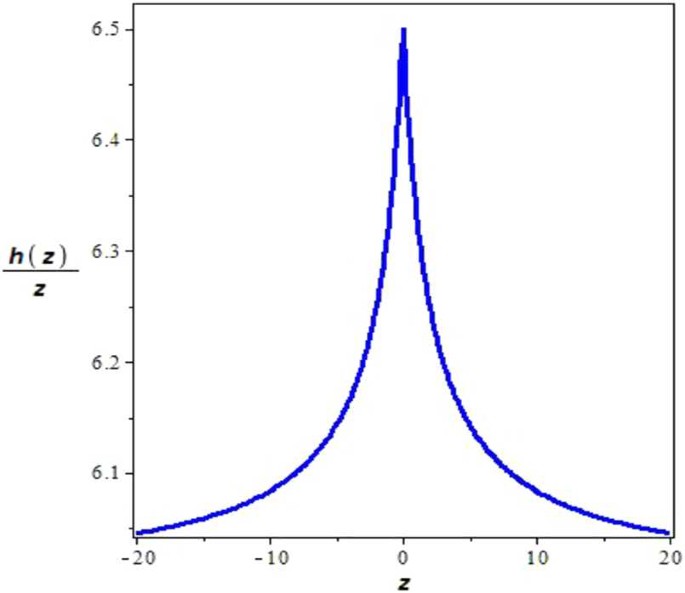
The function \(\frac {h(z)}{z}\) and its bounds for \(z\in [-20,20]\)
-
3.
The function
$$ \phi (y)=2y+\sin y, \quad \text{it tends to}\quad \frac{\phi (y)}{y}=2+ \frac{\sin y}{y}, \quad \text{for all } y\neq 0. $$Since \(-1\leq \frac{\sin y}{y}\leq 1\), then we get \(1\leq \frac{\phi (y)}{y}\leq 3\), and the derivative of the function \(\phi (y)\) with respect y becomes
$$ \bigl\vert \phi '(y) \bigr\vert = \vert 2+\cos y \vert \leq 3,\quad \text{for all } y\neq 0. $$Then we state that \(c=1\), \(c_{1}=3\), and \(M=3\). Path of the function \(\frac{\phi (y)}{y}\) is depicted in Fig. 2.
Figure 2 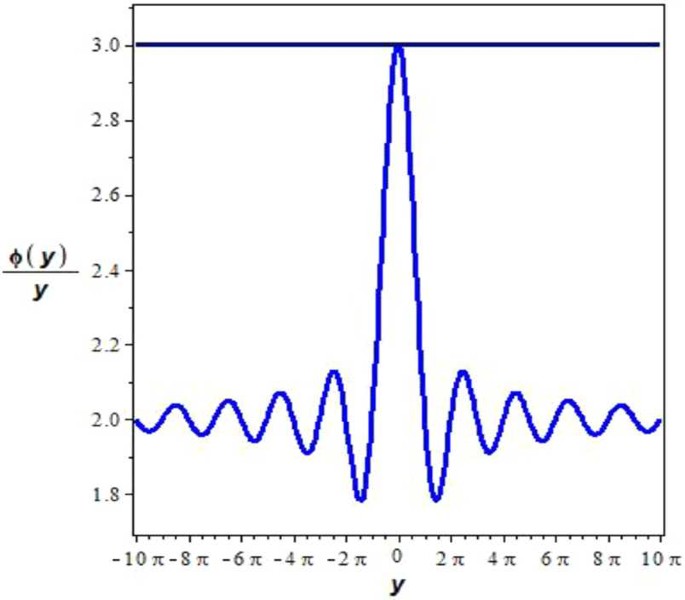
The function \(\frac {\phi (y)}{y}\) and its bounds for \(z\in [-10\pi ,10\pi ]\)
-
4.
The function
$$ f(x)=x+\frac{x}{1+x^{2}}, \quad \text{fulfills}\quad f(0)=0 \quad \text{and}\quad \frac{f(x)}{x}=1+\frac{1}{1+x^{2}}, \quad \text{for all } x\neq 0. $$As a result, \(1\leq \frac{f(x)}{x}\leq 2\), the derivative of the function f with respect to x is
$$ f'(x)=1+\frac{1-x^{2}}{(1+x^{2})^{2}}\leq 1+\frac{1}{1+x^{2}}\leq 2, \quad \text{and}\quad \bigl\vert f'(x) \bigr\vert \leq 2. $$It gives that \(\ell =1\), \(m=2\), and \(d=2\). Figure 3 shows the function \(\frac{f(x)}{x}\) and its bounds for \(x\in [-10,10]\).
Figure 3 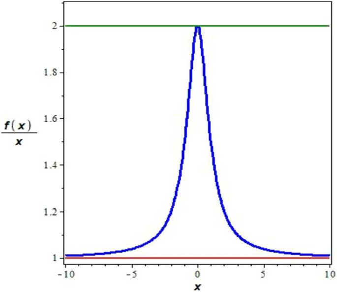
The function \(\frac {f(x)}{x}\) and its bounds for \(x\in [-10,10]\)
-
5.
Conditions \((iv)-\)(vi) of Theorem 2.1 have inequalities that are as follows:
$$\begin{aligned}& ab-c=11>0,\\& abc-c^{2}-a^{2}d=3\geq \delta . \end{aligned}$$Choose \(\delta =2.8\), then we can get the subsequent constants
$$\begin{aligned}& \delta _{0}=ab+bcd^{-1}=15>0,\\& 0.047\leq \varepsilon \leq \min \{24,1\}, \quad \text{it tends to}\quad 0.047 \leq \varepsilon \leq 1, \quad \text{here } \varepsilon =0.05 \text{ is chosen}. \end{aligned}$$Also,
$$ d_{1}=\varepsilon +\frac{1}{a}=0.55, \quad \text{and}\quad d_{2}= \varepsilon +\frac{d}{c}=2.05. $$Therefore, the condition \(2=a\ell >2(1+d_{1})\sigma ^{2}\cong 0.775\), is satisfied.
-
6.
The value of the constant r is such that
$$ r< 0.00497=\min \{0.038, 0.0395, 0.00497, 0.121\}. $$


As a result, all the elements above satisfy all of the requirements of Theorem 2.1.
Therefore, the zero solution of (3.1) is stochastically asymptotically stable.
4 Conclusions
This paper discusses a specific fourth-order nonlinear SDE with a constant delay. The paper obtains standard criteria for the stochastic asymptotic stability of the equation. The effectiveness of the functional used in the investigation greatly aids in proving the main result. The paper’s stochastic stability result enhances, incorporates, and supplements the existing stability results in the literature. Additionally, a relevant example is provided to verify the hypotheses.
Availability of data and materials
No data were generated or analyzed during the current study.
References
Ademola, A.T.: Periodicity, stability, and boundedness of solutions to certain fourth-order delay differential equations. Int. J. Nonlinear Sci. 28(1), 20–39 (2019)
Ademola, A.T.: Stability, boundedness and existence of unique periodic solutions to a class of fourth-order functional differential equation. Proyecciones 40(2), 251–283 (2021)
Ademola, T.A., Ogundiran, M.O.: On the existence and uniqueness of solutions of a generalized Lipschitz ordinary differential equations. Ife J. Sci. 9(2), 241–246 (2007)
Adesina, O.A., Ogundare, B.S.: Some new stability and boundedness results on a certain fourth-order nonlinear differential equation. Nonlinear Stud. 19(3), 359–369 (2012)
Balamuralitharan, S.: Periodic solutions of fourth-order delay differential equation. Bull. Iranian Math. Soc. 41(2), 307–314 (2015)
Burton, T.A.: Volterra Integral and Differential Equations. Academic Press, New York (1983)
Burton, T.A.: Stability and Periodic Solutions of Ordinary and Functional Differential Equations. Mathematics in Science and Engineering, vol. 178. Academic Press, Orlando (1985)
Cai, M., Meng, F.: Stability and boundedness of solutions for a certain fourth-order delay differential equation. Ann. of Appl. Math. 34(4), 345–357 (2018)
Driver, R.D.: Ordinary and Delay Differential Equations. Springer, New York (1976)
Fatmia, L., Remili, M., Rahmane, M.: On stability, boundedness and square integrability of solutions for fourth-order differential equations of neutral type with variable delay. Int. J. Nonlinear Anal. Appl. 14(1), 2169–2181 (2023). https://doi.org/10.22075/ijnaa.2022.27944.3764
Hale, J.K.: Theory of Functional Differential Equations. Springer, New York (1977)
Kang, H., Si, L.: Stability of solutions to certain fourth-order delay differential equations. Ann. Differ. Equ. 26, 407–413 (2010)
Korkmaz, E.: Stability and boundedness of solutions of nonlinear fourth-order differential equations with bounded delay. Sakarya Üniv. Fen Bilim. Enst. Derg. 21(6), 1317–1324 (2017)
Korkmaz, E.: Stability and square integrability of derivatives of solutions of nonlinear fourth-order differential equations with delay. J. Inequal. Appl. 2017, 134, 1–13 (2017)
Korkmaz, E., Tunç, C.: Boundedness and square integrability of solutions of nonlinear fourth-order differential equations with bounded delay. Electron. J. Differ. Equ. 2017, 47, 1–13 (2017)
Lakshmikantham, V., Wen, L., Zhang, B.: Theory of Differential Equations with Unbounded Delay. Springer, Berlin (1994)
Okoronkwo, E.O.: On stability and boundedness of solutions of a certain fourth-order delay differential equation. Int. J. Math. Math. Sci. 12(3), 589–602 (1989)
Rahmane, M., Oudjedi, L.D., Remili, M.: Stability, boundedness, and square integrability of solutions of neutral fourth-order differential equations. Armen. J. Math. 11(10), 1–17 (2019)
Rahmane, M., Remili, M.: On stability and boundedness of solutions of certain non autonomous fourth-order delay differential equations. Acta Univ. M. Belii Ser. Math. 23, 101–114 (2015)
Sadek, A.I.: On the stability of solutions of certain fourth-order delay differential equation. Appl. Math. Comput. 148, 587–597 (2004)
Sinha, A.S.C.: On stability of solutions of some third and fourth-order delay differential equations. Inf. Control 23, 165–172 (1973)
Tejumola, H.O., Tchegnani, B.: Stability, boundedness and existence of periodic solutions of some third-order and fourth-order nonlinear delay differential equations. J. Niger. Math. Soc. 19, 9–19 (2000)
Tunç, C.: On the uniform boundedness of solutions of some non-autonomous differential equations of the fourth-order. Appl. Math. Mech. 20, 622–628 (1999)
Tunç, C.: On stability of solutions of certain fourth-order delay differential equations. Appl. Math. Mech. 27, 1141–1148 (2006)
Tunç, C.: A boundedness criterion for fourth-order nonlinear ordinary differential equations with delay. Int. J. Nonlinear Sci. 6, 195–201 (2008)
Yoshizawa, T.: Stability Theory by Liapunov’s Second Method. The Mathematical Society of Japan (1966)
Yoshizawa, T.: Stability Theory and Existence of Periodic Solutions and Almost Periodic Solutions. Springer, New York (1975)
Funding
Open access funding provided by The Science, Technology & Innovation Funding Authority (STDF) in cooperation with The Egyptian Knowledge Bank (EKB).
Author information
Authors and Affiliations
Contributions
All authors contributed equally and significantly in writing this article.
Corresponding author
Ethics declarations
Competing interests
The authors declare no competing interests.
Additional information
Publisher’s Note
Springer Nature remains neutral with regard to jurisdictional claims in published maps and institutional affiliations.
Rights and permissions
Open Access This article is licensed under a Creative Commons Attribution 4.0 International License, which permits use, sharing, adaptation, distribution and reproduction in any medium or format, as long as you give appropriate credit to the original author(s) and the source, provide a link to the Creative Commons licence, and indicate if changes were made. The images or other third party material in this article are included in the article’s Creative Commons licence, unless indicated otherwise in a credit line to the material. If material is not included in the article’s Creative Commons licence and your intended use is not permitted by statutory regulation or exceeds the permitted use, you will need to obtain permission directly from the copyright holder. To view a copy of this licence, visit http://creativecommons.org/licenses/by/4.0/.
About this article

Cite this article
Mahmoud, A.M., Adewumi, A.O. & Ademola, A.T. Stochastic stability of solutions for a fourth-order stochastic differential equation with constant delay. J Inequal Appl 2023, 148 (2023). https://doi.org/10.1186/s13660-023-03061-6
Received:
Accepted:
Published:
DOI: https://doi.org/10.1186/s13660-023-03061-6