
Abstract
Baryon and lepton numbers being accidental global symmetries of the Standard Model (SM), it is natural to promote them to local symmetries. However, to preserve anomaly-freedom, only combinations of B–L are viable. In this spirit, we investigate possible dark matter realizations in the context of the \(U(1)_\mathrm{B{-}L}\) model: (i) Dirac fermion with unbroken B–L; (ii) Dirac fermion with broken B–L; (iii) scalar dark matter; (iv) two-component dark matter. We compute the relic abundance, direct and indirect detection observables and confront them with recent results from Planck, LUX-2016, and Fermi-LAT and prospects from XENON1T. In addition to the well-known LEP bound \(M_{Z^{\prime }}/g_\mathrm{BL} \gtrsim 7\) TeV, we include often ignored LHC bounds using 13 TeV dilepton (dimuon + dielectron) data at next-to-leading order plus next-to-leading logarithmic accuracy. We show that, for gauge couplings smaller than 0.4, the LHC gives rise to the strongest collider limit. In particular, we find \(M_{Z^{\prime }}/g_\mathrm{BL} > 8.7\) TeV for \(g_\mathrm{BL}=0.3\). We conclude that the NLO+NLL corrections improve the dilepton bounds on the \(Z^{\prime }\) mass and that both dark matter candidates are only viable in the \(Z^{\prime }\) resonance region, with the parameter space for scalar dark matter being fully probed by XENON1T. Lastly, we show that one can successfully have a minimal two-component dark matter model.
1 Introduction
The availability of data from collider, direct and indirect searches for dark matter has raised the importance of dark matter complementarity across these search strategies. In this context, effective field theories and simplified models have become popular tools, as they can capture most of the dark matter phenomenology. Planck measurements of the power spectrum of the cosmic microwave background radiation infer that the cold dark matter abundance should be around 27% (\(\Omega _\mathrm{DM} h^2=0.12\)), where h is a parameter that accounts for uncertainties in the Hubble rate [1]. This alone strongly constrains the viable parameter space of dark matter models. The observation of cosmic rays and gamma rays also offers a compelling probe for dark matter [2,3,4,5,6,7,8,9,10,11,12,13,14]. In particular, the Fermi-LAT sensitivity to continuous gamma-ray emission from dark matter annihilations taking place in dwarf galaxies resulted in restrictive bounds in the annihilation cross section today, namely \(\sigma v < 3 \times 10^{-26}\,\, \mathrm{cm^3/s}\) for masses of 80 GeV and annihilation into \(b\bar{b}\) quark pairs [15]. This rules out a multitude of light weakly interacting massive particle (WIMP) models in which velocity-independent interactions occur.
Moreover, underground detectors using liquid xenon, such as XENON [16] and LUX [17] that use scintillation and ionization measurements to discriminate signal from background events, observed no excess, leading to the exclusion of spin-independent WIMP–nucleon scattering cross sections larger than \(10^{-45}\,\, \mathrm{cm^2}\) for WIMP masses of 50 GeV. Other experiments have placed complementary limits in particular at lower masses such as SUPERCDMS, which uses Ge targets [18]. The ongoing XENON1T [19] and LZ [20] experiments are expected to bring down the limits by roughly two orders of magnitude in the absence of signal and zero background events.
Besides the indirect and direct detection probes, the Tevatron [21] and the LHC [22, 23] have proven to be great laboratories to test dark matter models. In the case where the dark and visible sectors are connected by vector mediators, dijet [24,25,26,27] and dilepton [28,29,30,31,32] bounds are by far the most stringent constraints. Dark matter phenomenology is then dictated by gauge interactions which are determined, once the gauge group behind the origin of the vector mediator is known. The common approach is to consider simplified Lagrangians that encompass both Dirac and Majorana dark matter fermions and then to compute dark matter observables; namely, relic density, annihilation and scattering cross sections, the latter being spin-independent and spin-dependent for Dirac and Majorana fermions, respectively.Footnote 1 The simplified dark matter model approach is interesting, intuitive and serves as a guide for future work. However, the Lagrangians involved might lead to different results once embedded in a complete theory.
In the context of the B–L model, dark matter scenarios have been previously investigated. In [33] the authors discussed a limited region of the parameter space of scalar dark matter only. In [34], the authors discussed the radiative see-saw mechanism to account for neutrino masses and focused exclusively on dark matter abundance. Supersymmetric B–L extensions [35,36,37] and a conformal approach [38] have also been investigated. Even though later disfavored in [39], a global B–L symmetry has been proposed [40]. In [41] a warm dark matter scenario was investigated. The possibility of having one of the right-handed neutrinos to be the dark matter candidate was entertained in [42,43,44], whereas in [45] an additional scalar played this role. This extra scalar dark matter was also investigated in [46], but in the context of classical scale invariance. The authors of [47, 48] considered an exotic B–L model and advocated the presence of many scalar fields. Finally, the authors of [49] studied Dirac fermion dark matter in the context of a \(U(1)_\mathrm{B{-}L}\) symmetry, but with the inclusion of LEP bounds only they discussed gamma-ray lines emissions, which turned out to be irrelevant unless one lives very close to the resonance with a dark matter quantum number under B–L larger than 3.
Thus, our work supplements previous studies for the following reasons:
-
(i)
Both fermionic and scalar dark matter realizations are discussed as well as several quantum numbers and gauge couplings options.
-
(ii)
We investigate two-component dark matter scenarios.
-
(iii)
We perform a detailed collider study at next-to-leading order (NLO) plus next-to-leading logarithmic (NLL) accuracy using recent dilepton data from the LHC at 13 TeV, which are often ignored due to the handy LEP limits.
-
(iv)
Finally, the region of parameter space allowed/excluded by limits from the LHC, LEP and indirect detection experiments in dependence of the mass of the mediator, gauge couplings and dark matter mass is presented.
2 Model
In the Standard Model, both baryon and lepton numbers are accidental global symmetries. Thus, a natural extension of the SM consists of gauging both quantum numbers. However, only combinations of B–L are free of triangle anomalies. Interestingly, the gauge anomalies \(\mathrm{Tr}(U(1)_\mathrm{B{-}L} SU(2)_L^2), \mathrm{Tr}(U(1)_\mathrm{B{-}L} U(1)_Y^2)\) and \(\mathrm{Tr}(U(1)_\mathrm{B{-}L}^3)\) vanish with the introduction of three right-handed neutrinos having charge \((-1)\) under B–L. In addition, this also leads to vanishing gravitational anomalies. Therefore, the gauged B–L symmetry naturally addresses neutrino masses through see-saw mechanisms [50,51,52,53,54,55]. There are several ways to accommodate dark matter without spoiling the anomaly cancelation, namely:
-
(i)
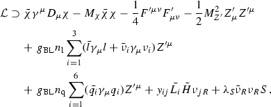
Dirac fermion dark matter—\(Z^{\prime }\) portal with unbroken B–L This model introduces a vector-like Dirac fermion charged under \(U(1)_\mathrm{B{-}L}\) leaving the B–L symmetry unbroken. Dark matter phenomenology is then governed by the \(Z^{\prime }\) portal. The new gauge boson mass is generated through the Stueckelberg mechanism, which leads to the following Lagrangian [56,57,58]:
 (2.1)
(2.1)where \(n_\mathrm{q}=1/3\), \(n_\mathrm{l}=-1\), \(D_{\mu }\chi =(\partial _{\mu } +i g_\mathrm{BL} n_{\chi }Z_{\mu }^{\prime })\chi \). We denote by \(\tilde{H}\) the isospin transformation of the Higgs doublet, \(H=(\phi ^+, \phi ^0)^T\), defined as \(\tilde{H}= i\sigma _2 H\). The dark matter charge, \(n_{\chi }\), should be different from \(\pm 1\) to prohibit an additional Yukawa term involving \(\chi _R\), which would lead to dark matter decay. Note that \(M_{Z^{\prime }}\) is not determined by the B–L symmetry and that the right-handed neutrinos acquire mass through the usual Yukawa term. Consequently, the neutrinos are Dirac fermions with their small masses being obtained via suppressed Yukawa couplings. We emphasize that the dark matter stability is guaranteed by B–L symmetry.
-
(ii)
Dirac fermion dark matter—\(Z^{\prime }\) portal with broken B–L In this scenario one adds an SM singlet scalar, S, carrying charge 2 under the B–L symmetry. Dark matter is realized via a vector-like Dirac fermion \(\chi \) as follows:
 (2.2)
(2.2)where \(v_\mathrm{BL}\) is the vev of the singlet scalar S and \(M_{Z^{\prime }} = 2 g_\mathrm{BL} v_\mathrm{BL}\). This mass term arises after spontaneous symmetry breaking of the B–L symmetry through the scalar S. The mass of the new gauge boson is generated through the kinetic term of the scalar. Interestingly, in this procedure the neutrinos are Majorana particles. The right-handed neutrinos have masses determined by the last term in Eq. (2.2), whereas the active neutrinos have their masses generated through the usual see-saw type I mechanism. The dark matter stability in this case is ensured by a \(Z_2\) symmetry remnant from the B–L spontaneous symmetry breaking. Another possibility would be to give different charges to the three right-handed neutrinos such as \((5,-4,-4)\), which is still anomaly-free. However, several extra fields are then needed to successfully generate neutrino masses [59]. For other different studies based on the B–L gauge symmetry, see [34, 60,61,62,63,64,65,66,67,68].
-
(iii)
Scalar dark matter—\(Z^{\prime }\) portal Scalar dark matter in the context of B–L symmetry is also a plausible alternative to accommodate dark matter, since it requires only two new fields: a singlet scalar S, with charge \(+2\) under B–L, and a scalar \(\phi \), as dark matter which should be charged under B–L with a quantum number, \(n_{\phi }\), different from multiples of \(\pm 2\) for stability purposes [45]. Taking this into account, the Lagrangian of this model reads
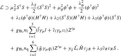 (2.3)
(2.3)The dark matter phenomenology [45] is determined by both gauge interactions, \(\phi ^{\dagger }\phi \rightarrow Z^{\prime } \rightarrow \bar{f}f\), and scalar interactions, \(\phi ^{\dagger }\phi \rightarrow h \rightarrow \bar{f}f, SS\). In the first case the dark matter phenomenology is strongly related to the gauge coupling and the \(Z^{\prime }\) mass. It is very predictive and connected to collider physics. In the second, the scalar potential couplings control dark matter observables and the strong connection to collider physics is lost, therefore, we will not discuss it further. For a detailed study see e.g. [45].


Dark matter annihilation and dark matter–nucleon scattering processes in the fermion dark matter model, where f stands for all SM fermions and q represents the quarks. The t-channel annihilation process is only relevant for \(M_{\chi } > M_{Z^{\prime }}\)
3 Dark matter abundance
The relic abundance of dark matter is determined by solving the Boltzmann equation. The dark matter particle pair annihilates and is pair-produced in equal rate in the early Universe, but as the Universe cools down and expands, eventually the expansion rate approaches the interaction rate, and from then on the dark matter particles are only able to self-annihilate into lighter particles. Eventually, then the expansion rate prevents the dark matter particles from self-annihilating. This episode is referred to as freeze-out. In order words, the abundance of left-over dark matter particles is linked to the annihilation cross section at the freeze-out, which can be very different from the annihilation cross section today [69]. Thus, the stronger the annihilation cross section is, the fewer remnant dark matter particles subsist today. In what follows, we discuss the abundance of the fermion and scalar dark matter in quantitative terms.
Let n be to number density and s the entropy of the Universe, in general terms, the relic density calculation entails solving the Boltzmann equation that computes the dark matter abundance at a given temperature, \(Y(T)=n/s\), found to be [70, 71],
where \(g_{*}(T)\) is the temperature dependent number of degrees of freedom, \(M_p\) is the Planck mass, \(Y_\mathrm {eq}(T)\) the dark matter abundance in thermal equilibrium, \(\langle \sigma v\rangle \) the thermally averaged dark matter annihilation cross section. In general terms the annihilation reads [71]
where \(g_i\) is the number of degrees of freedom of the dark matter particle, \(\sigma _{ij;kl}\) the total cross section for annihilation of a pair of particles with masses \(m_i\), \(m_j\) into the final states (k, l), and \(p_{ij}(\sqrt{s})\) is the momentum of the incoming dark matter particles in their center-of-mass frame. For instance, today the dark matter particles are non-relativistic and thus \(\sqrt{s}\) is simply twice the dark matter mass. \(K_1 (K_2)\) are the modified Bessel functions of order one and two, respectively. In order to obtain the dark matter abundance today, \(Y(T_0)\), we integrate Eq. (3.1) from \(T=\infty \) to \(T=T_0\), leading to

Dirac fermion. Abundance as a function of mass for various gauge couplings and \(Z'\) boson masses. Because the model must satisfy the relic density, it features a strong dependence in the resonance region

Dark matter annihilation and dark matter–nucleon scattering processes in the scalar dark matter model
In what follows we have numerically computed the dark matter abundance within micrOMEGAS [72, 73]; however, we do present analytic expressions for the annihilation cross section since they help us understand the relevant processes and our numerical results.
3.1 Dirac fermion
In Fig. 1a, b, we show the processes that set the dark matter abundance for the fermion. When \(M_{\chi } < M_{Z^{\prime }}\), only the first diagram is relevant. f stands for all SM fermions, including the right-handed neutrinos, whose masses are in the eV range in the case where the B–L symmetry in unbroken, whereas in the broken B–L scenario their masses are kept at 100 GeV. The precise value for their masses is not relevant, and both cases lead to very similar dark matter phenomenology. For this reason, dark matter observables will be derived without explicitly specifying whether or not the B–L symmetry is broken.
That said, the annihilation cross section into a pair of SM fermions through (assuming that \(m_\chi > m_\mathrm{f}\)) is found to be
while the annihilation into \(Z^{\prime }\) gauge bosons for \(m_\chi > m_{Z^{\prime }}\) is
where \(n_\mathrm{f}\) is the SM fermion charged under B–L, v is the relative velocity of the annihilating dark matter pair and \(n_c\) is the number of colors of the final state SM fermion. The \(Z^{\prime }\) width reads
where \(\theta \) is the unit step function.
In Fig. 2 we display, for \(n_{\chi }=1/3\), the abundance of the fermion as a function of its mass. In the left panel, Fig. 2a, the \(Z^{\prime }\) mass has been fixed to 4 TeV and the gauge coupling varied in \(g_\mathrm{BL}\in [0.1,0.8]\), while in the right panel, Fig. 2b, we keep \(g_\mathrm{BL}=0.1\) and vary \(M_{Z^{\prime }}=2,4,6\) TeV.
From Fig. 2a, it is clear that the increase in the coupling widens the resonance and therefore leads to viable dark matter masses away from \(M_{Z^{\prime }}/2\), lower or higher. In addition, the larger the coupling, the larger the annihilation rate, leading to smaller abundance. Thus, one needs sufficiently large gauge couplings to enhance the annihilation rate and reach \(\Omega h^2 \sim 0.1\). Notice that the resonance condition is not needed, if couplings close to unity are used. Such large couplings arise naturally in 3-3-1 models [28, 74,75,76,77,78,79,80,81] and left–right models [50, 53, 82,83,84,85,86,87,88,89]. Other fermion dark matter models feature similar trends [90,91,92,93,94].
The impact of the \(Z^{\prime }\) mass is shown in Fig. 2b, which exhibits a series of peaks at different dark matter masses. The larger \(M_{Z^{\prime }}\) gets, the heavier the dark matter mass has to be in order to achieve the right abundance. We point out that both results for fermion dark matter are presented for \(n_\chi =1/3\), but they can easily be rescaled, since the abundance scales as \(n_\chi ^2 g_\mathrm{BL}^4\). Hence, for constant relic density, a change in \(n_\chi \) straightforwardly induces a quadratically inverse change in \(g_\mathrm{BL}\).
By looking at Eqs. (3.4)–(3.5) we notice that in the limit in which \(M_{\chi } > M_{Z^{\prime }}\) we can see that the annihilation into \(Z^{\prime }\) gauge bosons is comparable with the annihilation into fermion pairs, but the scaling with the gauge coupling, \(g_\mathrm{BL}\), and the dark matter mass continue to be the same. For this reason we do not see a change in shape in Fig. 2a, b when \(M_{\chi } \sim M_{Z^{\prime }}\).
3.2 Scalar field
In Fig. 3a–c we show the Feynman diagrams relevant for determining the scalar dark matter abundance. In Fig. 4 the abundance for two different charges under B–L, \(n_\phi =1/3\) and \(n_\phi =1\), is shown. The results can be understood knowing the analytic expressions for the annihilation cross sections. The annihilation cross section into fermions reads
where \(n_c^f\) is number of colors of the final state particle, \(n_\mathrm{f}\) is the SM fermion charged under B–L, whereas the annihilation into \(Z^{\prime }Z^{\prime }\) is found to be
which in the limit \(M_{\phi } \gg M_{Z^{\prime }}\) leads to

Scalar field. Abundance as a function of mass. The kinks in the plots are the result of the \(Z^{\prime }\) threshold, i.e. when the scalar can pair annihilate to produce \(Z^{\prime }\) bosons
As expected the annihilation cross sections are proportional to \(g_\mathrm{BL}^4\). The annihilation into fermions gets an \(n_{\phi }\) factor in one side of the vertices and \(n_{f}\) in the other, rendering the annihilation cross section to scale as \(g_\mathrm{BL}^4 n_{\phi }^2 n_\mathrm{f}^2\). The annihilation into \(Z^{\prime } Z^{\prime }\) has two contributions, however. The t-channel and four-point interactions are all derived from the covariant derivative and scale as \(g_\mathrm{BL}^4 n_{\phi }^4\). Having these expressions at hand a few remarks are in order.
-
(i)
The annihilation into fermions is velocity suppressed. Its contribution for the relic density might be relevant, but today \(v \sim 10^{-3}\), rending its contribution to be rather small.
-
(ii)
The values adopted for the B–L charged \(n_\phi \) and \(n_\mathrm{f}\) dictate which channel is the most relevant for the relic density;
-
(iii)
The values we used for \(n_\phi \) and \(n_\mathrm{f}\), lead to a sizable annihilation into \(Z^{\prime }Z^{\prime }\), and for this reason we observe kinks in Fig. 4 whenever \(M_{\phi } \sim M_{Z^{\prime }}\). This effect is also present, but much less pronounced in the fermion case previously discussed.
-
(iv)
Due to the velocity suppression in Eq. (3.7), one can check that the annihilation into \(Z^{\prime }Z^{\prime }\) is dominant today.

Dirac fermion. Spin-independent dark matter–nucleon scattering cross section as a function of the dark matter mass with \(n=1/3\) and \(M_{Z^{\prime }}=4,6\) TeV for different gauge couplings, \(g_\mathrm{BL}=0.1,0.4,0.8\). The current limit from LUX-2015 (solid line) [100], preliminary limit from LUX-2016 (dotted-dashed) [101] and the one projected from XENON1T (dashed line) for 2 years of data taking [19] are also shown
Looking at Fig. 4, we conclude that the s-channel resonance regime \(M_{\phi } \sim M_{Z^{\prime }}/2\) is responsible for increasing the annihilation cross section and consequently reducing the abundance to values close to the one inferred by Planck. Figure 4c shows the abundance with \(n=1\) and \(g_\mathrm{BL}=0.8\) and for various masses of the new gauge boson, \(M_{Z^{\prime }}=2,4,6\) TeV. Again, the effect of increasing \(M_{Z'}\) is to simply move the resonance region to higher dark matter masses. It is noticeable that for \( g_\mathrm{BL}=0.8\) the resonance region is wide enough to accommodate two different dark matter masses yielding the right abundance.
As already mentioned, the annihilation cross section grows as \(n_\phi ^2 g_\mathrm{BL}^4\). For \(n_\phi \ll 1\), one therefore needs gauge couplings larger than 1 in order to satisfy the relic density constraint. On the other hand, values of \(n_\phi \) closer to 1 enhance the dark matter–nucleon scattering rate, thus severely restricting the model, as we shall see below.
In principle one could also probe this model with cosmic-ray and gamma-ray data [2, 4,5,6,7,8,9,10,11,12,13, 95,96,97,98,99]. In particular, one could use gamma-ray observations of dwarf galaxies from the Fermi-LAT satellite to constrain the annihilation cross section into SM fermions, which after hadronization processes produce gamma rays [15]. Although, as we shall see further, only heavy dark matter particles are viable, much heavier than 100 GeV, the indirect detection limits are rather subdominant to collider and direct detection ones and for this reason we have not shown them.
As a summary, we have seen in this part that both Dirac fermions and scalars can be viable dark matter candidates of the Universe as long as the annihilation rate occurs not very far from the resonance. It is time to derive the direct detection limits.

Scalar field. Scattering cross section as a function of the dark matter mass for \(n=1\) and various values of \(M_{Z'}\) and coupling \(g_\mathrm{BL}\). Predictions are compared to current and projected bounds from LUX-2015 (solid), LUX-2016 (dotted-dashed) and XENON1T (dashed)
4 Direct dark matter detection
Direct dark matter detection relies on the measurement of nuclear recoil energies down to energies below 10 keV. The method is based on the use of discriminating variables such as ionization, heat, and scintillation efficiencies to disentangle possible dark matter events from nuclear background rates and mis-identified electron recoils; see [102,103,104,105,106,107] for recent reviews. The measurement of the recoil energy is translated into the plane dark matter–nucleon scattering cross section vs. mass, once the dark matter velocity distribution and the local density is set. Since no excess of events has been observed, only limits in this same plane have been derived. The LUX experiment provides the world-leading limits on both the spin-independent and the spin-dependent scattering cross sections, with the former being more stringent, which we refer to as LUX2015 in the figures. However, LUX recently presented their new limit with 332 live days, which improves by a factor of 4 the latest one [108]. It is the latter bound that one finds incorporated in the figures with a dotted-dashed line, labeled LUX2016.
Since, in our setup, both Dirac fermion and scalar dark matter models exhibit larger spin-independent rates, we will use the spin-independent bounds. Moreover, we present the projected bounds from the ongoing XENON1T experiment, which is expected to surpass the LUX2015 sensitivity by two orders of magnitude with two years of data taking [19].
The analytic expressions for the spin-independent WIMP–nucleon scattering cross section for both scalar and Dirac fermion are identical in the B–L models under study and they read
where \(DM=\chi ,\phi \), and \(m_\mathrm{n}\) is the nucleon mass.
Having in mind this expression we discuss the results for dark matter–nucleon scattering cross sections for both candidates.
4.1 Dirac fermion
In Fig. 1c we show the Feynman diagram responsible for dark matter–nucleon scattering. Figure 5 shows the spin-independent dark matter–nucleon scattering cross section as a function of the dark matter mass with \(n_\chi =1/3\) and \(M_{Z^{\prime }}=4\) TeV (Fig. 5a) and \(M_{Z'}=6~\)TeV (Fig. 5b) for different gauge couplings \(g_\mathrm{BL}\in \{0.1,0.4,0.8\}\). In both figures, current limits from LUX2015 (solid line) [100], LUX2016 [108], and projected limits from XENON1T (dashed line) are superimposed. The curves read from top to bottom: blue is for \(g_\mathrm{BL}=0.8\), red for \(g_\mathrm{BL}=0.4\), and pink for \(g_\mathrm{BL}=0.1\). The dark blobs in the figure reproduce the right relic abundance.
From Fig. 5a, it is clear that one needs to use gauge couplings smaller than 0.8 in order to have a viable dark matter candidate with masses below 2 TeV. If no dark matter signal is seen, the XENON1T experiment is expected to exclude gauge coupling values larger than 0.4, if the dark matter mass is demanded to be below 8 TeV. Ramping up the \(Z^{\prime }\) mass to 6 TeV ameliorates the situation, and couplings as low as 0.8 can be allowed in the entire mass range. This range will, however, be entirely probed by XENON1T, whereas this experiment will only probe dark matter masses below 1.5 TeV for a coupling of 0.4.

Inclusive total cross section for \(pp\rightarrow Z'\rightarrow \ell \bar{\ell }\) at NLO+NLL in the \(\mathrm {U(1)}_\mathrm{B{-}L}\) models for various values of \(g_\mathrm{B{-}L}\) as a function of the mass of the heavy resonance \(M_{Z'}\)
4.2 Scalar field
In Fig. 6 we display the scattering cross section as a function of the dark matter mass with \(n_\phi =1\) and various values of the new gauge boson mass, \(M_{Z^{\prime }}\in \{2,4\}\) TeV, and gauge couplings, \(g_\mathrm{BL}\in \{0.1,0.4,0.8\}\). In both plots, Fig. 6a, b, the predictions are compared with current bound from LUX2015 (solid), from LUX2016 (dotted-dashed), and projected from XENON1T (dashed). The blobs represent points with the right relic density. The value of \(n_\phi =1\) has been selected in order to simplify the identification of points satisfying the correct dark matter abundance. As before, results can be rescaled taking into account the scaling of the scattering cross section, \(n^2_\phi g_\mathrm{BL}^4/M_{Z^{\prime }}^4\). That is, the result, for \(n_\phi =1,\ g_\mathrm{BL}=0.4\), is equivalent to the one with \(n_\phi =1/3\) and \(g_\mathrm{BL}=0.7\).
From Fig. 6a, one sees that LUX2015 already ruled out a large region of the model parameter space, forcing the use of suppressed gauge couplings, e.g. \(g_\mathrm{BL} \sim 0.1\), for \(M_{Z^{\prime }}=2\) TeV. Note also that the projected limits from XENON1T might fiercely exclude couplings larger than 0.1.
Similarly, Fig. 6b shows the spin-independent cross section as a function of the dark matter mass for various values of \(M_{Z'}\) and fixed \(g_\mathrm{BL}=0.4\) and \(n_\phi =1\). The LUX experiment excludes \(Z^{\prime }\) masses above 4 TeV, whereas XENON1T has the potential to rule out masses larger than 6 TeV, which is in the ballpark of the LHC-14 TeV sensitivity to gauge bosons with an integrated luminosity of 300 fb\(^{-1}\) [109, 110]. Analogous conclusions would be drawn for \(n_\phi =1/3\) by simply shifting the gauge coupling as mentioned before.
It is important to keep in mind that collider bounds on the model have been ignored up to now. Including them would lead to the exclusion of some of the points considered above. These limits will be included later on, when we present our results in a more informative plane, that is, \(M_{Z^{\prime }}\) vs. \(g_\mathrm{BL}\). In what follows, we derive updated limits on the mass of a new neutral gauge boson using 13 TeV dilepton data from the LHC and compare with the well-known LEP bounds.
5 Collider limits
Since our models feature sizable couplings to charged leptons and observables dictated by the \(Z^{\prime }\) gauge boson, searches for dark matter at the LHC, also known as mono-X searches, are subdominant compared to the resonance searches in the channels with two jets and two charged leptons [26, 111, 112]. The ATLAS and CMS collaborations have performed extensive analyses to search for new heavy resonances in both dilepton and dijet signals. In the absence of any excess event over the Standard Model background, the two experiments derived lower bounds on the mass of the \(Z'\)-boson, with dileptons offering stronger limits than dijets due to relatively fewer background events. These bounds are limited to a given model, and typically the experiments express their results assuming simplified models such as the Sequential SM (SSM) or the GUT-inspired \(\mathrm {E}_6\) models.
In this work, however, we re-interpreted their results in terms of the B–L model in question.Footnote 2 In particular, the ATLAS collaboration [114] analyzed 3.2 fb\(^{-1}\) of pp collisions at \(\sqrt{s}=13\) TeV searching for new phenomena in the dilepton final state and extracted the limit \(M^\mathrm{SSM}_{Z'}\ge 3.4\) TeV.Footnote 3 To calculate the total production cross section of a heavy neutral resonance \(Z'\) and its subsequent decay into leptons, we use the public code RESUMMINO [115], in which we implemented the appropriate couplings. RESUMMINO implements threshold resummation for total cross sections, \(p_T\)-resummation for the \(p_T\) distribution of heavy gauge bosons, as well as a joint resummation matched to the fixed-order NLO calculation.
When it comes down to interpreting dilepton resonance searches from ATLAS to a model different from the ones aforementioned, one needs to carefully compute the propagator width. In the B–L model, the width, \(\Gamma _{Z^{\prime }}\) is proportional to \(g_\mathrm{BL}^{2} M_{Z'}\) and was estimated using PYTHIA 8.215 [116, 117]. The following relation was found:
to a very good precision. Therefore, it is clear that, for any perturbative values of \(g_\mathrm{BL}\), the \(Z'\)-boson can be considered as a narrow resonance. For our numerical study we use the CT14 [118] NLO PDF set with \(\alpha _{S}(M_Z)=0.118\). Following [114], we cut on the invariant mass of the lepton pair, \(q_{\ell \ell }^2 \ge 500\) GeV. For each value of mass, \(M_{Z'}\), the electroweak coupling constant \(\alpha _{EW}\) is evolved to \(\alpha _{EW}(M_{Z'}^2)\). Finally, we set the factorization and renormalization scales such that \(\mu _F=\mu _R=M_{Z'}\). With these settings, we were able to reproduce to a good level (\(\sim \)2–3%) the ATLAS predictions for the SSM.

LHC exclusion limits for the \(\mathrm {U(1)}_\mathrm{B{-}L}\) model
In Fig. 7, we show the inclusive total cross section for the process, \(pp\rightarrow Z'\rightarrow \ell \bar{\ell }\) calculated at NLO+NLL for the B–L model for various values of the gauge coupling \(g_\mathrm{B{-}L}\) and as a function of the mass of the heavy resonance. From this, it is straightforward to estimate the lower bound on the mass of the resonance. In Fig. 8a, we exhibit this limit in the plane \(M_{Z'}\) vs. \(g_\mathrm{BL}\), while Fig. 8b shows the same limit in the plane \(M_{Z'}/g_\mathrm{BL}\) vs. \(g_\mathrm{BL}\).
Comparing with the SSM result obtained by ATLAS, we see that the exclusion bound for the B–L model is weaker. Note that in a recent analysis [46] the LHC bounds for \(\sim 5\) fb\(^{-1}\) of data and 8 TeV center-of-mass energy were computed. The conclusion was that for \(M_{Z^{\prime }} < 3\) TeV the LHC bounds are stronger than those from LEP, which is in very good agreement with our results obtained at 13 TeV with \(3.2\, \mathrm{fb^{-1}}\) of data. For the SSM, ATLAS results for 13 TeV with 3.2 fb\(^{-1}\) are a bit stronger than those at 8 TeV and \(20\, \mathrm{fb^{-1}}\), which uses much more data than the analysis in [46]. In addition, our results rely on the inclusion of NLO+NLL order effects, which improves our limits. Thus, the collider limits in [46] seem to be overoptimistic. Moreover, an assessment of the LHC sensitivity to the B–L model at 13 TeV, was recently performed in [119] without inclusion of detector effects and NLO corrections, and did not perform a detailed dark matter phenomenology. There, the authors have found a limit much stronger than ours, namely \(M_{Z^{\prime }} > 3\) TeV for \(g_\mathrm{BL}=0.01\).
We point that in the regime which \(M_{Z^{\prime }} > 2 m_{\chi }\), the invisible decay is open, but we checked this does not induce meaningful changes to our bounds in agreement with [30] and this fact can be easily understood. First note that, if one breaks down the total \(Z^{\prime }\) decay width into several terms, one finds
with \(\Gamma _\mathrm{l},\Gamma _\nu , \Gamma _\mathrm{q}\) and \(\Gamma _{\chi }\) being the individual decay widths of a charged lepton, neutrino flavor, quark, and dark matter, respectively, where we have factorized the dependence on the quantum number. In the limit \(M_{Z^{\prime }} > 2 m_{\chi }\), the individual decay widths are all similar, and thus the total decay width does not change much with the opening of the dark matter channel as well as the branching ratio into charged leptons, which is relevant for our bounds. Consequently the dilepton limit on the \(Z^{\prime }\) mass is mildly dependent on the dark matter mass. If the coupling strength of dark matter particle with the \(Z^{\prime }\) could be arbitrarily large and independent of the couplings to SM fermions, then the total width of the \(Z^{\prime }\) boson could be altered. See [120,121,122,123,124] for discussions on the topic.
We are now ready to combine the relic density, direct detection and collider constraints in the model. To do so, perhaps it is more informative to gather the results in the plane \(M_{Z^{\prime }}\) vs. \(g_\mathrm{BL}\), since these two parameters basically define the B–L symmetry.

Allowed region of parameters for a 1 TeV Dirac fermion as dark matter. The green curve delimits the region of parameter space with the right abundance (\(\Omega h^2=0.11{-}0.12\)), the pink (gray) shaded region is ruled out by LUX2016 (XENON1T), the blue region is excluded by dilepton data from the LHC, and the solid red (dashed) lines represent the current (old) LEP-II bounds, namely \(M_{Z^{\prime }}/g_\mathrm{BL}> 7\) TeV (\(M_{Z^{\prime }}/g_\mathrm{BL}> 6\) TeV)
6 Combined results
6.1 Dirac fermion
In this section we outline the viable parameter space in an arguably more informative plane, i.e. \(M_{Z^{\prime }}\) vs. \(g_\mathrm{BL}\) with charge \(n_\chi =1/3\) under B–L throughout. We combine our findings from relic density, direct detection and collider searches for both the Dirac fermion and the scalar dark matter models.
In all figures, the green curve delimits the region of parameter space yielding the right abundance (\(\Omega h^2=0.11-0.12\)), the pink (gray) shaded region is excluded by LUX2016 (XENON1T), the blue region is ruled out by dilepton data from the LHC, and the solid red (dashed) lines represent the current (old) LEP-II bounds, namely \(M_{Z^{\prime }}/g_\mathrm{BL}> 7\) TeV (\(M_{Z^{\prime }}/g_\mathrm{BL}> 6\) TeV).
In Fig. 9 we collect these results for a 1 TeV Dirac fermion, which features a \(Z^{\prime }\) resonance of 2 TeV. Since the annihilation cross section grows with \(n_{\chi }^2 g_\mathrm{BL}^4/(4m_{\chi }^2-M_{Z^{\prime }}^2)^2\), we can see that for small gauge couplings one needs to live very close to the resonance to obtain the right relic density, but as we increase the coupling, the regions relatively far from the resonance become viable. The annihilation cross section is typically small, leading to overabundant dark matter. Therefore one needs to either use large gauge couplings or be near the resonance region to increase the annihilation cross section and bring down the relic abundance to the correct value. Interestingly, LUX2016 limits on the spin-independent scattering cross section exclude a large region of parameter space, especially large values of the coupling. The linear behavior of direct detection limits occurs simply because the scattering cross section scales as \(n_\chi ^2g_\mathrm{BL}^4/M_{Z^{\prime }}^4\). Consequently larger couplings are more strongly constrained by direct detection, but since \(g_\mathrm{BL}\) and \(M_{Z^{\prime }}\) decrease simultaneously in the plane the direct detection limits are simply lines. The inclination is determined by the magnitude of the limit. For instance, XENON1T in two years of data taking is expected to improve the LUX2016 bound by about two orders of magnitude, thus we have the steeper inclination. It is quite remarkable that XENON1T by itself may rule out almost the entire parameter space of the model. LHC-13 TeV limits based on dilepton data already now exceed the revised LEP-II bound and the LUX sensitivity for this model for gauge couplings smaller than 0.4.

Allowed region of parameters for a 2 TeV Dirac fermion as dark matter. The green curve delimits the region of parameter space with the right abundance (\(\Omega h^2=0.11-0.12\)), the pink (gray) shaded region is ruled out by LUX2016 (XENON1T), the blue region is excluded by dilepton data from the LHC, and the solid red (dashed) lines represent the current (old) LEP-II bounds, namely \(M_{Z^{\prime }}/g_\mathrm{BL}> 7\) TeV (\(M_{Z^{\prime }}/g_\mathrm{BL}> 6\) TeV)

Allowed region of parameters for a 3 TeV Dirac fermion as dark matter. The green curve delimits the region of parameter space with the right abundance (\(\Omega h^2=0.11-0.12\)), the pink (gray) shaded region is ruled out by LUX2016 (XENON1T), the blue region is excluded by dilepton data from the LHC, and the solid red (dashed) lines represent the current (old) LEP-II bounds, namely \(M_{Z^{\prime }}/g_\mathrm{BL}> 7\) TeV (\(M_{Z^{\prime }}/g_\mathrm{BL}> 6\) TeV)
In Figs. 10 and 11 similar results for \(m_{\chi }=2,3\) TeV are also shown. The model is less constrained as the dark matter mass increases for two reasons:
-
(i)
the direct detection limits are weakened as a result of fewer dark matter events. Indeed, since the local density is fixed, we have less dark matter events as we increase the mass;
-
(ii)
the resonance is located at \(M_{\chi } \sim M_{Z^{\prime }}/2\) and therefore moves upwards along the \(M_{Z^{\prime }}\) axis, towards a weakened LUX and XENON1T limit.

Allowed region of parameters for a 1 TeV scalar field as dark matter. The green curve delimits the region of parameter space with the right abundance (\(\Omega h^2=0.11-0.12\)), the pink (gray) shaded region is ruled out by LUX2016 (XENON1T), the blue region is excluded by dilepton data from the LHC, and the solid red (dashed) lines represent the current (old) LEP-II bounds, namely \(M_{Z^{\prime }}/g_\mathrm{BL}> 7\) TeV (\(M_{Z^{\prime }}/g_\mathrm{BL}> 6\) TeV)
6.2 Scalar field
The possibility of having a singlet scalar dark matter in the B–L model is very much constrained.Footnote 4 In what follows we set \(n_{\phi }=1\). In Fig. 12 we present the result for \(M_{\phi }=1\) TeV. First, we note that as in the Dirac fermion case, for sufficiently large values of the gauge coupling, there are regions of parameter space away from the \(Z^{\prime }\) resonance at 2 TeV where the correct relic density is achieved. Then it is clear that there exists a strong degree of complementarity among dilepton, LUX2016 and LEP limits. Combined they fiercely exclude almost the entire parameter space of the model for \(M_{\phi }=1\) TeV. Only at the resonance is the model capable of satisfying all constraints and reproduce the right dark matter abundance. Strikingly, XENON1T is expected to rule out the possibility of having a 1 TeV scalar dark matter particle in the B–L model. Note that decreasing the dark matter mass will not be sufficient as the direct detection constraints then get stronger. Similarly, increasing the scalar mass to around 2–3 TeV does not have much impact as shown in Figs. 13 and 14. Finally for a mass of 2 TeV, there is a tiny region right at the peak of the \(Z^{\prime }\) resonance that might survive the projected XENON1T bound. At this point, the result must be taken with a grain of salt, since the precise XENON1T sensitivity would be required to draw any definite conclusion. Our findings agree approximately with [45], but there the authors used an outdated XENON1T reach.

Allowed region of parameters for a 2 TeV scalar field as dark matter. The green curve delimits the region of parameter space with the right abundance (\(\Omega h^2=0.11-0.12\)), the pink (gray) shaded region is ruled out by LUX2016 (XENON1T), the blue region is excluded by dilepton data from the LHC, and the solid red (dashed) lines represent the current (old) LEP-II bounds, namely \(M_{Z^{\prime }}/g_\mathrm{BL}> 7\) TeV (\(M_{Z^{\prime }}/g_\mathrm{BL}> 6\) TeV)

Allowed region of parameters for a 3 TeV scalar field as dark matter. The green curve delimits the region of parameter space with the right abundance (\(\Omega h^2=0.11-0.12\)), the pink (gray) shaded region is ruled out by LUX2016 (XENON1T), the blue region is excluded by dilepton data from the LHC, and the solid red (dashed) lines represent the current (old) LEP-II bounds, namely \(M_{Z^{\prime }}/g_\mathrm{BL}> 7\) TeV (\(M_{Z^{\prime }}/g_\mathrm{BL}> 6\) TeV)
6.3 Mixed dark matter scenario
Two-component dark matter is a plausible scenario. There is no fundamental reason to have one WIMP comprising the entire dark matter of the Universe. In the situation where solid signals come from direct detection and indirect dark matter searches, two-component dark matter arises as a promising framework. Several publications in the past have focused on two- or multi-component dark matter [91, 125,126,127,128,129,130,131,132,133,134,135,136,137,138,139,140,141,142,143,144].

Scan of the parameter space, in which a two-component dark matter scenario can be successfully realized and account for the entire dark matter of the Universe in agreement with direct detection limits. We have superimposed limits from the LHC (blue curve) and LEP (red curves). The points with different shapes represent different scalar dark matter contributions to the overall dark matter abundance. Blue circles represent the scenario where the scalar makes up for 30% of the total abundance; pink squares correspond to 50% of the total abundance; green triangles correspond to 70% of the total abundance; and gray diamonds correspond to 90% of the total abundance
In Fig. 15 we investigate the possibility of having two-component dark matter (fermion plus scalar) making up the total abundance. All the points are consistent with direct detection limits. As an example, we fix \(n_chi=1/3\) for the fermion and \(n_\phi =1\) for the scalar and let the dark matter mass free. A scan in the \(M_{Z^{\prime }}\) vs. \(g_\mathrm{BL}\) plane is performed looking for regions where \(\Omega h^2=0.11-0.12\). We have learned in the previous sections that scalar dark matter is more constrained than the Dirac fermion case, and for this reason we chose to exhibit several regimes for the two-component dark matter based on the scalar abundance. Blue circles represent the scenario where the scalar makes up for 30% of the total abundance; pink squares correspond to 50% of the total abundance; green triangles correspond to 70% of the total abundance; and gray diamonds correspond to 90% of the total abundance. Limits from the LHC (blue curve) and LEP (red curves) are also shown.
Notice that there are large regions of parameter space, where a two-WIMP dark matter scenario is realized within a well-motivated theory. Since the interactions that govern the scalar dark matter abundance are not very efficient, the scalar-dominated regime easily overcloses the Universe. The way out is to use sufficiently large gauge couplings and live near the \(Z^{\prime }\) resonance region, enhancing the annihilation cross section and consequently bringing down the abundance to the proper value. Basically, all points in Fig. 15 are in the neighborhood of the resonance, except those for \(g_\mathrm{BL} \sim 1\), where one can obtain the right relic density while being slightly away from the resonance. This feature was observed in Figs. 5 and 6.
The points representing different regimes overlap, because we are scanning over the dark matter mass, which largely changes the abundance of the Dirac fermion dark matter. Therefore, for the same \(g_\mathrm{BL}\) one might have different abundances for the scalar and fermion fields, which explains the overlapping. In summary, Fig. 15 shows a UV complete realization of a two-component dark matter scenario.
7 Conclusions
Supplementing the SM with an extra \(\mathrm {U}(1)_\mathrm{B{-}L}\) gauge symmetry is an appealing possibility. In this paper, we studied the dark matter phenomenology of simplified models exhibiting such a gauge symmetry and in particular the possibilities of having Dirac fermion as well as scalar dark matter with and without broken B–L symmetry. In this context, we determined the impact of constraints coming from indirect and direct detection experiments as well as collider limits. Bounds from LUX2015, LUX2016 and projected bounds from XENON1T have been considered along with the famous LEP limit. In addition, we re-interpreted dilepton searches from the LHC at 13 TeV and extracted competitive limits for the model.
While XENON1T projected bounds have a very good potential to exclude most of if not all the parameter space for scalar dark matter, we found that Dirac fermion dark matter would still be viable in a larger region of the parameter space. Interestingly, it was shown that the LHC limits that were extracted from dilepton production are already better than the LEP bounds for small gauge couplings. Finally, we also considered a mixed dark matter scenario, in which the relic abundance is realized as a combination of both fermion and scalar dark matter. In this case, numerous points satisfying the required relic density, collider, direct and indirect dark matter constraints were found, showing that a minimal and successful two-component dark matter model is realized.
Notes
Dirac fermions also induce spin-dependent interactions but the spin-independent ones lead to stronger constraints.
See also [113] for displaced vertices limits in the B–L model, which are weaker for the region of interest.
Note that the width of the heavy resonance was fixed to \(3\%\) of its mass.
As aforementioned, we keep the same color scheme for all figures.
References
P.A.R. Planck Collaboration, Ade et al., Planck 2013 results. XVI. Cosmological parameters. Astron. Astrophys. 571, A16 (2014). arXiv:1303.5076
D. Hooper, C. Kelso, F.S. Queiroz, Stringent and robust constraints on the dark matter annihilation cross section from the region of the galactic center. Astropart. Phys. 46, 55–70 (2013). arXiv:1209.3015
T. Bringmann, C. Weniger, Gamma ray signals from dark matter: concepts, status and prospects. Phys. Dark Univ. 1, 194–217 (2012). arXiv:1208.5481
T. Bringmann, F. Calore, M. Di Mauro, F. Donato, Constraining dark matter annihilation with the isotropic \(\gamma \)-ray background: updated limits and future potential. Phys. Rev. D 89(2), 023012 (2014). arXiv:1303.3284
J. Kopp, Constraints on dark matter annihilation from AMS-02 results. Phys. Rev. D 88, 076013 (2013). arXiv:1304.1184
S. Galli, T.R. Slatyer, M. Valdes, F. Iocco, Systematic uncertainties in constraining dark matter annihilation from the cosmic microwave background. Phys. Rev. D 88, 063502 (2013). arXiv:1306.0563
G.A. Gmez-Vargas, M.A. Snchez-Conde, J.-H. Huh, M. Peir, F. Prada, A. Morselli, A. Klypin, D.G. Cerdeo, Y. Mambrini, C. Muoz, Constraints on WIMP annihilation for contracted dark matterin the inner galaxy with the fermi-LAT. JCAP 1310, 029 (2013). arXiv:1308.3515
A. Berlin, D. Hooper, Stringent constraints on the dark matter annihilation cross section from subhalo searches with the fermi gamma-ray space telescope. Phys. Rev. D 89(1), 016014 (2014). arXiv:1309.0525
M.S. Madhavacheril, N. Sehgal, T.R. Slatyer, Current dark matter annihilation constraints from CMB and low-redshift data. Phys. Rev. D 89, 103508 (2014). arXiv:1310.3815
K.N. Abazajian, N. Canac, S. Horiuchi, M. Kaplinghat, Astrophysical and dark matter interpretations of extended gamma-ray emission from the galactic center. Phys. Rev. D 90(2), 023526 (2014). arXiv:1402.4090
T. Bringmann, M. Vollmann, C. Weniger, Updated cosmic-ray and radio constraints on light dark matter: implications for the GeV gamma-ray excess at the galactic center. Phys. Rev. D 90(12), 123001 (2014). arXiv:1406.6027
A.X. Gonzalez-Morales, S. Profumo, F.S. Queiroz, Effect of black holes in local dwarf spheroidal galaxies on gamma-ray constraints on dark matter annihilation. Phys. Rev. D 90(10), 103508 (2014). arXiv:1406.2424
M.R. Buckley, E. Charles, J.M. Gaskins, A.M. Brooks, A. Drlica-Wagner, P. Martin, G. Zhao, Search for gamma-ray emission from dark matter annihilation in the large magellanic cloud with the fermi large area telescope. Phys. Rev. D 91(10), 102001 (2015). arXiv:1502.01020
X. Huang, Y.L.S. Tsai, Q. Yuan, LikeDM: likelihood calculator of dark matter detection. arXiv:1603.07119
Fermi-LAT Collaboration, M. Ackermann et. al., Searching for dark matter annihilation from milky way dwarf spheroidal galaxies with six years of fermi large area telescope data. Phys. Rev. Lett. 115(23), 231301 (2015). arXiv:1503.02641
XENON100 Collaboration, E. Aprile et al., Dark matter results from 225 live days of XENON100 data. Phys. Rev. Lett. 109, 181301 (2012). arXiv:1207.5988
L.U.X. Collaboration, D.S. Akerib et al., First results from the LUX dark matter experiment at the Sanford Underground Research Facility. Phys. Rev. Lett. 112, 091303 (2014). arXiv:1310.8214
SuperCDMS Collaboration, R. Agnese et. al., New results from the search for low-mass weakly interacting massive particles with the CDMS low ionization threshold experiment. Phys. Rev. Lett. 116(7), 071301 (2016). arXiv:1509.02448
XENON Collaboration, E. Aprile et. al., Physics reach of the XENON1T dark matter experiment. JCAP 1604(04), 027 (2016). arXiv:1512.07501
D.C. Malling et. al., After LUX: the LZ program. arXiv:1110.0103
Y. Bai, P.J. Fox, R. Harnik, The tevatron at the frontier of dark matter direct detection. JHEP 12, 048 (2010). arXiv:1005.3797
J. Goodman, M. Ibe, A. Rajaraman, W. Shepherd, T.M. Tait et al., Constraints on dark matter from colliders. Phys. Rev. D 82, 116010 (2010). arXiv:1008.1783
P.J. Fox, R. Harnik, J. Kopp, Y. Tsai, Missing energy signatures of dark matter at the LHC. Phys. Rev. D 85, 056011 (2012). arXiv:1109.4398
H. An, X. Ji, L.-T. Wang, Light dark matter and Z’ dark force at colliders. JHEP 07, 182 (2012). arXiv:1202.2894
M.T. Frandsen, F. Kahlhoefer, A. Preston, S. Sarkar, K. Schmidt-Hoberg, LHC and tevatron bounds on the dark matter direct detection cross-section for vector mediators. JHEP 07, 123 (2012). arXiv:1204.3839
A. Alves, S. Profumo, F.S. Queiroz, The dark \(Z^{^{\prime }}\) portal: direct, indirect and collider searches. JHEP 04, 063 (2014). arXiv:1312.5281
M. Fairbairn, J. Heal, F. Kahlhoefer, P. Tunney, Constraints on Z’ models from LHC dijet searches. arXiv:1605.07940
S. Profumo, F.S. Queiroz, Constraining the Z’ mass in 331 models using direct dark matter detection. Eur. Phys. J. C 74(7), 2960 (2014). arXiv:1307.7802
A. Alves, A. Berlin, S. Profumo, F.S. Queiroz, Dark matter complementarity and the \(Z^\prime \) portal. Phys. Rev. D 92(8), 083004 (2015). arXiv:1501.03490
A. Alves, A. Berlin, S. Profumo, F.S. Queiroz, Dirac-fermionic darkmatter in \(U(1)_X\) models. arXiv:1506.06767
B. Allanach, F. S. Queiroz, A. Strumia, S. Sun, \(Z\) models for the LHCb and g-2 muon anomalies. Phys. Rev. D 93(5), 055045 (2016). arXiv:1511.07447
F. Kahlhoefer, K. Schmidt-Hoberg, T. Schwetz, S. Vogl, Implications of unitarity and gauge invariance for simplified dark matter models. JHEP 02, 016 (2016). arXiv:1510.02110
N. Okada, O. Seto, Higgs portal dark matter in the minimal gauged \(U(1)_{B-L}\) model. Phys. Rev. D 82, 023507 (2010). arXiv:1002.2525
T. Li, W. Chao, Neutrino masses, dark matter and B-L symmetry at the LHC. Nucl. Phys. B 843, 396–412 (2011). arXiv:1004.0296
S. Khalil, H. Okada, Dark matter in B–L extended MSSM models. Phys. Rev. D 79, 083510 (2009). arXiv:0810.4573
Z.M. Burell, N. Okada, Supersymmetric minimal B–L model at the TeV scale with right-handed Majorana neutrino dark matter. Phys. Rev. D 85, 055011 (2012). arXiv:1111.1789
L. Basso, B. O’Leary, W. Porod, F. Staub, Dark matter scenarios in the minimal SUSY B-L model. JHEP 09, 054 (2012). arXiv:1207.0507
N. Okada, Y. Orikasa, Dark matter in the classically conformal B–L model. Phys. Rev. D 85, 115006 (2012). arXiv:1202.1405
Y. Mambrini, S. Profumo, F.S. Queiroz, Dark matter and global symmetries. arXiv:1508.06635
S. Baek, H. Okada, T. Toma, Two loop neutrino model and dark matter particles with global B–L symmetry. JCAP 1406, 027 (2014). arXiv:1312.3761
A. El-Zant, S. Khalil, A. Sil, Warm dark matter in a B–L inverse seesaw scenario. Phys. Rev. D 91(3), 035030 (2015). arXiv:1308.0836
N. Sahu, U.A. Yajnik, Dark matter and leptogenesis in gauged B–L symmetric models embedding nu MSM. Phys. Lett. B 635, 11–16 (2006). arXiv:hep-ph/0509285
T. Basak, T. Mondal, Constraining minimal \(U(1)_{B-L}\) model from dark matter observations. Phys. Rev. D 89, 063527 (2014). arXiv:1308.0023
K. Kaneta, Z. Kang, H.-S. Lee, Right-handed neutrino dark matter under the B–L gauge interaction. arXiv:1606.09317
W. Rodejohann, C.E. Yaguna, Scalar dark matter in the BL model. JCAP 1512(12), 032 (2015). arXiv:1509.04036
J. Guo, Z. Kang, P. Ko, Y. Orikasa, Accidental dark matter: case in the scale invariant local B–L model. Phys. Rev. D 91(11), 115017 (2015). arXiv:1502.00508
B.L. Snchez-Vega, E.R. Schmitz, Fermionic dark matter and neutrino masses in a B–L model. Phys. Rev. D 92, 053007 (2015). arXiv:1505.03595
S. Patra, W. Rodejohann, C.E. Yaguna, A new B–L model without right-handed neutrinos. arXiv:1607.04029
M. Duerr, P. Fileviez Perez, J. Smirnov, Simplified Dirac dark matter models. arXiv:1506.05107
R.N. Mohapatra, G. Senjanovic, Neutrino mass and spontaneous parity violation. Phys. Rev. Lett. 44, 912 (1980)
P. Minkowski, \(\mu \rightarrow e\gamma \) at a rate of one out of \(10^{9}\) muon decays? Phys. Lett. B 67, 421–428 (1977)
J. Schechter, J.W.F. Valle, Neutrino masses in SU(2) x U(1) theories. Phys. Rev. D 22, 2227 (1980)
R.N. Mohapatra, G. Senjanovic, Neutrino masses and mixings in gauge models with spontaneous parity violation. Phys. Rev. D 23, 165 (1981)
G. Lazarides, Q. Shafi, C. Wetterich, Proton lifetime and fermion masses in an SO(10) model. Nucl. Phys. B 181, 287–300 (1981)
W.-Y. Keung, G. Senjanovic, Majorana neutrinos and the production of the right-handed charged gauge boson. Phys. Rev. Lett. 50, 1427 (1983)
D. Feldman, Z. Liu, P. Nath, The Stueckelberg Z prime at the LHC: discovery potential. Signature spaces and model discrimination. JHEP 11, 007 (2006). arXiv:hep-ph/0606294
D. Feldman, Z. Liu, P. Nath, The Stueckelberg Z-prime extension with kinetic mixing and milli-charged dark matter from the hidden sector. Phys. Rev. D 75, 115001 (2007). arXiv:hep-ph/0702123
J. Heeck, Unbroken B L symmetry. Phys. Lett. B 739, 256–262 (2014). arXiv:1408.6845
E. Ma, N. Pollard, R. Srivastava, M. Zakeri, Gauge B–L model with residual \(Z_3\) symmetry. Phys. Lett. B 750, 135–138 (2015). arXiv:1507.03943
S.K. Majee, N. Sahu, Dilepton signal of a type-II seesaw at CERN LHC: reveals a TeV scale B–L symmetry. Phys. Rev. D 82, 053007 (2010). arXiv:1004.0841
L. Basso, Phenomenology of the minimal B–L extension of the standard model at the LHC. PhD thesis, Southampton U (2011). arXiv:1106.4462
H. Okada, Y. Orikasa, Classically conformal radiative neutrino model with gauged B–L symmetry. arXiv:1412.3616
A. A. Abdelalim, A. Hammad, S. Khalil, B–L heavy neutrinos and neutral gauge boson Z at the LHC. Phys. Rev. D 90(11), 115015 (2014). arXiv:1405.7550
B.A. Ovrut, A. Purves, S. Spinner, A statistical analysis of the minimal SUSY B L theory. Mod. Phys. Lett. A 30(18), 1550085 (2015). arXiv:1412.6103
S. Banerjee, M. Mitra, M. Spannowsky, Searching for a heavy Higgs boson in a Higgs-portal B–L model. Phys. Rev. D 92(5), 055013 (2015). arXiv:1506.06415
P.V. Dong, Unifying the electroweak and B–L interactions. Phys. Rev. D 92(5), 055026 (2015). arXiv:1505.06469
S. Gardner, X. Yan, CPT, CP, and C transformations of fermions, and their consequences, in theories with B–L violation. Phys. Rev. D 93(9), 096008 (2016). arXiv:1602.00693
A. Hammad, S. Khalil, and S. Moretti, LHC signals of a B-L supersymmetric standard model CP -even Higgs boson, Phys. Rev. D 93 (2016), no. 11 115035, [arXiv:1601.07934]
S. Profumo, Astrophysical probes of dark matter. In: Proceedings, Theoretical Advanced Study Institute in Elementary Particle Physics: Searching for New Physics at Small and Large Scales (TASI 2012), pp. 143–189 (2013). arXiv:1301.0952
G.B. Gelmini, P. Gondolo, E. Roulet, Neutralino dark matter searches. Nucl. Phys. B 351, 623–644 (1991)
J. Edsjo, P. Gondolo, Neutralino relic density including coannihilations. Phys. Rev. D 56, 1879–1894 (1997). arXiv:hep-ph/9704361
G. Belanger, F. Boudjema, A. Pukhov, A. Semenov, MicrOMEGAs 2.0: a program to calculate the relic density of dark matter in a generic model. Comput. Phys. Commun. 176, 367–382 (2007). arXiv:hep-ph/0607059
G. Belanger, F. Boudjema, A. Pukhov, A. Semenov, Dark matter direct detection rate in a generic model with micrOMEGAs 2.2. Comput. Phys. Commun. 180, 747–767 (2009). [arXiv:0803.2360]
J.K. Mizukoshi, C.A.S. de Pires, F.S. Queiroz, P.S. Rodrigues da Silva, WIMPs in a 3-3-1 model with heavy Sterile neutrinos. Phys. Rev. D 83, 065024 (2011). arXiv:1010.4097
A. Alves, E.R. Barreto, A.G. Dias, Production of charged Higgs bosons in a 3-3-1 model at the CERN LHC. Phys. Rev. D 84, 075013 (2011). arXiv:1105.4849
J.D. Ruiz-Alvarez, C.A.S. de Pires, F.S. Queiroz, D. Restrepo, P.S. Rodrigues da Silva, On the connection of gamma-rays, dark matter and Higgs searches at LHC. Phys. Rev. D 86, 075011 (2012). arXiv:1206.5779
C. Kelso, C.A.S. de Pires, S. Profumo, F.S. Queiroz, P.S. Rodrigues da Silva, A 331 WIMPy dark radiation model. Eur. Phys. J. C 74(3), 2797 (2014). arXiv:1308.6630
D. Cogollo, A.X. Gonzalez-Morales, F.S. Queiroz, P.R. Teles, Excluding the light dark matter window of a 331 model using LHC and direct dark matter detection data. JCAP 1411(11), 002 (2014). arXiv:1402.3271
P.V. Dong, D.T. Huong, F.S. Queiroz, N.T. Thuy, Phenomenology of the 3-3-1-1 model. Phys. Rev. D 90(7), 075021 (2014). arXiv:1405.2591
P.V. Dong, N.T.K. Ngan, D.V. Soa, Simple 3-3-1 model and implication for dark matter. Phys. Rev. D 90(7), 075019 (2014). arXiv:1407.3839
C. Kelso, H.N. Long, R. Martinez, F.S. Queiroz, Connection of \(g-2_{\mu }\), electroweak, dark matter, and collider constraints on 331 models. Phys. Rev. D 90(11), 113011 (2014). arXiv:1408.6203
R.N. Mohapatra, J.C. Pati, A natural left–right symmetry. Phys. Rev. D 11, 2558 (1975)
R.N. Mohapatra, J.C. Pati, Left–right gauge symmetry and an isoconjugate model of CP violation. Phys. Rev. D 11, 566–571 (1975)
G. Senjanovic, R.N. Mohapatra, Exact left–right symmetry and spontaneous violation of parity. Phys. Rev. D 12, 1502 (1975)
A.G. Dias, C.A.S. de Pires, P.S. Rodrigues da Silva, The left–right SU(3)(L)xSU(3)(R)xU(1)(X) model with light, keV and heavy neutrinos. Phys. Rev. D 82, 035013 (2010). arXiv:1003.3260
J. Heeck, S. Patra, Minimal left–right symmetric dark matter. Phys. Rev. Lett. 115(12), 121804 (2015). arXiv:1507.01584
W. Rodejohann, X.-J. Xu, A left–right symmetric flavor symmetry model. Eur. Phys. J. C 76(3), 138 (2016). arXiv:1509.03265
F.F. Deppisch, L. Graf, S. Kulkarni, S. Patra, W. Rodejohann, N. Sahu, U. Sarkar, Reconciling the 2 TeV excesses at the LHC in a linear seesaw left–right model. Phys. Rev. D 93(1), 013011 (2016). arXiv:1508.05940
S. Patra, S. Rao, Singlet fermion dark matter within left–right model. arXiv:1512.04053
S. Esch, M. Klasen, C.E. Yaguna, Detection prospects of singlet fermionic dark matter. Phys. Rev. D 88, 075017 (2013). arXiv:1308.0951
S. Esch, M. Klasen, C.E. Yaguna, A minimal model for two-component dark matter. JHEP 09, 108 (2014). arXiv:1406.0617
M. Dutra, C.A.S. de Pires, P.S. Rodrigues da Silva, Majorana dark matter through a narrow Higgs portal. JHEP 09, 147 (2015). arXiv:1504.07222
C.E. Yaguna, Singlet–doublet Dirac dark matter. Phys. Rev. D 92(11), 115002 (2015). arXiv:1510.06151
A. Ibarra, C.E. Yaguna, O. Zapata, Direct detection of fermion dark matter in the radiative seesaw model. Phys. Rev. D 93(3), 035012 (2016). arXiv:1601.01163
S. Galli, F. Iocco, G. Bertone, A. Melchiorri, Updated CMB constraints on dark matter annihilation cross-sections. Phys. Rev. D 84, 027302 (2011). arXiv:1106.1528
C. Weniger, P.D. Serpico, F. Iocco, G. Bertone, CMB bounds on dark matter annihilation: nucleon energy-losses after recombination. Phys. Rev. D 87(12), 123008 (2013). arXiv:1303.0942
G. Elor, N.L. Rodd, T.R. Slatyer, W. Xue, Model-independent indirect detection constraints on hidden sector dark matter. arXiv:1511.08787
B. Bertoni, D. Hooper, T. Linden, Examining the Fermi-LAT third source catalog in search of dark matter subhalos. JCAP 1512(12), 035 (2015). arXiv:1504.02087
R. Caputo, M.R. Buckley, P. Martin, E. Charles, A.M. Brooks, A. Drlica-Wagner, J.M. Gaskins, M. Wood, Search for gamma-ray emission from dark matter annihilation in the small magellanic cloud with the fermi large area telescope. Phys. Rev. D 93(6), 062004 (2016). arXiv:1603.00965
LUX Collaboration, D.S. Akerib et. al., Improved limits on scattering of weakly interacting massive particles from reanalysis of 2013 LUX data. Phys. Rev. Lett. 116(16), 161301 (2016). arXiv:1512.03506
Lux results from 332 new live days. http://lux.brown.edu/LUX_dark_matter/Talks_files/LUX_NewDarkMatterSearchResult_332LiveDays_IDM2016_160721.pdf. Accessed 21 Jul 2016
K. Freese, M. Lisanti, C. Savage, Colloquium: annual modulation of dark matter. Rev. Mod. Phys. 85, 1561–1581 (2013). arXiv:1209.3339
E. Del Nobile, Halo-independent comparison of direct dark matter detection data: a review. Adv. High Energy Phys. 2014, 604914 (2014). arXiv:1404.4130
M. Klasen, M. Pohl, G. Sigl, Indirect and direct search for dark matter. Prog. Part. Nucl. Phys. 85, 1–32 (2015). arXiv:1507.03800
T. Marrodn Undagoitia, L. Rauch, Dark matter direct-detection experiments. J. Phys. G 43(1), 013001 (2016). arXiv:1509.08767
F.S. Queiroz, Dark matter overview: collider, direct and indirect detection searches. In: Proceedings, Moriond 2016 (2016). arXiv:1605.08788
F. Mayet et. al., A review of the discovery reach of directional dark matter detection. Phys. Rept. 627, 1–49 (2016). arXiv:1602.03781
LUX Collaboration, D.S. Akerib et. al., Results from a search for dark matter in the complete LUX exposure. Phys. Rev. Lett. 118(2), 021303 (2017). arXiv:1608.07648
A. Ferrari, J. Collot, M.-L. Andrieux, B. Belhorma, P. de Saintignon, J.-Y. Hostachy, P. Martin, M. Wielers, Sensitivity study for new gauge bosons and right-handed Majorana neutrinos in p p collisions at s = 14-TeV. Phys. Rev. D 62, 013001 (2000)
M. Lindner, F.S. Queiroz, W. Rodejohann, C.E. Yaguna, Left–right symmetry and lepton number violation at the large hadron electron collider. arXiv:1604.08596
F. Kahlhoefer, Review of LHC dark matter searches. Int. J. Mod. Phys. A 32, 1730006 (2017). arXiv:1702.02430
A. Albert et. al., Recommendations of the LHC dark matter working group: comparing LHC searches for heavy mediators of dark matter production in visible and invisible decay channels. arXiv:1703.05703
B. Batell, M. Pospelov, B. Shuve, Shedding light on neutrino masses with dark forces. arXiv:1604.06099
Search for new phenomena in the dilepton final state using proton–proton collisions at s = 13 TeV with the ATLAS detector. Tech. Rep. ATLAS-CONF-2015-070, CERN, Geneva (2015)
B. Fuks, M. Klasen, D.R. Lamprea, M. Rothering, Precision predictions for electroweak superpartner production at hadron colliders with Resummino. Eur. Phys. J. C 73, 2480 (2013). arXiv:1304.0790
T. Sjostrand, S. Mrenna, P.Z. Skands, PYTHIA 6.4 physics and manual. JHEP 05, 026 (2006). arXiv:hep-ph/0603175
T. Sjostrand, S. Mrenna, P.Z. Skands, A. Brief, Introduction to PYTHIA 8.1. Comput. Phys. Commun. 178, 852–867 (2008). arXiv:0710.3820
S. Dulat, T.-J. Hou, J. Gao, M. Guzzi, J. Huston, P. Nadolsky, J. Pumplin, C. Schmidt, D. Stump, C.P. Yuan, New parton distribution functions from a global analysis of quantum chromodynamics. Phys. Rev. D 93(3), 033006 (2016). arXiv:1506.07443
N. Okada, S. Okada, \(Z^\prime _{BL}\) portal dark matter and LHC Run-2 results. Phys. Rev. D 93(7), 075003 (2016). arXiv:1601.07526
G. Arcadi, Y. Mambrini, M.H.G. Tytgat, B. Zaldivar, Invisible \(Z^\prime \) and dark matter: LHC vs LUX constraints. JHEP 03, 134 (2014). arXiv:1401.0221
F. Richard, G. Arcadi, Y. Mambrini, Searching for dark matter at colliders. Eur. Phys. J. C 75, 171 (2015). arXiv:1411.0088
G. Arcadi, Y. Mambrini, F. Richard, Z-portal dark matter. JCAP 1503, 018 (2015). arXiv:1411.2985
G. Arcadi, Y. Mambrini, M. Pierre, Impact of dark matter direct and indirect detection on simplified dark matter models. PoS EPS-HEP2015, 396 (2015). arXiv:1510.02297
G. Arcadi, Dark matter phenomenology of gut inspired simplified models. J. Phys. Conf. Ser. 718(4), 042003 (2016). arXiv:1511.03203
K.R. Dienes, B. Thomas, Dynamical dark matter: I. Theoretical overview. Phys. Rev. D 85, 083523 (2012). arXiv:1106.4546
Y. Daikoku, H. Okada, T. Toma, Two component dark matters in \(S_4 x Z_2\) flavor symmetric extra U(1) model. Prog. Theor. Phys. 126, 855–883 (2011). arXiv:1106.4717
K.R. Dienes, J. Kumar, B. Thomas, Direct detection of dynamical dark matter. Phys. Rev. D 86, 055016 (2012). arXiv:1208.0336
S. Bhattacharya, A. Drozd, B. Grzadkowski, J. Wudka, Two-component dark matter. JHEP 10, 158 (2013). arXiv:1309.2986
Y. Kajiyama, H. Okada, T. Toma, Multicomponent dark matter particles in a two-loop neutrino model. Phys. Rev. D 88(1), 015029 (2013). arXiv:1303.7356
A. Biswas, D. Majumdar, A. Sil, P. Bhattacharjee, Two component dark matter: a possible explanation of 130 GeV \(\gamma -\) ray line from the galactic centre. JCAP 1312, 049 (2013). arXiv:1301.3668
C.-Q. Geng, D. Huang, L.-H. Tsai, Imprint of multicomponent dark matter on AMS-02. Phys. Rev. D 89(5), 055021 (2014). arXiv:1312.0366
A. Anandakrishnan, K. Sinha, Viability of thermal well-tempered dark matter in SUSY GUTs. Phys. Rev. D 89(5), 055015 (2014). arXiv:1310.7579
C.-Q. Geng, D. Huang, C. Lai, Revisiting multicomponent dark matter with new AMS-02 data. Phys. Rev. D 91(9), 095006 (2015). arXiv:1411.4450
K. R. Dienes, J. Kumar, B. Thomas, D. Yaylali, Dark-matter decay as a complementary probe of multicomponent dark sectors. Phys. Rev. Lett. 114(5), 051301 (2015). arXiv:1406.4868
F.S. Queiroz, K. Sinha, W. Wester, Rich tapestry: supersymmetric axions, dark radiation, and inflationary reheating. Phys. Rev. D 90(11), 115009 (2014). arXiv:1407.4110
R. Allahverdi, M. Cicoli, B. Dutta, K. Sinha, Correlation between dark matter and dark radiation in string compactifications. JCAP 1410, 002 (2014). arXiv:1401.4364
R. Allahverdi, B. Dutta, F.S. Queiroz, L.E. Strigari, M.-Y. Wang, Dark matter from late invisible decays to/of gravitinos. Phys. Rev. D 91(5), 055033 (2015). arXiv:1412.4391
R. Allahverdi, S. S. Campbell, B. Dutta, Y. Gao, Dark matter indirect detection signals and the nature of neutrinos in the supersymmetric \(U(1)_{B-L}\) extension of the standard model. Phys. Rev. D 90(7), 073002 (2014). arXiv:1405.6253
A. Biswas, D. Majumdar, P. Roy, Nonthermal two component dark matter model for Fermi-LAT -ray excess and 3.55 keV X-ray line. JHEP 04, 065 (2015). arXiv:1501.02666
L. Bian, T. Li, J. Shu, X.-C. Wang, Two component dark matter with multi-Higgs portals. JHEP 03, 126 (2015). arXiv:1412.5443
K.J. Bae, H. Baer, E.J. Chun, C.S. Shin, Mixed axion/gravitino dark matter from SUSY models with heavy axinos. Phys. Rev. D 91(7), 075011 (2015). arXiv:1410.3857
K.J. Bae, H. Baer, H. Serce, Y.-F. Zhang, Leptogenesis scenarios for natural SUSY with mixed axion-higgsino dark matter. JCAP 1601, 012 (2016). arXiv:1510.00724
K.J. Bae, H. Baer, A. Lessa, H. Serce, Mixed axion-wino dark matter. Front. Phys. 3, 49 (2015). arXiv:1502.07198
A. Alves, D.A. Camargo, A.G. Dias, R. Longas, C.C. Nishi, F.S. Queiroz, Collider and dark matter searches in the inert doublet model from Peccei–Quinn symmetry. arXiv:1606.07086
Acknowledgements
The work of M.K. was supported by the BMBF under contract 05H15PMCCA and by the Helmholtz Alliance for Astroparticle Physics (HAP). The work of F.L. was partially supported by the U.S. Department of Energy under Grant No. DE-SC0010129. The authors thank Carlos Yaguna, Alexandre Alves, and Juri Smirnov for discussions.
Author information
Authors and Affiliations
Corresponding author
Rights and permissions
Open Access This article is distributed under the terms of the Creative Commons Attribution 4.0 International License (http://creativecommons.org/licenses/by/4.0/), which permits unrestricted use, distribution, and reproduction in any medium, provided you give appropriate credit to the original author(s) and the source, provide a link to the Creative Commons license, and indicate if changes were made.
Funded by SCOAP3
About this article

Cite this article
Klasen, M., Lyonnet, F. & Queiroz, F.S. NLO+NLL collider bounds, Dirac fermion and scalar dark matter in the B–L model. Eur. Phys. J. C 77, 348 (2017). https://doi.org/10.1140/epjc/s10052-017-4904-8
Received:
Accepted:
Published:
DOI: https://doi.org/10.1140/epjc/s10052-017-4904-8