Thermal degradation behaviour and chemical kinetic characteristics of biomass pyrolysis using TG/DTG/DTA techniques

Abstract

The goal of the current study is to investigate the thermal degradation of palm fronds (PF), olive leaves (OL), and wheat straw (WS) through pyrolysis and calculate their kinetic data using TG-DTG and DTA approaches. The kinetic parameters were assessed using isoconversional techniques like the Ozawa-Flynn-Wall (OFW) and Kissinger–Akahira–Sunose (KAS) methods, as well as model-fitting techniques like the integral method, which employs various diffusion and reaction order models. Using kinetics data models, typical parameters for pyrolysis and thermodynamics were estimated. For PF, OL, and WS, the values of activation energy (E) from the integral method ranged between 8.82 and 167.13, 23.06 and 149.20, and 11.01 and 156.27, respectively, for diffusion models. On the other hand, the values of (E) ranged between 22.3 and 117.49, 51.69 and 92.88, and 23.48 and 125.97, respectively, for reaction-order models. The average activation energies (E) calculated by using PF, OL, and WS samples are 91.9, 69.1, and 65.2, respectively, for the OFW method and 87.5, 101.8, and 63.4, respectively, for the KAS method. The results demonstrated that the integral method provided values of (E) that were almost identical to those produced by the KAS and OFW methods. In the same range of (α), results showed that reaction order models yielded greater frequency factor values than diffusion models, demonstrating how simpler and quicker pyrolysis is. The values of (${\Delta \mathrm{G}}_{av}$) demonstrated the acceptability of these materials for pyrolysis, and for the OFW and KAS techniques, the sequence of the degradation process was OL > WS > PF. The calculated (${\Delta \mathrm{G}}_{av}$) showed that more heat energies are required for OL, PF, and WS to dissociate the reagent bonds, which agrees with the (E) values derived from the OFW model.

Graphical Abstract

1 Introduction

Lignocellulosic biomass is any organic material that may be burned and used as fuel. It is made up of both organic and inorganic components [1]. Due to its abundance and tendency to emit fewer greenhouse gases than other energy sources, lignocellulosic biomass has received attention [2, 3]. Through photosynthesis, CO₂ released after the burning of biomass is absorbed, reducing global warming [4, 5]. The presence of more hemicellulose and cellulose in lignocellulosic biomass promotes a high pyrolysis conversion rate [6, 7]. Similar to cellulose, hemicelluloses are complex polysaccharides that co-occur with it. However, unlike cellulose, hemicelluloses have a branching structure and are soluble in weak alkaline solutions [8]. Hemicellulose and cellulose decompose first during slow pyrolysis at temperatures between 200 and 260 $^\circ{\rm C}$, while lignin decomposes at a slightly higher temperature. The majority of biomass decomposes at temperatures ranging from 220 to 300 $^\circ{\rm C}$ for hemicellulose, 300 $^\circ{\rm C}$ to 340 $^\circ{\rm C}$ for cellulose, and 300 $^\circ{\rm C}$ to 900 $^\circ{\rm C}$ for lignin. Furthermore, cellulose and hemicellulose decompose more quickly than lignin [9]. The study of lignocellulosic ingredients is important for co-pyrolysis because different constituents react differently to heat. Lignocellulosic biomass is composed of 3.5–50 wt.% cellulose, 20–40 wt.% hemicellulose, 20–27 wt.% lignin, and 1–10 wt.% extractives [10].

TGA of the biomass is used to analyze the trend of mass loss or temperature against time at different temperatures and heating rates throughout the experiment [11]. The moisture removal or drying zone, the devolatilization or active pyrolytic zone, and the char formation zone are the three phases in the multistage thermal degradation profile of biomass. Some studies claim that there are two distinct phases to the active pyrolysis process: (1) the release of volatile gases, and (2) the oxidation of volatile components near the particle [12]. Thermogravimetry has shown to be a useful tool for quickly and accurately analyzing the characteristics of biomass through time [13].

TGA of three different biomass samples, including rice husk, sawdust, and wheat husk, is conducted in N₂ at a heating rate of 10 $^\circ{\rm C} /\mathrm{min}$ from ambient temperature to 800 $^\circ{\rm C}$ [14]. Moisture decomposition occurred between 25.77 and 150.35 $^\circ{\rm C}$, cellulose-hemicellulose decomposition occurred between 171.53 and 393.20 $^\circ{\rm C}$, and lignin decomposition occurred between 364.16 and 797.49 $^\circ{\rm C}$. Thermal analysis and ignition properties to determine the elemental composition of lignocellulosic biomass were examined using TGA [15]. A number of factors, such as heating rate, sample type and size, experimental environment, and gas flow rate, affect the TGA of biomass [13], and quick heating rates move the reactions to higher temperatures [16]. By increasing the heating rate and gas flow, a corncob's thermal decomposition and weight loss were accelerated [17], but at intermediate temperatures and heating rates, proportionate amounts of solid, gas, and liquid were generated [18]. The primary biomass constituents (cellulose, hemicellulose, and lignin) decompose and recombine during the pyrolysis process used to create useable products from solid biomass.

There are many different kinetic models available to calculate kinetic parameters. The determination of the activation energy uses isoconversional methods that do not require prior knowledge of the pre-exponential component or the reaction model [19]. Friedman, Kissinger–Akahira–Sunose (KAS), Vyazovkin (VYA), and others are examples of such methods. The thermal degradation and pyrolysis kinetics of wheat straw, wheat dust, and maize cob were examined at various heating rates using TGA in a N₂ [20]. It appears that the thermal degradation process is postponed as the heating rate is increased. Using TGA at various heating rates, the thermal degradation and kinetics of olive residue and sugar cane bagasse were studied [21]. It was observed that bagasse has two significant peaks, the first of which is associated with hemicellulose pyrolysis and the second with cellulose pyrolysis. The thermogram was shown to shift to higher temperatures as the heating rate increased. The apparent activation energy was calculated using the Vyazovkin (VZM) and Ozawa-Flynn-Wall (OFW) methods. The combustion kinetics and characteristics of sewage sludge, wheat straw, and their mixes were investigated using TGA under air [22]. The Vyazovkin and OFW methods were employed to evaluate ($E$). They applied two master plot techniques to determine the combustion kinetic model that best fits the data and can be explained by Avarami-Erofeve. Using mass spectrometry (MS) and TGA, the gasification behavior of pine wood sawdust in CO₂ was investigated at different heating rates [23]. They used the OFW, KAS, and master plot methods to determine ($E$) and the frequency factor ($A$).

TGA was used to investigate the thermal behaviour of oil palm, coconut, and bamboo guadua shells at varied heating rates [24]. They used a combined kinetics parallel Fraser-Suzuki function to represent the derivative TGA (DTG) of hemicellulose, cellulose, and lignin, and the results were very close to the experimental data. The Friedman, OFW, and KAS methods were used for kinetic parameter determination. Mustard stalk (MS) was pyrolyzed at three different heating rates to determine its potential as a feedstock for bioenergy [25]. The g(α) master plots method, which was used to determine the reaction mechanism of the materials, revealed that MS follows the multi-dimension diffusion model during pyrolysis. Using the (OFW) and (KAS) models, the kinetic and thermodynamic parameters were studied. The TG/DTG investigation of the thermal degradation of palm kernel shell (PKS) revealed two substantial mass-loss peaks mostly associated with the degradation of hemicellulose and cellulose, respectively [26]. This trait set it apart from other biomass (such as wheat straw and maize stover), which either had a single peak or an additional peak known as a “shoulder”. At various heating rates, the (${E}_{a}$) was calculated using the (OFW) and (KAS) methods.

Under an environment of N₂, OWR thermal degradation tests were studied at various heating rates of 2, 5, 10, and 15 $^\circ{\rm C} /\mathrm{min}$ [27]. The OFW, Kissinger, model-free, and model-fitting (Freeman-Carroll) techniques were used to compute the activation energy and pre-exponential factor. Three lignocellulosic materials such as bagasse, rice husk, and wheat straw were thermally decomposed using TGA, and their kinetics were examined to evaluate the efficacy of using the Arrhenius and Coats-Redfern (model-fitting), KAS, and OFW (model-free) approaches [28].

Although palm fronds, olive leaves, and wheat straw have the potential as biofuels, limited research has been conducted on the pyrolysis of these biomass materials, and nearly no previous studies have investigated the pyrolysis of them together, especially for residues originating from Egypt. Therefore, the goal of this study is to provide in-depth details on the thermochemical conversion of palm fronds, olive leaves, and wheat straw biomass wastes by using a thorough chemical kinetic analysis to forecast the kinetic parameters of thermal decomposition. This study focused on the thermal degradation of the tested biomass materials in N₂ under different heating rates. For sake of comparison, the integral (Coat-Redfern), Ozawa-Flynn-Wall (OFW), and Kissinger–Akahira–Sunose (KAS) methods using different diffusion and reaction order models are used to estimate the pyrolysis kinetic data. The pyrolysis characteristics and thermodynamic parameters of samples are estimated to deeply understand their pyrolysis behaviour. The physio-chemical properties of the biomass waste samples are measured and extensively analyzed. The surface morphology of biomass was investigated by scanning electron microscopy (SEM). The chemical functional groups and the main gaseous products produced in lignocellulosic samples were predicted with the help of FTIR.

2 Materials and methods

2.1 Samples collection and preparation

The biomass materials used in this study, as shown in Fig. 1, were collected from farms in Egypt's Al-Sharkia Province and dried in the sun for several days before being stored at room temperature in tightly sealed plastic bags to prevent moisture pollution. Then, they were cut into small pieces and ground using a universal high-speed grinder (Model MDY-2000, China, 2300 watts) with a maximum rotary speed of 2800 RPM and a grinding capacity of 2 kg. The final powder is mechanically sieved into a size of less than 500 µm.

Fig. 1

Palm fronds (PF), oil leaves (OL), and wheat straw (WS) from the field, chopped and materials powders

2.2 Materials properties and characteristics

The biomass waste samples were subjected to proximate, ultimate, compositional (fiber), and metallic element analyses as well as the samples’ morphology. The proximate analysis, ultimate analysis, heating value, and XRF analysis (metals and metal oxides) were measured using the LECO TGA-701 apparatus, LECO CHNS-932 apparatus, Barr oxygen bomb calorimeter (Model 1341EE Plain Oxygen Bomb Calorimeter), X-ray fluorescence (XRF) (lab- × 3500, Oxford, British Columbia). The images taken by SEM (Model: Quanta 250 FEG; FEI, USA) were analysed using Image J software (version 1.53a, National Institutes of Health, USA) to aid in defining the particle size distributions of the different samples, respectively. The chemical functional groups and the main gaseous products produced in lignocellulosic samples were predicted with the help of the FT/IR-4000 spectrometer (JASCO, Tokyo, Japan). The absorbance spectra of the deposited films were obtained in transmission mode with a resolution of 4 ${\mathrm{cm}}^{-1}$ in the range of 4000 to 399.19 ${\mathrm{cm}}^{-1}$. The wavenumber accuracy and maximum resolution were within ± 0.01 ${\mathrm{cm}}^{-1}$ and 0.7 ${\mathrm{cm}}^{-1}$, respectively. The signal-to-noise ratio was 35,000:1. Chemical composition and structural analysis and of the biomass materials are presented in Table 1.

Table 1 Chemical composition and structural analysis of the biomass materials

2.3 Thermal gravimetric analysis

The most popular method for analysing the kinetics and thermal behaviour of biomass fuels is thought to be thermal gravimetric analysis (TGA) [29]. Using a Shimadzu DTG-60H differential thermal gravimetric analyzer with a temperature range (ambient to 1000 $^\circ{\rm C}$), 500 mg measurable range (TG), 1000 V measurable range (DTA), 0.1 g weight readability, and sample quantity, TGA/DTG/DTA experiments were carried out in N₂ (1.0 g max. in gross weight). All TGA tests were performed at constant heating rates in non-isothermal environments. To get accurate kinetic parameters and to validate the used models, TGA experiments were conducted for each material at three distinct heating rates: 10, 20, and 30 $^\circ{\rm C} /min$ [30].

2.4 Chemical kinetic models

The velocity of any reaction that depends mainly on temperature $\left(T\right)$, conversion $\left(\alpha \right)$, and time $\left(t\right)$ from the TGA data can be represented by the activation energy $\left(E\right)$ and the frequency factor $\left(A\right)$ [31]. The thermal conversion of a single-step kinetic can be expressed based on the TGA data at different operating conditions as follows [32]:

$$\frac{d\alpha }{dt}=k\left({P}_{g},T\right)f\left(\alpha \right)$$

(1)

where $k$ is the apparent conversion rate that depends on the temperature and partial pressure (${P}_{g}$) of the reactive gas (${\mathrm{min}}^{-1}$), $\mathrm{\alpha }$ is the fractional conversion degree of the material ($0<\mathrm{\alpha }<1.0$), and $f\left(\alpha \right)$ represents the reaction model. Different reaction models have been proposed considering different geometrical assumptions for the driving forces and particle shapes as shown in Table 2 [33].

Table 2 Different algebraic functions of $\mathrm{g}\left(\alpha \right)$ and $f(\alpha )$ for solid-state kinetics [33, 36, 41,42,43]

The fractional conversion degree (α) can be expressed as:

$$\mathrm{\alpha }=\frac{{m}_{i}-{m}_{t}}{{m}_{i}-{m}_{f}}$$

(2)

The apparent conversion reaction rate $k (T)$ can be expressed based on the temperature according to the Arrhenius equation as follows [34]:

$$k\left(T\right)=A {e}^{\frac{-E}{RT}}$$

(3)

where ${m}_{i}$, ${m}_{t}$, and ${m}_{f}$ are the initial, instantaneous, and final masses of the sample, respectively ($gm$); $A$ is the pre-exponential factor (${min}^{-1}$); $E$ is the apparent activation energy ($kJ/mole$) and $R$ is the universal gas constant (8.314 kJ/mole K). Combining Eqs. (1) and (3) yields

$$\frac{d\alpha }{dt}=A {e}^{\frac{-E}{RT}} f(\alpha )$$

(4)

In the non-isothermal conversion process, the TGA experiments are performed at a constant heating rate ($\beta =dT/dt$). Therefore, Eq. (4) could be produced for non-isothermal conversion as follows:

$$\frac{d\alpha }{dT}= \frac{A}{\beta } {e}^{\frac{-E}{RT}} f(\alpha )$$

(5)

The integral function $\mathrm{g}\left(\mathrm{\alpha }\right),$ which is considered the most common integral form of a reaction model, can be obtained by integrating either Eqs. (4) or (5) by performing the separation variable method as follows [35]:

$$\mathrm g\left(\alpha\right)=\int_0^\alpha\frac{d\alpha}{f(\alpha)}=A\int_0^te^\frac{-E}{RT}dt=\frac A\beta\int_{T_o}^Te^\frac{-E}{RT}dT\approx\frac{AE}{\beta R}p(x)$$

(6)

where ${T}_{o}$ is the initial absolute temperature ($^\circ{\rm C}$), and $x=\frac{{E}_{\alpha }}{R {T}_{\alpha , i}}$ and $p\left(x\right)={\int }_{x}^{\infty }\frac{{e}^{-x}}{{x}^{2}}dx$ is the temperature integral (or Arrhenius integral) that has no analytical solution [36]. Table 2 presents different reaction models in their differential $f$($\mathrm{\alpha }$) and integral form $\mathrm{g}\left(\alpha \right)$ that can be used to obtain the kinetic parameters.

2.4.1 Integral method

Coats and Redfern developed this method to obtain the kinetic parameters based on an integral model-fitting procedure [37]. This method uses asymptotic series expansion for estimation of the temperature integral in Eq. (6) and neglects higher order terms [38]. Using the Coats-Redfern method (model-fitting), Eq. (7) can be integrated as follows:

$$\mathit{ln}\left[\frac{g\left(\alpha \right)}{{T}^{2}}\right]=\mathit{ln}\frac{AR}{\beta E }\left(1-\frac{2RT}{E}\right)-\frac{E}{RT}$$

(7)

Since the term $\frac{2RT}{E}<<1$, so it can be omitted [39]. With this simplification, Eq. (7) can be expressed as:

$$\mathit{ln}\left[\frac{g\left(\alpha \right)}{{T}^{2}}\right]=\mathit{ln}\frac{AR}{\beta E }-\frac{E}{RT}$$

(8)

where the suitable $g\left(\mathrm{\alpha }\right)$ model can be selected from the data presented in Table 2. By considering $Y=\mathit{ln}\left[\frac{g\left(\alpha \right)}{{T}^{2}}\right]$ and $X={~}^{1}\!\left/ \!{~}_{T}\right.$, a straight line $\left(Y=bX+a\right)$ from which the values of $E$ and $A$ can be easily calculated from the slope $b=\frac{-E}{R}$ and the intercept term $a=\mathit{ln}\frac{AR}{\beta E}$, respectively.

To evaluate the kinetic parameters based on the suitable order of reaction, the n^th-order reaction integral model $\left[g\left(\mathrm{\alpha }\right)=\left({1-(1-\mathrm{\alpha })}^{1-n}\right)/(1-n)\right]$ is used [39, 40]. With this assumption, Eq. (8) will become:

$$\begin{array}{cc}\mathit{ln}\left[\frac{{1-(1-\mathrm\alpha)}^{1-n}}{T^2(1-n)}\right]=\mathit{ln}\;\frac{AR}{\beta E}-\frac E{RT}&for\left(n\neq1\right)\end{array}$$

(9)

$$\begin{array}{cc}\mathit{ln}\left[\frac{-ln\left(1-\alpha\right)}{T^2}\right]=\mathit{ln}\;\frac{AR}{\beta E}-\frac E{RT}&for\left(n=1\right)\end{array}$$

(10)

The correct value of the reaction order will be estimated by plotting $\mathit{ln}\left[\frac{{1-(1-\mathrm{\alpha })}^{1-n}}{{T}^{2}(1-n)}\right]$ versus ${~}^{1}\!\left/ \!{~}_{T}\right.$ and $\mathit{ln}\left[\frac{-ln\left(1-\alpha \right)}{{T}^{2}}\right]$ versus ${~}^{1}\!\left/ \!{~}_{T}\right.$ for $n\ne 1$ and $n=1$, respectively.

2.4.2 OFW method

Ozawa-Flynn-Wall (OFW) is a model-free method that was developed by Flynn and Ozawa [44, 45]. It is one of the most commonly used isoconversional methods. For the purpose of estimating the temperature integral, Doyle’s approximation $p\left(x\right)\cong \mathrm{exp}(-5.331-1.052x)$ is used in a linear integration approach [33, 46]. The final expression for the OFW model can be expressed by including this approximation in Eq. 11.

$$\mathit{ln}{\beta }_{i}=ln\left(\frac{{A}_{\alpha } {E}_{\alpha }}{R \mathrm{g}\left(\alpha \right)}\right)-5.331-1.052\left(\frac{{E}_{\alpha }}{R {T}_{\alpha , i}}\right)$$

(11)

This method can be solved by plotting $ln{\beta }_{i}$ versus $1/{T}_{\alpha , i}$ at different ($\beta$) for a given value of ($\alpha$). ${E}_{\alpha }$ and $A$ can be obtained from the slope $1.052\left(\frac{{E}_{\alpha }}{R}\right)$ and the intersection term $ln\left(\frac{{A}_{\alpha } {E}_{\alpha }}{R \mathrm{g}\left(\alpha \right)}\right)-5.331$, respectively.

2.4.3 KAS method

The Kissinger–Akahira–Sunose (KAS) model uses the following approximation $p\left(x\right)\cong \frac{{e}^{-x}}{{x}^{2}}, 20\le x\le 50$ proposed by Murray and White [35]. By taking the logarithm of Eq. (6) and using $p\left(x\right)$ approximation, the following relation is obtained as follows:

$$\mathit{ln}\frac{{\beta }_{i}}{{\left({T}_{\alpha , i}\right)}^{2}}=ln\left(\frac{{A}_{\alpha } {E}_{\alpha }}{R \mathrm{g}\left(\alpha \right)}\right)-\left(\frac{{E}_{\alpha }}{R {T}_{\alpha ,i}}\right)$$

(12)

This method can be solved by plotting $\mathrm{ln}\left[{\beta }_{i}/{\left({T}_{\alpha ,i}\right)}^{2}\right]$ versus $1/{T}_{\alpha , i}$ at different heating rates for a given value of conversion ($\alpha$). ${E}_{\alpha }$ and $A$ can be obtained from the slope $\left(-{E}_{\alpha }/R\right)$ and the intersection term $ln\left({A}_{\alpha } {E}_{\alpha }/R \mathrm{g}\left(\alpha \right)\right)$, respectively.

The uncertainty in estimating the activation energy from the isoconversional methods has been avoided because these methods don’t depend on the reaction models [47].

2.4.4 DTA kinetic model

The thermogram of the subject material can be used to directly calculate the activation energy of a phase transition according to the following equation [25]:

$${E}_{dir}=\mathrm{R}\frac{{T}_{in}^{2}}{\upbeta \tau }$$

(13)

where T in is the temperature at which the phase transition process begins (K), $\beta$ is the heating rate ($^\circ{\rm C} /min$), τ is the duration of the transition process (min.), ${E}_{dir}$ is the direct activation energy of the decomposition reaction (kJ /mole), and R is the universal gas constant (8.314 $J/\mathrm{mole }K$). Additionally, using the experimental function ($1/{T}_{\mathrm{max}}=$ ƒ $\mathrm{ln}\beta$), the activation energy for the entire material's phase transition may be determined from the DTA thermogram using the kinetic equation shown below [48]:

$$\frac{1}{{T}_{max}}=M-\frac{R}{{E}_{fit}}\mathrm{ ln}\beta$$

(14)

where, ${E}_{fit}$ is the activation energy of the decomposition reaction obtained from the fitting method ($kJ/\mathrm{mole}$) and $M$ is a constant.

2.5 Pyrolysis parameters

A variety of characteristic parameters (Eqs. 15–18) can be used to quantify the performance of any pyrolysis process, including the initial devolatilization temperature (${T}_{i}$), peak temperature (${T}_{P,max}$), maximum pyrolysis rate ($-{R}_{P, max}$) or (− ${DTG}_{P, max}$), average weight loss rate (− ${R}_{av}$), comprehensive pyrolysis index ($CPI$), devolatilization index (${D}_{dev}$) and pyrolysis stability index (${R}_{W}$) [49, 50]. The devolatilization temperature (T_i), which may be estimated using the intersection approach, is the extrapolated onset temperature based on the partial peak caused by the degradation of the hemicellulose [40, 51]. Also, both the devolatilization temperature (${T}_{i}$) and the final temperature (${T}_{f}$) can be used to compute the average mass loss rate (-R av).

$$CPI=\frac{-({R}_{P,max}\times {R}_{av})\times {m}_{\infty }}{{T}_{i}\times {T}_{p,max}\times {\Delta T}_{1/2}}$$

(15)

$${D}_{dev}=\frac{{R}_{P,max}}{{T}_{i}\times {T}_{p,max}\times {\Delta T}_{1/2}}$$

(16)

$${R}_{W}=8.5875\times {10}^{7}\times \frac{{-R}_{P,max}}{{T}_{i}\times {T}_{p,max}}$$

(17)

$${RM}_{tot}=100\sum \frac{{R}_{p}}{{T}_{p}}$$

(18)

where ${T}_{i}$ is the temperature at which volatiles are first released ($^\circ{\rm C}$), ${R}_{p}$ is the mass loss rate peak ($\mathrm{\%}/\mathrm{min}$), ${T}_{p}$ is the temperature at which the mass loss rate peak occurs ($^\circ{\rm C}$), ${T}_{p, max}$ is the temperature at which the mass loss rate is at its highest ($^\circ{\rm C}$), ${R}_{P, max}$ is the maximum mass loss rate ($\%/\mathrm{min}$), ${R}_{av}$ is the average mass loss rate at temperatures ranging from ${T}_{i}$ to ${T}_{f}$ ($\%/\mathrm{min}$) under pyrolysis conditions, ${\Delta T}_{1/2}$ is the temperature interval when $R/{R}_{P,max}=0.5$ (i.e. is the difference between the two temperatures when $R/{R}_{P,max}=0.5$) ($^\circ{\rm C}$), $CPI$ is the comprehensive pyrolysis index (${\%}^{2}/{\mathrm{min}}^{2}{^\circ{\rm C} }^{3}$), ${D}_{dev}$ is the devolatilization index ($\%/\mathrm{min} {^\circ{\rm C} }^{3}$) and ${RM}_{tot}$ is the mean reactivity ($\%/\mathrm{min}^\circ \mathrm{C}$).

2.6 Thermodynamics parameters

Theoretical Eqs. (19–21) that were constructed from the activation complex theory (Eyring theory) based on activation energy ($E$) and frequency factor ($A$) were used to estimate thermodynamic parameters including enthalpy change ($\mathrm{\Delta H}$), Gibbs free energy ($\mathrm{\Delta G}$), and entropy change ($\mathrm{\Delta S}$) [52, 53]. Gibbs free energy ($\Delta G$) indicates the available energy in the system, $\Delta S$ signifies the degree of disorderliness, and $\Delta H$ represents the difference between the energy of the reagent and the activation complex.

$$\Delta H=E-R{T}_{peak}$$

(19)

$$\Delta G=E+\left(R{T}_{peak}\mathrm{ln}\frac{{K}_{B}{T}_{peak}}{h{k}_{o}}\right)$$

(20)

$$\Delta S=\frac{\Delta H-\Delta G}{{T}_{peak}}$$

(21)

where ${T}_{peak}$ is the temperature at the maximum rate of mass loss ($^\circ \mathrm{C}$), ${K}_{B}$ is the Boltzmann constant (1.381 $\times$ 10^–23 $J/K$) and $h$ is the plank constant (6.626 $\times$ 10 $J.s$).

3 Results and discussions

3.1 Physio-chemical analysis of biomass wastes

The ultimate and proximate analyses of the biomass materials used in this study are displayed in Table 1. According to (ASTM-E-871, D1102-84) standards, proximate analysis was used to estimate the amounts of moisture (M), ash, and volatile matter (VM). From FC = 100 − (M + Ash + VM), fixed carbon (FC) was estimated. According to standards, biomass with a low moisture content (10% wt.%) can reduce waste heat generated during the pyrolysis process [54, 55]. The three samples' moisture contents (< 8.0 wt.%), as reported in Table 1, demonstrated their compatibility with the pyrolysis process. The very low ash percentage in the three samples indicates their smaller potential for residue and their impact on handling and energy conversion procedures. While OL falls within the range for comparable agro waste [56], PF and WS had lower ash concentrations (2.9% and 5.1%, respectively) compared to other specific portions of the date palm [57] and other wheat straw [58]. As shown in Table 1, the high VM content of the biomass samples indicates their suitability for pyrolysis as well as their ease of ignition or oxidation. The fixed carbon content mostly represents the energy contained in carbon–carbon bonds [32]. The OL sample had the least fixed carbon (14.18 wt. %), which to some part demonstrates that burning cannot be used to produce energy. The PF sample, on the other hand, contains the highest proportion of FC, demonstrating its appropriateness for generating energy [54].

The presence of significant levels of C in the PF sample demonstrates that it is practicable for creating fuel and energy and promising for producing char. Measurements revealed that the proportion of fuel lost during the pyrolysis first stage of the combustion process increased with a rise in the H:C ratio (0.129, 0.118, and 0.112 for PF, OL, and WS, respectively) and O:C ratio (0.784, 1.176, and 1.669 for PF, OL, and WS, respectively) [59]. However, the high oxygen concentration (40.65 wt. %) contributes to the combustion characteristics and reduces the heating value. The heating value is the amount of energy that will be released when burning biomass material in the air (HV). When compared to other biomass materials of a comparable type, the examined biomass materials, particularly OL, exhibit greater HV values [20]. In the final analyses of PF and WS, N₂ is absent, although OL has a very little quantity (1.29%). The low nitrogen concentration of biomass makes burning it at high temperatures to reduce thermal NOx advantageous.

The values of the samples' chemical constituents, by contrast, are in good accord with other biomass commonly falling within the following ranges: C = 42–71 wt.%, H = 3–11 wt.%, N = 0.1–12 wt.%, S = 0.01 –2.3 wt.%, and O = 16–49 wt.% [60]. The study's biomass samples had significant concentrations of condensable and non-condensable gases, which may be used to produce high-quality products and energy during pyrolysis, as evidenced by their high VM and FC values. The investigated biomass materials may make excellent candidates for use as biofuels in a variety of energy and industrial applications due to their high HV, C, FC, VM, moisture, ash, and N₂ content. A significant liquid fraction yield is produced during pyrolysis as a result of the high hemicellulose and cellulose content in PF and WS [61]. The high lignin content of OL suggests that char can be produced from it. Typically, during the pyrolysis process, cellulose and hemicellulose help generate volatile compounds. On the other hand, lignin is a key biochar pioneer and helps to increase the yield of biochar with various physicochemical characteristics throughout the pyrolysis process.

Biomass contains metallic elements, which have a considerable impact on the temperature of pyrolysis and the constitution of the products (char, tar, and gases) [51]. The principal components are potassium (K), calcium (Ca), sulphur (S), silicon (Si), Ferro (Fe), and Phosphorus (P) for the PF sample, Ca, K, S, Si, P, and Fe for OL sample, K, Ca, Si, S, Fe, and P for WS sample, in descending order of importance. In descending order of power, the primary oxide elements are K₂O, CaO, SO₃, SiO₂, P₂O₅, Fe₂O₃, and FeO for PF, CaO, SO₃, K₂O, SiO₂, Fe₂O₃, and P₂O₅ for OL, and K₂O, SiO₂, SO₃, CaO, Fe₂O₃, and FeO for WS. Heavy metals (such as calcium (Ca), magnesium (Mn), manganese (Mg), lead (P), iron (Fe), zinc (Zn), copper (Cu), sulphur (S), sodium (Na), and potassium (K)) may accelerate the pyrolysis of more hydrocarbons and enhance the product’s quality [62], while in this process, catalysts such as Cu, Pb, Ni, and Cr are effective [63]. Ca, K, S, and Fe are present in high amounts in each sample. Many metals and metalloids, including Cu, Zn, Pb, cadmium (Cd), and chromium (Cr), which are only trace amounts in all samples, are released into the atmosphere with fly ash after combustion, posing a serious threat to both humans and the environment [64]. If there are considerable concentrations of heavy metals, they can be transported in one of three ways after combustion: solid residues in the combustion chamber, solid particles in fly ash, or flue gas [65]. Experiments showed that heavy metals were highly flammable at temperatures of 800 $^\circ{\rm C}$ for combustion and 250–300 $^\circ{\rm C}$ for flue gas [66]. Cu, Cr, and Ni were concentrated in the bottom ash, which included heat exchanger and cyclone ash, during the burning of typical biomass. Cd and Zn, on the other hand, mostly existed in the gas phase. In the presence of the Calcium oxide (CaO) catalyst, the char residue dramatically rises (20.47, 42.49, and 8.63 wt.% for PF, OL, and WS, respectively). It can be because the Calcium catalyst accelerated the secondary reaction. Additionally, its presence lets the cellulose and hemicellulose elements of biomass degrade at a slow rate. Fe₂O₃ and ZnO presumably prevented organic materials from decomposing to produce additional solid residues [67]. Overall, the findings showed that several metal and non-metal oxides had been detected in both significant and trace levels. The presence of alkali and alkali earth metal (AAEM) oxides can affect the ability of biomass to serve as a feedstock for energy recovery and the generation of biofuels.

3.2 FTIR analysis

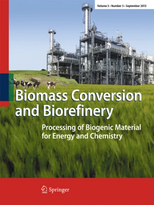
Figure 2 and Table 3 display the FTIR spectra of the PF, OL, and WS samples together with their functional groups. First, bands between 3000 and 3500 ${\mathrm{cm}}^{-1}$ that were attributed to OH stretching vibration confirmed the existence of water, protein, alcohol, and contaminants that were aromatic, phenolic, acidic, and water-soluble [8, 68]. For hydroxyl groups, this zone is specified in accordance with a specific frequency value, such as the indicated maximum of 3351.6 ${\mathrm{cm}}^{-1}$. Methylene, methoxyl C-H, and methyl groups, which are components of hemicellulose, are related with symmetrical and non-symmetrical vibrations in the band range between 3000 and 2700 ${\mathrm{cm}}^{-1}$ [69]. Gases like CO₂ and CO are present in the region between 2133 and 2000 ${\mathrm{cm}}^{-1}$. C≡C stretching of alkyne groups like ethene, propyne, 1-butyne, and 1-hexyne is accountable for a band of 2133 ${\mathrm{cm}}^{-1}$. The bands between 1627.63 and 1650.77 ${cm}^{-1}$ had attributed to a C–C stretch in ethers or aromatic compounds. The presence of cellulose, lignin, and protein in biomass was suggested by the band at 1500 ${\mathrm{cm}}^{-1}$ that was associated with a C = C aromatic ring [70, 71]. It is significant to note that the C–C bonds found in the lignin’s aromatic ring match the wavelength of 1510 ${\mathrm{cm}}^{-1}$ [72, 73]. Symmetric-antisymmetric glycosidic link C–O–C, ring C–C, C–O stretching, –OH, and –CH₂ bending vibrations, and C–H, CH₃ bend alkyl-chain structure CH₂, CH₃ deformation vibrations that indicate the existence of hemicellulose, cellulose, alkanes, or aliphatic skeletal (saturated hydrocarbon) compounds such as ethane, pentane, etc. are accountable for bands in the range of 1159 to 1444.5 ${\mathrm{cm}}^{-1}$. Aliphatic skeletal C–C, C–O–C, and C–OH stretching, as well as C–H bending vibrations, C–C, C–O stretching, and –OH bending vibrations, were also attributed to bands ranging from 778.136 to 1106 ${\mathrm{cm}}^{-1}$ that revealed the presence of esters characteristic of hemicellulose, cellulose, and amorphous cellulose as well as aliphatic compounds (saturated), joined by single bonds (alkynes). The bands between 610 and 467 ${\mathrm{cm}}^{-1}$ are attributed to substances such as alcohol, disulfides, R2S2 (C–S and S–S stretch), bending vibration of Si–O–Si and Si–O–, or stretching vibration of organic sulphur (aromatic double sulfide–S–S– or –SH) such as CH₃–CH₂–S–CH₃ 2-butyl 1-propyl sulphide, ethyl methyl sulphide, ethyl phenyl sulphide, etc. It was determined from the FTIR results that all samples are suitable feedstocks for pyrolysis. It is clear from looking at all the spectra that the determined region between 469 and 1650 ${\mathrm{cm}}^{-1}$ contains a concentration of peaks that stand out. These peaks correlate to some bands that stretch and deform into different vibrational groups and values, which are representative of the components of the lignocellulosic material. This range is extremely important for understanding changes (stretching and deformation vibrations) in the components of cellulose, hemicellulose, and lignin in lignocellulosic materials [74].

Fig. 2

FTIR spectra of palm fronds (PF), olive leaves (OL), and wheat straw (WS) samples

Table 3 Assignment of FTIR absorption bands for biomass materials

3.3 Scanning electron microscope analysis

Scanning electron microscopy (SEM) was used to examine the structure of biomass sample. SEM works well for describing the surface morphology of biomass [75]. This technique aids in examining any pores or anomalies that may be present on the sample surface. Figure 3 displays the outcomes of the study at various magnifications, and Table 4 displays the descriptive parameters derived from the photos using Image J analysis. As seen in Fig. 3, the surfaces of all samples had some regular, long, flat, and fibrous flakes. The explanation for why the surface morphology of all samples is nearly uniform is because there are a number of grains of comparable sizes as well as a few larger grains. No pores of any shape or size have been visible on the surface in the photos. Compared to the PF and OL samples, the WS particles appear significantly more elongated, and their distribution is more dispersed. By displaying how smaller particles cling to the surface of larger ones, the image effectively illustrates the agglomeration phenomenon.

Fig. 3

Scanning electron microscope (SEM) for different biomass materials

Table 4 Descriptive parameters obtained from SEM images based on Image J analysis

3.4 TG/DTG thermal degradation profiles

Figure 4 displays the TG/DTG and DTA profiles for the PF, OL, and WS samples during pyrolysis at heating rates of 10, 20, and 30 $^\circ{\rm C} /min$ regarding temperature and mass loss. The profiles demonstrate how various lignocellulosic materials typically behave during pyrolysis as well as how heating rate and material type affect behaviour. It is evident that for each heating rate in all profiles, the mass loss of the biomass samples rises with temperature. The pyrolysis process is a multistage decomposition of lignocellulosic biomass that can be divided into three phases based on their profiles: in the first stage, moisture is evaporated, and volatile CO and CO₂ are released. The temperature ranges in this drying stage for PF, OL, and WS for all ($\beta$) are (40–154 $^\circ{\rm C}$), (24–170 $^\circ{\rm C}$), and (30–160 $^\circ{\rm C}$), respectively. The mass losses at this stage are (7–7.5%) for PF, (6.3–6.7%) for OL, and (6.5–7.15) for WS, and they are well-matched to the results of proximate analysis. The second stage is the devolatilization or active pyrolytic stage, which occurs at (123–568 $^\circ{\rm C}$) for PF, (121–560 $^\circ{\rm C}$) for OL, and (114–525 $^\circ{\rm C}$) for WS for all ($\beta$), with the exception of WS at = 30 $^\circ{\rm C} /\mathrm{min}$, where this stage of devolatilization extended to 900 $^\circ{\rm C}$ where the mass loss rate increases violently as shown in Fig. 4. High molecular weight molecules were decomposed into lower molecular weight ones at this stage. In this stage, hemicellulose degradation (200–350 $^\circ{\rm C}$), lignin and cellulose decomposition (350–480 $^\circ{\rm C}$), and char formation zone of lignin degradation (> 480 $^\circ{\rm C}$) all take place [12]. Other sources state that cellulose decomposes between 230 and 450 $^\circ{\rm C}$, hemicellulose decomposes between 180 and 340 $^\circ{\rm C}$, while lignin undergoes thermal decomposition at temperatures over 500 $^\circ{\rm C}$ [76, 77]. At a greater temperature, liquid formation takes place because, at a lower temperature, cellulose first decomposes into monomers and produces CO, CO₂, and carbonaceous gases.

Fig. 4

TG/DTG and DTA of the biomass materials

In contrast, lignin decomposes more slowly and at temperatures exceeding 500 $^\circ{\rm C}$ as a result of its linkage with a hydroxyl phenolic group (see Table 3). For all biomass samples, the stage where complex compounds are decomposed into linear compounds by the constant flow of energy is the one with the highest rate of volatilization [39, 78, 79]. The majority of the volatiles were released at this time, and the secondary gas evolution was essentially finished, which encouraged the creation of carbon [80]. The majority of the cellulose, hemicellulose, and some lignin are said to be degrading at this stage, which results in a mass loss of (86.5–88.5%) for PF, (81.2–82.9%) for OL, and (81.3–84.7%) for WS. There is no degradation in the third zone of (530–1000 $^\circ{\rm C}$) for PF, (510–1000 $^\circ{\rm C}$) for OL, and (525–1000 $^\circ{\rm C}$) for WS for all ($\beta$), but the carbon and ashes are still included in the final solid waste. The lengthy tail at this stage represents lignin decomposition and char production, where the lignin has been converted more slowly in order to maximise carbonization. Lignin is covalently bonded to hemicellulose and cross-linked to polysaccharides; it is formed between cellulose and microfibers. The greater lignin content of OL caused the separation of hemicellulose and cellulose in addition to slowing down the rate of pyrolysis.

A significant factor affecting the yields of products like bio-oil, biochar, and non-condensable gases is the heating rate ($\beta$) in pyrolysis processes. Additionally, evaluating the kinetic and thermodynamic characteristics depends on it. The DTG curve showed three separate peaks for all biomass samples, with each peak shifting to a higher temperature with an increase in heating rate. The lower $\beta$ gave enough time for thermochemical reactions to cause the internal and external surfaces of the biomass samples to gather at the same temperature at a given time, which enabled its surface and interior to be decomposed simultaneously because biomass waste does not conduct heat well [81]. On the other hand, the slower reactions and the migration of the DTG profiles to higher temperature regions were caused by the greater heating rates' inability to elevate the internal temperature high enough to achieve the decomposition temperature [82,83,84]. The leftover solid materials (char) after pyrolysis also vary slightly with the heating rate. It is crucial to understand that strong heat flows during the final stage of heating (devolatilization) reduce the viscosity of the biomass material while accelerating the processes that produce volatiles. Several biofuels have shown this behaviour in the past [85, 86]. Two peaks are observed in the reactive stage that are evidence of hemicellulose and cellulose decomposition, while there is no indication of any peak derived from lignin decomposition, as shown in ref. [87]. On the other hand, the first peak is seen as a result of the first stage's elimination of moisture and light volatile materials. It can be seen from the comparison of the peaks of hemicellulose and cellulose in all samples that they have distinct shapes and locations, which suggests that the distribution of organic and inorganic chemicals has an impact on how quickly they degrade thermally. The maximum peak in the (DTG) profiles is where the greatest mass loss occurs, and the height of this maximum peak establishes the reactivity of the biomass materials. For PF, OL, and WS, respectively, the mass losses at the maximum peak are (44.5–47.5%), (33.–35.3%), and (38.5–45.25%) (see Table 5).

Table 5 Thermal degradation parameters for different biomass materials

3.5 Pyrolysis characterization of waste biomass materials

The order of the materials' increasing reactivity, as indicated by the DTG profiles of the three biomass samples, is PF > WS > OL, as shown in Table 5. The table also demonstrates that for all samples, the temperature at the greatest peak rises as $\beta$ rises while the time to reach it falls substantially. As demonstrated in Table 5, the rate of pyrolysis (${-R}_{p}$) increases as $\beta$ increases in the following order: WS > PF > OL. A greater $\beta$ was conducive to the pyrolysis, as evidenced by the rise in the maximum volatile release rate (${-R}_{p}$) or the maximum rate of the pyrolysis process with an increased $\beta$. ${R}_{p}$ increased as the rate was increased from 10 to 30 $^\circ{\rm C} /\mathrm{min}$ because there wasn’t enough time for the products to volatilize, causing the thermal hysteresis phenomenon [49]. Table 5 displays the pyrolysis characteristics and the samples' reactivity through the devolatilization and char stages (a, b). The reactivity index measures the rate of structural component deterioration as revealed by peak DTG profiles ($RM$). The results indicated that while PF and WS were the most reactive biomass samples, OL was least reactive at the volatile decomposition (reactive) stage. This is because the lignin composition of the OL exceeds that of its hemicellulose and cellulose constituents (see Table 1). On the other hand, at the char pyrolysis stage, PF became the most reactive. These are once more shown by the height of their DTG profiles within the two stages, as seen in Fig. 4. The residual mass ranges for PF, OL, and WS were (1.43–2.74%), (1.97–2.94%), and (1.11–3.67%), respectively, at the end of the experiment (1000 $^\circ{\rm C}$). These values resembled the ash contents for PF and WS in Table 1 considerably, demonstrating that the reaction was finished. Thermal hysteresis was primarily responsible for the variation in residual mass with varying heating rates.

Because the sample’s mass and heat transfers were hindered, some of the product's components didn't have enough time to volatilize, and thermal hysteresis occurred under the maximal pyrolysis rate, there was a proportional increase in (${T}_{p}$) with the ($\beta$) [32]. The results of Table 6 show that the ${D}_{dev}$ indices of the PF and WS samples were greater than those of the OL samples due to the latter's higher ${T}_{i}$ and ${T}_{p}$ and lower (${-R}_{p}$) than those of the other samples. The ${D}_{dev}$ index increases as $\beta$ increases for all samples. This demonstrates the benefit of high $\beta$ for devolatilizing biomass products. Indicating that the pyrolysis benefited from the quicker heating rate and that the volatiles was released more readily, $CPI$ increased as $\beta$ increased, but that there was not enough time for all of the volatiles to be released. The $CPI$ is increased for all samples in the following order: PF > OL > WS. Volatiles were liberated more quickly because PF and WS biomass samples had better pyrolysis properties and stability (higher $CPI$ and ${R}_{W}$). The acquired $CPI$ and ${R}_{W}$ values for each sample make this clear.

Table 6 Pyrolysis parameters for different materials

3.6 Chemical kinetics

3.6.1 Kinetics from integral models

In this method, the devolatilization process was taken as one zone for all samples, as shown in Table 7. All the data obtained using different diffusion and reaction order models are fitted, and the best-fit regression line that has the highest value of the correlation coefficient ${R}^{2}$ was determined, as shown in Fig. 5. Table 7 shows the values of $E$ and $A$ for all samples using different diffusion and reaction models at different heating rates ($\beta$). The values of ($E$) for the PF sample ranged between 30.36 and 167.13 $kJ/\mathrm{mole}$, 23.59 and 142.41 $kJ/\mathrm{mole}$, and 8.82 and 90.02 $kJ/\mathrm{mole}$ for diffusion models at β of 10, 20, and 30 $^\circ{\rm C} /\mathrm{min}$, respectively. On the other hand, for the PF sample, the values of ($E$) ranged between 66.49 and 117.49 $kJ/\mathrm{mole}$, 53.36 and 107.61 $kJ/\mathrm{mole}$, and 22.3 and 93.62 $kJ/\mathrm{mole}$ for β of 10, 20, and 30 $^\circ{\rm C} /\mathrm{min}$, respectively, for reaction order models. For the OL sample, the values of ($E$) ranged between 27.55 and 149.20 $kJ/\mathrm{mole}$, 23.06 and 131.69 $kJ/\mathrm{mole}$, and 23.29 and 130.51 $kJ/\mathrm{mole}$ for $\beta$ of 10, 20, and 30 $^\circ{\rm C} /\mathrm{min}$, respectively, for diffusion models. For reaction order models, the values of ($E$) ranged between 60.91 and 92.88 $kJ/\mathrm{mole}$, 52.0 and 83.41 $kJ/\mathrm{mole}$, and 51.69 and 83.18 $kJ/\mathrm{mole}$ at $\beta$ of 10, 20, and 30 $^\circ{\rm C} /\mathrm{min}$, respectively. For the WS sample, the values of ($E$) ranged between 25.04 and 149.92 $kJ/\mathrm{mole}$, 26.43 and 156.27 $kJ/\mathrm{mole}$, and 11.01 and 102.51 $kJ/\mathrm{mole}$ for $\beta$ of 10, 20, and 30 $^\circ{\rm C} /\mathrm{min}$, respectively, for diffusion models. For reaction order models with $\beta$ of 10, 20, and 30 $^\circ{\rm C} /\mathrm{min}$, $E$ values ranged from 56.87 to 117.38 $kJ/\mathrm{mole}$, 58.33 to 119.76 $kJ/\mathrm{mole}$, and 23.48 to 125.97 $kJ/\mathrm{mole}$, respectively. These results clarified that the ($\beta$) has an effect on the values of the ($E$). It can be seen that some diffusion–reaction models gave reasonable values of ($E$), which matched with other biomass materials in the literature. The diffusion models gave logical values (high values mean a fast and easy pyrolysis process) for ($A$), as shown in Table 7 compared to the reaction order models (low values). It can be seen that ${R}^{2}$ values showed low correlation values, especially for the diffusion models.

Table 7 Kinetic parameters of the biomass materials pyrolysis using an integral method based on different diffusion and reaction order models

Fig. 5

Fitting curves of the integral method for estimating the kinetic parameters of biomass pyrolysis based on different diffusion and reaction order models

3.6.2 Kinetics from isoconversional models

Figure 6 shows ($E$) and ($A$) distribution as $f(\mathrm{\alpha })$ using OFW, KAS, diffusion, and reaction order models, respectively. The OFW and KAS methods are used to estimate the activation energy, ($E$), at a specific extent of conversion (α) for an independent model. We can obtain the profile of the ($E$) as a function of (α) by repeating this procedure at different conversion values (α). The underlying assumption is that the reaction model $f(\mathrm{\alpha })$, is identical at a given (α) for a given reaction under different conditions. The frequency factor ($A$) was obtained from the intersection term of Eqs. 11 and 12 based on the values of the integral function $\mathrm{g}\left(\mathrm{\alpha }\right)$ in Eq. 6 and the estimated ($E$). Different algebraic functions of $\mathrm{g}\left(\mathrm{\alpha }\right)$ and $f(\mathrm{\alpha })$ that describe the reaction models are given in Table 2. The diffusion and reaction order models were used for estimating the frequency factor ($A$) based on the ($E$) values obtained from the OFW and KAS models for PF, OL, and WS biomass samples. The values of ${E}_{av}$ calculated by using OFW are 69.1, 91.9, and 65.2 $kJ/\mathrm{mole}$ for OL, PF, and WS samples, respectively, and ${E}_{av}$ calculated by using KAS is 101.8, 87.5, and 63.4 $kJ/\mathrm{mole}$ for OL, PF, and WS samples, respectively. The ${E}_{av}$ estimated using the OFW method was a little higher than the obtained values from KAS for the PF and WS biomass samples. The KAS, on the other hand, yields a higher value of ${E}_{av}$ than the value obtained from the KAS for the OL sample. The decomposition of hemicellulose and cellulose occurred mostly in the (α) range of 0.1–0.7, while lignin decomposed in the same range at the same time for OL and WS samples using both kinetic models. For (α > 0.7), there is a fluctuation in the values of ($E$) for the PF sample. The $E$ distribution showed a bell-shaped pattern with an increased (α) in the devolatilization temperature range of all samples (150–600 $^\circ{\rm C}$). The $E$ of the hemicellulose decomposition at the lower part of (α) was lower than that of the cellulose decomposition at the higher part of (α) in the range of 0.1–0.7 according to the two peaks in the DTG profiles in Fig. 4 and ref. [54]. The difference in the ${E}_{av}$ value between the OFW and KSA methods was 1.8, 4.4, and − 33.7 $kJ/\mathrm{mole}$ for PF, WS, and OL, respectively. When hemicellulose was decomposed to a certain extent (α > 0.25), the $E$ value began to increase, causing the decomposition of hemicellulose to overcome a higher energy barrier [88, 89]. When α > 0.7, the main reactant became lignin, which in turn led to a sharp decrease in $E$ for the WS and OL samples or a fluctuation between decrease and increase for the PF sample, which is opposed to that in ref. [90]. This is due to the difference in nature, composition, physical and chemical properties, etc. of the samples used in this study. The KAS and OFW models provide an efficient way to estimate activation energy [91], but the OFW method gives more reasonable values of ${E}_{av}$ than the KAS gave.

Fig. 6

Activation energy distribution using the OFW and KAS methods and the frequency factors obtained from OFW data for different diffusion and reaction order models

The pre-exponential factor ($A$) represents the number of collisions per time unit between atoms, which indicates the proper orientation for a reaction to take place. The value of $A$ increased with the increase in (α), which indicated the reliability of the calculated activation energy values. Figure 6 shows the distributions of $A$ as a function of (α) profiles using the $E$ values produced by the OFW method. Based on the ${E}_{\mathrm{\alpha }}$ values obtained using the OFW method, it can be seen that for reaction models, the distributions of $A$ are almost normal in the range of α = 0.3–0.7. The F0-reaction order model gives the lowest maximum $A$ value ($1.00\times {10}^{9} {\mathrm{min}}^{-1}$) and the F4-reaction order model gives the highest maximum value ($3.75\times {10}^{9} {\mathrm{min}}^{-1}$) for the OL sample. On the other hand, the distributions of $A$ for PF and WS samples are skewed to the right in the narrow range of α = 0.5–0.7 and PF shows very small peaks at α = 0.8 with peak values ranging between $0.25\times {10}^{10}$ and $2.50\times {10}^{10} {\mathrm{min}}^{-1}$ for PF, where fast pyrolysis in a short time has occurred, and $0.25\times {10}^{9}$ and $3.50\times {10}^{9} {\mathrm{min}}^{-1}$ for WS samples. For D2a and D2b diffusion models, the $A$ distribution for an OL sample is nearly normal in the range of = 0.3–0.7, with peak values ranging between $0.25\times {10}^{9}$ and $1.00\times {10}^{9} {\mathrm{min}}^{-1}$, respectively. On the other hand, the PF sample showed an uneven distribution of $A$ with a maximum peak value of $3.25\times {10}^{9} {\mathrm{min}}^{-1}$, but for WS, the distribution of $A$ skewed to the right with a maximum peak value of $3.25\times {10}^{8} {\mathrm{min}}^{-1}$ for the D2b model, as shown in Fig. 6. In general, reaction order models give higher $A$ values at the same range of (α), which shows that pyrolysis is easier and faster. The distributions of $A$ for all samples using the $E$ values from the KAS method for both diffusion and reaction models are almost the same, but with such small values of $A$, which means that the pyrolysis process is difficult and takes a long time for thermal degradation (see supplementary). In general, in the ranges of α $\le$ 0.2 and $\mathrm{\alpha }\ge$ 0.7, the degradation reactions may be different. Consequently, the isoconversional models indicated variations in both ${E}_{\mathrm{\alpha }}$ and ${A}_{\mathrm{\alpha }}$ values, with an increase in the conversion degree (α). This observation provides evidence that the degradation process for these samples takes place in multiple steps. Average activation energy values obtained from the integral method based on the diffusion integral models are to some extent similar to those obtained from the KAS method, as highlighted in Table 7. Whereas the average activation energy values obtained based on the reaction order integral models are similar to those obtained from the OFW method, as also highlighted in Table 7.

3.6.3 Kinetics from DTA model

Figure 4a shows the DTA profiles of the biomass samples (PF, OL, and WS) at 10, 20, and 30 $^\circ{\rm C} /\mathrm{min}$. For all $\beta$ values, the DTA profiles are divided into three zones, where an exothermic effect is registered. For all $\beta$ values; the first, second, and third zones lie between 85 and 238 $^\circ{\rm C}$, 236 and 399 $^\circ{\rm C}$, and 387 and 582 for PF, respectively; lie between 86–224 $^\circ{\rm C}$, 223–432 $^\circ{\rm C}$, and 396–576 $^\circ{\rm C}$ for OL, respectively; and lie between 84 and 270 $^\circ{\rm C}$, 233 and 403 $^\circ{\rm C}$, and 391 and 553 $^\circ{\rm C}$ for WS, respectively. The samples dried, and the hemicellulose decomposed with one peak in the first zone for all samples except that at β = 30 $^\circ{\rm C} /\mathrm{min}$, PF and OL did not show any peaks. The peak temperatures in this zone ranged between 140 and 176 $^\circ{\rm C}$, 133 and 194 $^\circ{\rm C}$, and 136 and 213 $^\circ{\rm C}$ for PF, OL, and WS, respectively. The second thermal zone demonstrated an exothermic effect where the cellulose decomposed, with one high peak, especially at $\beta$ = 30 $^\circ{\rm C} /\mathrm{min}$, and two small peaks at other values of $\beta$ for all samples. The peak temperatures in this zone range between 306 and 340 $^\circ{\rm C}$, 330 and 361 $^\circ{\rm C}$, and 306 and 353 $^\circ{\rm C}$ for PF, OL, and WS, respectively. The third zone showed an exothermic effect, with almost the highest peak at $\beta$ =20 $^\circ{\rm C} /\mathrm{min}$ for WS and at $\beta$ =30 $^\circ{\rm C} /\mathrm{min}$ for PF and OL samples, and two small peaks at other values of $\beta$ for all samples. The peak temperatures ranged between 432 and 461 $^\circ{\rm C}$, 473 and 499 $^\circ{\rm C}$, and 441 and 456 $^\circ{\rm C}$ for PF, LO, and WS, respectively. The zone characteristic parameters are shown in Table 8. The activation energy ($E$) of all biomass samples was calculated using the direct method using Eq. (13) and the fitting method using Eq. (14), with the coefficients determined from the experimental function $1/{T}_{max}=f(\mathrm{ln})$. The $E$ values calculated from DTA measurements for all samples are given in Table 8. The table, to some extent, is in agreement with some of the data obtained by integral methods for diffusion and reaction order models. The ${E}_{av}$ values from DTA using the fit method are 131.46, 175.32, and 47.8 $kJ/\mathrm{mole}$. Except for the ${E}_{av}$ value for WS, these results are much higher than those produced using the OFW and KAS approaches. On the other hand, the ${E}_{av}$ value of WS is lower than those produced using the OFW and KAS methods. Since the direct method depends on ${T}_{in}$, which is so small compared to ${T}_{max}$, which is used in the fit method, the produced ${E}_{av}$ values are underestimated.

Table 8 DTA transition characteristics and kinetic parameters of the biomass materials

3.7 Thermodynamic parameters

Using diffusion and reaction order models and the $E$ values derived from the OFW and KAS models in the range of α = 0.2–0.8, the estimated thermodynamic parameters ${\Delta \mathrm{H}}_{av}$, ${\Delta \mathrm{G}}_{av}$, and ${\Delta \mathrm{S}}_{av}$ are illustrated in Fig. 7a, b. The $\Delta \mathrm{H}$ is the amount of energy needed to break down the complex chemical bonds in waste biomass and form new ones; it also indicates whether an action is endothermic or exothermic. A positive ∆H value also suggests that the thermal degradation reactions are all endothermic since energy is needed for the reactants to reach their transition state [92]. The value of $\Delta \mathrm{H}$ increases with (α), as seen in Fig. 7a, b, except for WS, which exhibits a decline in $\Delta \mathrm{H}$ for α > 0.7. Based on the $E$ from the KAS model and the $A$ from the diffusion and reaction order models, the ${\Delta \mathrm{H}}_{av}$ of PF, OL, and WS are 88, 105, and 62 $kJ/\mathrm{mole}$ respectively, and for the OFW model, they are 88, 105, and 62 $kJ/\mathrm{mole}$. This indicates that additional heat energies are needed for the OL decomposition process, PF, and WS to break the reagent bonds, which is consistent with the $E$ value obtained from the OFW model but not with the $E$ value obtained from the KAS model. The difference in potential energy barrier between ${E}_{av}$ and ${\Delta \mathrm{H}}_{av}$ was only 3.9, 36.9, and 3.2 $kJ/\mathrm{mole}$ for the OFW, and 4.6, 29.8, and 5.5 $kJ/\mathrm{mole}$ for the KAS for the PF and WS samples, respectively. This revealed that the reaction was viable under the conditions that were present. The favourable formation of the activation complex is indicated by the little amount of energy used during the thermochemical conversion of materials to produce various products, such as liquid, gas, and biochar, as well as by the slight difference between ${E}_{av}$ and ${\Delta \mathrm{H}}_{av}$ for PF and WS samples [93].

Fig. 7

a Thermodynamics parameters for the biomass materials based on the kinetics from the OFW model and frequency factor from the diffusion and reaction order models. b Thermodynamics parameters for the biomass materials based on the kinetics from the KAS model and frequency factor from the diffusion and reaction order models

The $\Delta \mathrm{G}$ reveals that the total energy increase of the system occurs with the approach of the reagents and the formation of the activated complex [94]. It indicates that high energy can be evolved from the biomass samples. Figure 7a, b shows that $\Delta \mathrm{G}$ is nearly fixed in the range of α = 0.2–0.7 for PF and WS samples, then it fluctuates up and down up to α = 0.8 for all diffusion and reaction order models used. The OL sample, on the other hand, exhibits this behaviour only when the OFW model is used as a source of $E$, whereas for the KAS model, the $\Delta \mathrm{G}$ values increase as (α) increases up to 0.7, then decay until it reaches α = 0.8 for all diffusion and reaction order models used. For diffusion models, the (${\Delta \mathrm{G}}_{av}$) values calculated by the OFW model are 185, 181, and 184 $kJ/\mathrm{mole}$ for PF, OL, and WS samples, respectively, and for reaction order models, they are 171, 167, and 170 $kJ/\mathrm{mole}$ for PF, OL, and WS, respectively. For diffusion models, the ${\Delta \mathrm{G}}_{av}$ values calculated by the KAS model are 187, 191, and 190 $kJ/\mathrm{mole}$ for PF, OL, and WS samples, respectively, and 173, 177, and 176 $kJ/\mathrm{mole}$ for PF, OL, and WS, respectively, for reaction order models. There are small differences between the ${\Delta \mathrm{G}}_{av}$ calculated by OFW and KAS using diffusion and reaction order models (2–10 $kJ/mole$). The ${\Delta \mathrm{G}}_{av}$ values from 182 to 184 $kJ/\mathrm{mole}$ and 171 to 175 $kJ/\mathrm{mole}$ for different biomasses are reported in ref. [55]. During thermal degradation, the disorder change can be evaluated using $\Delta \mathrm{G}$, with low $\Delta \mathrm{G}$ values favouring the reaction [95]. According to these values, the suitability order of the degradation process was OL > WS > PF for OFW and KAS using diffusion and reaction order models. So, OL and WS consumed a great part of the heat in the decomposition process, disordering the system, and supporting the pyrolysis process.

The $\Delta \mathrm{S}$ had negative variation values with (α), indicating a lower degree of disorder in the products compared to the initial biomass in the thermal degradation process [96], as shown in Fig. 7a, b. At this condition, the material showed little reactivity, and it took more time to form an activated complex. On the other hand, the higher value of entropy implies that the material is too far from its own thermodynamic equilibrium, its reactivity is higher, and it takes less time to form the activated complex, which results in short reaction times [94]. The ${\Delta \mathrm{S}}_{av}$ values calculated by the OFW model according to the order of decreasing negative values are − 0.183, − 0.154, and − 0.192 kJ/K mole for OL, PF, and WS samples, respectively, for diffusion models, and are − 0.131, − 0.160, and − 0.169 kJ/K mole for PF, OL, and WS, respectively, for reaction order models. The ${\Delta \mathrm{S}}_{av}$ calculated by the KAS model are − 0.144, − 0.166, and − 0.212 kJ/K mole for OL, PF, and WS samples, respectively, for diffusion models, and − 0.120, − 0.143, and − 0.188 kJ/K mole for OL, PF, and WS, respectively, for reaction order models. The sign of ${\Delta \mathrm{G}}_{av}$ is positive at all temperatures, and the degradation process is never spontaneous since, in general, thermal decomposition is endothermic, ${\Delta \mathrm{H}}_{av}>0$, and the entropy of the system decreases, ${\Delta \mathrm{S}}_{av}<0$.

4 Conclusion

The key conclusions from the results of the present study are as follows:

• It was shown that three biomasses had a high deposition risk (${R}_{b/a}>1.0, Fu>40.0)$, related to fouling and slagging problems. However, FTIR data supported the findings that all samples are suitable feedstock for pyrolysis and yield products.

• As the heating rate increases, the rate of pyrolysis ($-{R}_{p}$) increases in the following order: WS > PF > OL. The fact that the maximum rate of the pyrolysis process ($-{R}_{p}$) increased with the heating rate suggesting that pyrolysis was facilitated by higher heating rates.

• For all samples, the ${D}_{dev}$ and $CPI$ indices rise as $\beta$ rises. For all samples, the $CPI$ is increased in the following order: PF > OL > WS. Since PF and WS biomass samples showed greater pyrolysis characteristics and stability (higher $CPI$ and ${R}_{W}$), volatiles were released more readily. This is evident from the obtained $CPI$ and ${R}_{W}$ values for all samples.

• The KAS and OFW models provide an efficient way to estimate activation energy. The values of ${E}_{av}$ calculated by using OFW are 69.1, 91.9, and 65.2 $kJ/\mathrm{mole}$ for OL, PF, and WS samples, respectively, and for KAS, are 101.8, 87.5, and 63.4 $kJ/\mathrm{mole}$ for OL, PF, and WS samples, respectively.

• Using the ($E$) values from the KAS technique for diffusion and reaction models, the distribution of ($A$) for all samples is almost same, but with such small values of ($A$), it suggests that the pyrolysis process is highly difficult and takes a very long time for thermal degradation of the materials.

• Average activation energies based on diffusion integral models and derived by the integral technique are quite comparable to those based on the KAS method. The average activation energy values obtained using the reaction order integral models, however, are comparable to those found using the OFW technique.

• The ${E}_{av}$ values from DTA using the fit method are 131.46, 175.32, and 47.8 $kJ/\mathrm{mole}$. With the exception of the ${E}_{av}$ value for WS, these results are much higher than those produced using the OFW and KAS approaches.

• The small energy consumption during the thermochemical conversion of materials to produce a variety of products like liquid, gas, and biochar is reproduced by the little difference between the ${E}_{av}$ and ${\Delta \mathrm{H}}_{av}$, and enthalpy was computed for the PF and WS samples.

• According to ${\Delta \mathrm{G}}_{av}$ values, the degradation process was appropriate for OFW and KAS in the following sequence: OL > WS > PF using diffusion and reaction order models. As a result, the thermal decomposition generated a substantial amount of heat, which OL and WS absorbed, disturbing the system and promoting pyrolysis.

• Using diffusion and reaction order models, the degradation process was suitable for OFW and KAS in the following order: OL > WS > PF, as indicated by ${\Delta \mathrm{H}}_{av}$ values. Therefore, OL and WS consumed a significant portion of the heat produced by the breakdown process, disorganizing the system and promoting pyrolysis.

• In general, the degradation process is never spontaneous since thermal decomposition is endothermic, ${\Delta \mathrm{H}}_{av}>0$, and the entropy of the system decreases, ${\Delta \mathrm{S}}_{av}<0$, and the sign of ΔG_av is positive at all temperatures.

References

Hameed Z, Naqvi SR, Naqvi M et al (2020) A comprehensive review on thermal coconversion of biomass, sludge, coal, and their blends using thermogravimetric analysis. J Chem 2020:5024369, 23 pages
Naqvi M, Yan J, Dahlquist E, Naqvi SR (2016) Waste biomass gasification based off-grid electricity generation: A case study in pakistan. Energy Proc 103:406–412. https://doi.org/10.1016/j.egypro.2016.11.307
Mostafa ME, He L, Xu J et al (2019) Investigating the effect of integrated CO2 and H2O on the reactivity and kinetics of biomass pellets oxy-steam combustion using new double parallel volumetric model (DVM). Energy 179:343–357. https://doi.org/10.1016/j.energy.2019.04.206
Naqvi M, Yan J, Dahlquist E, Naqvi SR (2017) Off-grid electricity generation using mixed biomass compost: a scenario-based study with sensitivity analysis. Appl Energy 201:363–370. https://doi.org/10.1016/j.apenergy.2017.02.005
Salman CA, Naqvi M, Thorin E, Yan J (2018) Gasification process integration with existing combined heat and power plants for polygeneration of dimethyl ether or methanol: a detailed profitability analysis. Appl Energy 226:116–128. https://doi.org/10.1016/j.apenergy.2018.05.069
Naqvi M, Dahlquist E, Yan J (2017) Complementing existing CHP plants using biomass for production of hydrogen and burning the residual gas in a CHP boiler. Biofuels 8:675–683. https://doi.org/10.1080/17597269.2016.1153362
Qureshi AS, Khushk I, Naqvi SR, et al (2017) Fruit waste to energy through open fermentation. Energy Proc 142:904–909. https://doi.org/10.1016/j.egypro.2017.12.145
Klass DL (1998) Chapter 2 - biomass as an energy resource: Concept and markets, biomass for renewable energy, fuels, and chemicals, academic press. Pages 29–50. https://doi.org/10.1016/B978-012410950-6/50004-0
Hu M, Chen Z, Wang S et al (2016) Thermogravimetric kinetics of lignocellulosic biomass slow pyrolysis using distributed activation energy model, Fraser-Suzuki deconvolution, and iso-conversional method. Energy Convers Manag 118:1–11
Naqvi SR, Naqvi M (2018) Catalytic fast pyrolysis of rice husk: influence of commercial and synthesized microporous zeolites on deoxygenation of biomass pyrolysis vapors. Int J Energy Res 42:1352–1362. https://doi.org/10.1002/er.3943
Nawaz A, Mishra RK, Sabbarwal S, Kumar P (2021) Studies of physicochemical characterization and pyrolysis behavior of low-value waste biomass using Thermogravimetric analyzer: evaluation of kinetic and thermodynamic parameters. Bioresour Technol Reports 16:100858. https://doi.org/10.1016/j.biteb.2021.100858
Boiko EA, Pachkovskii SV (2004) (2004) A kinetic model of thermochemical transformation of solid organic fuels. Russ J Appl Chem 779(77):1547–1555. https://doi.org/10.1007/S11167-005-0070-0
Olatunji OO, Akinlabi SA, Mashinini MP, Fatoba SO, Ajayi OO (2018) Thermo-gravimetric characterization of biomass properties: A review. In: IOP conference series: Materials Science and Engineering. p 012175. https://doi.org/10.1088/1757-899X/423/1/012175
Parthasarathy P, Narayanan KS, Arockiam L (2013) Study on kinetic parameters of different biomass samples using thermo-gravimetric analysis. Biomass Bioenerg 58:58–66. https://doi.org/10.1016/j.biombioe.2013.08.004
Castells B, Amez I, Medic L et al (2021) Study of lignocellulosic biomass ignition properties estimation from thermogravimetric analysis. J Loss Prev Process Ind 71:104425. https://doi.org/10.1016/j.jlp.2021.104425
Wiedemann H-G, Bayer G (2006) Trends and applications of thermogravimetry. In: Inorganic and Physical Chemistry. Topics in Current Chemistry, vol 77. Springer, Berlin, Heidelberg. https://doi.org/10.1007/BFb0048038
Yao X, Xu K, Liang Y (2017) Assessing the effects of different process parameters on the pyrolysis behaviors and Thermal Dynamics of corncob fractions. BioResources 12:2748–2767
Abbasi T, Abbasi SA (2010) Biomass energy and the environmental impacts associated with its production and utilization. Renew Sustain Energy Rev 14:919–937
Lédé J (2012) Cellulose pyrolysis kinetics: an historical review on the existence and role of intermediate active cellulose. J Anal Appl Pyrolysis 94:17–32
El-Sayed SA, Khairy M (2015) Effect of heating rate on the chemical kinetics of different biomass pyrolysis materials. Biofuels 6:157–170. https://doi.org/10.1080/17597269.2015.1065590
Ounas A, Aboulkas A, El harfi K et al (2011) Pyrolysis of olive residue and sugar cane bagasse: Non-isothermal thermogravimetric kinetic analysis. Bioresour Technol 102:11234–11238. https://doi.org/10.1016/j.biortech.2011.09.010
Wang C, Wang X, Jiang X et al (2019) The thermal behavior and kinetics of co-combustion between sewage sludge and wheat straw. Fuel Process Technol 189:1–14. https://doi.org/10.1016/j.fuproc.2019.02.024
Wang B, Li Y, Zhou J et al (2021) Thermogravimetric and kinetic analysis of high-temperature thermal conversion of pine wood sawdust under co2/ar. Energies 14:5328. https://doi.org/10.3390/en14175328
Romero Millán LM, Sierra Vargas FE, Nzihou A (2017) Kinetic analysis of tropical lignocellulosic agrowaste pyrolysis. Bioenergy Res 10:832–845. https://doi.org/10.1007/s12155-017-9844-5
Patidar K, Singathia A, Vashishtha M et al (2022) Investigation of kinetic and thermodynamic parameters approaches to non-isothermal pyrolysis of mustard stalk using model-free and master plots methods. Mater Sci Energy Technol 5:6–14. https://doi.org/10.1016/j.mset.2021.11.001
Ma Z, Chen D, Gu J et al (2015) Determination of pyrolysis characteristics and kinetics of palm kernel shell using TGA–FTIR and model-free integral methods. Energy Convers Manag 89:251–259. https://doi.org/10.1016/J.ENCONMAN.2014.09.074
Khalideh Al bkoor Alrawashdeh, Katarzyna Slopiecka, Abdullah A. Alshorman et al (2017) Pyrolytic degradation of Olive Waste Residue (OWR) by TGA: thermal decomposition behavior and kinetic study. J Energy Power Eng 11:497–510. https://doi.org/10.17265/1934-8975/2017.08.001
Mahmood H, Shakeel A, Abdullah A et al (2021) A comparative study on suitability of model-free and model-fitting kinetic methods to non-isothermal degradation of lignocellulosic materials. Polymers (Basel) 13:2504. https://doi.org/10.3390/polym13152504
Wang G, Zhang J, Shao J et al (2016) Thermal behavior and kinetic analysis of co-combustion of waste biomass/low rank coal blends. Energy Convers Manag 124:414–426
Gil MV, Riaza J, Álvarez L et al (2012) Kinetic models for the oxy-fuel combustion of coal and coal / biomass blend chars obtained in N2 and CO2 atmospheres. Energy 48:510–518
Amer M, Nour M, Ahmed M et al (2021) Kinetics and physical analyses for pyrolyzed Egyptian agricultural and woody biomasses: effect of microwave drying. Biomass Convers Biorefinery 11:2855–2868. https://doi.org/10.1007/s13399-020-00684-3
Huang J, Liu J, Chen J et al (2018) Combustion behaviors of spent mushroom substrate using TG-MS and TG-FTIR: thermal conversion, kinetic, thermodynamic and emission analyses. Bioresour Technol 266:389–397. https://doi.org/10.1016/J.BIORTECH.2018.06.106
Hu J, Yan Y, Evrendilek F et al (2019) Combustion behaviors of three bamboo residues: Gas emission, kinetic, reaction mechanism and optimization patterns. J Clean Prod 235:549–561. https://doi.org/10.1016/J.JCLEPRO.2019.06.324
Özsin G, Pütün AE (2019) TGA/MS/FT-IR study for kinetic evaluation and evolved gas analysis of a biomass/PVC co-pyrolysis process. Energy Convers Manag 182:143–153. https://doi.org/10.1016/j.enconman.2018.12.060
Zhang W, Zhang J, Ding Y et al (2021) Pyrolysis kinetics and reaction mechanism of expandable polystyrene by multiple kinetics methods. J Clean Prod 285:125042. https://doi.org/10.1016/j.jclepro.2020.125042
Alves JLF, da Silva JCG, da Silva Filho VF et al (2019) Kinetics and thermodynamics parameters evaluation of pyrolysis of invasive aquatic macrophytes to determine their bioenergy potentials. Biomass Bioenerg 121:28–40. https://doi.org/10.1016/J.BIOMBIOE.2018.12.015
Coats AW, Redfern JP (1965) Kinetic parameters from thermogravimetric data. II. J Polym Sci Part B Polym Lett 3:68–69. https://doi.org/10.1002/POL.1965.110031106
Açıkalın K (2022) Evaluation of orange and potato peels as an energy source: a comprehensive study on their pyrolysis characteristics and kinetics. Biomass Convers Biorefinery 12:501–514. https://doi.org/10.1007/S13399-021-01387-Z/TABLES/4
Mishra RK, Mohanty K (2018) Pyrolysis kinetics and thermal behavior of waste sawdust biomass using thermogravimetric analysis. Bioresour Technol 251:63–74. https://doi.org/10.1016/J.BIORTECH.2017.12.029
El-Sayed SA, Mostafa ME (2014) Pyrolysis characteristics and kinetic parameters determination of biomass fuel powders by differential thermal gravimetric analysis (TGA/DTG). Energy Convers Manag 85:165–172
Chen R, Li Q, Xu X, Zhang D (2019) Pyrolysis kinetics and reaction mechanism of representative non-charring polymer waste with micron particle size. Energy Convers Manag 198:111923. https://doi.org/10.1016/j.enconman.2019.111923
Lopes FCR, Tannous K, Rueda-Ordóñez YJ (2016) Combustion reaction kinetics of guarana seed residue applying isoconversional methods and consecutive reaction scheme. Bioresour Technol 219:392–402. https://doi.org/10.1016/j.biortech.2016.07.099
Ashraf A, Sattar H, Munir S (2019) A comparative applicability study of model-fitting and model-free kinetic analysis approaches to non-isothermal pyrolysis of coal and agricultural residues. Fuel 240:326–333. https://doi.org/10.1016/j.fuel.2018.11.149
Flynn JH (1997) The “temperature integral” - its use and abuse. Thermochim Acta 300:83–92. https://doi.org/10.1016/S0040-6031(97)00046-4
Ozawa T (1965) A new method of analyzing thermogravimetric data. Bull Chem Soc Jpn 38:1881–1886
Doyle CD (1962) Estimating isothermal life from thermogravimetric data. J Appl Polym Sci 6:639–642
Hu J, Song Y, Liu J et al (2020) Combustions of torrefaction-pretreated bamboo forest residues: physicochemical properties, evolved gases, and kinetic mechanisms. Bioresour Technol 304:122960. https://doi.org/10.1016/j.biortech.2020.122960
Boycheva S, Zgureva D, Vassilev V (2013) Kinetic and thermodynamic studies on the thermal behaviour of fly ash from lignite coals. Fuel 108:639–646. https://doi.org/10.1016/j.fuel.2013.02.042
Zhang J, Liu J, Evrendilek F et al (2019) TG-FTIR and Py-GC/MS analyses of pyrolysis behaviors and products of cattle manure in CO2 and N2 atmospheres: kinetic, thermodynamic, and machine-learning models. Energy Convers Manag 195:346–359. https://doi.org/10.1016/j.enconman.2019.05.019
Meng H, Wang S, Wu Z et al (2019) Thermochemical behavior and kinetic analysis during co-pyrolysis of starch biomass model compound and lignite. Energy Procedia 158:400–405. https://doi.org/10.1016/j.egypro.2019.01.123
El-Sayed SA, Mostafa ME (2020) Thermal pyrolysis and kinetic parameter determination of mango leaves using common and new proposed parallel kinetic models. RSC Adv 10:18160–18179. https://doi.org/10.1039/d0ra00493f
Alves JLF, Da Silva JCG, da Silva Filho VF et al (2019) Bioenergy potential of red macroalgae Gelidium floridanum by pyrolysis: evaluation of kinetic triplet and thermodynamics parameters. Bioresour Technol 291:121892. https://doi.org/10.1016/j.biortech.2019.121892
Edreis EMA, Li X, Atya AHA et al (2020) Kinetics, thermodynamics and synergistic effects analyses of petroleum coke and biomass wastes during H2O co-gasification. Int J Hydrogen Energy 45:24502–24517. https://doi.org/10.1016/j.ijhydene.2020.06.239
McKendry P (2002) Energy production from biomass (part 1): overview of biomass. Bioresour Technol 83:37–46. https://doi.org/10.1016/S0960-8524(01)00118-3
Ahmad MS, Mehmood MA, Al Ayed OS et al (2017) Kinetic analyses and pyrolytic behavior of Para grass (Urochloa mutica) for its bioenergy potential. Bioresour Technol 224:708–713. https://doi.org/10.1016/J.BIORTECH.2016.10.090
Chen J, Fan X, Jiang B et al (2015) Pyrolysis of oil-plant wastes in a TGA and a fixed-bed reactor: thermochemical behaviors, kinetics, and products characterization. Bioresour Technol 192:592–602. https://doi.org/10.1016/j.biortech.2015.05.108
Sait HH, Hussain A, Salema AA, Ani FN (2012) Pyrolysis and combustion kinetics of date palm biomass using thermogravimetric analysis. Bioresour Technol 118:382–389
Ríos-Badrán IM, Luzardo-Ocampo I, García-Trejo JF et al (2020) Production and characterization of fuel pellets from rice husk and wheat straw. Renew Energy 145:500–507. https://doi.org/10.1016/J.RENENE.2019.06.048
EL-Sayed SA, Mostafa ME (2021) Kinetics, thermodynamics, and combustion characteristics of Poinciana pods using TG/DTG/DTA techniques. Biomass Convers Biorefinery 1:1–25. https://doi.org/10.1007/S13399-021-02021-8/TABLES/8
Vassilev SV, Baxter D, Andersen LK, Vassileva CG (2010) An overview of the chemical composition of biomass. Fuel 89:913–933. https://doi.org/10.1016/J.FUEL.2009.10.022
Wauton I, Ogbeide SE (2022) Investigation of the production of pyrolytic bio-oil from water hyacinth (Eichhornia crassipes) in a fixed bed reactor using pyrolysis process. Biofuels 13:189–195. https://doi.org/10.1080/17597269.2019.1660061
Liu WJ, Tian K, Jiang H et al (2012) Selectively improving the bio-oil quality by catalytic fast pyrolysis of heavy-metal-polluted biomass: take copper (Cu) as an example. Environ Sci Technol 46:7849–7856. https://doi.org/10.1021/ES204681Y
Al Chami Z, Amer N, Smets K et al (2014) Evaluation of flash and slow pyrolysis applied on heavy metal contaminated Sorghum bicolor shoots resulting from phytoremediation. Biomass Bioenerg 63:268–279. https://doi.org/10.1016/J.BIOMBIOE.2014.02.027
Fang H, Huang L, Wang J et al (2016) Environmental assessment of heavy metal transport and transformation in the Hangzhou Bay, China. J Hazard Mater 302:447–457. https://doi.org/10.1016/j.jhazmat.2015.09.060
Dastyar W, Raheem A, He J, Zhao M (2019) Biofuel production using thermochemical conversion of heavy metal-contaminated biomass (HMCB) Harvested from Phytoextraction Process. Chem Eng J 358:759–785
Kovacs H, Szemmelveisz K, Koós T (2016) Theoretical and experimental metals flow calculations during biomass combustion. Fuel 185:524–531. https://doi.org/10.1016/j.fuel.2016.08.007
Shao J, Yan R, Chen H et al (2010) Catalytic effect of metal oxides on pyrolysis of sewage sludge. Fuel Process Technol 91:1113–1118. https://doi.org/10.1016/J.FUPROC.2010.03.023
Doshi P, Srivastava G, Pathak G, Dikshit M (2014) Physicochemical and thermal characterization of nonedible oilseed residual waste as sustainable solid biofuel. Waste Manag 34:1836–1846. https://doi.org/10.1016/j.wasman.2013.12.018
Popescu CM, Popescu MC, Vasile C (2011) Structural analysis of photodegraded lime wood by means of FT-IR and 2D IR correlation spectroscopy. Int J Biol Macromol 48:667–675. https://doi.org/10.1016/J.IJBIOMAC.2011.02.009
Chintala V, Kumar S, Pandey JK et al (2017) Solar thermal pyrolysis of non-edible seeds to biofuels and their feasibility assessment. Energy Convers Manag 153:482–492. https://doi.org/10.1016/j.enconman.2017.10.029
Sharma RK, Wooten JB, Baliga VL et al (2004) Characterization of chars from pyrolysis of lignin. Fuel 83:1469–1482. https://doi.org/10.1016/j.fuel.2003.11.015
Xu C, Etcheverry T (2008) Hydro-liquefaction of woody biomass in sub- and super-critical ethanol with iron-based catalysts. Fuel 87:335–345. https://doi.org/10.1016/J.FUEL.2007.05.013
Kim JY, Hwang H, Oh S et al (2014) Investigation of structural modification and thermal characteristics of lignin after heat treatment. Int J Biol Macromol 66:57–65. https://doi.org/10.1016/J.IJBIOMAC.2014.02.013
Baeza J (2001) Freer J Chemical characterization of wood and its components. In: Hon D-S, Shiraishi N (eds.) Wood and Cellulosic Chemistry, Chapter 8. Marcel Dekker Inc., New York, NY, USA. pp. 275–384
Claoston N, Samsuri AW, Ahmad Husni MH, Mohd Amran MS (2014) Effects of pyrolysis temperature on the physicochemical properties of empty fruit bunch and rice husk biochars. Waste Manag Res 32:331–339. https://doi.org/10.1177/0734242X14525822
Lyon RE (1997) An integral method of nonisothermal kinetic analysis. Thermochim Acta 297:117–124. https://doi.org/10.1016/S0040-6031(97)00158-5
Du Z, Sarofim AF, Longwell JP (1990) Activation energy distribution in temperature-programmed desorption: modeling and application to the soot–oxygen system. Energy Fuels 4:296–302. https://doi.org/10.1021/EF00021A014/ASSET/EF00021A014.FP.PNG_V03
Uçar S, Karagöz S (2009) The slow pyrolysis of pomegranate seeds: the effect of temperature on the product yields and bio-oil properties. J Anal Appl Pyrolysis 84:151–156. https://doi.org/10.1016/J.JAAP.2009.01.005
Pradhan D, Singh RK, Bendu H, Mund R (2016) Pyrolysis of Mahua seed (Madhuca indica) - production of biofuel and its characterization. Energy Convers Manag 108:529–538. https://doi.org/10.1016/j.enconman.2015.11.042
Vamvuka D, Kakaras E, Kastanaki E, Grammelis P (2003) Pyrolysis characteristics and kinetics of biomass residuals mixtures with lignite☆. Fuel 82:1949–1960. https://doi.org/10.1016/S0016-2361(03)00153-4
Cai H, Liu J, Xie W et al (2019) Pyrolytic kinetics, reaction mechanisms and products of waste tea via TG-FTIR and Py-GC/MS. Energy Convers Manag 184:436–447. https://doi.org/10.1016/J.ENCONMAN.2019.01.031
Quan C, Li A, Gao N (2009) Thermogravimetric analysis and kinetic study on large particles of printed circuit board wastes. Waste Manag 29:2353–2360. https://doi.org/10.1016/J.WASMAN.2009.03.020
Kumar A, Wang L, Dzenis YA et al (2008) Thermogravimetric characterization of corn stover as gasification and pyrolysis feedstock. Biomass Bioenerg 32:460–467. https://doi.org/10.1016/J.BIOMBIOE.2007.11.004
Wang G, Li W, Li B, Chen H (2008) TG study on pyrolysis of biomass and its three components under syngas. Fuel 87:552–558. https://doi.org/10.1016/J.FUEL.2007.02.032
Meesri C, Moghtaderi B (2002) Lack of synergetic effects in the pyrolytic characteristics of woody biomass/coal blends under low and high heating rate regimes. Biomass Bioenerg 23:55–66. https://doi.org/10.1016/S0961-9534(02)00034-X
Jeguirim M, Trouvé G (2009) Pyrolysis characteristics and kinetics of Arundo donax using thermogravimetric analysis. Bioresour Technol 100:4026–4031. https://doi.org/10.1016/J.BIORTECH.2009.03.033
Gašparovič L, Koreňová Z (2009) Jelemenský Ľ (2009) Kinetic study of wood chips decomposition by TGA. Chem Pap 642(64):174–181. https://doi.org/10.2478/S11696-009-0109-4
Lopez-Velazquez MA, Santes V, Balmaseda J, Torres-Garcia E (2013) Pyrolysis of orange waste: a thermo-kinetic study. J Anal Appl Pyrolysis 99:170–177. https://doi.org/10.1016/J.JAAP.2012.09.016
Chen D, Cen K, Zhuang X et al (2022) Insight into biomass pyrolysis mechanism based on cellulose, hemicellulose, and lignin: evolution of volatiles and kinetics, elucidation of reaction pathways, and characterization of gas, biochar and bio‐oil. Combust Flame 242:112142. https://doi.org/10.1016/j.combustflame.2022.112142
Chen D, Zheng Y, Zhu X (2013) In-depth investigation on the pyrolysis kinetics of raw biomass. Part I: Kinetic analysis for the drying and devolatilization stages. Bioresour Technol 131:40–46. https://doi.org/10.1016/j.biortech.2012.12.136
Mehran Heydari, Moshfiqur Rahman and RG, Heydari M, Rahman M, Gupta R (2015) Kinetic study and thermal decomposition behavior of lignite coal. Int J Chem Eng 2015:1–9. https://doi.org/10.1155/2015/481739
Huang L, Liu J, He Y et al (2016) Thermodynamics and kinetics parameters of co-combustion between sewage sludge and water hyacinth in CO2/O2 atmosphere as biomass to solid biofuel. Bioresour Technol 218:631–642. https://doi.org/10.1016/J.BIORTECH.2016.06.133
Xu Y, Chen B (2013) Investigation of thermodynamic parameters in the pyrolysis conversion of biomass and manure to biochars using thermogravimetric analysis. Bioresour Technol 146:485–493. https://doi.org/10.1016/j.biortech.2013.07.086
Turmanova1 SCh, Genieva SD, A.S. Dimitrova LTV (2008) Non-isothermal degradation kinetics of filled with rise husk ash polypropene composites. eXPRESS Polym Lett 2:133–146
Chen J, Wang Y, Lang X et al (2017) Evaluation of agricultural residues pyrolysis under non-isothermal conditions: thermal behaviors, kinetics, and thermodynamics. Bioresour Technol 241:340–348. https://doi.org/10.1016/J.BIORTECH.2017.05.036
Pindar S, Dhawan N (2021) Kinetics and thermodynamical evaluation of electrode material of discarded lithium-ion batteries and its impact on recycling. J Therm Anal Calorim 146:1819–1831. https://doi.org/10.1007/S10973-020-10139-6/FIGURES/7
Funding
Open access funding provided by The Science, Technology & Innovation Funding Authority (STDF) in cooperation with The Egyptian Knowledge Bank (EKB). This work was supported by the Egyptian Science & Technology Development Fund (STDF) of Egypt (Grant No. 41554).
Author information
Authors and Affiliations
Contributions
Saad A. El-Sayed contributed to the study conception, design and kinetics models choice, and writing. Mohamed E. Mostsfa contributed to material preparation, data collection, kinetics models solution, and analysis, helping in writing, revising, and discussion. Tarek M. Khass helped in material preparation, writing some parts, and analysis. Saad A. El-Sayed wrote the first draft of the manuscript and all authors commented on previous versions of the manuscript. All authors read and approved the final manuscript.
Corresponding authors
Ethics declarations
Ethics approval (include appropriate approvals or waivers)
Not applicable.
Consent to participate (include appropriate statements)
Publication is approved by all authors.
Consent for publication (include appropriate statements)
The work described has not been published previously, and it is not under consideration for publication elsewhere.
Competing interests
The authors declare no competing interests.
Additional information
Publisher's note
Springer Nature remains neutral with regard to jurisdictional claims in published maps and institutional affiliations.
Supplementary Information
Below is the link to the electronic supplementary material.
Rights and permissions
Open Access This article is licensed under a Creative Commons Attribution 4.0 International License, which permits use, sharing, adaptation, distribution and reproduction in any medium or format, as long as you give appropriate credit to the original author(s) and the source, provide a link to the Creative Commons licence, and indicate if changes were made. The images or other third party material in this article are included in the article's Creative Commons licence, unless indicated otherwise in a credit line to the material. If material is not included in the article's Creative Commons licence and your intended use is not permitted by statutory regulation or exceeds the permitted use, you will need to obtain permission directly from the copyright holder. To view a copy of this licence, visit http://creativecommons.org/licenses/by/4.0/.
About this article
Cite this article
El-Sayed, S.A., Khass, T.M. & Mostafa, M.E. Thermal degradation behaviour and chemical kinetic characteristics of biomass pyrolysis using TG/DTG/DTA techniques. Biomass Conv. Bioref. (2023). https://doi.org/10.1007/s13399-023-03926-2
Received:
Revised:
Accepted:
Published:
DOI: https://doi.org/10.1007/s13399-023-03926-2