A new canonical affine bracket formulation of Hamiltonian classical field theories of first order

Abstract

It has been a long standing question how to extend, in the finite-dimensional setting, the canonical Poisson bracket formulation from classical mechanics to classical field theories, in a completely general, intrinsic, and canonical way. In this paper, we provide an answer to this question by presenting a new completely canonical bracket formulation of Hamiltonian Classical Field Theories of first order on an arbitrary configuration bundle. It is obtained via the construction of the appropriate field-theoretic analogues of the Hamiltonian vector field and of the space of observables, via the introduction of a suitable canonical Lie algebra structure on the space of currents (the observables in field theories). This Lie algebra structure is shown to have a representation on the affine space of Hamiltonian sections, which yields an affine analogue to the Jacobi identity for our bracket. The construction is analogous to the canonical Poisson formulation of Hamiltonian systems although the nature of our formulation is linear-affine and not bilinear as the standard Poisson bracket. This is consistent with the fact that the space of currents and Hamiltonian sections are respectively, linear and affine. Our setting is illustrated with some examples including Continuum Mechanics and Yang–Mills theory.

1 Introduction

It is well-known that the Hamilton equations of classical mechanics are naturally formulated in terms of canonical geometric structures, namely, canonical symplectic forms and canonical Poisson brackets. Given the configuration manifold Q of the mechanical system, its momentum phase space $T^*Q$ carries a canonical symplectic form which induces a vector bundle isomorphism $\sharp : T^*(T^*Q) \rightarrow T(T^*Q)$. Given the Hamiltonian $H \in C^\infty (T^*Q)$ of the system, the associated Hamilton equations of motion are determined by the Hamiltonian vector field $X_H$ intrinsically defined in terms of the canonical symplectic form as $X_H= \sharp dH$, i.e., we have the commutative diagram

(1.1)

The time evolution of an observable $F\in C^\infty (T^*Q)$ along a solution $s: I \subseteq \mathbb {R} \rightarrow T^*Q$ of Hamilton’s equations, is given by

$$\begin{aligned} \frac{d}{dt}(F\circ s)= \{F, H\}\circ s, \end{aligned}$$

(1.2)

where $\{\cdot , \cdot \}: C^{\infty }(T^*Q) \times C^{\infty }(T^*Q) \rightarrow C^{\infty }(T^*Q)$ is the canonical Poisson bracket defined by

$$\begin{aligned} \{F, G\}=\left\langle d F, X_G \right\rangle = \left\langle d F, \sharp dG \right\rangle = -\left\langle \sharp dF, dG \right\rangle . \end{aligned}$$

(1.3)

Conversely, if a curve $s: I \subseteq \mathbb {R} \rightarrow T^*Q$ satisfies (1.2) for any observables F, then s is a solution of Hamilton’s equations (see, for instance, [1, 27, 56]). Recall that (1.3) defines a Lie algebra structure on $C^\infty (M)$, thereby satisfying the Jacobi identity

$$\begin{aligned} \{\{F, G\}, H\}=\{F, \{G, H\}\}- \{G, \{F, H\}\}. \end{aligned}$$

(1.4)

The canonical Poisson formulation (1.2) of Hamilton’s equation has been at the origin of many developments in the understanding of the geometry and dynamics of Hamiltonian systems and their quantization, as well as of many generalizations. In particular, the Poisson formulation is very appropriate for developing the geometric description of the Poisson reduction of a Hamiltonian system which is invariant under the action of a symmetry Lie group (see, for instance, [62]).

When extending the geometric setting from classical mechanics to classical field theories, it is crucial to identify the geometric structures playing the role of these canonical structures. While the field-theoretic analogue of the canonical symplectic structure is well-known to be given by the canonical multisymplectic form on a space of finite dimension, the extended momentum phase space (see, for instance, [11, 25, 31, 35, 36, 40, 41, 52,53,54]), it has been a long standing question how to extend the canonical Poisson bracket formulation from classical mechanics to classical field theories, in a completely general, intrinsic, and canonical way. Several contributions have been made in this direction as we will review below. In this paper will shall provide an answer to this question by constructing explicitly such a canonical bracket, giving its algebraic properties, and showing that it allows a canonical formulation of the Hamilton equations for field theories that naturally extends the formulation (1.2) of classical mechanics. Such canonical bracket structures could be used as a starting point of a covariant canonical quantization. One key difference between the canonical bracket that we propose and the canonical Poisson bracket of classical mechanics is its linear-affine nature. This is compatible with the fact that the set of currents and Hamiltonian sections are, respectively, linear and affine spaces for field theories. This linear-affine nature already arises in the case of time-dependent Hamiltonian Mechanics.

While in the present paper we focus on the extension to field theory of the canonical geometric setting (1.2)–(1.4) governing the evolution equations, which is of finite dimensional nature, one may also focus on the geometric structures related to the space of solutions of these equations. For a large class of field theories, this infinite dimensional space admits a Poisson (or a presymplectic) structure. This is not a new theory and we will quote an old paper by Peierls [63] (see [17, 18, 28, 29]; see also the recent papers [13,14,15,16]). In this setting, the boundary conditions of the theory play an important role [57]. In fact, in [57], the authors introduce the so-called “relative bicomplex framework" and develop a geometric formulation of the covariant phase space methods with boundaries, which is used to endow the space of solutions with (pre)symplectic structures. These ideas are used to discuss formulations of Palatini gravity, General Relativity and Holst theories in the presence of boundaries [4,5,6]. On the other hand, a classic research topic has been the relationship between finite and infinite dimensional approximation to Classical Field Theories (see Sect. 6).

Before explaining the main difficulties that emerge in the process of finding a canonical bracket formulation that extends (1.2)–(1.4) to classical field theories, we quickly review below the previous contributions to the geometric formulation of Hamiltonian Classical Field Theories.

1.1 Previous contributions on the geometric formulation of Hamiltonian classical field theories of first order.

The geometric description starts with the choice of the configuration bundle $\pi : E \rightarrow M$, whose sections are the fields of the theory. The case of time-dependent mechanics corresponds to the special situation $E= Q\times \mathbb {R} \rightarrow \mathbb {R}$. For classical field theories, there are two useful generalisations of the notion of momentum phase space: the restricted multi-momentum bundle and the extended multi-momentum bundle . Both are vector bundles on E with vector bundle projections denoted and , and there is a canonical line bundle projection . The main property of the extended multi-momentum bundle is that it admits a canonical multisymplectic structure of degree $m+1$ (m being the dimension of M). The restricted multi-momentum bundle , however, does not admit a canonical multisymplectic structure.

An important difference with Hamiltonian Mechanics is that for Hamiltonian Classical Field Theories we don’t have a Hamiltonian function, but a Hamiltonian section of the canonical projection , see [11]. The corresponding evolution equations are the Hamilton–deDonder–Weyl equations. They form a system of partial differential equations of first order on with space of parameters M and whose solutions are sections of the projection . More precisely, if we denote by

$$\begin{aligned} h(x^{i}, u^{\alpha }, p_{\alpha }^{i}) = (x^{i}, u^{\alpha }, -H(x, u, p), p_{\alpha }^{i}), \end{aligned}$$

the local expression of the Hamiltonian section h, then the Hamilton–deDonder–Weyl equations are locally

$$\begin{aligned} \begin{aligned} \frac{\partial u^{\alpha }}{\partial x^{i}}&= \frac{\partial H}{\partial p_{\alpha }^{i}}, \; \; \text{ for } \text{ all } i \text{ and } \alpha ,\\ \sum _{i}\frac{\partial p_{\alpha }^{i}}{\partial x^{i}}&= -\frac{\partial H}{\partial u^{\alpha }}, \; \; \text{ for } \text{ all } \alpha . \end{aligned} \end{aligned}$$

(1.5)

These equations go back, at least, to work of Volterra [65, 66]. In the literature, we can find the following geometric descriptions of the Hamilton–deDonder–Weyl equations (1.5) associated to h:

• From h and the canonical multisymplectic structure one can produce a non-canonical multisymplectic structure on . Then, using $\omega _h$, a special type of Ehresmann connections can be introduced on the fibration (which, in the present paper, will be called Hamiltonian connections for h) and the solutions of the evolution equations are the integral sections of these connections (see [23, 25]; see also [31, 32]). The multisymplectic structure $\omega _h$ can also be used to directly characterize the sections of the projection which are solutions of the Hamilton–deDonder–Weyl equations for h (see [11, 23, 25, 31, 32]). From $\omega _h$, one can also define the "multisymplectic pseudo-brackets" and "multisymplectic brackets" of $(m-1)$-Hamiltonian forms which may be considered the field version of the Poisson bracket for functions in Classical Mechanics (see [34]).

• Using an auxiliary Ehresmann connection $\nabla$ on the configuration bundle $\pi : E \rightarrow M$ and the Hamiltonian section h, one may produce a Hamiltonian energy associated to h and $\nabla$ and a non-canonical multisymplectic structure on which allow us to describe the solutions of the evolution equations in a geometric form (see [11]; see also [31, 32]). In addition, it is possible to consider a suitable space of currents (a vector subspace of $m-1$-forms on which are horizontal with respect to the projection ) and one may introduce a “Poisson bracket" of a current and an Hamiltonian energy associated to $\nabla$. This bracket allows the description of the Hamilton–deDonder–Weyl equations as in Hamiltonian Mechanics (see [12]).

• The Hamiltonian section h induces a canonical extended Hamiltonian density , which is a smooth $\pi ^*(\Lambda ^mT^*M)$-valued function defined on see [10, 42]; see also [30] for the particular case when a volume form on M is fixed. Then, using and the canonical multisymplectic structure one write intrinsically a system of partial differential equations on whose solutions are sections of the fibration . The projection, via $\mu$, of these sections are the solutions of the Hamilton–deDonder–Weyl equations for h (see [30]).

• From the configuration bundle $\pi : E \rightarrow M$ one can construct the phase bundle $\mathbb {P}(\pi )$, an affine bundle over , and the differential 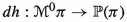of the Hamiltonian section h, as a section of $\mathbb {P}(\pi )$. In addition, an affine bundle epimorphism $A: J^1(\pi \circ \nu ^0) \rightarrow \mathbb {P}(\pi )$ from the 1-jet bundle of the fibration onto $\mathbb {P}(\pi )$ may be also introduced. Then, the solutions of the Hamilton–deDonder–Weyl equations are the sections whose first prolongation $j^1s^0: M \rightarrow J^1(\pi \circ \nu ^0)$ is contained in the submanifold 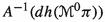(see [42, 43]; see also [45, 60] for the particular case of time-dependent Hamiltonian Mechanics).

1.2 The problem

The previous comments lead naturally to the following question:

Does there exist a completely canonical geometric formulation of the Hamilton–deDonder–Weyl equations which is analogous to the standard Poisson bracket formulation of time-independent Hamiltonian Mechanics?

A possible answer to this question could be the geometric formulation developed in [12] (see Sect. 1.1). However, this formulation is not canonical since most of the constructions in [12] depend on the chosen auxiliary connection in the configuration bundle. In fact, in a previous paper [59] Marsden and Shkoller justify the use of this connection in the geometric formulation of the theory and one may find, in that paper (see [59], page 554), the following cite:

It is interesting that the structure of connection is not necessary to intrinsically define the Lagrangian formalism (as shown in the preceding references), while for the intrinsic definition of a covariant Hamiltonian the introduction of such a structure is essential. Of course, one can avoid a connection if one is willing to confine ones attention to local coordinates.

However, in our paper, we will construct a bracket that does not use any auxiliary objects such as a connection in the configuration bundle and which is completely canonical, thereby giving an affirmative answer to the question above.

1.3 Answer to the problem and contributions of the paper

In order to give an affirmative answer to the question in Sect. 1.2, we will use the following previous contributions and results:

• The construction of the phase space $\mathbb {P}(\pi )$ associated with the configuration bundle $\pi : E \rightarrow M$ and the differential of a Hamiltonian section as a section of $\mathbb {P}(\pi )$ (see [42]).

• The affine bundle epimorphism $A: J^1(\pi \circ \nu ^0) \rightarrow \mathbb {P}(\pi )$ which was also introduced in [42].

• The notion of a Hamiltonian connection associated with a Hamiltonian section h. This type of objects were already considered in [23, 25] in order to characterize the solutions of the Hamilton–deDonder–Weyl equations for h (although the authors of these papers did not use the terminology of a Hamiltonian connection).

We will combine the previous constructions as follows.

As a first step, we consider the affine bundle isomorphism

$$\begin{aligned} \sharp ^\textrm{aff}: \mathbb {P}(\pi ) \rightarrow J^1(\pi \circ \nu ^0)/{\text {Ker}} A \end{aligned}$$

where ${\text {Ker}} A$ is the kernel of the affine bundle epimorphism $A: J^1(\pi \circ \nu ^0) \rightarrow \mathbb {P}(\pi )$ and $\sharp ^\textrm{aff} = \hat{A}^{-1}$, with $\hat{A}: J^1(\pi \circ \nu ^0)/{\text {Ker}} A \rightarrow \mathbb {P}(\pi )$ the affine bundle isomorphism induced by A. Then, we introduce the section

of $J^1(\pi \circ \nu ^0)/{\text {Ker}} A$, given by

$$\begin{aligned} \Gamma _h = \sharp ^\textrm{aff} \circ dh \end{aligned}$$

and we prove the following result: the section $\Gamma _h$ is canonically identified to the equivalence class of Ehresmann connections on the fibration that are Hamiltonian connections for h, see Theorem 3.8.

So, the section $\Gamma _h$ associated to the Hamiltonian section h is the field-theoretic analogue to the Hamiltonian vector field $X_H$ associated to a Hamiltonian function H in Classical Mechanics. The following commutative diagram illustrates the situation

The analogy with the corresponding diagram given in 1.1 for classical mechanics is evident.

The next step is to introduce a suitable space of currents (a vector subspace of $(m-1)$-forms on which are horizontal with respect to the fibration ), in such a way that the restriction of the standard exterior differential to takes values in the space of sections of the vector bundle $(J^1(\pi \circ \nu ^0)/{\text {Ker}} A)^+ = \textrm{Aff}(J^1(\pi \circ \nu ^0)/{\text {Ker}} A, (\pi \circ \nu ^0)^*(\Lambda ^mT^*M))$, that is, we have the linear map

The dual vector bundle $(J^1(\pi \circ \nu ^0)/{\text {Ker}} A)^+$ is chosen so that these differentials can be canonically paired with the Hamiltonian connections $\Gamma _h$, thereby extending to the field-theoretic context the pairing $\left\langle dF, X_H \right\rangle$ between the differential dF of an observable and the Hamiltonian vector field $X_H$, see (1.3). This is our motivation for introducing the space of currents and although it is different to the motivation in [12], just coincides with the space of currents in [12] (see Remark 3.14).

Now, if $\Gamma (\mu )$ is the space of Hamiltonian sections, we can define the linear-affine canonical bracket

(1.6)

given by

Then, one may prove that the evolution of any current along a solution of the Hamilton–deDonder–Weyl equations for h is given by

$$\begin{aligned} (s^0)^*(d\alpha ^0) = \{\alpha ^0, h\} \circ s^0. \end{aligned}$$

(1.7)

Conversely, if is such that (1.7) holds for all , then $s^0$ is a solution of Hamilton–deDonder–Weyl equations. The canonical bracket formulation (1.7) is the field-theoretic analogue to the canonical Poisson bracket formulation (1.2) of classical mechanics.

The previous tasks are performed in Sect. 3.4 (see Theorem 3.15). Here again, the analogy with the canonical Poisson formulation of classical mechanics (see (1.2) and (1.3)) is evident.

It is important to note the affine character of the canonical bracket $\{\cdot , \cdot \}$ in (1.6): the space $\Gamma (\mu )$ of Hamiltonian sections is an affine space modelled over the vector space $\Gamma ((\pi \circ \nu ^0)^*(\Lambda ^mT^*M))$. Recalling that the canonical Poisson bracket on $T^*Q$ induces a Lie algebra structure on $C^{\infty }(T^*Q)$, a new question arises:

What are the algebraic properties of the bracket ?

Related to this question, we will prove that admits a canonical Lie algebra structure (see Theorem 4.2) and that the linear map

defined by

is a representation of the Lie algebra on the affine space $\Gamma (\mu )$ (see Theorem 4.3 and the property (4.13)).

The previous results will be applied to the following examples: time-dependent Hamiltonian systems, Continuum Mechanics (including fluid dynamics and nonlinear elasticity) and Yang–Mills theories. Some of the constructions developed in the paper are illustrated in the Diagram in Appendix §C.

1.4 Structure of the paper

The paper is structured as follows. In Sect. 2, we review the geometric formulation of the Hamilton–deDonder–Weyl equations using the multisymplectic structure on the phase space induced by the Hamiltonian section. In Sect. 3, we introduce the canonical linear-affine bracket and we formulate the Hamilton–deDonder–Weyl equations using this bracket. In particular, we describe the evolution of a current along a solution of the Hamilton–deDonder–Weyl equations. In Sect. 4, we introduce a Lie algebra structure on and we prove that $\{\cdot , \cdot \}$ induces a representation of the Lie algebra on the affine space $\Gamma (\mu )$ of Hamiltonian sections. In Sect. 5, we apply the previous results to several examples. The paper closes with three appendices. In the first one, we review the definition of the 1-jet bundle associated with a fibration, in the second one, we discuss the vertical lift of a section of a vector bundle as a vertical vector field on the total space and, in the third one, we present a Diagram which illustrates most of the relevant constructions in the paper.

2 Hamiltonian classical field theories of first order

In this section, we review some basic constructions and results on Hamiltonian Classical Field Theories of first order (for more details, see [11]).

2.1 The restricted and extended multimomentum bundle associated with a fibration

The configuration bundle of a classical field theory is a fibration $\pi : E \rightarrow M$, that is, a surjective submersion from E to M. We assume $dim \; M = m$ and $dim \; E = m+n$.

The extended multimomentum bundle associated with the configuration bundle $\pi : E \rightarrow M$ is the vector bundle over E whose fiber at the point $y \in E$ is

Here, $J^1\pi = \cup _{y \in E}J^1_y\pi$ is the 1-jet bundle of the fibration $\pi : E \rightarrow M$ (see Appendix A).

It is well-known that may be identified with the vector bundle $\Lambda _2^m(T^*E)$ over E, whose fiber at $y \in E$ is

$$\begin{aligned} \Lambda ^m_2(T_y^*E) = \left\{ \gamma \in \Lambda ^m(T_y^*E) \mid i_ui_{u'} \gamma = 0, \forall u, u' \in V_y\pi \right\} . \end{aligned}$$

In fact, if $\gamma \in \Lambda _2^m (T_y^*E)$ and $z: T_{\pi (y)}M \rightarrow T_yE \in J^1_y \pi$ then

$$\begin{aligned} \langle \gamma , z\rangle = \Lambda ^m z^*(\gamma ). \end{aligned}$$

(2.1)

If $(x^{i}, u^{\alpha })$ are local coordinates on E which are adapted with the fibration $\pi$, then $\gamma \in \Lambda ^m_2(T_y^*E)$ reads locally

$$\begin{aligned} \gamma = p \,d^m x + p^{i}_{\alpha } du^{\alpha } \wedge d^{m-1}x_i, \end{aligned}$$

where

$$\begin{aligned} d^mx = dx^{1} \wedge \cdots \wedge dx^m \; \; \text{ and } \; \; d^{m-1}x_j = i\left( \frac{\partial }{\partial x^j}\right) d^mx. \end{aligned}$$

So, $(x^{i}, u^{\alpha }, p, p_{\alpha }^{i})$ are local coordinates on .

On we can define a canonical m-form as follows

(2.2)

for $\gamma \in \Lambda _2^m(T^*E)$ and $Y_1, \ldots , Y_m \in T_{\gamma }\Lambda ^m_2(T^*E)$, with the vector bundle projection.

From (2.2), has the local expression

The canonical multisymplectic structure on is the $(m+1)$-form given by

Locally, we have

(2.3)

It is clear that is closed and non-degenerate, that is, the vector bundle morphism

is a linear monomorphism.

The restricted multimomentum bundle is the vector bundle

Local coordinates on are $(x^{i}, u^{\alpha }, p_{\alpha }^{i})$.

There is a canonical projection given by

$$\begin{aligned} \mu (\gamma ) = \gamma ^{l}, \end{aligned}$$

for , where $\gamma ^l: T^*_{\pi (y)}M \otimes V_y\pi \rightarrow \Lambda ^{m}T^*_{\pi (y)}M$ is the linear map associated with $\gamma$. The local expression of $\mu$ is

$$\begin{aligned} \mu (x^{i}, u^{\alpha }, p, p_{\alpha }^{i}) = (x^{i}, u^{\alpha }, p_{\alpha }^{i}). \end{aligned}$$

Note that if then

$$\begin{aligned} \mu (\gamma )= & {} \mu (\gamma ') \Leftrightarrow \nu (\gamma ) = \nu (\gamma ') \text{ and } \exists ! \; \Omega \in \Lambda ^mT^*_{\pi (\nu (\gamma ))}M \text{ such } \text{ that } \nonumber \\ \gamma '= & {} \gamma + (\Lambda ^mT^*_{\nu (\gamma )}\pi )(\Omega ). \end{aligned}$$

(2.4)

Remark 2.1

Note that this last statement implies that . This situation recalls a particular case in the Poisson realm, the quotient of a symplectic manifold by a proper and free action of a symmetry Lie group inherits a Poisson structure. In this formalism, the quotient of the extended multimomentum bundle also has a new version of a multi-Poisson structure (see for example [8]) which is defined via a Lie algebroid structure on a subbundle of , when the base manifold M is orientable. Note that, in such a case, if we fix a volume form on M, we have an action of the real line $\mathbb {R}$ on , which preserves the multisymplectic structure, and is the space of orbits of this action. For the definition and details on the construction of the multi-Poisson structure, we refer to [9].

2.2 Hamilton–deDonder–Weyl equations

Given a configuration bundle $\pi : E \rightarrow M$, a Hamiltonian section is a smooth section of the canonical projection

The local expression of h is

$$\begin{aligned} h(x^{i}, u^{\alpha }, p_{\alpha }^{i}) = (x^{i}, u^{\alpha }, -H(x, u, p), p_{\alpha }^{i}), \end{aligned}$$

where H is a local real $C^{\infty }$-function on .

Using the Hamiltonian section, we can define the $(m+1)$-form $\omega _h$ on given by

(2.5)

The local expression of $\omega _h$ is

$$\begin{aligned} \omega _h= & {} du^{\alpha } \wedge dp_{\alpha }^{i} \wedge d^{m-1}x_i + dH \wedge d^mx \nonumber \\= & {} du^{\alpha } \wedge dp_{\alpha }^{i} \wedge d^{m-1}x_i + \frac{\partial H}{\partial u^{\alpha }} du^{\alpha } \wedge d^mx + \frac{\partial H}{\partial p_{\alpha }^{i}} dp_{\alpha }^{i} \wedge d^mx. \end{aligned}$$

(2.6)

Note that if $m = 1$, $\omega _h$ is degenerate and the rank of its kernel is 1. On the other hand, if $m \ge 2$, $\omega _h$ is non-degenerate which implies that it is multisymplectic.

Proposition 2.2

A (local) section of the projection is a solution of the Hamilton–deDonder–Weyl equations iff

$$\begin{aligned} (s^0)^*(i_U\omega _h) = 0, \; \; \; \forall \; U \in \Gamma (V(\pi \circ \nu ^0)), \end{aligned}$$

where $\Gamma (V(\pi \circ \nu ^0))$ is the space of sections of the vertical bundle to .

Proof

Using the local expression $s^0(x^{i}) = (x^{i}, u^{\alpha }(x), p_{\alpha }^{i}(x))$, it is routine to verify that $(s^0)^*(i_U\omega _h) = 0$ if and only if

$$\begin{aligned} \frac{\partial u^{\alpha }}{\partial x^{i}}= & {} \frac{\partial H}{\partial p_{\alpha }^{i}}, \; \; \text{ for } \text{ all } i \text{ and } \alpha ,\\ \sum _{i}\frac{\partial p_{\alpha }^{i}}{\partial x^{i}}= & {} -\frac{\partial H}{\partial u^{\alpha }}, \; \; \text{ for } \text{ all } \alpha . \end{aligned}$$

$\square$

3 A new canonical bracket formulation of Hamiltonian classical field theories of first order

As we reviewed in the Introduction, the phase space of momenta for classical mechanics is the cotangent bundle $T^*Q$ of the configuration space Q, a smooth manifold of dimension n. The cotangent bundle $T^*Q$ carries a canonical symplectic structure which induces a vector bundle isomorphism $\flat : T(T^*Q) \rightarrow T^*(T^*Q)$ over the identity with inverse denoted $\sharp :T^*(T^*Q) \rightarrow T(T^*Q)$. The Hamiltonian is a real $C^{\infty }$-function on $T^*Q$ and the Hamiltonian vector field is given in terms of the differential dH and the vector bundle isomorphism $\sharp$ as $X_H= \sharp dH$, see Diagram (1.1). For field theories, we don’t have a Hamiltonian function, but a Hamiltonian section

of the canonical projection . So, the following questions arise when extending the previous construction to field theories:

Question 1

What is the differential of h?

Question 2

Where does the differential of h take values?

We will answer these questions in Sect. 3.1 by showing that the differential dh of h is a section of the phase bundle $\mathbb {P}(\pi )$ associated with the fibration . The bundle $\mathbb {P}(\pi )$ was introduced in [42] and was used there to discuss a Tulczyjew triple for Classical Field Theories of first order. This will allow us to define the field-theoretic analogue to the vector bundle isomorphism $\sharp$ in Sect. 3.2 and the field-theoretic analogue $\Gamma _h$ to the Hamiltonian vector field $X_H$ in Sect. 3.3. In particular, we will show that $\Gamma _h$ can be identified with the equivalence class of Hamiltonian Ehresmann connections associated to h.

Going back to Classical Hamiltonian Mechanics, we recall that the set of observables is the space $C^\infty (T^*Q)$ and that the Hamilton equations can be equivalently formulated in the Poisson bracket form (1.2) with respect to the canonical Poisson bracket giving by the formulas (1.3). In view of this formulation, we need to find a suitable space of currents for field theories (the observables in field theories) such that their differentials take values in a bundle dual to the target bundle of $\Gamma _h$, this is the goal of Sect. 3.4. From this a canonical bracket can be obtained between currents and Hamiltonian sections. This construction is carried out in Sect. 3.5.

3.1 The phase bundle associated with a fibration and the differential of a Hamiltonian section

Let $\pi : E \rightarrow M$ be the configuration bundle of the field theory and be the Hamiltonian section. Then, although

h cannot be identified, in general, with a real $C^{\infty }$-function on . However, to h we can associate an extended Hamiltonian density

defined as follows. If we have $\mu (\gamma ) = \mu (h(\mu (\gamma )))$ and hence using (2.4), we conclude that there exists a unique $\Omega \in \Lambda ^mT^*_{\pi (\nu (\gamma ))}M$ such that $\gamma = h(\mu (\gamma )) + (\Lambda ^mT^*_{\nu (\gamma )}\pi )(\Omega )$. We thus define

3.1.1 The differential of and the extended phase bundle

Note that may be considered, in a natural way, as a m-form on . Thus, we can take its exterior differential and we obtain a $(m+1)$-form on which is a section of the vector bundle

Now, it is easy to prove that the vector bundles and $V^*(\pi \circ \nu ) \otimes (\pi \circ \nu )^*(\Lambda ^mT^*M)$ are isomorphic. In fact, an isomorphism

is given by

$$\begin{aligned} \Psi (\tilde{\theta }): V_{\gamma }(\pi \circ \nu ) \rightarrow \Lambda ^m(T^*_{\pi (\nu (\gamma ))}M), \; \; \tilde{U} \in V_{\gamma }(\pi \circ \nu ) \rightarrow i_{\tilde{U}}\tilde{\theta } \in \Lambda ^m(T^*_{\pi (\nu (\gamma ))}M), \end{aligned}$$

for and . Note that , therefore, it induces an element of $\Lambda ^m(T^*_{\pi (\nu (\gamma ))}M)$.

We denote by the section of the vector bundle induced by the differential of . In local coordinates, if

$$\begin{aligned} h(x^{i}, u^{\alpha }, p_{\alpha }^{i}) = (x^{i}, u^{\alpha }, -H(x, u, p), p_\alpha ^{i}) \end{aligned}$$

then

(3.1)

and

(3.2)

Note that if is the canonical projection, $\Phi$ is a m-form on M and $\Phi ^\textbf{v} \in \Gamma (V\mu )$ is the vertical lift to (see Appendix B) then, using (3.2) and (B.1), we deduce that

(3.3)

This property of motivates the definition of the following affine subbundle of $V^*(\pi \circ \nu ) \otimes (\pi \circ \nu )^*(\Lambda ^mT^*M)$.

Definition 3.1

The extended phase bundle of the configuration bundle $\pi : E \rightarrow M$ is the affine subbundle $\widetilde{\mathbb {P}(\pi )}$ of $V^*(\pi \circ \nu ) \otimes (\pi \circ \nu )^*(\Lambda ^mT^*M)$ whose fiber at the point is

(3.4)

From (3.3) we have

Note that $\widetilde{\mathbb {P}(\pi )}$ is modelled over the vector bundle $V(\widetilde{\mathbb {P}(\pi )})$ whose fiber at the point is

$$\begin{aligned} V(\widetilde{\mathbb {P}(\pi )})(\gamma ) = \{ \tilde{\nu }\in {\text {Lin}}(V_{\gamma }(\pi \circ \nu ), \Lambda ^mT^*_{\pi (\nu (\gamma ))}M) \mid \tilde{\nu }(\Omega ^\textbf{v}(\gamma )) = 0, \forall \;\Omega \in \Lambda ^mT^*_{\pi (\nu (\gamma ))}M \}. \end{aligned}$$

We remark that an element of $\widetilde{\mathbb {P}(\pi )}$ has the following local form

and a generic element $\tilde{\nu }$ of $V(\widetilde{\mathbb {P}(\pi )})$ has the local form

Therefore, the local coordinates on $\widetilde{\mathbb {P}(\pi )}$ and $V(\widetilde{\mathbb {P}(\pi )})$ are . In addition,

(3.5)

3.1.2 The differential of a Hamiltonian section and the phase bundle

Now, given a point $x \in M$, we can consider an action of the abelian group $\Lambda ^mT^*_xM$ on the fiber $(\pi \circ \nu )^{-1}(x)$ defined as follows. If $\Phi \in \Lambda ^m(T^*_{x}M)$ then we define $\Phi \; \cdot : (\pi \circ \nu )^{-1}(x) \rightarrow (\pi \circ \nu )^{-1}(x)$ by

$$\begin{aligned} \Phi \cdot \gamma = \gamma + (\Lambda ^mT^*_{\nu (\gamma )}\pi )(\Phi ), \; \; \text{ for } \gamma \in (\pi \circ \nu )^{-1}(x). \end{aligned}$$

(3.6)

In local coordinates, we get

$$\begin{aligned} (\lambda d^mx)\cdot (x^{i}, u^{\alpha }, p, p_{\alpha }^{i}) = (x^{i}, u^{\alpha }, p + \lambda , p_{\alpha }^{i}) \end{aligned}$$

and thus the quotient space may be identified with the reduced multimomentum bundle .

The tangent and cotangent lift of the previous action induces a fibred action of the vector bundle $(\pi \circ \nu )^*(\Lambda ^mT^*M)$ on the vector bundles $V(\pi \circ \nu )$ and $V^*(\pi \circ \nu ) \otimes (\pi \circ \nu )^*(\Lambda ^mT^*M)$. In fact, if $\gamma \in \Lambda ^m_2(T^*_yE)$, $\tilde{U} \in V_\gamma (\pi \circ \nu )$ and $\Phi \in \Lambda ^mT^*_{\pi (y)}M$ then the tangent lift is

$$\begin{aligned} \Phi \; \cdot \tilde{U} = (T_{\gamma }(\Phi \cdot ))(\tilde{U}) \in V_{\Phi \cdot \gamma }(\pi \circ \nu ). \end{aligned}$$

(3.7)

Note that, using (3.6), (3.7) and (B.1), it follows that

$$\begin{aligned} \Phi \cdot \Omega ^\textbf{v}_{\gamma } = \Omega ^\textbf{v}_{\Phi \cdot \gamma }, \end{aligned}$$

(3.8)

for $\Omega \in \Lambda ^mT^*_{\pi (y)}M$. If $(x^{i}, u^{\alpha }, p, p_{\alpha }^{i}; \dot{u}^{\alpha }, \dot{p}, \dot{p}_{\alpha }^{i})$ are local coordinates on $V(\pi \circ \nu )$, we have

$$\begin{aligned} (\lambda d^m x)\cdot (x^{i}, u^{\alpha }, p, p_{\alpha }^{i}; \dot{u}^{\alpha }, \dot{p}, \dot{p}_{\alpha }^{i}) = (x^{i}, u^{\alpha }, p + \lambda , p_{\alpha }^{i}; \dot{u}^{\alpha }, \dot{p}, \dot{p}_{\alpha }^{i}). \end{aligned}$$

(3.9)

In a similar way, if $\tilde{\theta } \in V^{*}_{\gamma }(\pi \circ \nu ) \otimes \Lambda ^mT^*_{\pi (\nu (\gamma ))}M$ then the cotangent lift is

$$\begin{aligned} (\Phi \cdot \tilde{\theta }) (\tilde{U}') = \tilde{\theta }(-\Phi \cdot \tilde{U}'), \end{aligned}$$

(3.10)

for $\tilde{U}' \in V_{\Phi \cdot \gamma }(\pi \circ \nu )$. From (3.4) and (3.8), we deduce that this action restricts to the extended phase bundle $\widetilde{\mathbb {P}(\pi )}$, and to the vector bundle $V(\widetilde{\mathbb {P}(\pi )})$. In local coordinates, we have

Taking the quotient with respect to the action, we can introduce the following definition.

Definition 3.2

The phase bundle of the configuration bundle $\pi : E \rightarrow M$ is defined by

$$\begin{aligned} \displaystyle \mathbb {P}(\pi ) = \frac{\widetilde{\mathbb {P}(\pi )}}{(\pi \circ \nu )^*(\Lambda ^mT^*M)}. \end{aligned}$$

We note that $\mathbb {P}(\pi )$ is an affine bundle over modelled over the vector bundle $\displaystyle V(\mathbb {P}(\pi )) = \frac{V(\widetilde{\mathbb {P}(\pi ))}}{(\pi \circ \nu )^*(\Lambda ^mT^*M)}$. This bundle is isomorphic to the vector bundle

an isomorphism being given by

where is defined by

with and $\mu (\gamma ) = \gamma ^0$. Local coordinates on $\mathbb {P}(\pi )$ and $V({\mathbb {P}(\pi ))}$ are

(3.11)

It is clear that there exists a one-to-one correspondence between the space of sections of the affine bundle and the set of sections of the extended phase bundle $\widetilde{\mathbb {P}(\pi )}$ associated with $\pi$, which are $(\pi \circ \nu )^*(\Lambda ^mT^*M)$-equivariant. So, if is a Hamiltonian section then, using (3.5), it is easy to see that the vertical differential is $(\pi \circ \nu )^*(\Lambda ^mT^*M)$-equivariant and, therefore, it induces a section

of the phase bundle $\mathbb {P}(\pi )$. We can thus write the following definition.

Definition 3.3

The differential of a Hamiltonian section is the section

defined by the following commutative diagram

where and $\tilde{\mu }: \widetilde{\mathbb {P}(\pi )} \rightarrow \mathbb {P}(\pi )$ are the canonical projections.

The local expression of dh is

$$\begin{aligned} dh(x^{i}, u^{\alpha }, p_{\alpha }^{i}) = \Big (x^{i}, u^{\alpha }, p_{\alpha }^{i}; \frac{\partial H}{\partial u^{\alpha }}, \frac{\partial H}{\partial p_{\alpha }^{i}}\Big ). \end{aligned}$$

(3.12)

So, we have given an answer to Questions 1 and 2 stated above.

From the previous definition, we get the map

$$\begin{aligned} d: \Gamma (\mu ) \rightarrow \Gamma (\mathbb {P}(\pi )),\quad h \in \Gamma (\mu ) \rightarrow dh \in \Gamma (\mathbb {P}(\pi )). \end{aligned}$$

Note that $\Gamma (\mu )$ and $\Gamma (\mathbb {P}(\pi ))$ are affine spaces modelled over the vector spaces $\Gamma ((\pi \circ \nu ^0)^*(\Lambda ^mT^*M))$ and $\Gamma (V(\mathbb {P}(\pi )))$, respectively, and d is an affine map. Later in the paper, we shall use the corresponding linear map $d^l: \Gamma ((\pi \circ \nu ^0)^*(\Lambda ^mT^*M))\rightarrow \Gamma (V(\mathbb {P}(\pi )))$ defined as follows. If is a $(\pi \circ \nu ^0)^*(\Lambda ^mT^*M)$-valued function on then it may be considered as a section of the vector bundle

So, we can take the standard differential and we obtain a section of the vector bundle

This vector bundle is isomorphic to , an isomorphism

is given by

$$\begin{aligned} \Psi ^0(\theta ): V_{{\gamma }^0}(\pi \circ \nu ^0) \rightarrow \Lambda ^m(T^*_{\pi (\nu ^0(\gamma ^0))}M), \; \; U \rightarrow i_{U}\theta , \end{aligned}$$

for and . Note that and, therefore, it induces an element of $\Lambda ^m(T^*_{\pi (\nu ^0(\gamma ^0))}M)$. We denote by the section of the vector bundle induced by the differential via the isomorphism $\Psi ^0$. If locally

the local expression of is

(3.13)

3.1.3 Comments on the next steps

The differential of a Hamiltonian section is the field theoretic analogue to the differential $dH: T^*Q \rightarrow T^*(T^*Q)$ of a Hamiltonian function in classical mechanics. In the next section, we will introduce a quotient affine bundle which is the field theoretic analogue to the tangent bundle $T(T^*Q)$ of the phase space in classical mechanics. Recall that using the canonical symplectic structure of $T^*Q$, one can define a canonical vector bundle isomorphism

$$\begin{aligned} \sharp : T^*(T^*Q) \rightarrow T(T^*Q) \end{aligned}$$

and the Hamiltonian vector field $X_H$ on $T^*Q$ associated with a Hamiltonian function $H \in C^{\infty }(T^*Q)$ is given by $X_H = \sharp \circ dH$. So, a natural question arises:

Question 3

Does there exist an affine bundle isomorphism $\sharp ^\textrm{aff}: \mathbb {P}(\pi ) \rightarrow J^{1}(\pi \circ \nu ^0)/ {\text {Ker}} A$ which, in the presence of a Hamiltonian section , allows us to introduce a distinguished section $\Gamma _h$ of the affine bundle ?

In the next Sect. 3.2, we will give an affirmative answer to Question 3 and we will discuss the relation between $\Gamma _h$ and the solutions of the Hamilton–deDonder–Weyl equations for h. The section $\Gamma _h$ will play the role of $X_H$ in Hamiltonian Mechanics.

3.2 The field-theoretic analogue to the canonical isomorphism $\sharp : T^*(T^*Q) \rightarrow T(T^*Q)$

We will show that it is given by an affine bundle isomorphism $\sharp ^\textrm{aff}: \mathbb {P}(\pi ) \rightarrow J^{1}(\pi \circ \nu ^0)/ {\text {Ker}} A$.

Let $J^1(\pi \circ \nu ^0)$ be the 1-jet bundle associated with the fibration (see Appendix A). To define the quotient affine bundle, we shall use a construction in [42]. In this paper, the author introduced an affine bundle epimorphism

$$\begin{aligned} A: J^{1}(\pi \circ \nu ^0) \rightarrow \displaystyle \mathbb {P}(\pi ) = \frac{\widetilde{\mathbb {P}(\pi )}}{(\pi \circ \nu )^*(\Lambda ^mT^*M)} \end{aligned}$$

over the identity of . This epimorphism is constructed in several steps.

First, we consider the vector bundle monomorphism

induced by the canonical multisymplectic structure as follows

(3.14)

Note that, from (2.3), there exists a unique m-form at $\mu (\gamma )$ on , which we denote by $\bar{\flat }(\tilde{U})$, such that

(3.15)

This defines a vector bundle morphism

over the canonical projection . Using local coordinates $(x^{i}, u^\alpha , p, p_\alpha ^{i}; \dot{u^\alpha }, \dot{p}, \dot{p}_\alpha ^{i})$ and $(x^{i}, u^\alpha , p_\alpha ^{i}; \bar{p}, \bar{p}_\alpha ^{i}, \bar{p}_i^{\alpha j})$ on $V(\pi \circ \nu )$ and , respectively, the local expression of $\bar{\flat }$ is

$$\begin{aligned} \bar{\flat }(x^{i}, u^\alpha , p, p_\alpha ^{i}; \dot{u^\alpha }, \dot{p}, \dot{p}_\alpha ^{i}) = (x^{i}, u^\alpha , p_\alpha ^{i}; -\dot{p}, -\dot{p}_\alpha ^{i}, \bar{p}_i^{\alpha j} = \dot{u}^\alpha \delta ^j_i). \end{aligned}$$

(3.16)

If , the following commutative diagram

(3.17)

illustrates the relation between $\tilde{\flat }$ and $\bar{\flat }$.

We shall now use the vector bundle morphism $\bar{\flat }$ to construct A. For and $Z^0\in J^1_{\gamma ^0}(\pi \circ \nu ^0)$ one first defines

$$\begin{aligned} \widetilde{A(Z^0)} \in \widetilde{\mathbb {P}(\pi )}(\gamma ) \subseteq V_{\gamma }^*(\pi \circ \nu ) \otimes \Lambda ^mT^*_{\pi (\nu (\gamma ))}M, \end{aligned}$$

with such that $\mu (\gamma ) = \gamma ^0$, as follows:

$$\begin{aligned} \big \langle \widetilde{A(Z^0)}, \tilde{U} \big \rangle = - \Lambda ^m((Z^0)^*)(\bar{\flat }(\tilde{U})), \end{aligned}$$

(3.18)

for $\tilde{U} \in V_\gamma (\pi \circ \nu )$. Then, if $\tilde{\mu }: \widetilde{\mathbb {P}(\pi )} \rightarrow \mathbb {P}(\pi )$ is the canonical projection, we set

$$\begin{aligned} A(Z^0) = \tilde{\mu }(\widetilde{A(Z^0)}). \end{aligned}$$

(3.19)

Note that A is well-defined and its local expression is

$$\begin{aligned} A(x^{i}, u^{\alpha }, p_{\alpha }^{i}; u^{\alpha }_j, p_{\alpha j}^{i}) = \Big (x^{i}, u^{\alpha }, p_{\alpha }^{i}; - \sum _{i} p^{i}_{\alpha i}, u^{\alpha }_j\Big ). \end{aligned}$$

(3.20)

This proves that A is an affine bundle epimorphism over the identity of (for more details, see [42]).

Recall that the affine bundle is modelled over the vector bundle . We denote by $(x^{i}, u^{\alpha }, p_\alpha ^{i}; u^\alpha _j, p^{i}_{\alpha j})$ the standard coordinates on $J^1(\pi \circ \nu ^0)$ and $V(J^1(\pi \circ \nu ^0))$ (see Appendix A). From the local expression (3.20), it follows that the kernel of A is a vector subbundle of $V(J^1(\pi \circ \nu ^0))$ which is locally characterized by

$$\begin{aligned} {\text {Ker}} A = \left\{ (x^{i}, u^{\alpha }, p_\alpha ^{i}; u^\alpha _j, p^{i}_{\alpha j}) \in V(J^1(\pi \circ \nu ^0)) \mid u^\alpha _j = 0, \sum _i p_{\alpha i}^{i} = 0, \forall \alpha , i\right\} .\nonumber \\ \end{aligned}$$

(3.21)

We can thus consider the quotient affine bundle which is modelled over the quotient vector bundle . From (3.21), we have that a local basis of sections for this vector bundle is

$$\begin{aligned} \left\{ \nu _{\alpha }^i = \left[ dx^{i} \otimes \frac{\partial }{\partial u^{\alpha }}\right] , \nu ^\alpha = 1/m\left[ dx^{1} \otimes \frac{\partial }{\partial p_{\alpha }^1} + \cdots + dx^m \otimes \frac{\partial }{\partial p_{\alpha }^m}\right] \right\} \end{aligned}$$

for $i \in \{1, \ldots , m\}$ and $\alpha \in \{1, \ldots , n\}$. Note that in the quotient vector bundle

$$\begin{aligned} \left[ dx^{i} \otimes \frac{\partial }{\partial p_{\alpha }^i}\right] = \left[ dx^{j} \otimes \frac{\partial }{\partial p_{\alpha }^j}\right] , \; \; \forall \; i, j \text{ and } \alpha . \end{aligned}$$

Local coordinates associated to this basis of sections on the quotient vector bundle (and also on the quotient affine bundle $J^1(\pi \circ \nu ^0)/ {\text {Ker}} A$) are denoted $(x^{i}, u^{\alpha }, p_{\alpha }^{i}; \hat{u}^{\alpha }_j, \hat{p}_{\alpha })$

The affine bundle epimorphism $A: J^1(\pi \circ \nu ^0) \rightarrow \mathbb {P}(\pi )$ induces an affine bundle isomorphism

$$\begin{aligned} \hat{A}: J^1(\pi \circ \nu ^0)/{\text {Ker}} A \rightarrow \mathbb {P}(\pi ) \end{aligned}$$

and, from (3.20), we deduce that the local expression of $\hat{A}$ is

$$\begin{aligned} \hat{A}(x^{i}, u^\alpha , p_\alpha ^{i}; \hat{u}^\alpha _i, \hat{p}_\alpha ) = (x^{i}, u^\alpha , p_\alpha ^{i}; -\hat{p}_\alpha , \hat{u}^\alpha _i). \end{aligned}$$

(3.22)

By definition, the affine bundle isomorphism

$$\begin{aligned} \sharp ^\textrm{aff}: \mathbb {P}(\pi ) \rightarrow J^1(\pi \circ \nu ^0) /{\text {Ker}} A \end{aligned}$$

is the inverse isomorphism to $\hat{A}: J^1(\pi \circ \nu ^0) /{\text {Ker}} A \rightarrow \mathbb {P}(\pi )$. If we consider the local coordinates on the phase bundle $\mathbb {P}(\pi )$ then, using (3.22), it follows that

(3.23)

3.3 The field-theoretic analogue to the Hamiltonian vector field $X_H:TQ \rightarrow T(T^*Q)$

Let be a Hamiltonian section. We have seen that the differential of h

is a section of the phase bundle $\mathbb {P}(\pi )$. So, we can define the section

of the quotient affine bundle by

$$\begin{aligned} \Gamma _h = \sharp ^\textrm{aff} \circ dh. \end{aligned}$$

(3.24)

Using (3.12), (3.23) and the local basis of sections $\{\nu _\alpha ^i, \nu ^\alpha \}$ introduced above, we obtain that the local expression of $\Gamma _h$ is

$$\begin{aligned} \Gamma _h - \left[ dx^{i} \otimes \frac{\partial }{\partial x^{i}}\right] = \frac{\partial H}{\partial p_{\alpha }^i} \nu ^{i}_{\alpha } - \frac{\partial H}{\partial u^{\alpha }} \nu ^{\alpha }. \end{aligned}$$

(3.25)

Now, we will show that $\Gamma _h$ plays the same role, in Hamiltonian Classical Field Theories of first order, that the Hamiltonian vector field associated with a Hamiltonian function in Classical Mechanics. This will give an affirmative answer to Question 3 in Sect. 3.1.

For this purpose, we will discuss the relation between $\Gamma _h$ and the solutions of the Hamilton–deDonder–Weyl equations for h. This uses the notion of a Hamiltonian connection (see [23, 25]).

Let $\tau : N \rightarrow B$ be an arbitrary fibration and H an Ehresmann connection on $\tau : N \rightarrow B$. Denote by $^H: N \times _B TB \rightarrow H \subseteq TN$ the horizontal lift induced by H (see Appendix A). It is clear that if $1 \le r \le b = {\text {dim}} B$ the previous map induces a vector bundle isomorphism between $N \times _B \Lambda ^r(TB)$ and $\Lambda ^r H$ which we also denote by

$$\begin{aligned} {}^H: N \times _B \Lambda ^r(TB) \rightarrow \Lambda ^rH \subseteq \Lambda ^r(TN). \end{aligned}$$

So, if $\chi \in \Gamma (N \times _B \Lambda ^r(TB))$, the image $\chi ^H$ of $\chi$ by the previous map is called the horizontal lift of $\chi$. If $(b^{i}, n^{\alpha })$ are local coordinates on N which are adapted to the fibration $\tau$, then the horizontal lift reads locally

$$\begin{aligned} \left( \frac{\partial }{\partial b^{i}}\right) ^H = \frac{\partial }{\partial b^{i}} + H^{\alpha }_i\frac{\partial }{\partial n^{\alpha }}, \; \; \forall i \in \{1, \ldots , b\} \end{aligned}$$

and if

$$\begin{aligned} \chi = \chi _{i_1 \ldots i_r}\frac{\partial }{\partial b^{i_1}} \wedge \cdots \wedge \frac{\partial }{\partial b^{i_r}} \in \Gamma (\Lambda ^rTB) \end{aligned}$$

then its horizontal lift is

$$\begin{aligned} \chi ^H= & {} \chi _{i_1 \ldots i_r} \left( \frac{\partial }{\partial b^{i_1}}\right) ^H \wedge \cdots \wedge \left( \frac{\partial }{\partial b^{i_r}}\right) ^H \\= & {} \chi _{i_1 \ldots i_r}\left( \frac{\partial }{\partial b^{i_1}} + H_{i_1}^{\alpha _1} \frac{\partial }{\partial n^{\alpha _1}}\right) \wedge \cdots \wedge \left( \frac{\partial }{\partial b^{i_r}} + H_{i_r}^{\alpha _r} \frac{\partial }{\partial n^{\alpha _r}}\right) . \end{aligned}$$

Now, suppose that $\pi : E \rightarrow M$ is the configuration bundle of a Hamiltonian Classical Field Theory of first order, with $m = {\text {dim}} M$, and consider the fibration . For a Hamiltonian section , we denote by $\omega _h$ the $(m+1)$-form on given by (2.5).

Then, we may prove the following result.

Lemma 3.4

Let be a Hamiltonian section, let H be an Ehresmann connection on the fibration , and let be a section horizontal with respect to H. Then, $s^0$ is a solution of the Hamilton–deDonder–Weyl equations for h if and only if

$$\begin{aligned} (s^0)^*\left( i_{\chi ^H}\omega _h\right) = 0, \; \; \forall \;\chi \in \Gamma (\Lambda ^m(TM)). \end{aligned}$$

(3.26)

Proof

Using that $s^0$ is horizontal with respect to H we deduce that

$$\begin{aligned} (s^0)^*(i_U \omega _h) = 0, \; \; \forall \;U \in \Gamma (V(\pi \circ \nu ^0)) \end{aligned}$$

if and only if

$$\begin{aligned} (s^0)^*\left( i_{\chi ^H}i_U \omega _h \right) = 0, \; \; \forall \;\chi \in \Gamma (\Lambda ^m(TM)). \end{aligned}$$

(3.27)

So, it is clear that if (3.26) holds then $s^0$ is a solution of the Hamilton–deDonder–Weyl equations for h by Proposition 2.2.

Conversely, assume that $s^0$ is a solution of the Hamilton–deDonder–Weyl equations for h. Then (3.27) holds. Thus, using that

we deduce that

$$\begin{aligned} (s^0)^*\left( i_{\chi ^H}\omega _h\right) (x) = 0, \; \; \forall \chi \in \Gamma (\Lambda ^mTM), \; \; \forall x \in U \subseteq M. \end{aligned}$$

This proves the result. $\square$

The previous result suggests the introduction of the following definition.

Definition 3.5

Let be a Hamiltonian section. An Ehresmann connection on the fibration is said to be a Hamiltonian connection for h if

$$\begin{aligned} i_{\chi ^H}\omega _h = 0, \; \; \forall \chi \in \Gamma (\Lambda ^mTM). \end{aligned}$$

As a direct consequence of the definition, if locally the Hamiltonian section h is

$$\begin{aligned} h(x^{i}, u^{\alpha }, p_{\alpha }^{i}) = (x^{i}, u^{\alpha }, -H(x, u, p), p_{\alpha }^{i}) \end{aligned}$$

and the Ehresmann connection is

$$\begin{aligned} \left( \frac{\partial }{\partial x^{i}}\right) ^H = \frac{\partial }{\partial x^{i}} + H_{i}^{\alpha } \frac{\partial }{\partial u^{\alpha }} + H_{\alpha i}^j \frac{\partial }{\partial p_{\alpha }^{j}}, \end{aligned}$$

then from (2.6), we have the equivalence

(3.28)

So, our definition of a Hamiltonian connection is equivalent to that introduced in [23, 25]. Note that a Hamiltonian connection H for h may be identified with a section of the affine bundle (see Appendix A). Moreover, if $\Gamma _h$ is the section of the quotient affine bundle defined in (3.24) then, using (3.25) and (3.28), we obtain the following result.

Proposition 3.6

Let be the section of the affine bundle induced by a Hamiltonian connection H for h and $p: J^1(\pi \circ \nu ^0) \rightarrow J^1(\pi \circ \nu ^0) / {\text {Ker}} A$ be the canonical projection. Then

$$\begin{aligned} \Gamma _h = p \circ s^H. \end{aligned}$$

From (3.21) and (3.28), we also get the following result.

Proposition 3.7

If are Hamiltonian connections for the same Hamiltonian section , then they satisfy

$$\begin{aligned} \bar{H} - H \in \Gamma ({\text {Ker}} A). \end{aligned}$$

Finally, from Propositions 3.6 and 3.7, it follows the following characterization of Hamiltonian connections for h.

Theorem 3.8

Let be a Hamiltonian section and let H be an Ehresmann connection for the fibration . Then, H is a Hamiltonian connection for h if and only if

$$\begin{aligned} \Gamma _h = p \circ s^H. \end{aligned}$$

Theorem 3.8 suggests the introduction of the following definition.

Definition 3.9

Let be a Hamiltonian section. Then, the section is called the equivalence class of the Hamiltonian connections for  h.

The following commutative diagram illustrates the results obtained in Sects. 3.1, 3.2, 3.3

It is the field-theoretic analogue to Diagram 1.1 for Hamiltonian Mechanics.

The last step is to introduce a suitable space of currents for Hamiltonian Classical Field Theories of first order and a suitable canonical bracket formulation for the evolution of such currents along the solution of the Hamilton–deDonder–Weyl equations. This is the aim of the next two subsections.

3.4 A suitable space of currents for Hamiltonian classical field theories

We shall define a space of currents for Hamiltonian Classical Field Theories of first order, which plays the same role that the space of observables in Hamiltonian Mechanics.

Recall that in Hamiltonian Mechanics, the Hamiltonian vector field $X_H$ is a section of the vector bundle $T(T^*Q) \rightarrow T^*Q$ and the space of observables is the set $C^{\infty }(T^*Q)$ of real $C^{\infty }$-functions on $T^*Q$. Given an observable $F \in C^{\infty }(T^*Q)$, we can consider a section dF (the differential of F) of the dual bundle $T^*(T^*Q) \rightarrow T^*Q$ to $T(T^*Q) \rightarrow T^*Q$ and the evolution of the observable F along a solution $s: I \subseteq \mathbb {R} \rightarrow T^*Q$ of Hamilton’s equation is given as

$$\begin{aligned} \frac{d}{dt} (F\circ s)= \langle dF, X_H \rangle \circ s. \end{aligned}$$

When written for all observables F, the previous equations are equivalent to the Hamilton equations.

Our goal is to carry out these construction for Hamiltonian Classical Field theories. As we have seen, given a Hamiltonian section , the object corresponding to the Hamiltonian vector field $X_H$ is the section $\Gamma _h$ of the quotient affine bundle . So, we need to overcome the following two steps:

First step: Describe the dual vector bundle $(J^{1}(\pi \circ \nu ^0)/ {\text {Ker}} A)^+$ to the affine bundle .

Second step: Introduce a space of currents and a differential operator

(3.29)

on this space, such that the evolution of a current along a solution is given by

$$\begin{aligned} (s^0)^*(d\alpha ^0) = \langle d\alpha ^0, \Gamma _h \rangle \circ s^0. \end{aligned}$$

We will show that $s^0$ satisfies these equations for any if and only if $s^0$ is a solution of the Hamilton–deDonder–Weyl equations.

First step: Let $A: J^{1}(\pi \circ \nu ^0) \rightarrow \mathbb {P}(\pi )$ (respectively, $\hat{A}: J^1(\pi \circ \nu ^0)/{\text {Ker}} A \rightarrow \mathbb {P}(\pi )$) be the affine bundle epimorphism (respectively, isomorphism) considered in Sect. 3.2. Denote by $\mathbb {P}(\pi )^+$ and $J^1(\pi \circ \nu ^0)^+$ the vector bundles over defined by

$$\begin{aligned} \mathbb {P}(\pi )^+&= \textrm{Aff}(\mathbb {P}(\pi ), (\pi \circ \nu ^0)^*(\Lambda ^mT^*M))\\ J^1(\pi \circ \nu ^0)^+&= \textrm{Aff}(J^1(\pi \circ \nu ^0), (\pi \circ \nu ^0)^*(\Lambda ^mT^*M)). \end{aligned}$$

It is clear that A induces the vector bundle morphism

for $U^0 \in \mathbb {P}(\pi )^+_{\gamma ^0}$ and $Z^0 \in J^1_{\gamma ^0}(\pi \circ \nu ^0)$, with . Since A is an epimorphism, we deduce that $A^+$ is a vector bundle monomorphism. In addition, the image of $A^+$ is the vector subbundle of $J^1(\pi \circ \nu ^0)^+$ whose fiber at the point is

$$\begin{aligned} A^+(\mathbb {P}(\pi )^+)_{\gamma ^0}= & {} \big \{\theta ^0 \in \textrm{Aff}(J^1_{\gamma ^0}(\pi \circ \nu ^0), \Lambda ^mT^*_{\pi (\nu ^0(\gamma ^0))}M) \mid \\{} & {} \quad \big \langle (\theta ^0)^{l}, {\text {Ker}} A \cap V_{\gamma ^0}(J^1(\pi \circ \nu ^0))\big \rangle = 0\big \}. \end{aligned}$$

Here, $(\theta ^0)^l: V_{\gamma ^0}(J^1(\pi \circ \nu ^0)) \rightarrow \Lambda ^mT^*_{\pi (\nu ^0(\gamma ^0))}M$ denotes the linear map associated with the affine map $\theta ^0: J^1_{\gamma ^0}(\pi \circ \nu ^0) \rightarrow \Lambda ^mT^*_{\pi (\nu ^0(\gamma ^0))}M$. So, we have a vector bundle isomorphism

over the identity of .

Now, denote by $\hat{A}^+: \mathbb {P}(\pi )^+ \rightarrow (J^{1}(\pi \circ \nu ^0)/ {\text {Ker}} A)^+$ the vector bundle isomorphism induced by $\hat{A}: J^{1}(\pi \circ \nu ^0)/ {\text {Ker}} A \rightarrow \mathbb {P}(\pi )$. Then, it is clear that the vector bundles $A^+(\mathbb {P}(\pi )^+)$ and $(J^{1}(\pi \circ \nu ^0)/ {\text {Ker}} A)^+$ can be identified and, under this identification, $\hat{A}^+$ is just the vector bundle isomorphism .

The following commutative diagram

illustrates the situation.

It is desirable to have an explicit realisation of dual vector bundle $(J^{1}(\pi \circ \nu ^0)/ {\text {Ker}} A)^+$. As we know

(see Sect. 2.1). So it is possible to describe $A^+(\mathbb {P}(\pi )^+)$ and, therefore, $(J^{1}(\pi \circ \nu ^0)/ {\text {Ker}} A)^+$, as a certain vector subbundle L of . We shall now give such a description.

First of all, using (3.4), it follows that the vector bundle

$$\begin{aligned} \widetilde{\mathbb {P}(\pi )}^+ = \textrm{Aff} \big (\widetilde{\mathbb {P}(\pi )}, (\pi \circ \nu )^*(\Lambda ^mT^*M)\big ) \end{aligned}$$

is isomorphic to the vertical bundle $V(\pi \circ \nu )$ of the fibration . An isomorphism

is given by

(3.30)

with .

Now, if we consider the standard fibred actions of $(\pi \circ \nu )^*(\Lambda ^mT^*M)$ on $V(\pi \circ \nu )$ and $\widetilde{\mathbb {P}(\pi )}^+$ then, it is clear that is $(\pi \circ \nu )^*(\Lambda ^mT^*M)$-equivariant and, thus, it induces a vector bundle isomorphism

over the identity of . Then, from Definition 3.2, we deduce that the quotient vector bundle $\widetilde{\mathbb {P}(\pi )}^+/(\pi \circ \nu )^*(\Lambda ^mT^*M)$ is isomorphic to $\mathbb {P}(\pi )^+$. So, we have a vector bundle isomorphism

which is characterized by the following condition

(3.31)

for $\tilde{U} \in V_{\gamma }(\pi \circ \nu )$ and , with and $\tilde{\mu }: \widetilde{\mathbb {P}(\pi )} \rightarrow \mathbb {P}(\pi )$ the canonical projection.

We now consider the composition

of the two vector bundles isomorphisms $A^+$ and defined above and show that can be expressed in a simple way, which allows to describe its image L explicitly.

Consider the vector bundle morphism defined in Sect. 3.2 which is characterized by Eq. (3.15) and has the local expression (3.16). Using (3.9), we deduce that $\bar{\flat }$ induces the vector bundle morphism

over the identity of given by

$$\begin{aligned} \flat [\tilde{U}] = \bar{\flat }(\tilde{U}), \; \; \text{ for } \tilde{U} \in V(\pi \circ \nu ). \end{aligned}$$

(3.32)

So, if and is the canonical isomorphism between the fibers by $\gamma$ and $\mu (\gamma )$ of the vector bundles and , then the following diagram

(3.33)

is commutative

Proposition 3.10

We have the equality

(3.34)

This implies that the vector bundle $(J^1(\pi \circ \nu ^0)/ {\text {Ker}} A)^+$ is isomorphic to the vector subbundle L of given by

$$\begin{aligned} L = \bar{\flat }(V(\pi \circ \nu )). \end{aligned}$$

(3.35)

In particular, a local basis of sections of the vector subbundle L is

$$\begin{aligned} \left\{ d^mx, du^\alpha \wedge d^{m-1}x_i, \sum _i dp_\alpha ^{i} \wedge d^{m-1}x_i\right\} . \end{aligned}$$

(3.36)

Proof

If , $\tilde{U} \in V_\gamma (\pi \circ \nu )$ and $Z^0 \in J^1_{\mu (\gamma )}(\pi \circ \nu ^0)$ then, from (3.19), we obtain

Therefore, using (3.30) and (3.31), it follows that

So, from (2.1), (3.18) and (3.32), we conclude that

This proves (3.34).

From this, (3.35) follows using (3.32) and (3.34).

Finally, the local expression is obtained by using (3.16) and (3.35). $\square$

Second step: The previous result together with (3.29) suggests the introduction of the following definition.

Definition 3.11

The space of currents of a Hamiltonian Field Theory with configuration bundle $\pi : E \rightarrow M$ is

Example 3.12

i) Let $\alpha$ be a $(m-1)$-form on E which is semi-basic with respect to the projection $\pi : E \rightarrow M$. Then,

Indeed, for $\alpha = \alpha ^{i}(x, u) d^{m-1}x_i$, we have

$$\begin{aligned} d\alpha = \left( \frac{\partial \alpha ^{i}}{\partial x^{i}}\right) d^mx + \left( \frac{\partial \alpha ^{i}}{\partial u^{\alpha }}\right) du^{\alpha } \wedge d^{m-1}x_{i} \end{aligned}$$

which implies that $d\alpha \in \Gamma (L)$, see (3.36).

ii) Let Y be a section of the vector bundle $V\pi \rightarrow E$, that is, Y is a vector field on E and

$$\begin{aligned} (T_y\pi )(Y(y)) = 0, \; \; \forall y \in E. \end{aligned}$$

Define the $(m-1)$-form $\hat{Y}$ on as follows

$$\begin{aligned} \hat{Y}(\gamma ^0)(Z_1, \ldots , Z_{m-1}) = \gamma ^0(Y(\nu ^0(\gamma ^0)))\left( T_{\gamma ^0}(\pi \circ \nu ^0)(Z_1), \ldots , T_{\gamma ^0}(\pi \circ \nu ^0)(Z_{m-1})\right) , \end{aligned}$$

for and . If the local expression of Y is

$$\begin{aligned} Y = Y^{\alpha }(x, u)\frac{\partial }{\partial u^{\alpha }} \end{aligned}$$

it follows that $\hat{Y} = \left( Y^{\alpha }(x, u)p_{\alpha }^{i}\right) d^{m-1}x_i$. Thus,

$$\begin{aligned} d\hat{Y} = \left( \frac{\partial Y^{\alpha }}{\partial x^{i}}p_{\alpha }^{i}\right) d^mx + \left( \frac{\partial Y^{\alpha }}{\partial u^{\beta }}p_{\alpha }^{i}\right) du^{\beta } \wedge d^{m-1}x_i + Y^{\alpha } dp_{\alpha }^{i} \wedge d^{m-1}x_{i}, \end{aligned}$$

which implies that $d\hat{Y} \in \Gamma (L)$ and .

In the following theorem, we give the explicit description of the currents for the case when $m \ge 2$. Note that if $m = 1$ then .

Theorem 3.13

If $m \ge 2$ then a section $\alpha ^0$ of the vector bundle is a current if and only if there exists a unique $\pi$-semibasic $(m-1)$-form $\alpha$ on E and a unique $\pi$-vertical vector field Y on E such that

$$\begin{aligned} \alpha ^0 = \hat{Y} + (\nu ^0)^*(\alpha ). \end{aligned}$$

Proof

It is clear that if Y is a $\pi$-vertical vector field and $\alpha$ is a $\pi$-semibasic $(m-1)$-form on E then $\alpha ^0 = \hat{Y} + (\nu ^0)^*(\alpha )$ is a current (see Examples 3.12).

Conversely, suppose that $\alpha ^0$ is a current. The local expression of $\alpha ^0$ is $\alpha ^0 = \alpha ^{0i}(x^j, u^\beta , p_\beta ^j) d^{m-1}x_i$ and

$$\begin{aligned} d\alpha ^0 = \left( \frac{\partial \alpha ^{0i}}{\partial x^{i}}\right) d^mx + \left( \frac{\partial \alpha ^{0i}}{\partial u^{\beta }}\right) du^{\beta } \wedge d^{m-1}x_i + \left( \frac{\partial \alpha ^{0i}}{\partial p_\beta ^j}\right) dp_{\beta }^j \wedge d^{m-1}x_i. \end{aligned}$$

Thus, using (3.36), we deduce that

$$\begin{aligned} \displaystyle \frac{\partial \alpha ^{0i}}{\partial p_\beta ^j} = 0 \text{ and } \frac{\partial \alpha ^{0i}}{\partial p_\beta ^i} = \frac{\partial \alpha ^{0j}}{\partial p_\beta ^j}\, \text{ if } \, i \ne j. \end{aligned}$$

(3.37)

This implies that

$$\begin{aligned} \displaystyle \frac{\partial ^2 \alpha ^{0i}}{\partial (p_\alpha ^{i})^2} = \frac{\partial ^2 \alpha ^{0j}}{\partial p_\alpha ^{i} \partial p_\alpha ^j}=0, \text{ with } \, i \ne j \end{aligned}$$

so if $m \ge 2$ we conclude that

$$\begin{aligned} \displaystyle \frac{\partial ^2 \alpha ^{0i}}{\partial (p_\alpha ^{i})^2} = 0, \text{ for } \text{ all } i. \end{aligned}$$

(3.38)

Therefore, from (3.37) and (3.38), it follows that

$$\begin{aligned} \alpha ^{0i}(x^j, u^\beta , p_\beta ^j) = Y^\alpha (x, u)p_\alpha ^{i} + \alpha ^{i}(x, u), \text{ for } \text{ all } i. \end{aligned}$$

Consequently, we have proved that there exists a local $\pi$-vertical vector field $Y = Y^\alpha (x, u) \displaystyle \frac{\partial }{\partial u^\alpha }$ and a local $\pi$-semibasic $(m-1)$-form $\alpha = \alpha ^{i}(x, u)d^{m-1}x_i$ on E such that

$$\begin{aligned} \alpha ^0 = \hat{Y} + (\nu ^0)^*(\alpha ). \end{aligned}$$

Note that Y and $\alpha$ are unique. Then, this last fact also proves the global result. $\square$

Remark 3.14

(i) Note that is a $C^\infty (E)$-module.

(ii) In [12], the authors consider as a space of currents the set of horizontal Poisson $(m-1)$-forms on . Moreover, they prove that a $(m-1)$-form F of this type may be described as

$$\begin{aligned} F = \hat{Y} + (\nu ^0)^*(\alpha ') + \beta ', \end{aligned}$$

where X is a vertical vector field on E, $\alpha '$ is a $\pi$-semibasic $(m-1)$-form on E and $\beta '$ is a closed $(\pi \circ \nu ^0)$-semibasic $(m-1)$-form on . Now, it is easy to prove that, under the previous conditions, there exists a unique closed $(m-1)$-form $\beta$ on M such that $\beta ' = (\pi \circ \nu ^0)^*(\beta ) = (\nu ^0)^*(\pi ^*(\beta ))$. So, if we take $\alpha = \alpha ' + \pi ^* \beta$, we conclude that

$$\begin{aligned} F = \hat{Y} + (\nu ^0)^*(\alpha ). \end{aligned}$$

The previous discussion shows that is just the space of currents which was considered in [12].

3.5 A suitable linear-affine bracket and the Hamilton–deDonder–Weyl equations

We consider the linear-affine bracket

defined by

$$\begin{aligned} \{\alpha ^0, h\} = \langle d\alpha ^0, \Gamma _h\rangle = \langle d\alpha ^0, \sharp ^\textrm{aff}(dh) \rangle . \end{aligned}$$

(3.39)

Assume that $m \ge 2$, that the local expression of the Hamiltonian section $h\in \Gamma (\mu )$ is

$$\begin{aligned} h(x^{i}, u^{\alpha }, p_\alpha ^{i}) = (x^{i}, u^{\alpha }, -H(x, u, p), p_\alpha ^{i}) \end{aligned}$$

and that the local expression of the current is

$$\begin{aligned} \alpha ^0(x^{i}, u^{\alpha }, p_{\alpha }^{i}) = (Y^{\alpha }(x, u)p_\alpha ^{i} + \beta ^{i}(x, u))d^{m-1}x_i \end{aligned}$$

with $Y^\alpha$ and $\beta ^{i}$ local real $C^{\infty }$-functions on E. Then, using (3.25) and (3.39), we obtain the local expression of the linear-affine bracket (3.39) as

$$\begin{aligned} \begin{array}{l} \left\{ \left( Y^\alpha (x, u)p_\alpha ^{i} + \beta ^{i}(x, u)\right) d^{m-1}x_i, h\right\} \\ \qquad = \left( \displaystyle \frac{\partial \beta ^{i}}{\partial x^{i}} + \frac{\partial Y^{\alpha }}{\partial x^{i}}p_\alpha ^{i} + \left( \frac{\partial \beta ^{i}}{\partial u^\alpha } + \frac{\partial Y^{\beta }}{\partial u^\alpha }p_\beta ^{i} \right) \frac{\partial H}{\partial p_\alpha ^{i}} - \frac{\partial H}{\partial u^\alpha } Y^\alpha \right) \otimes d^mx. \end{array} \end{aligned}$$

(3.40)

Note that if we write the current as $\alpha ^0(x^{i}, u^{\alpha }, p_{\alpha }^{i}) = \alpha ^{i} d^{m-1}x_i$, with $\alpha ^i(x,u,p)=Y^{\alpha }(x, u)p_\alpha ^{i} + \beta ^{i}(x, u)$, the bracket takes the elegant form

$$\begin{aligned} \{\alpha ^id^{m-1}x_i, h\}= \left( \frac{\partial \alpha ^{i}}{\partial x^{i}} + \frac{\partial \alpha ^{i}}{\partial u^\alpha } \frac{\partial H}{\partial p_\alpha ^{i}} - \frac{1}{m}\frac{\partial H}{\partial u^\alpha } \frac{\partial \alpha ^{i}}{\partial p^i_\alpha } \right) \otimes d^mx. \end{aligned}$$

As we know, $\Gamma (\mu )$ is an affine space which is modelled over the vector space $\Gamma ((\pi \circ \nu ^0)^*(\Lambda ^mT^*M))$. Therefore, using (3.39), it follows that the bilinear bracket

associated with the linear-affine bracket $\{\cdot , \cdot \}$ is given by

Here, is the vertical differential of (see (3.13)),

$$\begin{aligned} \sharp ^\textrm{lin}: V(\mathbb {P}(\pi )) \rightarrow \displaystyle \frac{(\pi \circ \nu ^0)^*(\Lambda ^m T^*M) \otimes V(\pi \circ \nu ^0)}{{\text {Ker}} A} \end{aligned}$$

is the vector bundle isomorphism associated with the affine bundle isomorphism $\sharp ^\textrm{aff}: \mathbb {P}(\pi ) \rightarrow J^1(\pi \circ \nu ^0)/{\text {Ker}} A$, and

$$\begin{aligned}{} & {} \mu ^0: \textrm{Aff}\Big (\frac{J^1(\pi \circ \nu ^0)}{{\text {Ker}} A}, (\pi \circ \nu ^0)^*(\Lambda ^mT^*M)\Big ) \\{} & {} \quad \rightarrow \textrm{Lin}\left( \displaystyle \frac{(\pi \circ \nu ^0)^*(T^*M) \otimes V(\pi \circ \nu ^0)}{{\text {Ker}} A}, (\pi \circ \nu ^0)^*(\Lambda ^mT^*M)\right) \end{aligned}$$

is the canonical projection. In local coordinates, we have

(3.41)

Again, if we write the current as $\alpha ^0(x^{i}, u^{\alpha }, p_{\alpha }^{i}) = \alpha ^{i} d^{m-1}x_i$, with $\alpha ^i(x,u,p)=(Y^{\alpha }(x, u)p_\alpha ^{i} + \beta ^{i}(x, u))$, the bilinear bracket takes the form

On the other hand, if $m = 1$ then the space of currents is

and, using (3.25) and (3.39), we deduce that the linear-affine bracket

and the bilinear bracket

are locally given by

$$\begin{aligned} \{f^0, h\} = \displaystyle \frac{\partial f^0}{\partial x} + \frac{\partial f^0}{\partial u^\alpha }\frac{\partial H}{\partial p_\alpha } - \frac{\partial f^0}{\partial p_\alpha }\frac{\partial H}{\partial u^\alpha } \end{aligned}$$

(3.42)

and

$$\begin{aligned} \{f^0, g^0\}_l = \displaystyle \frac{\partial f^0}{\partial u^\alpha }\frac{\partial g^0}{\partial p_\alpha } - \frac{\partial f^0}{\partial p_\alpha }\frac{\partial g^0}{\partial u^\alpha } \end{aligned}$$

(3.43)

for and $h \in \Gamma (\mu )$.

The following result extends to the field-theoretic context the canonical Poisson bracket formulation of Hamilton’s equations.

Theorem 3.15

Let be a Hamiltonian section and a (local) section of the projection . Then, $s^0$ is a solution of the Hamilton–deDonder–Weyl equations for h if and only if

(3.44)

Proof

Suppose that $m \ge 2$ and that

$$\begin{aligned} s^0(x^{i}) = (x^{i}, u^\alpha (x), p_\alpha ^{i}(x)), \quad \alpha ^0(x^{i}, u^\alpha , p_\alpha ^{i}) = \left( Y^\alpha (x, u)p_\alpha ^{i} + \beta ^{i}(x, u)\right) d^{m-1}x_i, \end{aligned}$$

with $Y^\alpha$, $\beta ^{i}$ local real $C^\infty$-functions on E. Then,

$$\begin{aligned} (s^0)^*(d\alpha ^0) = \left( \frac{\partial \beta ^{i}}{\partial x^{i}} + \frac{\partial Y^{\alpha }}{\partial x^{i}}p_\alpha ^{i} + \left( \frac{\partial \beta ^{i}}{\partial u^\alpha } + \frac{\partial Y^{\beta }}{\partial u^\alpha }p_\beta ^{i} \right) \frac{\partial u^\alpha }{\partial x^{i}} + \frac{\partial p_\alpha ^{i}}{\partial x^{i}} Y^\alpha \right) \otimes d^mx. \end{aligned}$$

Thus, using (3.40), we conclude that (3.44) hold if and only if

$$\begin{aligned} \displaystyle \frac{\partial u^\alpha }{\partial x^{i}} = \frac{\partial H}{\partial p_\alpha ^{i}}, \; \; \; \; \frac{\partial p_\alpha ^{i}}{\partial x^{i}} = -\frac{\partial H}{\partial u^\alpha }, \end{aligned}$$

or, equivalently, $s^0$ is a solution of the Hamilton–deDonder–Weyl equations for h.

If $m =1$ the result is proved in a similar way using (3.42). $\square$

3.6 A remark on boundary conditions

If the boundary $\partial M$ of the base space M of the configuration bundle $\pi : E \rightarrow M$ is not empty, then the Hamilton–deDonder–Weyl equations for a Hamiltonian section can be supplemented by boundary conditions.

The boundary of the configuration space E is just

$$\begin{aligned} \partial E = \pi ^{-1}(\partial M) \end{aligned}$$

in such a way that

$$\begin{aligned} \pi _{|\partial E}: \partial E \rightarrow \partial M \end{aligned}$$

is again a fibration.

In a similar way, the restricted multimomentum bundle is a manifold with boundary,

and we have fibrations

A boundary condition for the Hamiltonian Classical Field theory is given by specifying a subbundle $B^0 \rightarrow \partial M$ of , such that is a subbundle of . In such a case, we will consider only sections such that

$$\begin{aligned} s^0(\partial M) \subseteq B^0. \end{aligned}$$

(3.45)

A standard assumption in the literature for the subbundle $B^0$ is

$$\begin{aligned} i_{B^0}^*\omega _h = 0, \end{aligned}$$

where is the canonical inclusion and is the Hamiltonian section (see, for instance, [2, 26, 49, 50]; see also [7] for boundary conditions in the Lagrangian formalism).

From (3.45), we deduce that among all the Hamiltonian connections

we should only consider those whose restriction to takes values in the tangent bundle $TB^0$, that is, $^{H}$ should induce a monomorphism of vector bundles

This remark on boundary conditions is sufficient for the purposes in this paper.

A more detailed discussion of boundary conditions for a Hamiltonian Classical Field theory of first order and its relation with the section $\Gamma _h$ of the quotient affine bundle $J^1(\pi \circ \nu ^0) / {\text {Ker}} A$ and with the theory of covariant Peierls brackets [63] (see also [13, 14, 16]) in the space of the solutions will be postponed to a future publication (see the next Sect. 6).

4 The affine representation of the Lie algebra of currents on the affine space of Hamiltonian sections

In this section, we prove that the space of currents of a Hamiltonian Field theory of first order admits a Lie algebra structure and we show that the linear affine bracket $\{\cdot , \cdot \}$ introduced in Sect. 3.5 (see (3.39)) induces an affine representation of on the affine space of Hamiltonian sections.

We first review the notion of an affine representation of a Lie algebra on an affine space (for more details, see [48]).

Let A be an affine space modelled over the vector space V. The vector space of affine maps of A on V, $\textrm{Aff}(A, V)$, is a Lie algebra and the Lie bracket on $\textrm{Aff}(A, V)$ is given by

$$\begin{aligned} {[}\varphi , \psi ] = \varphi ^{l} \circ \psi - \psi ^{l} \circ \varphi , \end{aligned}$$

for $\varphi , \psi \in \textrm{Aff}(A, V)$, where $\varphi ^l, \psi ^l: V \rightarrow V$ are the linear maps associated with $\varphi , \psi$, respectively.

An affine representation of a real Lie algebra $\mathfrak {g}$ on A is a Lie algebra morphism

We first note that if $\pi : E \rightarrow M$ is a configuration bundle with $\textrm{dim}M = 1$ then it is easy to prove the following facts (see Sect. 5.1 for the particular case when M is the real line $\mathbb {R}$ and $E = \mathbb {R} \times Q$):

• $J^1\pi$ is an affine subbundle of corank 1 of the tangent bundle $TE \rightarrow E$ which is modelled over the vertical bundle $V\pi \rightarrow E$ to the fibration $\pi : E \rightarrow M$.

• The restricted multimomentum bundle is just the dual bundle $V^*\pi \rightarrow E$ to $V\pi \rightarrow E$.

• The extended multimomentum bundle is the cotangent bundle $T^*E \rightarrow E$ of E.

• $\Gamma (\mu )$ is an affine space which is modelled over the vector space of the currents.

So, in this case, we have a Lie algebra structure on . In fact, the Lie bracket on is just the Poisson bracket $\{\cdot , \cdot \}_l$ on $V^*\pi$ given by (3.43). Moreover, using (3.42) and (3.43), we deduce that the linear-affine bracket

$$\begin{aligned} \{\cdot , \cdot \}: C^{\infty }(V^*\pi ) \times \Gamma (\mu ) \rightarrow C^{\infty }(V^*\pi ) \end{aligned}$$

induces an affine representation of the Lie algebra $(C^{\infty }(V^*\pi ), \{\cdot , \cdot \}_l)$ on the affine space $\Gamma (\mu )$. More explicitly, we have

$$\begin{aligned} \{\{\alpha _0, \beta _0\}_l, h\}=\{\alpha _0, \{\beta _0, h\}\}_l- \{\beta _0, \{\alpha _0, h\}\}_l, \end{aligned}$$

for $\alpha _0, \beta _0 \in C^{\infty }(V^*\pi )$ and $h\in \Gamma (\mu )$.

Therefore, in the rest of this section, we will assume the following hypothesis:

Assumption: In what follows, we will suppose that $\textrm{dim}M \ge 2$.

First we introduce a Lie algebra structure on , then we show that the linear affine bracket induces an affine representation of the Lie algebra on the affine space $\Gamma (\mu )$.

4.1 The Lie algebra structure on the space of currents

The construction of the Lie bracket is made in several steps which involve the definition of a vertical vector field on associated to a current.

4.1.1 Definition of the vertical vector field on associated to a current

Let be the vector bundle isomorphism over the identity of given by (3.32) and denote by $\sharp : L \rightarrow V(\pi \circ \nu )/(\pi \circ \nu )^*(\Lambda ^mT^*M)$ the inverse morphism. If then, from Definition 3.11, we have and $d\alpha ^0 \in \Gamma (L)$. So, we can consider the section $\sharp (d\alpha ^0)$ of the vector bundle .

Remark 4.1

The notation $\sharp (d\alpha ^0)$ is justified by the following fact. The vector bundle $V(\pi \circ \nu )/(\pi \circ \nu )^*(\Lambda ^mT^*M)$ is canonically isomorphic to $\mathbb {P}(\pi )^+$ (an isomorphism between these vector bundles is characterized by condition (3.31)). So, if is a Hamiltonian section then $dh \in \mathbb {P}(\pi )$ and

$$\begin{aligned} \langle \sharp (d\alpha ^0), dh \rangle \in \Gamma ((\pi \circ \nu ^0)^*(\Lambda ^mT^*M)). \end{aligned}$$

Moreover, as will be proved later (see the next Lemma 4.5), we can write the linear-affine bracket as

$$\begin{aligned} \{\alpha ^0, h\} = -\langle \sharp (d\alpha ^0), dh \rangle . \end{aligned}$$

The reader can compare the previous expression with Eq. (1.3) for the definition of the canonical Poisson bracket on $T^*Q$.

Note that a section of the vector bundle can be identified with a section of which is equivariant with respect to the fibred actions of and on $V(\pi \circ \nu )$.

By applying this observation to $\sharp (d\alpha ^0)$, we denote by

the equivariant vector field on associated with the section $\sharp (d\alpha ^0)$. Since is equivariant, it follows that it is $\mu$-projectable to a vertical vector field

on .

We now present a description of in terms of $\alpha ^0$. Let be the vector bundle monomorphism given by (3.14). Denote by $\tilde{L}$ the image of $V(\pi \circ \nu )$ by $\tilde{\flat }$, so that

is a vector bundle isomorphism over the identity of . From (2.3), it follows that a local basis of $\Gamma (\tilde{L})$ is

$$\begin{aligned} \{d^mx, du^\alpha \wedge d^{m-1}x_i, dp_\alpha ^{i} \wedge d^{m-1}x_i\}. \end{aligned}$$

Note that if then

$$\begin{aligned} (\Lambda ^mT^*_\gamma \mu )(L_{\mu (\gamma )}) = \tilde{L}_{\gamma }. \end{aligned}$$

In fact, if $\theta$ is a section of then

$$\begin{aligned} \theta \in \Gamma (L) \Leftrightarrow \mu ^*\theta \in \Gamma (\tilde{L}). \end{aligned}$$

(4.1)

Let be the vector bundle morphism over the canonical projection which is characterized by Eq. (3.15). If and is the canonical isomorphism between the fibers by $\gamma$ and $\mu (\gamma )$ of the vector bundles and then, using (3.17) and (3.33), it follows that the following diagram

(4.2)

is commutative. This implies that

or, in other words, satisfies the following condition

(4.3)

Note that, since is non-degenerate, (4.3) may be considered as a definition of the equivariant vector field .

So, in conclusion, for a current we have the following objects:

• An equivariant vertical vector field on , which is characterized by condition (4.3).

• The induced section $\sharp (d\alpha ^0)$ of the vector bundle

  

• The vertical vector field on

  

  which is the projection, via , of .

We now present the local expressions of the vector fields and . As we have seen (see Sect. 3.4), the local expression of an element is

$$\begin{aligned} \alpha ^0(x^{i}, u^{\alpha }, p_{\alpha }^{i}) = \left( Y^{\alpha }(x^{j}, u^{\beta })p_\alpha ^{i} + \alpha ^{i}(x^{j}, u^{\beta })\right) d^{m-1}x_i \end{aligned}$$

with $Y^\alpha$ and $\alpha ^{i}$ local real $C^{\infty }$-functions on E. We have

$$\begin{aligned} d\alpha ^0 = \left( \frac{\partial \alpha ^{i}}{\partial x^{i}} + \frac{\partial Y^{\alpha }}{\partial x^{i}}p_\alpha ^{i} \right) d^mx + \left( \frac{\partial \alpha ^{i}}{\partial u^\beta } + \frac{\partial Y^{\alpha }}{\partial u^\beta }p_\alpha ^{i} \right) du^\beta \wedge d^{m-1}x_i + Y^{\alpha } dp_\alpha ^{i} \wedge d^{m-1}x_i.\nonumber \\ \end{aligned}$$

(4.4)

Thus, using (2.3) and (4.3), we deduce that

(4.5)

Therefore, it follows that

(4.6)

Following the terminology in [11] (see also [40]), Eq. (4.3) implies that $\mu ^*\alpha ^0$ is a Hamiltonian $(m-1)$-form and that the vector field is a Hamiltonian vector field on the multisymplectic manifold .

4.1.2 Definition of the Lie bracket

As in [11], we consider the $(m-1)$-form on the multisymplectic manifold defined by

Using the fact that is $\mu$-projectable, it follows that such a $(m-1)$-form is basic with respect to $\mu$. In fact,

This equation suggests the introduction of the the $(m-1)$-form on given by

(4.7)

Using the local expressions

$$\begin{aligned} \alpha ^0(x^{i}, u^{\alpha }, p_\alpha ^{i})= & {} \left( Y^\alpha (x, u)p_\alpha ^{i} + \alpha ^{i}(x, u) \right) d^{m-1}x_i, \; \; \beta ^0(x^{i}, u^{\alpha }, p_\alpha ^{i})\\= & {} \left( Z^\alpha (x, u)p_\alpha ^{i} + \beta ^{i}(x, u) \right) d^{m-1}x_i \end{aligned}$$

we deduce from (4.4) and (4.6) that

(4.8)

So, it is clear that .

Moreover, we can prove the following result.

Theorem 4.2

The bracket given by

defines a Lie algebra structure on the space of currents .

Proof

Using Theorem 3.13, we deduce that there exists and isomorphism between the $C^{\infty }(E)$-modules and $\Gamma (V\pi ) \times \Gamma (\Lambda ^{m-1}_1T^*E)$. In addition, from (4.8), it follows that under the previous isomorphism, the bracket is given by

for $(Y, \alpha ), (Z, \beta ) \in \Gamma (V\pi ) \times \Gamma (\Lambda ^{m-1}_1T^*E)$, where $[\cdot , \cdot ]$ is the Lie bracket of vector fields in E and is the Lie derivative operator. Using this definition of , it is easy to prove that induces a Lie algebra structure on . $\square$

Note that if we write the observables locally as $\alpha ^0(x^{i}, u^{\alpha }, p_\alpha ^{i}) =\alpha ^{0i}d^{m-1}x_i$ and $\beta ^0(x^{i}, u^{\alpha }, p_\alpha ^{i}) =\beta ^{0i}d^{m-1}x_i$ with $\alpha ^{0i}(x, u, p)= Y^\alpha (x, u)p_\alpha ^{i} + \alpha ^{i}(x, u)$ and $\beta ^{0i}(x, u, p)= Z^\alpha (x, u)p_\alpha ^{i} + \beta ^{i}(x, u)$, then the Lie bracket has the local expression

which is reminiscent of the local expression of the canonical Poisson bracket.

As a final remark on the definition of the morphism $\flat$ and the bracket on the currents, we can derive a version of the classical result that any Poisson structure on a manifold induces a Lie algebroid structure on the cotangent bundle of the manifold. In this case, we will obtain a Lie algebroid structure on the vector bundle L over $M^0\pi$.

Indeed, it is clear that the vector bundle admits a Lie algebroid structure. The Lie bracket in the space $\Gamma (V(\pi \circ \nu ))$ of sections is just the restriction of the standard Lie bracket to $(\pi \circ \nu )$-vertical vector fields and the anchor map is the inclusion . So, using the vector bundle isomorphism , we can induce a Lie algebroid structure on the vector bundle $\tilde{L}$. In fact, a direct computation proves that the Lie bracket in the space of sections of $\tilde{L}$, $\Gamma (\tilde{L})$, is given by

(4.9)

where $\tilde{\rho } = \tilde{\flat }^{-1}: \Gamma (\tilde{L}) \rightarrow \Gamma (V(\pi \circ \nu ))$ is the anchor map.

On the other hand, the space of sections of the vector bundle may be identified with the $(\pi \circ \nu )$-vertical and $(\pi \circ \nu )^*(\Lambda ^m(T^*M))$-equivariant vector fields on . Thus, using that the standard Lie bracket of vector fields is closed for this subspace, we may induce a Lie algebroid structure on the vector bundle . Note that every $(\pi \circ \nu )$-vertical and $(\pi \circ \nu )^*(\Lambda ^m(T^*M))$-equivariant vector field on is $\mu$-projectable a vector field on and this fact determines the anchor map of the Lie algebroid .

Now, using the vector bundle isomorphism

we can translate the previous Lie algebroid structure to a Lie algebroid structure on L. In fact, if $\theta \in \Gamma (L)$ then, from the commutativity of the diagram (4.2), it follows that vector field $\tilde{\rho }(\mu ^*(\theta ))$ on is $\mu$-projectable to a vector field $\rho (\theta ) \in \Gamma (V(\pi \circ \nu ^0))$. This fact determines the anchor map $\rho : \Gamma (L) \rightarrow \Gamma (V(\pi \circ \nu ^0))$ of the Lie algebroid L. Moreover, from (4.9), we deduce that the Lie bracket $[\cdot , \cdot ]$ on $\Gamma (L)$ is given by

(4.10)

Finally, if then, using (4.7), (4.10) and the fact that

we conclude that

(4.11)

Eqs (4.10) and (4.11) are reminiscent of the properties of the Lie algebroid structure on the cotangent bundle of a Poisson manifold (in particular, the cotangent bundle of an arbitrary manifold).

4.2 The linear-affine bracket is an affine representation

In this subsection, we show that the linear-affine bracket induces an affine representation of the Lie algebra of currents on the affine space of Hamiltonian sections.

Theorem 4.3

The map

(4.12)

is an affine representation of the Lie algebra on the affine space $\Gamma (\mu )$.

More explicitly, we have

(4.13)

In order to prove this theorem, we will use the following results.

Lemma 4.4

The linear map

is a Lie algebra anti-morphism between the Lie algebras and $(\Gamma (V(\pi \circ \nu )), [\cdot , \cdot ])$, where $[\cdot , \cdot ]$ is the standard Lie bracket of vector fields.

Lemma 4.5

Let $\alpha ^0$ be an element of .

• (i) If $h \in \Gamma (\mu )$ is a Hamiltonian section then

  

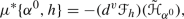  (4.14)

  where is the extended Hamiltonian density associated with h and is the vertical differential of . So, we have

  $$\begin{aligned} \{\alpha ^0, h\} = -\langle \sharp (d\alpha ^0), dh \rangle . \end{aligned}$$

  (4.15)

• (ii) If 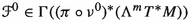then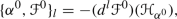

  

  (4.16)

  where is the linear part of the differential of .

Remark 4.6

Note that $\{\alpha ^0, h\} \in \Gamma ((\pi \circ \nu ^0)^*(\Lambda ^mT^*M))$ and, thus, $\mu ^*\{\alpha ^0, h\} \in \Gamma ((\pi \circ \nu )^*(\Lambda ^mT^*M))$. In fact,

Proof of Theorem 4.3

It is clear that is a linear map. So, we must prove that is a Lie algebra morphism. For this purpose, we will use Lemmas 4.4 and 4.5.

If $\alpha ^0, \beta ^0$ are currents and $h \in \Gamma (\mu )$ is a Hamiltonian section then, using (4.12) and (4.14), we obtain

Therefore, from Lemma 4.4, it follows that

Now, using (4.14) and the fact the vector fields and are $\mu$-projectable on the vector fields and , respectively, we deduce

So, from (4.16), we obtain that

Finally, using (4.12) and the fact that

we conclude that

which proves the result. $\square$

Proof of Lemma 4.4

It is clear that the map is linear. So, we will prove that

for .

Now, we have that

Thus, using (4.3) and the fact that is closed, we deduce that

But, since the vector field on is $\mu$-projectable over the vector field on , it follows that

Therefore, using (4.7), we obtain that

So, from (4.3), it follows that

and, since is non-degenerate, this implies the result. $\square$

Proof of Lemma 4.5

Suppose that

$$\begin{aligned} \alpha ^0(x^{i}, u^{\alpha }, p_\alpha ^{i}) = \left( Y^\alpha (x, u)p_\alpha ^{i} + \alpha ^{i}(x, u)\right) d^{m-1}x_i. \end{aligned}$$

(i) If

$$\begin{aligned} h(x^{i}, u^{\alpha }, p_\alpha ^{i}) = (x^{i}, u^{\alpha }, -H(x^{j}, u^\beta , p_\beta ^j), p_\alpha ^{i}) \end{aligned}$$

then, from (3.2) and (4.5), we have

This, by (3.40), implies

Finally, using (4.14), Definition 3.3, and the fact that is $\mu$-projectable on the vector field , we deduce that (4.15) also holds.

(ii) Suppose that

Then, we have

Thus, using (4.6), it follows

Therefore, from (3.41), we deduce the result. $\square$

5 Examples

5.1 Time-dependent Hamiltonian mechanics

In this section, we will use the following terminology. Let $\tau : V \rightarrow P$ be a vector bundle. Then, we can consider the vector bundle

$$\begin{aligned} id_{\mathbb {R}} \times \tau : \mathbb {R} \times V \rightarrow \mathbb {R} \times P. \end{aligned}$$

The sections of this vector bundle are just the time-dependent sections of $\tau : V \rightarrow P$. For this reason, the vector bundle $id_{\mathbb {R}} \times \tau : \mathbb {R} \times V \rightarrow \mathbb {R} \times P$ will be called the time-dependent vector bundle associated with $\tau : V \rightarrow P$.

For time-dependent Mechanics, the base space of the configuration bundle is the real line $\mathbb {R}$, that is, we have a fibration $\pi :E \rightarrow \mathbb {R}$. This fibration is trivializable but not canonically trivializable. In fact, if one choses a reference frame one may trivialize the fibration. This means that E may be identified with a global product $\mathbb {R} \times Q$ and, under this identification, $\pi : E \simeq \mathbb {R} \times Q \rightarrow \mathbb {R}$ is the canonical projection on the first factor. For simplicity, in what follows, we will assume that this is our starting point although all the constructions in this section may be extended, in a natural way, if we don’t chose a reference frame (for an affine formulation of frame-independent Mechanics, we remit to [44,45,46,47, 51, 60].)

So, if the configuration bundle is trivial, the 1-jet bundle $J^1\pi = J^1(pr_1) \rightarrow E = \mathbb {R} \times Q$ may be identified with the affine subbundle of $T(\mathbb {R} \times Q) = \mathbb {R} \times \mathbb {R} \times TQ$

$$\begin{aligned} J^1(pr_1) = \left\{ \frac{\partial }{\partial t}_{|t} + v_q \in T_t\mathbb {R} \times T_qQ \mid (t, q) \in \mathbb {R} \times Q \text{ and } v_q \in T_qQ\right\} . \end{aligned}$$

Thus, $J^1(pr_1)$ is isomorphic to the vector bundle $\mathbb {R} \times TQ \rightarrow \mathbb {R} \times Q$.

An Ehresmann connection $^{H}: (\mathbb {R} \times Q) \times _\mathbb {R} T\mathbb {R} \rightarrow H \subseteq T(\mathbb {R} \times Q)$ on the fibration $pr_1: \mathbb {R} \times Q \rightarrow \mathbb {R}$ is completely determined by a vector field $\Gamma$ on $\mathbb {R} \times Q$ satisfying

$$\begin{aligned} \left\langle dt, \Gamma \right\rangle = 1. \end{aligned}$$

In fact, the horizontal subbundle associated with the connection is of rank 1 and generated by the vector field $\Gamma$.

The extended (resp. restricted) multimomentum bundle may be identified with the cotangent bundle $T^*(\mathbb {R} \times Q) = \mathbb {R} \times \mathbb {R} \times T^*Q$ (resp. the vector bundle $\mathbb {R} \times T^*Q$) and, under this identification, the multisymplectic structure on $\mathbb {R} \times \mathbb {R} \times T^*Q$ is just the canonical symplectic structure $\omega _{(\mathbb {R} \times Q)}$ on $\mathbb {R}\times \mathbb {R} \times T^*Q$.

We have a principal $\mathbb {R}$-action on $T^*(\mathbb {R} \times Q) = \mathbb {R} \times \mathbb {R} \times T^*Q$ given by

$$\begin{aligned} p' \cdot (t, p, \alpha _q) = (t, p+p', \alpha _q) \end{aligned}$$

for $(t, p, \alpha _q) \in \mathbb {R} \times T^*_qQ$ and $p' \in \mathbb {R}$. The principal bundle projection is just the canonical projection

$$\begin{aligned} \mu : T^*(\mathbb {R} \times Q) = \mathbb {R} \times \mathbb {R} \times T^*Q \rightarrow V^*(pr_1) = \mathbb {R} \times T^*Q, \; \; (t, p, \alpha _q) \rightarrow (t, \alpha _q). \end{aligned}$$

Note that $\mathbb {R} \times T^*Q$ admits a Poisson structure of corank 1 which is induced by the canonical symplectic structure on $T^*Q$. In fact, the $\mathbb {R}$-action on the extended multimomentum bundle preserves the symplectic form and the canonical projection $\mu$ is a Poisson map.

In this case, a Hamiltonian section $h: V^*(pr_1) = \mathbb {R} \times T^*Q \rightarrow T^*(\mathbb {R} \times Q) = \mathbb {R} \times \mathbb {R} \times T^*Q$ may be identified with a global time-dependent Hamiltonian function $H: \mathbb {R} \times T^*Q \rightarrow \mathbb {R}$. In addition, the couple

$$\begin{aligned} (\omega _h = h^*\omega _{(\mathbb {R} \times Q)}, \eta = (\pi \circ \nu ^0)^*(dt)) \end{aligned}$$

is a cosymplectic structure on $V^*(pr_1) = \mathbb {R} \times T^*Q$ and, thus, we can consider the Reeb vector field $\Gamma _H$ of $(\omega _H = \omega _h, \eta )$.

Remark 5.1

We recall that a cosymplectic structure on a manifold P of odd dimension $2p + 1$ is a couple $(\omega , \theta )$, where $\omega$ is a closed 2-form, $\theta$ is a closed 1-form and $\theta \wedge \omega ^p$ is a volume form on P. The Reeb vector field $\Gamma$ associated with the structure $(\omega , \theta )$ is the vector field on P which is completely characterized by the conditions

$$\begin{aligned} i_{\Gamma }\omega = 0, \quad i_{\Gamma }\eta = 1. \end{aligned}$$

Note that the 2-form $\omega _H$ on $\mathbb {R} \times T^*Q$ is given by

$$\begin{aligned} \omega _H = \omega _Q + dH \wedge dt, \end{aligned}$$

where $\omega _Q$ is the canonical symplectic structure on $T^*Q$. So, the Reeb vector field $\Gamma _H$ of the cosymplectic structure $(\omega _H, \eta )$ on $\mathbb {R} \times T^*Q$ is

$$\begin{aligned} (t, \alpha ) \rightarrow \Gamma _H(t, \alpha ) = \frac{\partial }{\partial t}_{|t} + X_{H(t, \cdot )}(\alpha ), \end{aligned}$$

with $X_{H(t, \cdot )}$ the Hamiltonian vector field on $T^*Q$ associated with the function

$$\begin{aligned} H(t, \cdot ): T^*Q \rightarrow \mathbb {R}, \; \; \beta \rightarrow H(t, \beta ). \end{aligned}$$

Thus, if $(t, q^{i}, p_{i})$ are canonical coordinates on $\mathbb {R} \times T^*Q$ then

$$\begin{aligned} \Gamma _H = \frac{\partial }{\partial t} + \sum _{i}\left( \frac{\partial H}{\partial p_i} \frac{\partial }{\partial q^{i}} - \frac{\partial H}{\partial q^{i}} \frac{\partial }{\partial p_{i}}\right) \end{aligned}$$

and the integral curves $t \rightarrow (t, q^{i}(t), p_{i}(t))$ of $\Gamma _H$ are just of the solution of the Hamilton equations for H, that is,

$$\begin{aligned} \displaystyle \frac{dq^{i}}{dt} = \frac{\partial H}{\partial p_i}, \; \; \; \frac{dp_{i}}{dt} = -\frac{\partial H}{\partial q^{i}}. \end{aligned}$$

Therefore, $\Gamma _H$ is the evolution vector field associated with the time-dependent Hamiltonian function $H: \mathbb {R} \times T^*Q \rightarrow \mathbb {R}$ (for more details see, for instance, [19, 24]).

In addition, the vector bundle $V^*(\pi \circ \nu )$ may be identified with the time-dependent cotangent bundle to $\mathbb {R} \times T^*Q$,

$$\begin{aligned} id_{\mathbb {R}} \times \pi _{\mathbb {R} \times T^*Q}: \mathbb {R} \times T^*(\mathbb {R} \times T^*Q) \rightarrow \mathbb {R} \times (\mathbb {R} \times T^*Q), \end{aligned}$$

where $\pi _{\mathbb {R} \times T^*Q}: T^*(\mathbb {R} \times T^*Q) \rightarrow \mathbb {R} \times T^*Q$ is the canonical projection.

Under the previous identification, the principal $\mathbb {R}$-action on $V^*(\pi \circ \nu ) \simeq \mathbb {R} \times T^*(\mathbb {R} \times T^*Q)\simeq \mathbb {R} \times (\mathbb {R} \times \mathbb {R} \times T^*T^*Q)$ is given by

$$\begin{aligned} p' \cdot (t,(p, p_q, \tilde{\gamma })) = (t,(p+p', p_q, \tilde{\gamma })), \end{aligned}$$

for $p' \in \mathbb {R}$ and $(t, (p, p_q,\tilde{\gamma })) \in \mathbb {R} \times ( \mathbb {R} \times \mathbb {R} \times T^*T^*Q)$.

Moreover, the extended phase bundle $\widetilde{\mathbb {P}(\pi )}$ is

$$\begin{aligned} \widetilde{\mathbb {P}(\pi )} = \{(t, dp_{|p} + \gamma ) \mid (t, p) \in \mathbb {R} \text{ and } \gamma \in T^*(T^*Q) \}. \end{aligned}$$

In other words, $\widetilde{\mathbb {P}(\pi )}$ may be identified with the time-dependent vector bundle associated with the vector bundle $id_{\mathbb {R}} \times \pi _{T^*Q}: \mathbb {R} \times T^*T^*Q \rightarrow \mathbb {R} \times T^*Q$, that is,

$$\begin{aligned} id_{\mathbb {R}} \times (id_{\mathbb {R}} \times \pi _{T^*Q}): \widetilde{\mathbb {P}(\pi )} \simeq \mathbb {R} \times (\mathbb {R} \times T^*T^*Q) \rightarrow T^*( \mathbb {R} \times Q)\simeq \mathbb {R} \times \mathbb {R} \times T^*Q \end{aligned}$$

and the principal $\mathbb {R}$-action on $\widetilde{\mathbb {P}(\pi )}\simeq \mathbb {R} \times (\mathbb {R} \times T^*T^*Q)$ is given by

$$\begin{aligned} p' \cdot (t, (p, \tilde{\gamma })) = (t, p+p' \tilde{\gamma }) \end{aligned}$$

for $p', t, p \in \mathbb {R}$ and $\tilde{\gamma } \in T^*(T^*Q)$.

Thus, the phase bundle $\mathbb {P}(\pi )$ may be identified with the time-dependent cotangent bundle to $T^*Q$

$$\begin{aligned} id_{\mathbb {R}} \times \pi _{T^*Q}: \mathbb {P}(\pi ) \simeq \mathbb {R} \times T^*T^*Q \rightarrow \mathbb {R} \times T^*Q. \end{aligned}$$

Then, the differential dh of h is just the vertical differential $d^vH$ (with respect to the projection $pr_1: \mathbb {R} \times T^*Q \rightarrow \mathbb {R}$) of the Hamiltonian function H, that is,

$$\begin{aligned} d^vH: \mathbb {R} \times T^*Q \rightarrow \mathbb {R} \times T^*T^*Q, \; \; (t, \alpha ) \rightarrow d^vH(t, \alpha ) = (t, dH_{(t, \cdot )}(\alpha )). \end{aligned}$$

On the other hand, the vector bundle L, which was introduced in Proposition 3.10, is isomorphic to the cotangent bundle to $\mathbb {R} \times T^*Q$.

Moreover, as we know, the 1-jet bundle to the projection

$$\begin{aligned} \pi \circ \nu ^0: \mathbb {R} \times T^*Q \rightarrow \mathbb {R} \end{aligned}$$

may be identified with the affine subbundle of $T(\mathbb {R} \times T^*Q)$ given by

$$\begin{aligned} \left\{ \frac{\partial }{\partial t}_{|t} + X_\alpha \in T_t \mathbb {R} \times T_\alpha T^*Q \mid (t, \alpha ) \in \mathbb {R} \times T^*Q\right\} \end{aligned}$$

(5.1)

or, equivalently, with the time-dependent tangent bundle to $T^*Q$

$$\begin{aligned} id_{\mathbb {R}} \times \tau _{T^*Q}: \mathbb {R} \times TT^*Q \rightarrow \mathbb {R} \times T^*Q. \end{aligned}$$

Under all the previous identifications, the affine bundle isomorphism $A: J^1(\pi \circ \nu ^0) \simeq \mathbb {R} \times TT^*Q \rightarrow \mathbb {P}(\pi ) \simeq \mathbb {R} \times T^*T^*Q$ is given by

$$\begin{aligned} A(t, X) = (t, i_X\omega _Q), \; \; \text{ for } (t, X) \in \mathbb {R} \times TT^*Q, \end{aligned}$$

with $\omega _Q$ the canonical symplectic structure of $T^*Q$. Thus, in this case, the vector subbundle ${\text {Ker}} A$ is trivial and this implies that there exists a unique Hamiltonian connection for the hamiltonian section h. In fact, the horizontal subbundle of such a connection is generated by the evolution vector field $\Gamma _H$.

In addition, if $\sharp ^\textrm{aff}: \mathbb {P}(\pi ) \rightarrow J^{1}(\pi \circ \nu ^0)$ is the inverse morphism of $A: J^{1}(\pi \circ \nu ^0) \rightarrow \mathbb {P}(\pi )$ it is clear that, under the identification of $J^1(\pi \circ \nu ^0)$ with the affine subbundle of $T(\mathbb {R} \times T^*Q)$ given by (5.1), the image of the section dh of $\mathbb {P}(\pi )$ is just the evolution vector field $\Gamma _H$.

On the other hand, the space of currents is the set of smooth real functions on $\mathbb {R} \times T^*Q$ (the space of observables in Classical Mechanics)

and it is clear that the space $\Gamma (\mu )$ of sections of the projection

$$\begin{aligned} \mu : T^*(\mathbb {R} \times Q) \rightarrow \mathbb {R} \times T^*Q \end{aligned}$$

may be also identified with $C^{\infty }(\mathbb {R} \times T^*Q)$. Then, the linear-affine bracket

is given by

$$\begin{aligned} \{F^0, H\} = \langle dF^0,\Gamma _H\rangle = \frac{\partial F^0}{\partial t} + \sum _{i}\left( \frac{\partial F^0}{\partial q^{i}} \frac{\partial H}{\partial p_i} - \frac{\partial F^0}{\partial p_{i}} \frac{\partial H}{\partial q^i} \right) , \end{aligned}$$

for .

This bracket was considered in [44, 45, 60].

In addition, the bracket on the space of observables is just the standard Poisson bracket $\{\cdot , \cdot \}_{\mathbb {R} \times T^*Q}$ induced by the canonical symplectic structure of $T^*Q$. In other words,

$$\begin{aligned} \{F^0, G^0\}_{\mathbb {R} \times T^*Q} = \sum _{i}\left( \frac{\partial F^0}{\partial q^{i}} \frac{\partial G^0}{\partial p_i} - \frac{\partial F^0}{\partial p_{i}} \frac{\partial G^0}{\partial q^i} \right) \end{aligned}$$

for $F^0, G^0 \in C^{\infty }(\mathbb {R} \times T^*Q)$.

Finally, the affine representation of the Lie algebra $(C^{\infty }(\mathbb {R} \times T^*Q), \{\cdot , \cdot \}_{\mathbb {R} \times T^*Q})$ on the affine space $\Gamma (\mu ) \simeq C^{\infty }(\mathbb {R} \times T^*Q)$ is given by

Concretely, we have

$$\begin{aligned} \{\{F_0, G_0\}_{\mathbb {R} \times T^*Q}, H\}=\{F_0, \{G_0, H\}\}_{\mathbb {R} \times T^*Q}- \{G_0, \{F_0, H\}\}_{\mathbb {R} \times T^*Q}. \end{aligned}$$

5.2 A particular case: the configuration bundle is trivial and the base space is orientable

In this section we will assume that $E = M \times Q$, $\pi : E \rightarrow M$ is the canonical projection $pr_1: M \times Q \rightarrow M$ on the first factor. In this case, the affine bundle

$$\begin{aligned} J^1(pr_1) \rightarrow M \times Q \end{aligned}$$

can be identified with the vector bundle

$$\begin{aligned} T^*M \otimes TQ = \cup _{(x, y) \in M \times Q}\textrm{Lin}(T_xM, T_yQ). \end{aligned}$$

Let us further assume that M is orientable, with $m = dim M \ge 2$, and fix a volume form $\text{ vol } \in \Omega ^m(M)$ on M. We denote by $\chi _{\text{ vol }}$ the m-vector on M which is characterized by the condition

$$\begin{aligned} i(\chi _{\text{ vol }})\text{ vol } = 1. \end{aligned}$$

Using the volume form $\text{ vol }$ on M, we have

$$\begin{aligned} \Lambda ^mT_x^*M \simeq \mathbb {R}, \;\; \; \forall x \in M, \end{aligned}$$

and the vector bundle $\Lambda ^mT^*M \rightarrow M$ may be trivialized as the trivial line vector bundle $M \times \mathbb {R} \rightarrow M$. Using $\text{ vol }$ again, the reduced multimomentun bundle is isomorphic to the vector bundle.

$$\begin{aligned} \Lambda ^{m-1}T^*M \otimes T^*Q = \cup _{(x, y) \in M \times Q}\textrm{Lin}(T_yQ, \Lambda ^{m-1}(T_x^*M)) \end{aligned}$$

We can also identify it with

$$\begin{aligned} TM \otimes T^*Q = \cup _{(x, y) \in M \times Q}{\text {Lin}} (T^*_{x}M, T^*_yQ ). \end{aligned}$$

As in the general case, we will denote by $\nu ^0: \Lambda ^{m-1}T^*M \otimes T^*Q \rightarrow M \times Q$ the vector bundle projection. We will see that this space admits a multisymplectic structure.

Proposition 5.2

Let be the m-form on given by

for $\gamma ^0 \in \textrm{Lin}(T_yQ, \Lambda ^{m-1}(T_x^*M))$ and $Z_1^0, \ldots , Z_m^0 \in T_{\gamma ^0}(\Lambda ^{m-1}T^*M \otimes T^*Q)$, where $pr_2: M \times Q \rightarrow Q$ is the projection on the second factor. Then, is a multisymplectic structure on .

Proof

A direct computation proves that the local expression of is

Thus, the local expression of is

(5.2)

Therefore,

which implies that is a multisymplectic structure on . $\square$

On the other hand, the extended multimomentum bundle may be identified with the Withney sum of the vector bundles $\Lambda ^mT^*M \times Q \rightarrow M \times Q$ and $\Lambda ^{m-1}T^*M \otimes T^*Q \rightarrow M \times Q$, that is,

So, using the volume form $\text{ vol }$, we deduce that

Under this identification, the canonical multisymplectic structure on is

where p is the canonical coordinate on $\mathbb {R}$. Here, we also denote by and $\text{ vol }$ the pullbacks to of and $\text{ vol }$, respectively.

Moreover, a Hamiltonian section is just a global Hamiltonian function on and the $(m+1)$-form $\omega _h$ on is

(5.3)

On the other hand, under the identification between and and using (B.1) (see Appendix B), it follows that

$$\begin{aligned} (\text{ vol})^\textbf{v} = \frac{\partial }{\partial p}, \end{aligned}$$

(5.4)

where p is the standard coordinate on $\mathbb {R}$.

So, the extended phase bundle $\widetilde{\mathbb {P}(pr_1)}$ is isomorphic to the affine bundle over

where $V(pr_1 \circ \nu )$ is the vertical bundle of the fibration .

Now, using the previous identifications, we have that the fibred action of $\pi ^*(\Lambda ^mT^*M)$ on is just the standard action of $\mathbb {R}$ on . Therefore, since

$$\begin{aligned} V_{(p, \gamma ^0)}(pr_1 \circ \nu ) \simeq \textrm{span}\frac{\partial }{\partial p}_{|p} \oplus V_{\gamma ^0}(pr_1 \circ \nu ^0), \end{aligned}$$

for , we deduce that the phase bundle $\mathbb {P}(pr_1)$ is isomorphic to the vector bundle $V^*(pr_1 \circ \nu ^0)$. An isomorphism

$$\begin{aligned} V^*(pr_1 \circ \nu ^0) \rightarrow \mathbb {P}(pr_1) = \frac{\widetilde{\mathbb {P}(pr_1)}}{\mathbb {R}} \end{aligned}$$

between these spaces is given by

for , with p an arbitrary real number.

Thus, the image of the vertical differential $d^vH$ of H under the previous isomorphism is just the equivalence class induced by the vertical differential of the extended Hamiltonian density . This implies that, under the identification between $V^*(pr_1 \circ \nu ^0)$ and $\mathbb {P}(pr_1)$, the differential dh of h (as a section of the affine bundle ) is just $d^vH$ (as a section of the vector bundle ).

Next, following Sect. 3.2 (see (3.14) and (3.15)), we will define the vector bundle monomorphism

as follows

for $U \in V_{\gamma ^0}(pr_1 \circ \nu ^0)$ and . We have

$$\begin{aligned} \flat ^0\left( \frac{\partial }{\partial u^\alpha }\right) = -(dp_\alpha ^{i} \wedge d^{m-1}x_i), \; \; \flat ^0\left( \frac{\partial }{\partial p_\alpha ^{i}}\right) = du^\alpha \wedge d^{m-1}x_i. \end{aligned}$$

Now, we consider the restriction to $J^1(pr_1 \circ \nu ^0)$ of the dual morphism of $\flat ^0$, that is,

$$\begin{aligned} (\flat ^0)^*: J^{1}(pr_1 \circ \nu ^0) \rightarrow V^*(pr_1 \circ \nu ^0). \end{aligned}$$

A direct computation proves that

for and . Thus, if $(x^{i}, u^\alpha , p_\alpha ^{i})$ are local coordinates on such that

$$\begin{aligned} \text{ vol } = d^mx \end{aligned}$$

then, using (5.2), we deduce that

$$\begin{aligned} (\flat ^0)^*(x^{i}, u^{\alpha }, p_\alpha ^{i}; u^\alpha _j, p^{i}_{\alpha j}) = \left( x^{i}, u^{\alpha }, p_\alpha ^{i}; -\sum _i p^{i}_{\alpha i}, u^\alpha _i\right) . \end{aligned}$$

This, from (3.20) and under the identification between $\mathbb {P}(\textrm{pr}_1)$ and $V^*(pr_1 \circ \nu ^0)$, implies that $(\flat ^0)^* = A$, with $A: J^{1}(pr_1 \circ \nu ^0) \rightarrow \mathbb {P}(pr_1)$ the affine bundle epimorphism given by (3.15), (3.18) and (3.19).

So, if $\widehat{(\flat ^0)^*}: J^{1}(pr_1 \circ \nu ^0)/ {\text {Ker}} A \rightarrow V^*(pr_1 \circ \nu ^0)$ is the affine bundle isomorphism induced by $(\flat ^0)^*: J^{1}(pr_1 \circ \nu ^0) \rightarrow V^*(pr_1 \circ \nu ^0)$ then, under the identification between $\mathbb {P}(pr_1)$ and $V^*(pr_1 \circ \nu ^0)$, we conclude that

$$\begin{aligned} \widehat{(\flat ^0)^*} = \hat{A}. \end{aligned}$$

We will denote by

$$\begin{aligned} \sharp ^0: V^*(pr_1 \circ \nu ^0) \rightarrow J^{1}(pr_1 \circ \nu ^0)/{\text {Ker}} A \end{aligned}$$

the inverse morphism of $\widehat{(\flat ^0)^*}: J^{1}(pr_1 \circ \nu ^0)/{\text {Ker}} A \rightarrow V^*(pr_1 \circ \nu ^0)$.

Now, from (5.3) and Definition 3.5, we deduce that a connection on the fibration is Hamiltonian if and only if

where $d^vH$ is the vertical differential of H with respect to the projection $pr_1 \circ \nu ^0$.

Moreover, using that $(\flat ^0)^* = A$, it follows that the vector subbundle L of introduced in Proposition 3.10 is

In addition, as we know (see first step in Sect. 3.4), we have that

$$\begin{aligned} \left( J^{1}(pr_1 \circ \nu ^0)/{\text {Ker}} A\right) ^+ = \textrm{Aff}\left( J^{1}(pr_1 \circ \nu ^0)/{\text {Ker}} A, \mathbb {R}\right) \simeq L. \end{aligned}$$

On the other hand, under the identification between and , the projection is just the canonical projection on the second factor. Thus, the affine space $\Gamma (\mu )$ is isomorphic to the vector space and the linear-affine bracket

given by (3.39) may be considered as a bracket

defined by

5.3 Continuum mechanics

In this section we develop the formulation of Continuum Mechanics as a Canonical Hamiltonian Field Theory. This covers the case of fluid mechanics and nonlinear elasticity. We shall assume that the reference configuration of the continuum is described by a manifold B of dimension N, $N=2,3$ possibly with boundary, and we suppose that the continuum evolves in a N dimensional manifold Q without boundary, the ambient manifold, typically $\mathbb {R} ^N$. The elements $x\in B$ denote the labels of the material points of the continuum, whereas the elements $u\in Q$ denote the current positions of these material points. The evolution of the continuum is described by a map $\varphi : [0,T]\times B \rightarrow Q$, where [0, T] is the interval of time. Hence, $u=\varphi (t,x)$ describes the position of the material point x at time t. We shall assume that for each t fixed, the map $x\in B \mapsto \varphi (t,x)\in Q$ is a smooth embedding. Boundary conditions will be described in Sect. 5.3.4.

5.3.1 Lagrangian and Hamiltonian formulations in continuum mechanics

Continuum mechanics is usually written either as a Lagrangian field theory or as an infinite dimensional classical Lagrangian or Hamiltonian system. While the infinite dimensional description is more classical, the field-theoretic description is especially useful for the derivation of multisymplectic integrators for fluid and elasticity [20,21,22, 55, 58].

In the field theoretic Lagrangian description, the map $\varphi$ is interpreted as a section $\phi \in \Gamma (\pi )$ of the trivial fiber bundle $\pi : E=M \times Q \rightarrow M$, $M=[0,T]\times B$, by writing $\phi (t,x)= (t,x, \varphi (t,x))$. The equations of motion are given by the Euler–Lagrange equations for a given Lagrangian density , $m=N+1$. Since the bundle is trivial, we have $J^1\pi _{(t,x,u)} \simeq T_{(t,x)}^*M \otimes T_{u}Q$. We denote by $(t,x^i, u^\alpha , V^\alpha , F^\alpha _i)$ the local coordinates. Writing locally the Lagrangian density as , the Euler–Lagrange equations are given by

In the infinite dimensional classical Lagrangian description, the map $\varphi$ is interpreted as a curve $\varphi (t)$ in the infinite dimensional manifold ${\text {Emb}}(B,Q)$ of smooth embeddings of B into Q. The equations are given by the (classical) Euler–Lagrange equations for the Lagrangian function $L:T {\text {Emb}}(B,Q)\rightarrow \mathbb {R}$ defined from as

where we assumed that the Lagrangian density does not depend explicitly on the time t, and $T_X\varphi :T_XB \rightarrow T_{\varphi (X)} Q$ denotes the tangent map to $\varphi \in {\text {Emb}}(B,M)$, i.e. locally $T_x\varphi = \varphi ^\alpha _{,i} \frac{\partial }{\partial u^\alpha }\otimes dx^i$. When L is hyperregular, to this classical Lagrangian description is formally associated a classical Hamiltonian description with respect to the Hamiltonian $H:T^*{\text {Emb}}(B,Q)\rightarrow \mathbb {R}$ defined on the (regular) cotangent bundle of ${\text {Emb}}(B,Q)$. The Hamiltonian is defined by

where $V\in T_\varphi {\text {Emb}}(B,Q)$ is such that . In this case, the associated equations can formally be written $\dot{F}=\{F,H\}_\textrm{can}$ with respect to the canonical Poisson bracket on $T^*{\text {Emb}}(B,Q)$.

The Hamiltonian formulation that we present below is different from this one, since it is associated to the field theoretic Lagrangian formulation. Roughly speaking, while the canonical Hamiltonian formulation recalled above is based on a Legendre transform with respect to the time direction only, the canonical Hamiltonian field theoretic description that we will describe below is based on a Legendre transform with respect to all the variables in the base manifold M.

We warn the reader that the coordinates $x^i$ that were used in the previous sections for the base manifold M are here given by $(t,x^i)$ for $M=[0,T]\times B$. The coordinates $u^\alpha _i$ used earlier on the fiber of $J^1\pi$ are here given by $(V^\alpha , F^\alpha _i)$ and represent the material velocity and the deformation gradient of the continuum.

5.3.2 Lagrangian density and Legendre transform

The Lagrangian density of continuum mechanics is defined with the help of given tensor fields on B and Q. In order to treat both fluid dynamics and elasticity from a unified perspective, we shall consider here a Riemannian metric G on B, two volume forms $\varrho$ and $\varsigma$ on B, and a Riemannian metric g on Q. Additional tensor fields can be introduced to describe electromagnetic effects or microstructures. The volume forms $\varrho$ and $\varsigma$ are the mass density and the entropy density in the reference configuration and are locally written as $\varrho ={\bar{\varrho }} d^NX$ and $\varsigma ={\bar{\varsigma }} d^NX$. The potential energy density is a bundle map

covering the projection $B\times Q\rightarrow B$. In local coordinates, it reads

This is a general form of potential energy density for continua, including fluid and elasticity, which may describe both internal and stored energies.

The associated Lagrangian density is given by the kinetic minus the potential energy, and reads

(5.5)

in local coordinates. Note that the Lagrangian is defined with the help of the given tensor fields $\varrho ={\bar{\varrho }} d^Nx$, $\varsigma ={\bar{\varsigma }} d^Nx$, $G^{-1}= G^{ij} \frac{\partial }{\partial x^i} \frac{\partial }{\partial x^j}$, and $g=g_{\alpha \beta } dx^\alpha dx^\beta$. We chose to work with the cometric $G^{ij}$ associated to $G_{ij}$, in order to directly get the Finger deformation (or left Cauchy–Green) tensor $b^{\alpha \beta }$, rather than its inverse, later.

The restricted multimomentum bundle for continuum mechanics is given by

with coordinates $(t,x^i, u^\alpha , M_\alpha , P^i_\alpha )$. The restricted Legendre transform of the Lagrangian density is

(5.6)

with $M_\alpha$ and $P^i_\alpha$ given by

(5.7)

with $M_\alpha$ the momentum density (in the Lagrangian description) and $P^i_\alpha$ is the Piola–Kirchoff stress tensor density. Note that the coordinates $(M_ \alpha , P_ \alpha ^i)$ on the fiber of correspond to the coordinates denoted $p_ \alpha ^i$ earlier.

The Eulerian versions of these tensor densities are the Eulerian momentum density $m_\alpha$ and the Cauchy stress tensor density $\sigma ^{\alpha \beta }$ given by the Piola transformation

$$\begin{aligned} m_\alpha = M_\alpha {\text {det}}(F)^{-1}\quad \text {and}\quad \sigma ^{\alpha \beta }=- F_i^\alpha P_\gamma ^i g^{\beta \gamma }{\text {det}}(F)^{-1}. \end{aligned}$$

(5.8)

From the second relation, we have

$$\begin{aligned} P_\alpha ^i = - {\text {det}}(F) ( F ^{-1} )_\gamma ^i \sigma ^{\gamma \beta } g_{\beta \alpha }. \end{aligned}$$

(5.9)

Note that the first relation in (5.7) is always invertible, but the invertibility of the second relation depends in the potential energy density . As we shall illustrate below, relation (5.9) is extremely useful to check if the restricted Legendre transform (5.6) is an isomorphism, in which case we say that the Lagrangian density is hyperregular.

5.3.3 The Hamiltonian density and the linear-affine bracket for continuum mechanics

By assuming that is hyperregular, we get the Hamiltonian

(5.10)

where $F_i^\alpha$ is expressed in terms of the variables in by inverting the second relation in (5.7).

A section of the restricted momentum bundle is locally given by

$$\begin{aligned} s_0(t,x^i )= \left( t, x^i, \varphi ^\alpha (t, x^i ), M_\alpha (t,x^i),P_\alpha ^i (t,x^i ) \right) \end{aligned}$$

and, in the hyperregular case, the Euler–Lagrange equation are equivalent to the Hamilton–deDonder–Weyl equations given by

$$\begin{aligned} \frac{\partial \varphi ^\alpha }{\partial t }= \frac{\partial H}{\partial M_\alpha }, \quad \frac{\partial \varphi ^\alpha }{\partial x^i }= \frac{\partial H}{\partial P_\alpha ^i },\quad \frac{\partial M_\alpha }{\partial t} + \frac{\partial P _\alpha ^i }{\partial x^i }= -\frac{\partial H}{\partial u ^\alpha }. \end{aligned}$$

(5.11)

These equations admit the canonical linear-affine bracket formulation, that is, a section $(t, x^{i}) \rightarrow s^0(t, x^{i}) = (t, x^{i}, u^\alpha (t, x), M_\alpha (t, x), P_\alpha ^{i}(t, x))$ is a solution of the previous equations if

(5.12)

where the currents for Continuum Mechanics are of the form

$$\begin{aligned}&\alpha ^0(t,x ^i, u^\alpha , M_\alpha , P^i_\alpha )\\&\quad = \alpha ^{00}(t,x ^i, u^\alpha , M_\alpha , P^i_\alpha )d^Nx - \alpha ^{0i}(t,x ^i, u^\alpha , M_\alpha , P^i_\alpha )dt \wedge d^{N-1}x_i\\&\quad = \big (Y^\alpha (t,x,u) M_\alpha + \beta ^0(t,x,u) \big ) d^Nx -\big (Y^\alpha (t,x,u) P^i_\alpha + \beta ^i(t,x,u) \big ) dt \wedge d^{N-1}x_i \end{aligned}$$

with $d^{N-1}x_i= i_{\frac{\partial }{\partial x^i} } d^Nx$. The canonical linear-affine bracket is given by

$$\begin{aligned} \begin{array}{l} \displaystyle \{\alpha ^{00} d^Nx - \alpha ^{0i}dt \wedge d^{N-1}x_i, H \} \\ \qquad \displaystyle = \frac{\partial \alpha ^{00} }{\partial t} + \frac{\partial \alpha ^{0i} }{\partial x^i}+ \frac{\partial \alpha ^{00}}{\partial u^ \alpha } \frac{\partial H}{\partial M_\alpha }- \frac{1}{m} \frac{\partial H}{\partial u^\alpha } \frac{\partial \alpha ^{00} }{\partial M_ \alpha } + \frac{\partial \alpha ^{0i}}{\partial u^ \alpha } \frac{\partial H}{\partial P^i_ \alpha } - \frac{1}{m} \frac{\partial H}{\partial u^\alpha } \frac{\partial \alpha ^{0i} }{\partial P_ \alpha ^i}. \end{array} \end{aligned}$$

This formulation assumes that the Legendre transform is invertible. Except in some simple situations, this invertibility is a priori difficult to check. We shall show below how to facilitate the approach by using two symmetries of the potential energy density . The first one, the material covariance, is related to the isotropy of the continuum, while the second, the material frame indifference, is a general covariance assumption of continuum theories, see [38, 39, 61].

We assume that the potential energy density is of the form

where ${\bar{\epsilon }}$ is the potential energy density in the Eulerian description. This assumption is compatible with the assumption of material covariance. Here $\epsilon ={\bar{\epsilon }} d^Nu$ is a bundle map

$$\begin{aligned} \epsilon : \Lambda ^NT^*_u Q \times \Lambda ^NT^*_u Q \times S^2 T_xQ \times S^2 T_x^*Q\rightarrow \Lambda ^N_u Q \end{aligned}$$

covering the identity on Q. From this expression, we compute the momenta from the second equality in (5.7) as

$$\begin{aligned} \begin{aligned} P_\alpha ^i =\left( \Big ({\bar{\epsilon }} -\frac{\partial {\bar{\epsilon }} }{\partial {\bar{\rho }} } {\bar{\rho }} - \frac{\partial {\bar{\epsilon }} }{\partial {\bar{s}} } {\bar{s}} \Big ) (F ^{-1} )_\alpha ^i + 2\frac{\partial {\bar{\epsilon }} }{\partial b^{\alpha \beta }}F_i ^\gamma G^{ij} F_j ^\beta ( F ^{-1} )_\gamma ^i \right) {\text {det}}(F), \end{aligned} \end{aligned}$$

(5.13)

where we introduced the notations

$$\begin{aligned} {\bar{\rho }} = {\bar{\varrho }}{\text {det}}(F)^{-1},\quad {\bar{s}} ={\bar{\varsigma }}{\text {det}}(F)^{-1},\quad b^{\alpha \beta }=F^\alpha _i G^{ij} F_j^\beta . \end{aligned}$$

These are the local expressions of the mass density and entropy density in Eulerian description, and of the Finger deformation (or left Cauchy–Green) tensor.

The associated Cauchy stress tensor density $\sigma$, see the second equation in (5.8), is

$$\begin{aligned} \sigma ^{\alpha \beta } = \Big ({\bar{\epsilon }} -\frac{\partial {\bar{\epsilon }} }{\partial {\bar{\rho }} } {\bar{\rho }} - \frac{\partial {\bar{\epsilon }} }{\partial {\bar{s}} } {\bar{s}} \Big ) g^{\alpha \beta } + 2\frac{\partial {\bar{\epsilon }} }{\partial b^{\gamma \delta }}F_i ^\alpha G^{ij} F_j ^\delta g^{\gamma \beta }. \end{aligned}$$

(5.14)

If in addition satisfies the material frame indifference, then

$$\begin{aligned} \epsilon (\psi ^*\rho , \psi ^* s, \psi ^* b, \psi ^*g)= \psi ^*\big (\epsilon (\rho ,s,b,g)\big ), \end{aligned}$$

(5.15)

for all diffeomorphisms $\psi$ of Q and we have the Doyle–Ericksen formula

$$\begin{aligned} \sigma ^{\alpha \beta }= 2\frac{\partial {\bar{\epsilon }} }{\partial g_{\alpha \beta }}. \end{aligned}$$

(5.16)

By inserting these relations into (5.10), we get the following result which is a step towards a more explicit expression of the Hamiltonian density, because in practice $\epsilon$, rather than , is given.

Proposition 5.3

Assume that the Lagrangian is hyperregular and that satisfies the two invariance mentioned above, and consider the associated Eulerian potential energy density $\epsilon$. Then, the Hamiltonian density of continuum mechanics is given by

$$\begin{aligned} H(t,x^i,u^\alpha , M_\alpha , P_\alpha ^i)=\frac{1}{2} g^{\alpha \beta }(u)M_\alpha M_\beta \frac{1}{ {\bar{\varrho }} (x)}+\left( {\bar{\epsilon }} - 2\frac{\partial {\bar{\epsilon }} }{\partial g_{\alpha \beta } }g_{\alpha \beta }(u) \right) {\text {det}}(F).\nonumber \\ \end{aligned}$$

(5.17)

5.3.4 Boundary conditions

We briefly describe two mains boundary conditions used in Continuum Mechanics following Sect. 3.6. These conditions only arise at the spatial part of the boundary of the base manifold M, hence the bundle $B_0$ is over $[0,T] \times \partial B \subset \partial M$ only and the boundary condition reads $s( [0,T] \times \partial B) \subseteq B_0$.

For a continuum moving in a fixed domain $B' \subset Q$ diffeomorphic to B, we have the boundary condition $\varphi (t, \partial B)= \partial B'$ on the motion and, in addition, the boundary condition on the Piola–Kirchhoff stress tensor P given by $P_ \alpha ^i(t,x) N^\flat _i(x)|_{TB'}=0$, for all $x \in \partial B$, with N the normal vector field to B with respect to G. This corresponds to zero tangential traction on the boundary, a condition that vanishes for fluids. In this case, the subbundle $B^0 \rightarrow [0,T] \times \partial B$ is given by

$$\begin{aligned} B^0(t,x^i)= \{ (t,x^i,u^ \alpha , M_ \alpha , P_ \alpha ^i) \mid u^ \alpha \in \partial B', \;P_ \alpha ^i N_i^\flat \in (TB')^\circ \}, \quad (t,x^i) \in [0,T] \times \partial B. \end{aligned}$$

In particular, we have $B_E^0 = [0,T] \times \partial B \times \partial B'$ and $B_0 \rightarrow B_E^0$ is a vector bundle.

For a free boundary continuum we take

$$\begin{aligned} B^0(t,x^i)= \{ (t,x^i,u^ \alpha , M_ \alpha , P_ \alpha ^i) \mid P_ \alpha ^i N_i^\flat =0\}, \quad (t,x^i) \in [0,T] \times \partial B, \end{aligned}$$

which corresponds to zero traction on the boundary. This reduces to zero pressure at the boundary for fluids. We have $B_E^0 = [0,T] \times \partial B \times Q= E|_{ [0,T] \times \partial B}$ and $B_0 \rightarrow B_E^0$ again is a vector bundle.

5.3.5 Fluid dynamics

In this case the energy density $\epsilon$ only depends on the mass density and entropy density $\rho ={\bar{\rho }} d^Nu$ and $s={\bar{s}} d^Nu$, so the Cauchy stress density is given by

$$\begin{aligned} \sigma ^{\alpha \beta } = \Big ({\bar{\epsilon }} -\frac{\partial {\bar{\epsilon }} }{\partial {\bar{\rho }} } {\bar{\rho }} - \frac{\partial {\bar{\epsilon }} }{\partial {\bar{s}} } {\bar{s}} \Big ) g^{\alpha \beta }= - p({\bar{\rho }}, {\bar{s}},g_{\alpha \beta })\sqrt{\det g} g^{\alpha \beta }, \end{aligned}$$

see (5.14), where p is the pressure of the fluid. In this case (5.9) yields

$$\begin{aligned} P^i_\alpha = {\text {det}}(F) (F^{-1})^i_\alpha p \big ({\bar{\varrho }}{\text {det}}(F)^{-1},{\bar{\varsigma }} {\text {det}}(F)^{-1},g_{\alpha \beta }\big ) \sqrt{\det g}. \end{aligned}$$

This relation is of the form

$$\begin{aligned} P^i_\alpha = \textsf {f}( {\text {det}}(F)) (F^{-1})^i_\alpha , \end{aligned}$$

(5.18)

for some function $\textsf {f}$. If the function $x\mapsto {\textsf {f}(x)^N}{x}$ is invertible on $]0,\infty [$, with inverse $\textsf {g}$, then relation (5.18) is invertible, with inverse

$$\begin{aligned} F^\alpha _i = \textsf {f}(\textsf {g}^{-1}({\text {det}}(P))) (P^{-1})^\alpha _i. \end{aligned}$$

(5.19)

In this case the Lagrangian density is hyperregular. Note that the function $\textsf {f}$, and hence the hyperregularity, depends on the state function of the fluid, i.e., the relation $\epsilon =\epsilon (\rho , s, g)$.

Hyperregularity is satisfied for a large class of state equations, including the important case of a perfect gas for which $\epsilon (\rho , s, g)=\epsilon _0 e^{\frac{1}{C_v}\left( \frac{s}{\rho }- \frac{s_0}{\rho _0}\right) }\big (\frac{\rho }{\rho _0\mu (g)}\big )^{\gamma }\mu (g)$, where $\gamma = C_p/C_v$ is the adiabatic index and $\mu (g)$ is the volume form associated to g, i.e. $\mu (g)= \sqrt{\det g}d^Nu$. In this case, we compute the pressure as $p\sqrt{\det g}= (\gamma - 1){\bar{\epsilon }}$.

Note that, as it should, $\epsilon$ satisfies (5.14). Computing the derivative of ${\bar{\epsilon }}$ with respect to the Riemannian metric, we get

$$\begin{aligned} \frac{\partial {\bar{\epsilon }} }{\partial g_{\alpha \beta }}= \frac{1}{2} (1- \gamma ){\bar{\epsilon }} g^{\alpha \beta }, \end{aligned}$$

so one directly checks that the Doyle–Ericksen formula (5.16) is verified.

For fluids, the Hamiltonian density is

$$\begin{aligned} H(t,x^i,u^\alpha , M_\alpha , P_\alpha ^i)=\Big (\frac{1}{2} g^{\alpha \beta }(u)M_\alpha M_\beta \frac{1}{{\bar{\varrho }} (x)}+\Big ({\bar{\epsilon }} + N p \sqrt{\det g}\Big ){\text {det}}(F) \Big ) dt\wedge d^Nx, \end{aligned}$$

where ${\text {det}}(F)$ is found from (5.19). In particular, for the perfect gas, we have ${\bar{\epsilon }} + N p \sqrt{\det g}=(1+N(\gamma -1)){\bar{\epsilon }}$.

The fluid equations can thus be written in the canonical linear-affine bracket form (5.12).

5.3.6 Nonlinear elasticity

In general, the Hamiltonian density in nonlinear elasticity takes a complicate expression due to the dependence of $\epsilon$ on the Finger deformation tensor b.

For example, for the compressible neo-Hookean material (see [3, 64]), with $N=3$, the energy density is

$$\begin{aligned} \epsilon ( \rho , b, g)= \frac{1}{2} \kappa \left( \ln J \right) ^2 \rho + \frac{1}{2} \mu \left( J ^{-2/3} {\text {Tr}}_g(b)-3 \right) \rho , \qquad J:= \frac{ \mu (g)}{ \mu (b ^\flat )}, \end{aligned}$$

where $\kappa$ is the bulk modulus, $\mu$ is the Lamé constant, and $\mu (b^\flat )$ is the volume form associated to the Riemannian metric $b^\flat$, obtained by lowering the indices of b. One observes that (5.14) is satisfied. The Doyle–Ericksen formula yields the expression of the stress tensor density

$$\begin{aligned} \sigma = 2 \frac{\partial \epsilon }{\partial g}= \kappa (\ln J ) g^\sharp \rho + \mu J^{-2/3} \left( b- \frac{1}{3} {\text {Tr}}_g(b) g^\sharp \right) \rho . \end{aligned}$$

We thus get $2 \frac{\partial \epsilon }{\partial g}\!:\!g= 3 \kappa \ln J\rho$ which can then be inserted in (5.17) to yield the Hamiltonian density.

We shall illustrate the derivation of the Hamiltonian density by considering the simplified situation $\epsilon ( \rho ,b, g)= \frac{1}{2} {\text {Tr}}_g(b) \rho$. In this case $\sigma = b \rho$, so we get the momenta

$$\begin{aligned} P_\alpha ^i =- G^{ij} F_j ^\beta g_{\alpha \beta }{\bar{\varrho }}. \end{aligned}$$

Using this and $\sigma \!: \!g= {\text {Tr}}_g(b) \rho$, we get the Hamiltonian density

$$\begin{aligned} H(t,x^i,u ^\alpha , M_\alpha , P_\alpha ^i )= \left( \frac{1}{2} g^{\alpha \beta }(u)M_\alpha M_\beta \frac{1}{ \varrho _\textrm{loc}(x)}- \frac{1}{2} P_\alpha ^iG_{ij}P_\beta ^jg_{\alpha \beta } \frac{1}{\varrho _\textrm{loc}(x)}\right) dt\wedge d^3x. \end{aligned}$$

The nonlinear elasticity equations can thus be written in the canonical linear-affine bracket form (5.12).

5.4 Yang–Mills theory

Yang–Mills theory may be considered as a singular Lagrangian field theory of first order associated with a principal G-bundle over an oriented Riemannian (or a Lorentzian manifold) space M (possibly with boundary) of dimension m and where G is a compact Lie group of dimension n (we will follow [49]).

We will denote by g the metric on M. For simplicity, we will assume that the principal bundle is trivial, g is a Riemannian metric and $\partial M = \phi$.

Under the previous conditions, the configuration bundle of the theory is the vector bundle

$$\begin{aligned} \pi _{M, \mathfrak {g}}: E: =T^*M \otimes \mathfrak {g} \rightarrow M \end{aligned}$$

where $\mathfrak {g}$ is the Lie algebra of G.

Then, we will proceed as follows. We will introduce a Lagrangian density on the 1-jet bundle of the fibration $\pi _{M, \mathfrak {g}}: T^*M \otimes \mathfrak {g} \rightarrow M$. This Lagrangian density is singular. In fact, the image of the corresponding Legendre transformation is a proper submanifold of the restricted multimomentum bundle . Using the restricted and the extended Legendre transformation, we will construct a constrained Hamiltonian section of the fibration . Now, if we consider an (arbitrary) hamiltonian section , whose restriction to coincides with $h_1$, we will obtain a Hamiltonian field theory in such a way that the solutions of the Hamilton–deDonder–Weyl equations for h which are contained in are just the solutions of the corresponding Yang–Mills theory.

5.4.1 The Lagrangian formalism

Note that the sections of the vector bundle $\pi _{M, \mathfrak {g}}: T^*M \otimes \mathfrak {g} \rightarrow M$ are the principal connections on the trivial principal bundle $pr_1: M \times G \rightarrow M$. As we know, the 1-jet bundle $J^1 \pi _{M, \mathfrak {g}}$ is an affine bundle over $T^*M \otimes \mathfrak {g}$. The key point is that there is a canonical epimorphism off affine bundles (over the vector bundle projection $\pi _{M, \mathfrak {g} }: T^*M \otimes \mathfrak {g} \rightarrow M$), $F: J^1 \pi _{M, \mathfrak {g}} \rightarrow \Lambda ^2T^*M \otimes \mathfrak {g}$, which is characterized by the condition

$$\begin{aligned} F(j^1 \Theta (x))= \textrm{d} \Theta (x)+ [ \Theta (x), \Theta (x)], \; \; \text{ for } x\in M, \end{aligned}$$

for all principal connections $\Theta$. In other words, the image by F of the 1-jet bundle of a principal connection is just the curvature of the connection.

If $(x^{i})$ are local coordinates on M and $\{e_\alpha \}$ is a basis of $\mathfrak {g}$, we have the corresponding local coordinates $(x^{i}, u^\alpha _i)$ on E and $(x^{i}, u^\alpha _i, u^\alpha _{ij})$ on $J^1\pi _{M, \mathfrak {g}}$. Moreover,

$$\begin{aligned} F(x^{i}, u^\alpha _i, u^\alpha _{ij}) = \frac{1}{2} F_{kl}^\gamma (x^{i}, u^\alpha _i, u^\alpha _{ij})(dx^k \wedge dx^l) \otimes e_\gamma \end{aligned}$$

with

$$\begin{aligned} F_{kl}^\gamma (x^{i}, u^\alpha _i, u^\alpha _{ij}) = u^\gamma _{lk} - u^\gamma _{kl} + c_{\alpha \beta }^\gamma u^\alpha _k u^\beta _l. \end{aligned}$$

(5.20)

Here, $c_{\alpha \beta }^\gamma$ are the structure constants of the Lie algebra $\mathfrak {g}$ with respect to the basis $\{e_\gamma \}$.

Next, we will introduce the Lagrangian density

First of all, since the manifold M is oriented, the vector bundle $\pi _{M, \mathfrak {g}}^*(\Lambda ^mT^*M) \rightarrow E$ is the trivial line bundle $E \times \mathbb {R} \rightarrow E$. So, the Lagrangian density is, in fact, a real $C^\infty$-function $L: J^1\pi _{M, \mathfrak {g}} \rightarrow \mathbb {R}$.

In addition, we will fix an Ad-invariant scalar product $\langle \cdot , \cdot \rangle$ on $\mathfrak {g}$ (which is possible, since G is compact). Then, the scalar product on $\mathfrak {g}$ and the Riemannian metric on M induce a bundle metric on the vector bundle

$$\begin{aligned} pr_1: E \times _M \Lambda ^2T^*M \otimes \mathfrak {g} \rightarrow E. \end{aligned}$$

So, we can consider the real function $L: J^1\pi _{M, \mathfrak {g}} \rightarrow \mathbb {R}$ given by

$$\begin{aligned} L(z) = \displaystyle \frac{1}{4} \Vert F(z)\Vert ^2, \; \; \text{ for } z \in J^1\pi _{M, \mathfrak {g}}, \end{aligned}$$

where the norm is taken with respect to the bundle metric on the vector bundle $pr_1: E \times _M \Lambda ^2T^*M \otimes \mathfrak {g} \rightarrow E.$

The local expression of L is

$$\begin{aligned} L(x^{i}, u^\alpha _i, u^\alpha _{ij}) = \displaystyle \frac{1}{4} F_{kl}^\gamma (x^{i}, u^\alpha _i, u^\alpha _{ij}) F^{kl}_\gamma (x^{i}, u^\alpha _i, u^\alpha _{ij}) \end{aligned}$$

with

$$\begin{aligned} F^{kl}_\gamma = F_{mn}^\beta g^{km}g^{ln}\langle \cdot , \cdot \rangle _{\beta \gamma } \end{aligned}$$

and $(g_{ij})$ the matrix of the coefficients of g, $(g^{ij})$ the inverse matrix and

$$\begin{aligned} \langle \cdot , \cdot \rangle _{\beta \gamma } = \langle e_\beta , e_\gamma \rangle . \end{aligned}$$

Thus, the Euler–Lagrange equations for L

$$\begin{aligned} \displaystyle \frac{\partial }{\partial x^j}\left( \frac{\partial L}{\partial u^\alpha _{ij}}\right) - \displaystyle \frac{\partial L}{\partial u^\alpha _i} = 0, \; \; u^\alpha _{ij} = \displaystyle \frac{\partial u^\alpha _i}{\partial x^j} \end{aligned}$$

are, in this case, the well-known Yang–Mills equations

$$\begin{aligned} \displaystyle \sum _i \frac{\partial F^{ij}_\alpha }{\partial x^{i}} + c_{\alpha \beta }^\gamma u^\beta _i F^{ij}_\gamma =0, \; \; u^\alpha _{ij} = \displaystyle \frac{\partial u^\alpha _i}{\partial x^j}. \end{aligned}$$

(5.21)

5.4.2 The Legendre transformations and the constrained Hamiltonian formalism

First of all, we will consider the restricted Legendre transformation associated with L

Note that, since M is oriented, the restricted multimomentum bundle may be identified with the dual bundle $V^*(J^1\pi _{M,\mathfrak {g}})$ of $V(J^1\pi _{M,\mathfrak {g}})$. So,

The transformation $leg_L$ is given by

$$\begin{aligned} leg_L(z)(v) = \frac{d}{dt}_{|t=0} L(z + tv), \end{aligned}$$

for $z \in J^1_y\pi _{M, \mathfrak {g}}$, and $y \in E$. The local expression of $leg_l$ is

$$\begin{aligned} leg_L(x^{i}, u^\alpha _i, u^\alpha _{ij}) = \left( x^{i}, u^\alpha _i, \frac{\partial L}{\partial u^\alpha _{ij}}\right) = (x^{i}, u^\alpha _i, -F^{kl}_\gamma (x^{i}, u^\alpha _i, u^\alpha _{ij})). \end{aligned}$$

This implies that the image of $leg_L$ is the vector subbundle (over E) of

Thus, the map is a submersion with connected fibers and L is almost regular.

On the other hand, we can consider the extended Legendre transformation associated with L defined by

$$\begin{aligned} Leg_L(z)(z') = \displaystyle \frac{d}{dt}_{|t=0} L(z + t(z' -z)), \; \; \text{ for } z, z' \in J^1_y\pi _{M,\mathfrak {g}} \text{ and } y \in E. \end{aligned}$$

The local expression of $Leg_L$ is

$$\begin{aligned} Leg_L(x^{i}, u^\alpha _i, u^\alpha _{ij})= & {} \left( x^{i}, u^\alpha _i, -E_L(x^{i}, u^\alpha _i, u^\alpha _{ij}), \frac{\partial L}{\partial u^\beta _{kl}}\right) \\= & {} \left( x^{i}, u^\alpha _i, -E_L(x^{i}, u^\alpha _i, u^\alpha _{ij}), -F_{kl}^\beta (x^{i}, u^\alpha _i, u^\alpha _{ij})\right) , \end{aligned}$$

where

$$\begin{aligned} E_L(x^{i}, u^\alpha _i, u^\alpha _{ij}) = \displaystyle \frac{1}{4} F_{ij}^\alpha (x^{k}, u^\beta _k, u^\beta _{kl}) F^{ij}_\alpha (x^{k}, u^\beta _k, u^\beta _{kl}) - \displaystyle \frac{1}{2} c_{\alpha \beta }^\gamma u^\alpha _i u^\beta _j F^{ij}_\gamma (x^{k}, u^\beta _k, u^\beta _{kl}). \end{aligned}$$

Note that if is the canonical projection then the image of $Leg_L$ is a submanifold of which is diffeomorphic to , via the restriction of $\mu$ to . The following diagram illustrates the situation

The maps and are surjective submersions and, thus, we have a constrained Hamiltonian field theory. As a consequence (see, for instance, [25]), one may introduce a constrained Hamiltonian section

in such a way that

$$\begin{aligned} h_1 \circ leg_1 = Leg_1. \end{aligned}$$

In fact, . In addition, if $(x^{i}, u^\alpha _i, p, p_\alpha ^{ij})$ and $(x^{i}, u^\alpha _i, p_\alpha ^{ij})$ are the standard local coordinates on and , respectively, we can take local coordinates

$$\begin{aligned} (x^{i}, u^\alpha _i, p, \pi _\alpha ^{ij}) \; \text{ and } (x^{i}, u^\alpha _i, \pi _\alpha ^{ij}) \end{aligned}$$

on and , respectively, with

$$\begin{aligned} \frac{1}{2} \pi ^{ij}_\alpha = p^{ij}_\alpha , \; \; \text{ for } i < j. \end{aligned}$$

(5.22)

Then,

$$\begin{aligned} h_1(x^{i}, u^\alpha _i, \pi _\alpha ^{ij}) = (x^{i}, u^\alpha _i, -H_1(x^{i}, u^\alpha _i, \pi _\alpha ^{ij}), \pi _\alpha ^{ij}) \end{aligned}$$

where

$$\begin{aligned} H_1(x^{i}, u^\alpha _i, \pi _\alpha ^{ij}) = \displaystyle \frac{1}{4} p_{ij}^\alpha p^{ij}_\alpha + \displaystyle \frac{1}{2} c_{\alpha \beta }^\gamma u^\alpha _i u^\beta _j p^{ij}_\gamma = \displaystyle \frac{1}{16} \pi _{ij}^\alpha \pi ^{ij}_\alpha + \displaystyle \frac{1}{4} c_{\alpha \beta }^\gamma u^\alpha _i u^\beta _j \pi ^{ij}_\gamma . \end{aligned}$$

(5.23)

Note that we are assuming

$$\begin{aligned} \pi ^{ij}_\alpha = -\pi ^{ji}_\alpha \; \; \text{ if } i > j \; \; \text{ and } \pi ^{ii}_\alpha = 0. \end{aligned}$$

In addition,

$$\begin{aligned} \pi _{ij}^\alpha = \pi ^{kl}_\beta g_{ik}g_{jl} \langle \cdot , \cdot \rangle ^{\alpha \beta }. \end{aligned}$$

It is clear that

$$\begin{aligned} E_L= H_1 \circ leg_1. \end{aligned}$$

Moreover, on

$$\begin{aligned} - F^{ij}_\alpha = \frac{1}{2} \pi ^{ij}_\alpha \circ leg_1. \end{aligned}$$

(5.24)

So, using (5.20), (5.21) and (5.24), we obtain that

$$\begin{aligned} \displaystyle \frac{\partial \pi ^{ij}_\alpha }{\partial x^{i}} + c_{\alpha \beta }^{\gamma }u^\beta _{i} \pi _\gamma ^{ij} = 0. \end{aligned}$$

(5.25)

(5.24) and (5.25) are just the Yang–Mills equations for the Yang–Mills theory in the Hamiltonian side. Thus, Yang–Mills theory may be considered as a constrained (singular) Hamiltonian field theory.

On the other hand, if is a Hamiltonian section which extends $h_1$ (that is, ), then we may consider the corresponding Hamiltonian field theory associated with h. Furthermore, using the classical results on singular Lagrangian field theories (see [25]), if is a solution of the Hamilton–deDonder–Weyl equations for h which is contained in then $s^0$ is just a solution of the Yang–Mills equations.

The following diagram illustrates the situation

5.4.3 The Lie algebra of currents and the linear-affine bracket for the extended Hamiltonian field theory

After the previous subsections, we could apply all the machinery in this paper for the extended Hamiltonian field theory and, as a consequence, we could deduce results on the Yang–Mills theory. This will be the subject of a future research. Anyway, we will remark a couple of general facts on the Lie algebra of currents, the linear-affine bracket (in Sect. 3.5) and the Yang–Mills equations as constrained Hamilton–deDonder–Weyl equations:

• First of all, following the proof of Theorem 4.2, we have that the space of currents, as a $C^\infty (E)$-module, may be identified with the product $\Gamma (V\pi _{M, \mathfrak {g}}) \times \Gamma (\Lambda ^{m-1}_1T^*E)$. But, since the configuration bundle $\pi _{M, \mathfrak {g}}: T^*M \otimes \mathfrak {g} \rightarrow M$ is a vector bundle, we have that $\Gamma (V\pi _{M, \mathfrak {g}})$ is generated by vertical lifts of sections of the projection $\pi _{M,\mathfrak {g}}$ (see Appendix B). In fact, if

  $$\begin{aligned} \theta = \theta _i(x)dx^{i} \end{aligned}$$

  is a 1-form on M and $\xi \in \mathfrak {g}$ then the local expression of the vertical lift of the section $s= \theta \otimes \xi$ is

  $$\begin{aligned} (\theta \otimes \xi )^\textbf{v} (x^{i}, u^\alpha _i) = \theta _i(x) \xi ^\alpha \frac{\partial }{\partial u^\alpha _i}. \end{aligned}$$

  So, if we chose a local basis of 1-forms and $(m-1)$-forms on M

  $$\begin{aligned} \{\theta _1, \ldots , \theta _m\}, \; \; \{\alpha _1, \ldots , \alpha _m\}, \end{aligned}$$

  respectively, we have a local basis

  $$\begin{aligned} \{(\theta _i \otimes e_\gamma )^\textbf{v}, \pi _{M,\mathfrak {g}}^*(\alpha _i)\}_{i=1,1\ldots ,m, \gamma = 1, \ldots , n} \end{aligned}$$

  of the space 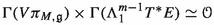. Moreover, following the proof of Theorem 4.2, we also deduce that the Lie brackets in between the previous sections are all zero. Note that if $s_1, s_1$ are sections of the vector bundle $\pi _{M, \mathfrak {g}}: T^*M \otimes \mathfrak {g} \rightarrow M$ then

  $$\begin{aligned}{}[s_1^\textbf{v}, s_2^\textbf{v}] = 0, \; \; i_{s_1^\textbf{v}}d(\pi _{M,\mathfrak {g}}^*\alpha ) = 0, \end{aligned}$$

  for $\alpha \in \Gamma (\Lambda ^{m-1}T^*M)$.

• Consider the linear-affine bracket

  

  for the Hamiltonian field theory which extends Yang–Mills theory. We have that if $\theta = \theta _i(x)dx^{i}$ is a 1-form on M, $\xi = \xi ^\alpha e_\alpha \in \mathfrak {g}$, $\beta = \beta ^{i}(x) d^{m-1}x_i$ is a $(m-1)$-form on M and

  $$\begin{aligned} h(x^{i}, u^\alpha _i, p^{ij}_\alpha ) = (x^{i}, u^\alpha _i, -H(x^{j}, u^\beta _j, p^{jk}_\beta ), p^{ij}_\alpha ) \end{aligned}$$

  is a section of 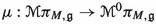then

  $$\begin{aligned} \begin{array}{rcl} \{\widehat{(\theta \otimes \xi )^\textbf{v}}, h \} &{} = &{}\left( \displaystyle \frac{\partial \theta _i}{\partial x^j}(x) \xi ^\alpha p^{ij}_\alpha - \displaystyle \frac{\partial H}{\partial u^\alpha _i}(x^j, u^\beta _j, p^{ij}_\beta )\theta _i(x) \xi ^\alpha \right) d^mx \\ \{\pi _{M, \mathfrak {g}}^*\beta , h\} &{} = &{} \displaystyle \frac{\partial \beta ^i}{\partial x^{i}}d^mx. \end{array} \end{aligned}$$

  In particular, if h is an extension of the Yang–Mills Hamiltonian sectio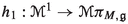n then, is a solution of the Yang–Mills equations if and only if

  

  and

  $$\begin{aligned} \begin{array}{rcl} (s^0)^*(d\widehat{(\theta \otimes \xi )^\textbf{v}}) &{} = &{} \{\widehat{(\theta \otimes \xi )^\textbf{v}}, h \} \circ s^0\\ (s^0)^*(d\beta ) &{} = &{} \{\pi _{M, \mathfrak {g}}^*\beta , h\} \circ s^0, \end{array} \end{aligned}$$

  for $\theta$ a 1-form on M, $\xi \in \mathfrak {g}$ and $\beta$ a $(m-1)$-form on M.

6 Conclusions and future work

In this paper, we have developed a completely canonical geometric formulation of Hamiltonian Classical Field Theories of first order which is analogous to the canonical Poisson formulation of time-independent Hamiltonian Mechanics. This formulation is valid for any configuration bundle and is independent of any external structures such as connections or volume forms. We have defined a space of currents and endowed it with a Lie algebra structure, and we have shown that the bracket induces an affine representation of the Lie algebra of currents on the affine space of Hamiltonian sections. An important difference with the case of time-independent Hamiltonian Mechanics is the linear-affine character of our bracket, which is consistent with the fact that the set of currents and the set of Hamiltonian sections are linear and affine spaces, respectively. We have applied our results to several examples and we have proved their effectiveness.

The results of this paper open some interesting future directions of research:

• Develop appropriate processes of reduction by symmetry for Hamiltonian Classical Field Theories of first order by exploiting the canonical linear-affine bracket formulation proposed in this paper.

• Include boundary conditions in the geometric formulation (see [57]) and discuss the relation between the resultant construction and the theory of Peierls brackets [63] in the space of solutions (see [33, 34]; see also the recent papers [13, 14] and the references therein).

• Discuss a canonical affine formulation of Lagrangian Classical Field Theories of first oder and obtain the equivalence with the Hamiltonian formulation for the case when Lagrangian density is almost regular (this is, for instance, the case of Yang–Mills theories discussed in this paper).

Appendices

The 1-jet bundle associated with a fibration

Let $\pi : E \rightarrow M$ be a fibration, that is, a surjective submersion from E to M. Assume that $dim \; M = m$ and $dim \; E = m+n$.

The 1-jet bundle $J^1\pi$ associated with $\pi$ is the affine bundle over E whose fiber at the point $y \in E$ is

$$\begin{aligned} J_y\pi = \{ z: T_{\pi (y)}M \rightarrow T_yE \mid z \text{ is } \text{ linear } \text{ and } T_y\pi \circ z = id \}. \end{aligned}$$

$J^1\pi$ is modelled over the vector bundle

$$\begin{aligned} V(J^1\pi ) = \pi ^*(T^*M) \otimes V\pi \simeq \cup _{y \in E} \textrm{Lin} (T_{\pi (y)}M, V_y\pi ), \end{aligned}$$

where $V\pi$ is the vertical bundle of $\pi$.

In fact, if $z \in J^1_y\pi$ and $v: T_{\pi (y)}M \rightarrow V_y\pi \in V_y(J^1\pi )$ then one may define, in a natural way, the element $z + v$ of $J^1_y\pi$ as the linear map

$$\begin{aligned} (z + v)(u) = z(u) + v(u), \; \; \text{ for } \text{ all } u \in T_{\pi (y)}M. \end{aligned}$$

If $(x^{i}, u^{\alpha })$ are local coordinates on E which are adapted to the fibration $\pi$ then one may consider the corresponding local coordinates on $J^1\pi$. Indeed, if $z \in J^1_y\pi$, $y \in E$ has local coordinates $(x^{i}, u^{\alpha })$ and

$$\begin{aligned} z\left( \frac{\partial }{\partial x^{i}}_{|\pi (y)}\right) = \frac{\partial }{\partial x^{i}}_{|y} + u^{\alpha } _i \frac{\partial }{\partial u^{\alpha }}_{|y}, \; \; \forall i \in \{1, \ldots , m\}, \end{aligned}$$

then z has local coordinates $(x^{i}, u^{\alpha }, u^{\alpha }_i)$.

Sections of the affine bundle $\pi _{1, 0}: J^1\pi \rightarrow E$ may be identified with Ehresmann connections on the fibration $\pi : E \rightarrow M$.

We recall that an Ehresmann connection on $\pi : E \rightarrow M$ is a vector subbundle H over E of TE satisfying

$$\begin{aligned} TE = H \oplus V\pi . \end{aligned}$$

Note that if H is an Ehresmann connection on $\pi : E \rightarrow M$, then one may define the horizontal lift associated with H as a vector bundle morphism

$$\begin{aligned} ^{H}: E \times _M TM \rightarrow H \subseteq TE \end{aligned}$$

In fact, if $(y, u) \in E \times T_{\pi (y)}M$ then $(y, u)^H$ is the unique vector in $H_y$ whose projection over M is u, that is,

$$\begin{aligned} (T_y\pi )((y, u)^H) = u. \end{aligned}$$

It is clear that the horizontal lift induces, in a natural way, a section $s^H$ of the 1-jet bundle $J^1\pi$. The previous correspondence is one-to-one. Indeed, if

$$\begin{aligned} \left( \frac{\partial }{\partial x^{i}}\right) ^H = \frac{\partial }{\partial x^{i}} + H^{\alpha }_i(x, u) \frac{\partial }{\partial u^{\alpha }}, \end{aligned}$$

then

$$\begin{aligned} s^H(x^{i}, u^{\alpha }) = (x^{i}, u^{\alpha }, H^{\alpha }_i(x, u)). \end{aligned}$$

A (local) section $s: U \subseteq M \rightarrow E$ is said to be horizontal with respect to the Ehresmann connection H if

$$\begin{aligned} (T_xs)(u) \in H(s(x)), \; \; \forall x \in U, \; \; \forall u \in T_xM. \end{aligned}$$

So, if

$$\begin{aligned} s(x^{i}) = (x^{i}, u^{\alpha }(x)), \end{aligned}$$

then s is a horizontal section of H if and only if it satisfies the following system of partial differential equations

$$\begin{aligned} \frac{\partial u^{\alpha }}{\partial x^i} = H^{\alpha }_{i}(x, u(x)), \; \; \forall \; i, \alpha . \end{aligned}$$

The Ehresmann connection H is said to be integrable if the distribution H is completely integrable. In such a case, for every point $y \in E$ there exists a unique horizontal (local) section $s: U \subseteq M \rightarrow E$ of H such that $\pi (y) \in U$ and

$$\begin{aligned} s(\pi (y)) = y. \end{aligned}$$

The vertical lift of a section of a vector bundle

In this appendix, we review the definition of the vertical lift of a section of a vector bundle.

Let $\tau : W \rightarrow M$ be a vector bundle and $s: M \rightarrow W$ a smooth section of $\tau : W \rightarrow M$. Then, one may define the vertical lift $s^\textbf{v}$ of s as a vector field on W given by

$$\begin{aligned} s^\textbf{v}(w) = \frac{d}{dt}_{|t=0}(w + t s(x)), \; \; \, \text{ for } w \in W_x \text{ and } x \in M. \end{aligned}$$

It is clear that $s^\textbf{v}$ is vertical with respect to the vector bundle projection $\tau$.

Next, we will obtain a local expression of $s^\textbf{v}$. For this purpose, we consider local coordinates $(x^{i})$ in an open subset O of M and a local basis $\{e_a\}$ of $\Gamma (W)$ in O. Then, we will denote by $(x^{i}, z^{a})$ the corresponding local coordinates on W. Moreover, if

$$\begin{aligned} s(x^{i}) = s^{a}(x^{i})e_a(x^{i}), \; \; \text{ with } s^{a} \in C^{\infty }(O), \end{aligned}$$

then

$$\begin{aligned} s^\textbf{v}(x^{i}, z^{a}) = s^{a}(x^{i})\frac{\partial }{\partial z^{a}}_{|(x, z)}. \end{aligned}$$

A particular case of the previous situation is the following one.

Let $\pi : E \rightarrow M$ be a fibration, with $dim M = m$, and the multimomentum bundle associated with the fibration $\pi : E \rightarrow M$. It is a vector bundle over E (see Sect. 2.1).

Now, if $\Omega \in \Gamma (\Lambda ^mT^*M)$ is a m-form on M then $\pi ^*\Omega$ is a m-form on E. Moreover, $\pi ^*\Omega$ also is a section of the vector bundle . Thus, one may consider the vertical lift $\Omega ^\textbf{v} := (\pi ^*\Omega )^\textbf{v}$ of $\pi ^*\Omega$ as a $\nu$-vertical vector field on . In fact, if $(x^{i}, u^{\alpha }, p, p_\alpha ^{i})$ are canonical coordinates on as in Sect. 2.1, then

$$\begin{aligned} (d^mx)^\textbf{v} = (dx^1 \wedge \cdots \wedge dx^{m})^\textbf{v} = \frac{\partial }{\partial p}. \end{aligned}$$

(B.1)

Diagram

The diagram below illustrates some of the objects used in the paper and their relations. The arrows with label $(\;)^+$ (resp. $(\;) ^*$) indicate that we associate the vector bundle dual to a given affine (resp. vector) bundle. The four dashed arrows pointing down indicate the associated model vector bundle to a given affine bundle. The diagram illustrates the isomorphism $\sharp ^\textrm{aff}$ of affine bundles and three vector bundle isomorphisms naturally associated to it:

• (1) the vector bundle isomorphism $\sharp =-(\sharp ^\textrm{aff})^+$ obtained by taking (minus) the affine dual to $\sharp ^\textrm{aff}$;

• (2) the vector bundle isomorphism $\sharp ^\textrm{lin}$ naturally induced by $\sharp ^\textrm{aff}$ on the associated model vector bundles;

• (3) the vector bundle isomorphism $-(\sharp ^\textrm{lin})^*$ obtained by taking (minus) the dual to $\sharp ^\textrm{lin}$.

Given a Hamiltonian section $h \in \Gamma ( \mu )$, an observable and a section (the space of sections of the vector bundle associated to $\Gamma ( \mu )$), the diagram also illustrates the sections dh, $d \alpha ^0$, , $\mu _0(d \alpha ^0)$ and the corresponding objects obtained by applying sharp operators, namely $\sharp ^\textrm{aff} dh$, $\sharp d \alpha ^0$, , $-( \sharp ^\textrm{lin}) ^* \mu _0(d \alpha ^0)$. These objects enter into the definition of the three structures $\{\cdot ,\cdot \}$, $\{\cdot ,\cdot \}_l$, as

References

Abraham, R., Marsden, J.E.: Foundations of Mechanics, 2nd ed, revised and enlarged. With the assistance of Tudor Ratiu and Richard Cushman. Benjamin/Cummings Publishing Co., Inc., Advanced Book Program, Reading, MA (1978)
Asorey, M., Ibort, A., Spivak, A.: Admissible boundary conditions for Hamiltonian field theories. Int. J. Geom. Methods Mod. Phys. 14(8), 1740006, 17 pp. (2017)
Başar, Y., Weichert, D.: Nonlinear Continuum Mechanics of Solids: Fundamental Mathematical and Physical Concepts. Springer, Berlin (2000)
Barbero G., Fernando, J., Margalef-Bentabol, J., Varo, V., Villaseñor, E.J.S.: Palatini gravity with nonmetricity, torsion, and boundaries in metric and connection variables. Phys. Rev. D 104(4), Paper No. 044046, 6 pp. (2021)
Barbero G., Fernando, J., Margalef-Bentabol, J., Varo, V., Villaseñor, E.J.S.: Covariant phase space for gravity with boundaries: metric versus tetrad formulations. Phys. Rev. D 104(4), Paper No. 044048, 16 pp. (2021)
Barbero G., Fernando, J., Margalef-Bentabol, J., Varo, V., Villaseñor, E.J.S.: On-shell equivalence of general relativity and Holst theories with nonmetricity, torsion, and boundaries. Phys. Rev. D 105(6), Paper No. 064066, 15 pp. (2022)
Binz, E., Sniatycki, J., Fischer, H.: Geometry of Classical Fields. North-Holland Mathematics Studies, 154. Notas de Matemática (Mathematical Notes), 123. North-Holland Publishing Co., Amsterdam (1988)
Bursztyn, H., Cabrera, A., Iglesias, D.: Multisymplectic Geometry and Lie Groupoids. Geometry, Mechanics, and Dynamics, Fields Institute Communication, 73, pp. 57–73. Springer, New York (2015)
Bursztyn, H., Martínez, Alba N., Rubio, R.: On higher Dirac structures. Int. Math. Res. Not. 2019(5), 1503–1542 (2019)
Campos, C.M., Guzmán, E., Marrero, J.C.: Classical field theories of first order and Lagrangian submanifolds of premultisymplectic manifolds. J. Geom. Mech. 4(1), 1–26 (2012)
Cariñena, J.F., Crampin, M., Ibort, A.: On the multisymplectic formalism for first order field theories. Differ. Geom. Appl. 1(4), 345–374 (1991)
Castrillón López, M., Marsden, J.E.: Some remarks on Lagrangian and Poisson reduction for field theories. J. Geom. Phys. 48(1), 52–83 (2003)
Ciaglia, F.M., Di Cosmo, F., Ibort, A., Marmo, G., Schiavone, L., Zampini, A.: The geometry of the solution space of first order Hamiltonian field theories I: from particle dynamics to free electrodynamics. Preprint arXiv:2208.14136 (2022)
Ciaglia, F.M., Di Cosmo, F., Ibort, A., Marmo, G., Schiavone, L., Zampini, A.: The geometry of the solution space of first order Hamiltonian field theories II: non-Abelian gauge theories. Preprint arXiv:2208.14155 (2022)
Ciaglia, F.M., Di Cosmo, F., Ibort, A., Marmo, G., Schiavone, L., Zampini, A.: Symmetries and covariant Poisson brackets on presymplectic manifolds. Symmetry 14(70), 1–28 (2022)
Ciaglia, F.M., Di Cosmo, F., Ibort, A., Marmo, G., Schiavone, L., Zampini, A.: The geometry of the solution space of first order Hamiltonian field theories III: Palatini’s formulation of general relativity. arXiv:2311.15714 (2023)
Crnkovic, C.: Symplectic geometry of the convariant phase space. Class. Quantum Gravity 5(12), 1557 (1988)
Crnkovic, C., Witten, E.: Covariant description of canonical formalism in geometrical theories. In: Hawking, S.W., Israel, W. (eds.) Three Hundred Years of Gravitation, pp. 676–684. Cambridge University Press, Cambridge (1987)
Chinea, D., de León, M., Marrero, J.C.: The constraint algorithm for time-dependent Lagrangians. J. Math. Phys. 35(7), 3410–3447 (1994)
Demoures, F., Gay-Balmaz, F.: Multisymplectic variational integrators for barotropic and incompressible fluid models with constraints. In: Nielsen, F., Barbaresco, F. (eds.) Geometric Science of Information. GSI 2021. Lecture Notes in Computer Science, vol. 12829. Springer, Cham (2021)
Demoures, F., Gay-Balmaz F.: Unified discrete multisymplectic Lagrangian formulation for hyperelastic solids and barotropic fluids. J. Nonlinear Sci. 32(6), Paper No. 94, 42 pp. (2022)
Demoures, F., Gay-Balmaz, F., Ratiu, T.S.: Multisymplectic variational integrator and space/time symplecticity. Anal. Appl. 14(3), 341–391 (2014)
de León, M., Marín-Solano, J., Marrero, J.C.: Ehresmann Connections in Classical Field Theories. Differential Geometry and Its Applications (Granada, 1994), pp. 73–89. An. Fís. Monographs, 2. CIEMAT, Madrid (1995)
de León, M., Marín-Solano, J., Marrero, J.C.: The constraint algorithm in the jet formalism. Differ. Geom. Appl. 6(3), 275–300 (1996)
de León, M., Marín-Solano, J., Marrero, J.C.: A geometrical approach to classical field theories: a constraint algorithm for singular theories. In: New Developments in Differential Geometry (Debrecen, 1994). Mathematics Application, 350, pp. 291–312. Kluwer Academic Publisher, Dordrecht (1996)
de León, M., Martín de Diego, D., Santamaría-Merino, A.: Symmetries in classical field theory. Int. J. Geom. Methods Mod. Phys. 1(5), 651–710 (2004)
de León, M., Rodrigues, P.R.: Methods of Differential Geometry in Analytical Mechanics. North-Holland Mathematics Studies, 158, North-Holland Publishing Co., Amsterdam (1989)
DeWitt, B.S.: Invariant commutators for the quantized gravitational field. Phys. Rev. Lett. 4(6), 317–320 (1960)
DeWitt, B.S.: Dynamical Theory of Groups and Fields. Gordon and Breach, New York (1965)
Echeverría-Enríquez, A., de León, M., Muñoz-Lecanda, M.C., Román-Roy, N.: Extended Hamiltonian systems in multisymplectic field theories. J. Math. Phys. 48(11), 112901, 30 pp. (2007)
Echeverría-Enríquez, A., Muñoz-Lecanda, M.C., Román-Roy, N.: Multivector field formulation of Hamiltonian field theories: equations and symmetries. J. Phys. A 32(48), 8461–8484 (1999)
Echeverría-Enríquez, A., Muñoz-Lecanda, M.C., Román-Roy, N.: Geometry of multisymplectic Hamiltonian first-order field theories. J. Math. Phys. 41(11), 7402–7444 (2000)
Forger, M., Romero, S.V.: Covariant Poisson brackets in geometric field theory. Commun. Math. Phys. 256(2), 375–410 (2005)
Forger, M., Salles, Mário O.: On covariant Poisson brackets in classical field theory. J. Math. Phys. 56(10), 102901, 26 pp. (2015)
García, P.L., Pérez-Rendón, A.: Symplectic approach to the theory of quantized fields. I. Commun. Math. Phys. 13, 24–44 (1969)
García, P.L., Pérez-Rendón, A.: Symplectic approach to the theory of quantized fields. II. Arch. Ration. Mech. Anal. 43, 101–124 (1971)
García, P.L.: The Poincaré-Cartan invariant in the calculus of variations. In: Symposia Mathematica, vol. XIV (Convegno di Geometria Simplettica e Fisica Matematica, INDAM, Rome, 1973), pp. 219–246. Academic Press, London (1974)
Gay-Balmaz, F., Marsden, J.E., Ratiu, T.S.: Reduced variational formulations in free boundary continuum mechanics. J. Nonlinear Sci. 22(2), 553–597 (2012)
Gay-Balmaz, F.: General relativistic Lagrangian continuum theories part I: reduced variational principles and junction conditions for hydrodynamics and elasticity. J. Nonlinear Sci. 34(46), 1–57 (2024)
Goldschmidt, H., Sternberg, S.: The Hamilton–Cartan formalism in the calculus of variations. Ann. Inst. Fourier 23, 203–267 (1973)
Gotay, Mark J.: A Multisymplectic Framework for Classical Field Theory and the Calculus of Variations. I. Covariant Hamiltonian Formalism. North-Holland Delta Series, pp. 203–235. North-Holland Publishing Co., Amsterdam (1991)
Grabowska, K.: A Tulczyjew triple for classical fields. J. Phys. A 45(14), 145207, 35 pp. (2012)
Grabowska, K., Grabowski, J.: Tulczyjew triples: from statics to field theory. J. Geom. Mech. 5(4), 445–472 (2013)
Grabowska, K., Grabowski, J., Urbański, P.: Lie brackets on affine bundles. Ann. Global Anal. Geom. 24(2), 101–130 (2003)
Grabowska, K., Grabowski, J., Urbański, P.: AV-differential geometry: Poisson and Jacobi structures. J. Geom. Phys. 52(4), 398–446 (2004)
Grabowska, K., Grabowski, J., Urbański, P.: Frame-independent mechanics: geometry on affine bundles. Travaux mathématiques. Fasc. XVI, pp. 107–120. Travel Mathematics, vol. 16. Univ. Luxemb., Luxembourg (2005)
Grabowska, K., Grabowski, J., Urbański, P.: AV-differential geometry: Euler–Lagrange equations. J. Geom. Phys. 57(10), 1984–1998 (2007)
Hansoul, S., Lecomte, P.: Affine representations of Lie algebras and geometric interpretation in the case of smooth manifolds. Int. Math. Res. Not. 16, 981–1003 (2005)
Ibort, A., Spivak, A.: Covariant Hamiltonian field theories on manifolds with boundary: Yang–Mills theories. J. Geom. Mech. 9(1), 47–82 (2017)
Ibort, A.: Spivak, A.: On a covariant Hamiltonian description of Palatini’s gravity on manifolds with boundary. Preprint arXiv:1605.03492
Iglesias, D., Marrero, J.C., Padrón, E., Sosa, D.: Lagrangian submanifolds and dynamics on Lie algebroids. Rep. Math. Phys. 57(3), 385–436 (2006)
Kijowski, J.: A finite-dimensional canonical formalism in the classical field theory. Commun. Math. Phys. 30(2), 99–128 (1973)
Kijowski, J., Szczyrba, W.: A canonical structure for classical field theories. Commun. Math. Phys. 46(2), 183–206 (1976)
Kijowski, J., Tulczyjew, W.M.: A Symplectic Framework for Field Theories. Lecture Notes in Physics, vol. 107. Springer, Berlin (1979)
Lew, A., Marsden, J.E., Ortiz, M., West, M.: Asynchronous variational integrators. Arch. Ration. Mech. Anal. 167(2), 85–146 (2003)
Libermann, P., Marle, C.-M.: Symplectic Geometry and Analytical Mechanics. Translated from the French by Bertram Eugene Schwarzbach. Mathematics and its Applications, 35. D. Reidel Publishing Co., Dordrecht (1987)
Margalef-Bentabol, J., Villaseñor, E.J.S.: Geometric formulation of the covariant phase space methods with boundaries. Phys. Rev. D 103(2), Paper No. 025011, 37 pp. (2021)
Marsden, J.E., Patrick, G.W., Shkoller, S.: Multisymplectic geometry, variational integrators and nonlinear PDEs. Commun. Math. Phys. 199, 351–395 (1998)
Marsden, J.E., Shkoller, S.: Multisymplectic geometry, covariant Hamiltonians, and water waves. Math. Proc. Camb. Philos. Soc. 125(3), 553–575 (1999)
Martínez, E., Mestdag, T., Sarlet, W.: Lie algebroid structures and Lagrangian systems on affine bundles. J. Geom. Phys. 44(1), 70–95 (2002)
Marsden, J.E., Hughes, T.J.R.: Mathematical Foundations of Elasticity. Prentice Hall, New York (1983) (reprinted by Dover, New York, 1994)
Marsden, J.E., Ratiu, T.S.: Introduction to Mechanics and Symmetry. A Basic Exposition of Classical Mechanical Systems. Texts in Applied Mathematics, 17. Springer, New York (1994)
Peierls, R.E.: The commutation laws of relativistic field theory. Proc. R. Soc. Lond. Ser. A 214, 143–157 (1952)
Simo, J.C., Taylor, R.L., Pister, K.S.: Variational and projection methods for the volume constraint in finite deformation elasto-plasticity. Comput. Methods Appl. Mech. Eng. 51, 177–208 (1985)
Volterra, V.: Sulle equazioni differenziali che provengono da questiono di calcolo delle variazioni. Rend. Cont. Acad. Lincei Ser. IV VI, 42–54 (1890)
Volterra, V.: Sopra una estensione della teoria Jacobi-Hamilton del calcolo delle varizioni. Rend. Cont. Acad. Lincei Ser. IV VI, 127–138 (1890)
Funding
Open Access funding provided thanks to the CRUE-CSIC agreement with Springer Nature.
Author information
Authors and Affiliations
Corresponding author
Additional information
Publisher's Note
Springer Nature remains neutral with regard to jurisdictional claims in published maps and institutional affiliations.
J.C.M. and N.M. thank H. Bursztyn, A. Cabrera, S. Capriotti and D. Iglesias for stimulating discussions on the topics of this paper. J.C.M. has been partially supported by the Spanish Ministry of Science and Innovation under grant PID2022-137909NB- C22 and RED2022-134301-T (MCIN/AEI /10.13039/501100011033).