
Abstract
We analyze two algorithms for computing the symplectic factorization A = LLT of a given symmetric positive definite symplectic matrix A. The first algorithm W1 is an implementation of the HHT factorization from Dopico and Johnson (SIAM J. Matrix Anal. Appl. 31(2):650–673, 2009), see Theorem 5.2. The second one is a new algorithm W2 that uses both Cholesky and Reverse Cholesky decompositions of symmetric positive definite matrices. We present a comparison of these algorithms and illustrate their properties by numerical experiments in MATLAB. A particular emphasis is given on symplecticity properties of the computed matrices in floating-point arithmetic.
1 Introduction
We study numerical properties of two algorithms for computing symplectic LLT factorization of a given symmetric positive definite symplectic matrix \(A \in \mathbb {R}^{2n \times 2n}\). A symplectic factorization is the factorization A = LLT, where \(L \in \mathbb {R}^{2n \times 2n}\) is block lower triangular and is symplectic.
Let
where In denotes the n × n identity matrix.
We will write J and I instead of Jn and In when the sizes are clear from the context.
Definition 1
A matrix \(A \in \mathbb {R}^{2n \times 2n}\) is symplectic if and only if ATJA = J.
We can use the symplectic LLT factorization to compute the symplectic QR factorization and the Iwasawa decomposition of a given symplectic matrix via Cholesky decomposition. We can modify Tam’s method, see [1, 7]. Symplectic matrices arise in several applications, among which symplectic formulation of classical mechanics and quantum mechanic, quantum optics, various aspects of mathematical physics, including the application of symplectic block matrices to special relativity, optimal control theory. For more details we refer the reader to [1, 3], and [8].
Partition \(A \in \mathbb {R}^{2n \times 2n}\) conformally with Jn defined by (1) as
in which \(A_{ij} \in \mathbb {R}^{n \times n}\) for i,j = 1,2.
An immediate consequence of Definition 1 is that the matrix A, partitioned as in (2), is symplectic if and only if \(A_{11}^{T} A_{21}\) and \(A_{12}^{T} A_{22}\) are symmetric and \(A_{11}^{T} A_{22}-A_{21}^{T} A_{12}=I\).
Symplectic matrices form a Lie group under matrix multiplications. The product A1A2 of two symplectic matrices \(A_{1}, A_{2} \in \mathbb {R}^{2n \times 2n}\) is also a symplectic matrix. The symplectic group is closed under transposition. If A is symplectic then the inverse of A equals A− 1 = JTATJ, and A− 1 is also symplectic.
Lemmas 1–5 will be helpful in the construction and for testing of some herein proposed algorithms.
Lemma 1
A nonsingular block lower triangular matrix \(L\in \mathbb {R}^{2n \times 2n}\), partitioned as
is symplectic if and only if \(L_{22}=L_{11}^{-T}\) and \(L_{21}^{T} L_{11}=L_{11}^{T} L_{21}\).
Lemma 2
A matrix \(Q \in \mathbb {R}^{2n \times 2n}\) is orthogonal symplectic (i.e., Q is both symplectic and orthogonal) if and only if Q has a form
where \(C, S \in \mathbb {R}^{n \times n}\) and U = C + iS is unitary.
Next, we use the following result from [9], Theorem 2.
Lemma 3
Every symmetric positive definite symplectic matrix \(A \in \mathbb {R}^{2n \times 2n}\) has a spectral decomposition A = Q diag(D,D− 1)QT, where \(Q \in \mathbb {R}^{2n \times 2n}\) is orthogonal symplectic, and D = diag(di), with d1 ≥ d2 ≥… ≥ dn ≥ 1.
In order to create examples of symmetric positive definite symplectic matrices we can use the following result from [3], Theorem 5.2.
Lemma 4
Every symmetric positive definite symplectic matrix \(A \in \mathbb {R}^{2n \times 2n}\) can be written as
where G is symmetric positive definite and C is symmetric.
Lemma 5
Let \(A \in \mathbb {R}^{2n \times 2n}\) be a symmetric positive definite symplectic matrix, partitioned as in (2). Let S be the Schur complement of A11 in A:
Then S is symmetric positive definite and we have
Proof
The property (7) was proved in a more general setting in [3], see Corollary 2.3. We propose an alternative proof for completeness.
It is well known that if A is a symmetric positive definite matrix then the Schur complement S is also symmetric positive definite. We only need to prove (7). Let A be a symmetric positive definite matrix. Then A is symplectic if and only if AJA = J, which is equivalent to the three following conditions:
From (8) we get \(A_{22}=A_{11}^{-1}+ \left (A_{11}^{-1} A_{12}\right ) A_{12}\). We can rewrite (9) as \(A_{12}^{T} A_{11}^{-1}=A_{11}^{-1} A_{12}\). Thus, we have \(A_{22}=A_{11}^{-1}+ A_{12}^{T}A_{11}^{-1}A_{12}\), which together with (6) leads to (7). □
We propose methods for computing symplectic LLT factorization of a given symmetric positive definite symplectic matrix A, where L is symplectic and partitioned as in (3). We apply the Cholesky and the Reverse Cholesky decompositions. Practical algorithm for the Reverse Cholesky decomposition is described in Section 2, see Remark 1.
Theorem 6
Let \(M \in \mathbb {R}^{m \times m}\) be a symmetric positive definite matrix.
- (i):
-
Then there exists a unique lower triangular matrix \(L \in \mathbb {R}^{m \times m}\) with positive diagonal entries such that M = LLT (Cholesky decomposition).
- (ii):
-
Then there exists a unique upper triangular matrix \(U \in \mathbb {R}^{m \times m}\) with positive diagonal entries such that M = UUT (Reverse Cholesky decomposition).
Proof
We only need to prove (ii). Using the fact (i) for the inverse of M, we get \(M^{-1}=\hat {L} \hat {L}^{T}\), where \(\hat {L}\) is a lower triangular matrix with positive diagonal entries. Then \(M=(\hat {L} \hat {L}^{T})^{-1}=U U^{T}\) where \(U=\hat {L}^{-T}\). Clearly, U is upper triangular with positive entries, and U is unique. □
Based on Theorem 6, we prove the following result on symplectic LLT factorization (see [3], Theorem 5.2).
Theorem 7
Let \(A \in \mathbb {R}^{2n \times 2n}\) be a symmetric positive definite symplectic matrix of the form
If \(A_{11}=L_{11} L_{11}^{T}\) is the Cholesky decomposition of A11, then A = LLT, in which
is symplectic.
If S is the Schur complement of A11 in A, defined in (6), and S = UUT is the Reverse Cholesky decomposition of S, then \(L_{22}= L_{11}^{-T} = U\).
Proof
We can write
This gives the identities
Clearly, \(L_{21}^{T}=L_{11}^{-1} A_{12}\), and \(S=A_{22}-L_{21} L_{21}^{T}\) is the Schur complement of A11 in A. Moreover, \(S=L_{22} L_{22}^{T}\). If S = UUT is the Reverse Cholesky decomposition of S and L22 is upper triangular, then L22 = U, by Theorem 6. From Lemma 5 we have \(S=A_{11}^{-1}\), hence \(S= L_{11}^{-T} L_{11}^{-1}\). Notice that \(L_{11}^{-T}\) is upper triangular, so \(U=L_{11}^{-T}\).
It is easy to prove that L in (12) is symplectic. It follows from Lemma 1 and (9). □
The paper is organized as follows. Section 2 describes Algorithms W1 and W2. Section 3 presents both theoretical and practical computational issues. Section 4 is devoted to numerical experiments and comparisons of the methods. Conclusions are given in Section 5.
2 Algorithms
We apply Theorem 7 to develop two algorithms for finding the symplectic LLT factorization. They differ only in a way of computing the matrix L22. Algorithm W1 is based on Theorem 5.2 from [3]. We propose Algorithm W2, which can be used for symmetric positive definite matrix A, not necessarily symplectic. However, if A is additionally symplectic then the factor L is also symplectic.
-
Algorithm W1
Given a symmetric positive definite symplectic matrix \(A \in \mathbb {R}^{2n \times 2n}\). This algorithm computes the symplectic LLT factorization A = LLT, where L is symplectic and has a form
$$ L=\left( \begin{array}{cc} L_{11} & 0 \\ L_{21} & L_{22} \end{array} \right). $$-
Find the Cholesky decomposition \(A_{11}=L_{11}L_{11}^{T}\).
-
Solve the multiple lower triangular system \(L_{11} L_{21}^{T}=A_{12}\) by forward substitution.
-
Solve the lower triangular system L11X = I by forward substitution, i.e., computing each column of \(X=L_{11}^{-1}\) independently, using forward substitution.
-
Take L22 = XT.
Cost: \(\frac {5}{3} n^{3}\) flops.
-
-
Algorithm W2
Given a symmetric positive definite symplectic matrix \(A \in \mathbb {R}^{2n \times 2n}\). This algorithm computes the symplectic LLT factorization A = LLT, where L is symplectic and has a form
$$ L=\left( \begin{array}{cc} L_{11} & 0 \\ L_{21} & L_{22} \end{array} \right). $$-
Find the Cholesky factorization \(A_{11}=L_{11}L_{11}^{T}\).
-
Solve the multiple lower triangular system \(L_{11} L_{21}^{T}=A_{12}\) by forward substitution.
-
Compute the Schur complement \(S=A_{22}- L_{21} L_{21}^{T}\).
-
Find the Reverse Cholesky decomposition \(S=L_{22} L_{22}^{T}\), where L22 is upper triangular matrix with positive diagonal entries.
-
Cost: \(\frac {8}{3} n^{3}\) flops.
Remark 1
The Reverse Cholesky decomposition M = UUT of a symmetric positive definite matrix \(M \in \mathbb {R}^{m \times m}\) can be treated as the Cholesky decomposition of the matrix Mnew = PTMP, where P is the permutation matrix comprising the identity matrix with its column in reverse order. If Mnew = LLT, where L is lower triangular (with positive diagonal entries), then M = UUT, with U = PLPT being upper triangular (with positive diagonal entries).
For example, for m = 3 we have
and
We use the following MATLAB code:

3 Theoretical and practical computational issues
In this work, for any matrix \(X \in \mathbb {R}^{m \times m}\), ∥X∥2 denotes the 2-norm (the spectral norm) of A, and κ2(X) = ∥X− 1∥2 ⋅∥X∥2 is the condition number of a nonsingular matrix X.
This section mainly addresses the problem of measuring the departure of a given matrix from symplecticity. We also touch a few aspects of numerical stability of Algorithms W1 and W2. However, this topic exceeds the scope of this paper.
First we introduce the loss of symplecticity (absolute error) of \(X \in \mathbb {R}^{2n \times 2n}\) as
Clearly, Δ(X) = 0 if and only if X is symplectic. If \(X \in \mathbb {R}^{2n \times 2n}\) is symplectic then X− 1 = JTXTJ, and the condition number of X equals \(\kappa _{2}(X)=\Vert {X}\Vert _{2}^{2}\). However, in practice Δ(X) hardly ever equals 0.
Lemma 8
Let \(X \in \mathbb {R}^{2n \times 2n}\) satisfy Δ(X) < 1. Then X is nonsingular and we have
Proof
Assume that Δ(X) < 1. We first prove that \(\det X \neq 0\).
Define F = XTJX − J. Since JT = −J and J2 = −I2n, we have the identity
Since J is orthogonal, we get ∥JF∥2 = ∥F∥2 = Δ(X) < 1, hence the matrix I2n − JF is nonsingular. Then (15) and the property \(\det J=1\) leads to \((\det X)^{2}=\det (X^{T}JX)=\det (I_{2n}-JF) \neq 0\). Therefore, \(\det X \neq 0\).
To estimate κ2(X), we rewrite (15) as
Taking norms we obtain
This together with ∥JF∥2 = Δ(X) establishes the formula (14). The proof is complete. □
Now we show that the assumption Δ(X) < 1 of Lemma 8 is crucial.
Lemma 9
For every t ≥ 1 and every natural number n there exists a singular matrix \(X \in \mathbb {R}^{2n \times 2n}\) such that Δ(X) = t.
Proof
The proof gives a construction of such matrix X.
Define
where \(D=\sqrt {t-1} diag(1,0, \ldots ,0)\). Clearly, \(\det X=\det D \det (-D)=0\).
Then we have
Therefore, Δ(X) = ∥D2 + In∥2 = ∥diag(t,1,…,1)∥2 = t. This completes the proof. □
Lemma 10
Let \(A \in \mathbb {R}^{2n \times 2n}\) be a symplectic matrix. Suppose that the perturbed matrix \(\hat {A}=A+E\) satisfies
Then \(\hat {A} \neq 0\) and
Proof
We begin by proving that \(\Vert {\hat {A}}\Vert _{2}>0\) for 0 < 𝜖 < 1. Note that ∥A + E∥2 ≥∥A∥2 −∥E∥2. This together with (17) leads to
hence \(\hat {A} \neq 0\).
It remains to estimate \({\Delta } (\hat {A})\). For simplicity of notation, we define
Since A is symplectic, we get ATJA − J = 0, hence F = ATJE + ETJA + ETJE. Taking norms we obtain
Applying (17) yields
From (17) we deduce that \(\Vert {\hat {A}}\Vert _{2}=\Vert {A}\Vert _{2} (1+\beta )\), where ∣β∣ ≤ 𝜖. This together with (17) and (20) gives
which completes the proof. □
According to (18) we introduce the loss of symplecticity (relative error) of nonzero matrix \(A \in \mathbb {R}^{2n \times 2n}\) as
Remark 2
Assume that A is symplectic. Then we have ATJA = J, so taking norms we obtain
We see that ∥A∥2 ≥ 1 for every symplectic matrix A. Therefore, under the hypotheses of Lemma 10 and applying (19) we get the inequality
If ∥A∥2 is large and \(\hat {A}\) is close to A, then \(symp {\hat {A}} << {\Delta } (\hat {A})\). This property is highlighted in our numerical experiments in Section 4.
Proposition 11
Let \(\tilde {L} \in \mathbb {R}^{2n \times 2n}\) be the computed factor of the symplectic factorization A = LLT, where \(A \in \mathbb {R}^{2n \times 2n}\) is a symmetric positive definite symplectic matrix.
Define
Partition \(\tilde {L}\) and F conformally with J as
Then \(F_{21}=-{F_{12}}^{T}\), F22 = 0 and
Moreover, the loss of symplecticity \({\Delta } (\tilde {L})\) can be bounded as follows
Proof
It is easy to check that F is a skew-symmetric matrix satisfying (25), with F22 = 0. Notice that \({\Delta } (\tilde {L})= \Vert {F}\Vert _{2}\). It remains to prove (26).
Write F in a form F = F1 + F2, where
It is obvious that ∥F1∥2 = ∥F11∥2 and ∥F2∥2 = ∥F12∥2, so
. By property of 2-norm, it follows that ∥Fij∥2 ≤∥F∥2 for all i,j = 1,2.
This completes the proof. □
Remark 3
If Algorithm W1 runs to completion in floating-point arithmetic, then \(\tilde {L}_{22}={\tilde {L}_{11}}^{-T} + \mathcal {O}(\varepsilon _{M})\), where εM is machine precision. See [5], pp. 263–264, where the detailed error analysis of methods for inverting triangular matrix was given. Notice that ∥F12∥2 defined by (25) depends only on conditioning of A11, the submatrix of A. Since A is symmetric positive definite it follows that κ2(A11) ≤ κ2(A). However, the loss of symplecticity of \(\tilde {L}\) from Algorithm W2 can be much larger than for Algorithm W1, see our examples presented in Section 4.
Notice that F11 defined by (25) remains the same for both Algorithms W1 and W2.
Now we explain what we mean by numerical stability of algorithms for computing LLT factorization.
The precise definition is the following.
Definition 2
An algorithm W for computing the LLT factorization of a given symmetric positive definite matrix \(A \in \mathbb {R}^{2n \times 2n}\) is numerically stable, if the computed matrix \(\tilde {L} \in \mathbb {R}^{2n \times 2n}\), partitioned as in (24), is the exact factor of the LLT factorization of a slightly perturbed matrix A + δA, with ∥δA∥2 ≤ εMc∥A∥2, where c is a small constant depending upon n, and εM is machine precision.
In practice, we can compute the decomposition error
If dec is of order εM then this is the best result we can achieve in floating-point arithmetic. We emphasize that here we apply numerically stable Cholesky decomposition of symmetric positive definite matrix A11 (see Theorem 10.3 in [5], p. 197), and also numerically stable Reverse Cholesky decomposition of the Schur complement S (defined by (6)) applied in Algorithm W2. Notice that Lemma 5 implies that κ2(S) = κ2(A11). For general symmetric positive definite matrix A we have a weaker bound: κ2(S) ≤ κ2(A), see [2].
4 Numerical experiments
In this section we present numerical tests that show the comparison of Algorithms W1 and W2. All tests were performed in MATLAB ver. R2021a, with machine precision εM ≈ 2.2 ⋅ 10− 16.
We report the following statistics:
-
Δ(A) = ∥ATJA − J∥2 (loss of symplecticity (absolute error) of A),
-
\({sympA}= \frac {\Vert {A^{T}JA-J}\Vert _{2}}{\Vert {A}\Vert _{2}^{2}}\) (loss of symplecticity (relative error) of A),
-
\({dec}_{Algorithm}= \frac {\Vert {A-\tilde {L} {\tilde {L}}^{T}}\Vert _{2}}{\Vert {A}\Vert _{2}}\) (decomposition error),
-
\({\Delta L}_{Algorithm}= \Vert {\tilde {L}^{T}J \tilde {L}-J}\Vert _{2}\) (loss of symplecticity (absolute error) of \(\tilde {L}\)),
-
\({sympL}_{Algorithm}= \frac {\Vert {{\tilde {L}}^{T}J\tilde {L}-J}\Vert _{2}}{\Vert {\tilde {L}}\Vert _{2}^{2}}\) (loss of symplecticity (relative error) of \(\tilde {L}\)),
Example 1
In the first experiment we take A = STS, where S is a symplectic matrix, which was also used in [1] and [7]:
The results are contained in Table 1. We see that Algorithm W1 produces unstable result \(\tilde {L}\), opposite to Algorithm W2.
Example 2
For comparison, in the second experiment we use the same matrix S and repeat the calculations for the inverse of A from Example 1. Since κ2(A− 1) = κ2(A), we see that the condition numbers of A is the same in both Examples 1 and 2. However, here A11 is perfectly well-conditioned, opposite to the previous Example 1. The results are contained in Table 2. Now Algorithm W1 produces numerically stable result \(\tilde {L}\), like Algorithm W2. We observe that for large values of ΔA (in the last columns of Tables 1 and 2) the loss of symplecticity of computed \(\tilde {L}\) is significant.
Example 3
Here A(10 × 10) is generated as follows

Random matrices of entries are from the distribution N(0,1). They were generated by MATLAB function “randn”. Before each usage the random number generator was reset to its initial state.
Here we use Lemmas 2–3 to create the following MATLAB functions:
-
function for generating orthogonal symplectic matrix Q(2n × 2n):
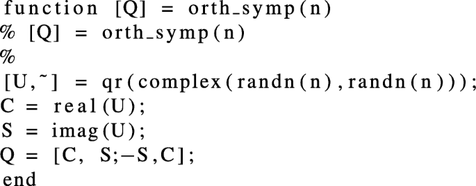
-
and function for generating symmetric positive definite symplectic matrix S(2n × 2n) with prescribed condition number κ2(S) = 102s
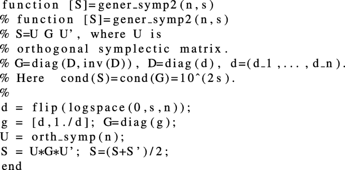


The results are contained in Table 3. However, the results of ∥F12∥2 from Algorithm W2 are catastrophic in comparison with the values received from Algorithm W1. Here A11 is quite well-conditioned, but the departure of A from symplecticity conditions is very large.
Example 4
Now we apply Lemma 4 for creating our test matrices. We take A = PDPT, where
where C is the Hilbert matrix and \({\mathscr{B}}\) is beta matrix.
Here \({\mathscr{B}}=\left (\frac {1}{\beta (i,j)}\right )\), where β(⋅,⋅) is the β function.
By definition,
where Γ(⋅) is the Gamma function.
\({\mathscr{B}}\) is symmetric totally positive matrix of integer. More detailed information related to beta matrix can be found in [4] and [6].
Note that generating A requires computing the inverse of the ill-conditioned Hilbert matrix. It influences significantly on the quality of computed results in floating-point arithmetic.
The results are contained in Table 4.
Example 5
The matrices A(2n × 2n) are generated for n = 2 : 2 : 250 by the following MATLAB code:

We applied Lemma 3 for creating matrices of the form A = UGUT, where G is a diagonal matrix, and U is an orthogonal symplectic matrix, generated by the same MATLAB function as in Example 3.
Figures 1, 2 and 3 illustrate the values of the statistics. We can see the differences between decomposition errors dec (in favor of Algorithm W2) and between the values ΔL, in favor of Algorithm W1.

Condition numbers κ2(A) and decomposition errors for Example 5

The loss of symplecticity (relative errors) for Example 5

The loss of symplecticity (absolute errors) for Example 5
5 Conclusions
-
We analyzed two algorithms W1 and W2 for computing the symplectic LLT factorization of a given symmetric positive definite matrix A(2n × 2n). To assess their practical behavior we performed numerical experiments.
-
Algorithm W1 is cheaper than Algorithm W2. However, Algorithm W1 is unstable for matrices not being exactly symplectic, although it works very well for many test matrices. The decomposition error (27) of the computed matrix \(\tilde {L}\) via Algorithm W1 can be very large. In opposite, in all our tests, Algorithm W2 produces numerically stable resulting matrices \(\tilde {L}\) in floating-point arithmetic (in sense of Definition 2). Numerical stability of Algorithms W1 and W2 remains a topic of future work.
-
Numerical tests presented in Section 4 give indication that the loss of symplecticity of the computed matrix \(\tilde {L}\) from Algorithm W2 can be much larger than obtained from Algorithm W1. We observe that the loss of symplecticity of \(\tilde {L}\) for both Algorithms W1 and W2 strongly depends on the distance from the symplecticity properties (see Lemma 5), and also on conditioning of A and its submatrix A11.
References
Benzi, M., Razouk, N.: On the Iwasawa decomposition of a symplectic matrix. Appl. Math. Lett. 20, 260–265 (2007). https://doi.org/10.1016/j.aml.2006.04.004
Demmel, J.M., Higham, N.J., Schreiber, R.S.: Stability of block LU factorization. Numer. Linear Algebra Appl. 2(2), 173–190 (1995). https://doi.org/10.1002/nla.1680020208
Dopico, F.M., Johnson, C.R.: Parametrization of the matrix symplectic group and applications. SIAM J. Matrix Anal. Appl. 31(2), 650–673 (2009). https://doi.org/10.1137/060678221
Grover, P., Panwar, V.S., Reddy, A.S.: Positivity properties of some special matrices. Linear Algebra Appl. 596, 203–215 (2020). https://doi.org/10.1016/j.laa.2020.03.008
Higham, N.J.: Accuracy and Stability of Numerical Algorithms, 2nd edn. SIAM, Philadelphia (2002)
Higham, N.J., Mikaitis, M.: Anymatrix: an extensible MATLAB matrix collection. Numer. Algoritm. 1–22. https://doi.org/10.1007/s11075-021-01226-2 (2021)
Tam, T.Y.: Computing Iwasawa decomposition of a symplectic matrix by Cholesky factorization. Appl. Math. Lett. 19, 1421–1424 (2006). https://doi.org/10.1016/j.aml.2006.03.001
Lin, W.-W., Mehrmann, V., Xu, H.: Canonical forms for Hamiltonian and symplectic matrices and pencils. Linear Algebra Appl. 302–303, 469–533 (1999). https://doi.org/10.1016/S0024-3795(99)00191-3
Xu, H.: An SVD-like matrix decomposition and its applications. Linear Algebra Appl. 368, 1–24 (2003). https://doi.org/10.1016/S0024-3795(03)00370-7
Author information
Authors and Affiliations
Contributions
The contributions of individual authors to the paper are respectively: dr Maksymilian Bujok, 50%; dr hab. Alicja Smoktunowicz, 30%; dr hab. Grzegorz Borowik, 20%.
Corresponding author
Ethics declarations
Competing interests
The authors declare no competing interests.
Additional information
Publisher’s note
Springer Nature remains neutral with regard to jurisdictional claims in published maps and institutional affiliations.
Rights and permissions
Open Access This article is licensed under a Creative Commons Attribution 4.0 International License, which permits use, sharing, adaptation, distribution and reproduction in any medium or format, as long as you give appropriate credit to the original author(s) and the source, provide a link to the Creative Commons licence, and indicate if changes were made. The images or other third party material in this article are included in the article's Creative Commons licence, unless indicated otherwise in a credit line to the material. If material is not included in the article's Creative Commons licence and your intended use is not permitted by statutory regulation or exceeds the permitted use, you will need to obtain permission directly from the copyright holder. To view a copy of this licence, visit http://creativecommons.org/licenses/by/4.0/.
About this article

Cite this article
Bujok, M., Smoktunowicz, A. & Borowik, G. On computing the symplectic LLT factorization. Numer Algor 93, 1401–1416 (2023). https://doi.org/10.1007/s11075-022-01472-y
Received:
Accepted:
Published:
Issue Date:
DOI: https://doi.org/10.1007/s11075-022-01472-y