
Abstract
Starting from the relationship between Gibbs free energy and equilibrium constant of a chemical reaction (ECCR) and taking into account its temperature dependence according to Kirchhoff, Eq. (12), we arrive at the three-parametric Eq. (26). In going this way, we employ the relationship between the ECCR and the degree of conversion of the solid phase using Eqs. (20) and (21). We find that there is a compensating effect between the coefficients of the equation (i.e., \(a_{1} , a_{2}\)) in the form of a linear equation, which has been attributed to the enthalpy–entropy compensation. According to current state of knowledge, this result applies both to the chemical reactions resulting in individual chemical bond formation as well as in thermal decomposition. When the heat capacity of such chemical reactions decreases linearly along with temperature, it can adopt the value of the (arithmetic mean) average, and the negative sign determines the elements of the functional equations valid for theoretical (Eq. 26) and experimentally fit (Eq. 32) states. For calcite, several possibilities arising from equilibrium changes in the conversion rate vs. temperature are compared by taking into account the CDV L’vov theory.
Introduction
Thermal dissociation is conventionally understood to be a breakdown of chemical bonds in molecules resulting in production of smaller molecules or atoms under the influence of temperature. At this stage we do not consider any quantitative relationship between the substrate and products or their phase transformation. The weaker the chemical bond in a molecule, the lower is the temperature at which thermal dissociation occurs.
For chemical compounds, the following two types of thermal dissociation reactions are typical:
-
(a)
with solid phase and gas phase products being formed
$$({\text{e}} . {\text{g}} .,\,{\text{CaCO}}_{{3 \left( {\text{s}} \right)}} \leftrightarrow {\text{CaO}}_{{\left( {\text{s}} \right)}} + {\text{CO}}_{{2 \left( {\text{g}} \right)}} )$$(1) -
(b)
with only gas phase products being formed from a solid phase substrate
$$({\text{e}} . {\text{g}}.,4{\text{NH}}_{4} {\text{ClO}}_{{4 \left( {\text{s}} \right)}} \to 4{\text{HCl}} + 2{\text{N}}_{2} + 5{\text{O}}_{2} + 6{\text{H}}_{ 2} {\text{O}})$$(2)
Reactions resulting in the thermal dissociation reactions are endothermic. Meanwhile, thermal dissociation occurs reversibly and/or might be irreversible depending on the chemical properties of substances.
Typical reactions involving chemical dissociation processes involving the formation of both solid and gas phases from a single solid phase. In practice the latter algorithm seems to be a definite general rule, although extending this standpoint to all the pyrolysis processes might be problematic because sometimes liquid products appear at ambient temperature as well.
The second basic law of technical and chemical thermodynamics inextricably involves the concept of entropy. According to the postulate by Clausius, the entropy change during an elementary reversible reaction in an isolated system is equal to the ratio between the amount of heat exchange system/its surroundings and the temperature at which this exchange takes place (\({\text{d}}S = \delta Q/T\)). By combining the first and the second basic laws of thermodynamics, Gibbs free enthalpy can be defined as follows:
where all the three terms are functions of the absolute (thermodynamic) temperature T, being taken at some P = const.
For practical purposes, Eq. (3) might very often be replaced by an approximate linear relationship:
In the both above cases, the equilibrium temperature T eq is determined when:
On a numerical scale, the values of \(\Delta H_{\text T}^{o}\) (or A) to \(\Delta S_{\text{T}}^{o}\) (or B) have a ratio of 103:1, but the concept of entropy gives a giant sense of, you might want to quote for Starikov its importance for anthropomorphic nature and agonizing related [1].
Basic CDV L’vov theory
In his 2007 book entitled “Thermal Decomposition of Solids and Melts”, Boris V. L’vov [2] presents a perturbation theory that challenges one to return to classical knowledge.
The relevant work of L’vov began in 1990, while the acronym CDV for his Congruent Dissociative Vaporization (CDV) theory had been introduced in 2007 (see Ref. [6]), and of particular relevance would be his works [3–7]. Meanwhile, since 2007, a number of works has been published in the field, whereas that was Galwey who had methodically analyzed the essence of CDV theory [8, 9] and then published positive reviews on the topic [10, 11]. Remarkably, the Ref. [9] might even be considered an invitation to contribute to the general discussion.
Formally, the process described by the CDV theory can be viewed as a reaction involving the heat of dissociation to yield solid and gas phase products [9]:
or in the short form:
where a, b stand for stoichiometric coefficients acc. L’vov.
Notably, the CDV theory does not consider kinetic models in the classical sense, but assumes that the reactions might proceed in an isothermal and dynamic manner. Thermodynamic considerations can be made for different equilibrium conditions (e.g., equimolar, isobaric, vacuum, etc.), and the conventional concept of reaction rate has been substituted by an overall rate of evaporation J, according to the Hertz–Langmuir equation and using the dimensions (mol m−2 s−1) [7].
According to L’vov, the second basic law of chemical thermodynamics is to be understood as Gibbs free energy (Eq. 3) in conjunction with the balance of chemical reactions by writing [2]:
and it is useful to recast the latter in the following way:
The components of Eq. (9), in accordance with the original symbols [2], have been tabulated and the reaction enthalpy is equal to (assuming the polyisothermal conditions):
which might be re-written by combining A, B and R as:
Let us recall that \(\Delta_{\text{v}} H_{\text{T}}^{\text o}\) indicates the product and applies to the calculation of the gaseous phase. In contrast, \(\tau\) is the coefficient that considers the condensation energy transfer \(\Delta_{\text{c}} H_{\text{T}}^{\text o} \left( A \right)\) of the product A to educt R. This value varies slightly, but it is recommended to accept its value as being equal to \(\tau = {\raise0.7ex\hbox{$1$} \!\mathord{\left/ {\vphantom {1 2}}\right.\kern-0pt} \!\lower0.7ex\hbox{$2$}}\). This is a new element in CDV theory in relation to conventional standpoint. In the similar way, we might calculate the entropy of reaction, as shown in Eq. (10). The value of the constant \(K_{\text{p}}\) is determined experimentally by observing the vapor pressure under the controlled conditions. L’vov has focused most of his work on the experimental studies that confirmed the presence of the solid phase of product A in the gas phase.
Significance of heat capacity for the reaction process
Using Kirchhoff’s laws, the validity of Eq. (9) might be extended to the region of higher temperatures as follows (with omission of the reference symbol to the standard state o where possible):
A novel approach used by Clarke and Glew to solve this problem [12] expresses the dependence of \(\Delta c_{\text{p}}\), on temperature as a Taylor series expansion relative to the temperature difference up to the highest power of \((T - T_{\text{i}} )^{3}\). On the one hand, the advantage of this approach is its capability of expressing thermodynamic functions, including \(\Delta c_{\text{p}}\), at any temperature \(T_{\text{i}}\) (e.g., \(T_{\text{i}} = 298\, {\text{K}}\)). On the other hand, however, the right-hand side of Eq. (12) is comprised of many terms and converges only when \(T < 2T_{\text{i}}\) (see Eq. 7 in [12]).
The Clarke–Glew equation has been used in various works for many other types of processes, for example, research on solubility [13] and phase balances [14, 15].
In our work, we consider that equilibrium occurs during the course of a chemical reaction from the temperature at which the reaction equilibrium constant is infinitely small, but that \(K_{\text{p}} > 0\).
Usually, for thermal dissociation reactions \(\Delta c_{\text{p}} < 0\), the latter can be expressed as a polynomial with sufficient precision:
where the coefficients \(c_{0} , c_{1} , c_{2}\) are tabulated for a wide range of compounds and are hence well known. In substituting specific empirical dependencies, like Eq. (13), into Eq. (12), following integration, gives a large number of components of varying importance in terms of their numerical value.
Analysis of Eq. (12) for thermal dissociation reactions
The full Clarke–Glew equation [12] is rather complex. To maximize its simplification, we assume that the temperature \(T_{\text{i}}\) in Eq. (12) might be chosen in a way to render the relationship in Eq. (13) linear in temperature (i.e., \(c_{2} = 0\)). Bearing this in mind, for the sake of transparency, we accept that the heat capacity of the reaction in the temperature ranges under consideration boils down to the arithmetic average \(\overline{{\Delta c_{\text{p}} }} = C_{\text{p}} = {\text{const}}\). This way we replace the strict form of Eq. (12) with an approximate form embodying all these considerations:
Further, in regard to Eqs. (3), (14) can be converted into the analogous equation reported in Ref. [12], and here we follow this way to demonstrate that all the resulting expressions are dimensionally coherent.
Now Eq. (15) can be analyzed for the case of some thermal decomposition reaction in relation to the product distribution. In following this way, we can first of all introduce the following reversibility identity:
where the term \(K_{\text{p}}^{ - }\) denotes the reverse reaction (backward → forward). Substituting Eq. (16) into Eq. (15) gives, after inversion:
Note the terms in Eqs. (15) and (17), for they will be used in later sections. Additionally, Eqs. (14) and (15) indicate the possibility of internal consistency of their respective terms. Next, we wish to introduce an auxiliary size with the proposed name: heat of the reference state i:
where Eq. (15) now takes the form:
As already mentioned above, the distribution of the simplex (\({\raise0.7ex\hbox{$T$} \!\mathord{\left/ {\vphantom {T {T_{\text{i}} }}}\right.\kern-0pt} \!\lower0.7ex\hbox{${T_{\text{i}} }$}}\)) may lead to some confusion, so it is necessary to place the temperature onto the [K] scale, which stands for a dimensionless logarithmic expression. It is then possible to express the equilibrium constant chemical balance by an equilibrium that gives the degree of transformation as [16–18]:
and
where
In regard to Eqs. (20), (19) mht might be recast as follows:
and, similarly, in regard to Eq. (22):
where
Given that \(\nu = \nu\) or \(\nu = \sum \nu_{\text{i}}\), then Eqs. (23) and (24) give the three-parametric equation:
where the coefficients for the terms ought to be equal to:
Hence, Eq. (27) can be generalized as follows:
Taking into account that the expression \(\Delta H_{\text{i}} + H = \Delta_{\text{R}} H\) defines the average reaction enthalpy, the sense of the parameters \(a_{1} , a_{2}\) becomes clear, while the parameter \(a_{0}\) ought then to determine the sign of \(C_{\text{p}}\).
The importance of the heat of the reference state
Version 1. The elimination of H
It should be noted that the coefficients \(a_{1} , a_{2}\) include the common factor (\({\raise0.7ex\hbox{$H$} \!\mathord{\left/ {\vphantom {H {\nu R}}}\right.\kern-0pt} \!\lower0.7ex\hbox{${\nu R}$}}\)) and are this way inherently interrelated. Clearly, an increase (or decrease) of the value of \(H\) implies an associated increase (or decrease) of the factors listed in Eqs. (27) and (28). Thus, eliminating (\(H\)) requires one to arrive at the functional dependence between the coefficients \(a_{1} , a_{2}\):
For \(a_{2} = 0\), \(a_{1} = {\raise0.7ex\hbox{${\Delta H_{\text{i}} }$} \!\mathord{\left/ {\vphantom {{\Delta H_{\text{i}} } {\nu R}}}\right.\kern-0pt} \!\lower0.7ex\hbox{${\nu R}$}}\), it is necessary to rationalize the change of entropy from the starting temperature \(T_{\text{i}}\). In this sense, we can account for the isokinetic temperature. However, these considerations were with the notion that the temperature has a linear dependence on the temperature for the heat capacity/response process. Under equilibrium conditions Eq. (30) ought to serve as the expression for some compensating effect, which is indeed known in the literature—either as the EEC (enthalpy–entropy compensation) in the literal sense \((\Delta H\, {\text{vs}}.\, \Delta S)\) [1, 19, 20]—or as ‘isolines’ for \(\Delta G_{\text{T}}^{\text o} = {\text{const}}\) according to Eq. (3) [21–23]. Equation (30) in the EEC model corresponds to the concepts of de Marco and Linert [20], as interpreted by Starikov [24], as well as the concept of an iso-equilibrium relationship [25, p. 781]. Meanwhile, according to the work in this field [19–22], the dependency of Eq. (30) might also include an individual chemical compound. Note also that the compatible terms in Eq. (26) for the both coefficients ought to bear the negative and positive signs. Finally, the terms diverge when we perform an inversion procedure, like we have done this for Eqs. (15) and (17).
Version 2. Assumption that \(H = 0\)
In Eq. (24) we assume that \(H = 0\), and according to Eq. (28), immediately arrive at that \(a_{2} = 0\). Equation (26) might then be recast as:
In fact, the resulting expression describes a modified van’t Hoff isobar for the equilibrium temperature, when \({ \ln }\left( {\alpha_{\text{eq}} } \right) = 0,\) then \(T_{\text{eq}} = {\raise0.7ex\hbox{${a_{1} }$} \!\mathord{\left/ {\vphantom {{a_{1} } {a_{0} }}}\right.\kern-0pt} \!\lower0.7ex\hbox{${a_{0} }$}}\).
Further, we bear in mind that the chemical reactions dealing with the thermal dissociation processes ought to be endothermic and accompanied by an increase in the temperature of the surface. Because \(H > 0\), the value of the coefficient in Eq. (29) increases from the starting temperature of \(T_{\text{i}}\), which is contrary to the known observations of these phenomena. However, an analysis of the theory of CDV by L’vov [2–11], we note that the reaction enthalpy for a thermal dissociation process ought to increase with temperature [25]. Thus, the average response intensity for such processes can increase in a classical way. A consequence of this effect is the expression of the EEC effect in Eq. (30).
Experimental dependencies
The three-parametric equation acc. [27] and its linear form for relative reaction rates [28], which were published in 2000–2001, have been used previously [18], and the rules and characteristics of these dependencies have been partially discussed [26] in relation to the analysis of L’vov’s theory, hereafter referred to as CDV. Two of the mentioned equations have the form [27, 28]:
One striking feature of these equations is the compensatory effect of the coefficients \(a_{1}\) on the thermodynamics and \(a_{2}\) on very complex properties, because it applies to both the thermodynamics (Eqs. 27 and 29) and thermokinetics (Eq. 28)—and gives rise to an entropic effect. The linear form of Eq. (34) is similar to Eq. (30):
Meanwhile, the following comment on this thought is now in order.
-
1.
The \(\left( {{\raise0.7ex\hbox{${\Delta_{\text{R}} H}$} \!\mathord{\left/ {\vphantom {{\Delta_{\text{R}} H} \nu }}\right.\kern-0pt} \!\lower0.7ex\hbox{$\nu $}}} \right)\) ratio depends on its interpretation: according to the L’vov theory, a classic \(\nu\) applies only to products, without the participation of the solid phase as the sum of all the stoichiometric coefficients, or to a gas, when the enthalpy of reaction/process is approximately two times greater than the set for each classic \(\nu\).
-
2.
According to this work, Eq. (34) identifies the temperature of the isokinetic sampling \((T_{\text{iso}} )\) under experimental conditions, which does not necessarily create a coordinate that intersects all the data (see Eq. (33) and compare Figs. 4 and 8 in [29]).
-
3.
A formal record of the EEC by [20, 24] (also [25]) is in the form of \(\Delta H = T_{\text{iso}} \Delta S + \Delta H_{\text{iso}}\), and it has the interpretation that it is the enthalpy change of an iso-entropic reaction when \(\Delta S = 0\) [24]. In this context, Eq. (34) presents an attractive form.
As a proper example, we would like to highlight the thermal dissociation of calcite according to [18] and presented in [26] (Fig. 1 in [26]). This example sets the following average enthalpy response to \(a_{2} = 0\). Employing the concept of L’vov, in Eqs. (10) and (11) we use \(\tau = {\raise0.7ex\hbox{$1$} \!\mathord{\left/ {\vphantom {1 2}}\right.\kern-0pt} \!\lower0.7ex\hbox{$2$}}\) and \(\nu = \tau + 1 = 1,5 :465\, {\text{kJ }}\,{\text{mol}}^{ - 1}\) (according to [2, Table 8.2]), 495–544 kJ mol−1 in the temperature range T = 900–1200 K, according to [5] 508.1–498.2 kJ mol−1 in the temperature range T = 900–1200 K (in the CO2 atmosphere); accordingly, 191.4 kJ mol−1 and the value from a classical approach is 174.9 kJ mol−1 [29].
Thus, the average reaction enthalpy/process is strongly dependent on the conditions of the test and the stoichiometric ratio (ν).
This illustration highlights the appropriate dependencies for calcite, which is commonly used as a test case for these purposes. To this end, we used the following equation:
-
(a)
the relationship acc. to Eq. (4), Fig. 1
Fig. 1 
The dependence of the free energy upon the absolute temperature according to Eq. (2), \(\Delta G\) in kJ mol-1
-
(b)
dependence of the degree of equilibrium transformation, \({ \ln }\left( {\alpha_{\text{eq}} } \right)\), vs. the absolute temperature, Fig. 2
Fig. 2 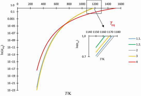
Dependence of \({ \ln }\left( {\alpha_{\text{eq}} } \right) \,{\text{vs}}.\, T\) for different options


Figure 1 depicts our first attempt to make use of the analytical expressions thus obtained to interpret experimental data from all the available sources.
-
1.
∆G = 170.0–0.145T, 800 ≤ T ≤ 1200 K, according to [30], T eq = 1168.6 K
-
2.
∆G = 173.6–0.150T, with Hess’s law (in the environment HCl), according to [31], T eq = 1154.1 K
-
3.
∆G = 141.0–0.130T, from a theoretical decomposition CaC2O4 × H2O, according to [32], T eq = 1084.3 K
-
4.
∆G = 248.0–0.152T, 800 ≤ T ≤ 1200 K, from the data according to [2, Table 16.47], T eq = 1631.6 K
As Fig. 1 shows, if we use the graph 1 as a point of reference, then graph trial 2 deviates insignificantly from our assumptions. The graph 3 is the result of calculations using quantum chemistry and statistical thermodynamics [32] and noticeably lies below the graphs 1 and 2 which have been obtained using relatively more simple approach. The starting point for receipt of calcium carbonate is calcium oxalate, dehydration and decarboxylation, as a result of the emergence of what can be explained by differences of different structures of calcite and consecutive reactions over a wide temperature range: \(298\,{\text{K}}\, \le \,T\, \le \,1273\, {\text{K}}\).
Meanwhile, a complete separation occurs for the graph 4, which results from L’vov’s theory [2] and is presented using the results for the relevant data (Table 16.47 in [2]).
To this end, we used Eq. (3) in the form of thermodynamic functions as suggested by L’vov. According to de Donder, the leveling changes determine how to define the response progress:
Here, in effect, the expression \(\Delta_{\text{r}} H\) could be substituted by Eq. (9) for \(\tau = {1/2}, a = b = 1,\quad {\text{corresponding}}\, {\text{to}}\, \nu = 2\), one obtains the dependence of \(\Delta G \,{\text{vs}}.\, T\), which is nothing more than the linearized form of Eq. (4).
Then, bearing in mind Eq. (2) allows us to characterize the process under study in form of the reaction equilibrium constant’s temperature dependence employing the fundamental equation:
Instead of equilibrium constant in the form of \({ \ln }K_{\text{p}}\), we use either Eq. (18) for the classical theory or Eqs. (21) and (22) according to the L’vov theory. Figure 2 shows these differences in the form of \({ \ln }\left( {\alpha_{\text{eq}} } \right)\,{\text{vs}}.\, T\)
-
1.1.
ln(α eq) = 17.44 − \(\left( {\frac{20447.44}{T}} \right)\), acc. to a straight 1 on Fig. 1
-
1.2.
ln(α eq) = 18.10 − \(\left( {\frac{21039.57}{T}} \right)\), acc. [29]
-
2.
ln(α eq) = 30.633 − \(\left( {\frac{22035.6}{T}} \right)\) − 1.682lnT, acc. [21] for C p = 13.99 J mol−1 K−1
-
3.
ln(α eq) = 26.4 − \(\left( {\frac{22015.0}{T}} \right)\) − 0.983lnT − 0.547*10−3 T + \(\left( {0.343 \times \frac{{10^{5} }}{{T^{2} }}} \right)\), acc. [10, 18] for T i = 400 K and \(\overline{{\Delta c_{\text{p}} }} = - 8.173 - 9.098 \times 10^{ - 3} T + \left( {5.70384 \times \frac{{10^{5} }}{{T^{2} }}} \right)\) when 298 ≤ T ≤ 1200 K,
-
4.
ln(α eq) = 9.834 − \(\left( {\frac{14914.6}{T}} \right)\), acc. to a straight 4 on Fig. 1, and acc. [19] for ν = 2.
As could be seen in Fig. 2, the most accurate dataset refers to the process graphed according to Eq. (5), with some slight deviations for the rest of graphs, except for Eq. (4) resulting from L’vov’s theory. This is why we conclude that the approximation according to the average heat capacity of reaction 2 is acceptable. In accordance with Eq. (26), Fig. 2 shows the correspondence between the signs of the coefficients—namely, where \(a_{1} , a_{2}\) are possessed of negative signs the intercept (\(a_{0}\)) ought to have the positive sign. It should also be noted that under the equilibrium conditions the coefficient \(a_{2}\) has a sufficiently small value, which can be omitted. Indeed, in this case, its value is almost identical to that reported previously [27]. Furthermore, both the Figs. 1 and 2 show the equilibrium temperature (inversion) \(T_{\text{eq}}\) to differ considerably from graph to graph. The relevant data involves curve 4 on Fig. 2 concerning the L’vov theory. It should be stressed that the use of Eq. (3) in the form of Eq. (35) ought to be somewhat speculative. Analysis of the data on the average enthalpy of calcite dissociation cited in Ref. [2] reveals a noticeable effect (increase in almost twice the initial value), and the details in the form of different balances are discussed in the Ref. [26]. However, in comparison with the classical theory, we have used the concept of sharing values of thermodynamic functions for the generated products. Our considerations suggest that the mechanism of CDV becomes more pronounced for very large heating rates. In contrast, the experimentally determined coefficients of the three-parametric Eq. (31), or in the form of Eq. (32) suggest that the enthalpy of reaction is correspondent to the classical data tables (see, for example, [30])—in particular for large values of \(a_{2}\). According to Šesták’s information [33], L’vov theory does not seem to be sufficiently widespread. So that, Eq. (35) ought to be one step forward in developing this theory.
Conclusions
-
1.
Thermal dissociation might be described on the basis of the second basic law of chemical thermodynamics by the Gibbs free enthalpy (Eq. 3) and its relationship to the degree of transformation of the thermodynamic constant for the solid phase (given by Eqs. 21 and 22) to the three-parametric equation (Eq. 26). A small factor of \(a_{2} \ne 0\) may persist, even under equilibrium conditions. One characteristic feature of this work is underlining the correlation between the coefficient signs for each function, that is, when \(a_{1} , a_{2}\) possessed the negative signs (\(a_{0}\)) adopts the positive sign and vice versa, which may also be present for other processes that are not addressed herein (e.g., the suggestion in [27] also according to Ref. [13] in Table 2 for acetonitrile).
-
2.
The relationships of the signs referred to in the above point ought to be a consequence of using Eq. (12) to establish the constancy of the average heat capacity for the process in question, that is, \(C_{\text{p}} = {\text{const}}\) in fact, for the thermal dissociation processes/reactions (and many others), \(C_{\text{p}} < 0\).
-
3.
Experimentally, e.g., using thermogravimetry, a compensatory effect even for individual chemical compounds is described by Eq. (35), with the theoretical basis delivered via Eqs. (27)–(29). This effect includes the EES (enthalpy–entropy compensation) reflecting the mechanistic basis of the process under study. Here, it is noteworthy to recall the interpretation by Starikov: “that entropy’s anthropomorphicity in no way precludes us from inventing some probably seminal interpretational opportunities” [1]. Indeed, it appears that the coefficient \(a_{2}\) arising from entropy changes increases/decreases along with increases/reductions of the reaction/process enthalpy.
-
4.
In accordance with the established L’vov CDV stated in [26], it is possible to use the thermodynamic data for calcite given in [2], Table 16.47, for expressions (Eq. 32), being simpler than the three-parametric equation (Eq. 27). It must be assumed that the form of the expressions suggested by L’vov can be taken to be similar to the thermodynamic changes in the reaction progress according to de Donder. Given the absolute values of the thermodynamic functions, it is possible to consider the effects of thermal dissociation even for infinitely fast heating \(\left( {q \to \infty } \right)\).
Abbreviations
- \(a, b,\nu\) :
-
Stoichiometric coefficients
- \(A, B, R\) :
-
Symbols of chemical compounds
- \(C_{\text p}\; or \;\Delta c_{\text p}\) :
-
Heat capacity, J mol−1 K−1
- \(K\) :
-
Equilibrium constant
- \(P\) :
-
Pressure, Pa
- \(r^{2}\) :
-
Linear coefficient of determination, \(0 \le r^{2} \le 1\)
- \(R\) :
-
Universal gas constant, 8314 J mol−1 K−1
- \(T\) :
-
Temperature, K
- \(q\) :
-
Heating rate, K s−1
- \(\alpha\) :
-
Conversion of the solid phase, \(0 \le \alpha \le 1\)
- \(\delta Q\) :
-
Inexact differential heat
- \(\Delta G, \Delta H, \Delta S\) :
-
Thermodynamic functions, J mol−1
- \(\tau\) :
-
Coefficient considering the condensation energy transfer to reactant acc. L’vov
- \(\varphi\) :
-
Combination of coefficients acc. (22)
- \(o\) :
-
Standard reference condition
- − :
- c :
-
Condensation
- eq :
-
Equilibrium
- f :
-
Formation
- g :
-
Gas
- i :
-
i-th component
- l :
-
Liquid
- p :
-
Pressure activity (fugacity)
- r :
-
Reaction in the L’vov sense
- R :
-
Reaction in the classic sense
- s :
-
Solid
- T :
-
Isothermal conditions
- v :
-
Vaporization
References
Starikov EB. Entropy is anthropomorphic: does this lead to interpretational devalorisation of entropy–enthalpy compensation? Monatsh Chem. 2013;144:97–102.
L’vov BV. Thermal decomposition of solids and melt. Berlin: Springer; 2007.
L’vov BV. Kinetics and mechanism of thermal decomposition of silver oxide. Thermochim Acta. 1999;33:13–9.
L’vov BV. Kinetics and mechanism of thermal decomposition of mercuric oxide. Thermochim Acta. 1999;333:21–6.
L’vov BV, Ugolkov VL. Peculiarities of CaCO3, SrCO3 and BaCO3 decomposition in CO2 as a proof of their primary dissociative evaporation. Thermochim Acta. 2004;410:47–55.
L’vov BV. Dehydration of solids in different modes as a proof of their primary congruent dissociative vaporization. J Therm Anal Calorim. 2006;84:581–7.
L’vov BV, Ugolkov VL. Application of the Hertz–Langmuir equation to studying the kinetics of dehydration of solid compounds in air. Russ J Appl Chem. 2005;78:379–85.
L’vov BV, Galwey AK. Toward a general theory of heterogeneous reactions: thermochemical approach. J Therm Anal Calorim. 2013;113:561–8.
L’vov BV, Galwey AK. Interpretation of the kinetic compensation effect in heterogeneous reactions: thermochemical approach. Int Rev Phys Chem. 2013;32:515–57.
Galwey AK. Theory of solid-state thermal decomposition reactions scientific stagnation or chemical catastrophe? An alternative approach appraised and advocated. J Therm Anal Calorim. 2012;109:1625–35.
Galwey AK. Solid state reaction kinetics, mechanisms and catalysis: a retrospective rational review. React Kinet Mech Catal. 2015;114:1–29.
Clarke ECW, Glew DN. Evaluation of thermodynamic functions from equilibrium constants. Trans Faraday Soc. 1966;62:539–47.
Liu M, Fu H, Yin D, Zhang Y, Lu C, Cao H, Zhou J. Measurement and correlation of the solubility of enrofloxacin in different solvents from (303.15 to 321.05) K. J Chem Eng Data. 2014;59:2070–4.
Monte MJS, Santos LMNBF, Fulem M, Fonseca JMS, Sousa CAD. New static apparatus and vapor pressure of reference materials: naphthalene, benzoic acid, benzophenone, and ferrocene. J Chem Eng Data. 2006;51:757–66.
Monte MJS, Pinto SP, Ferreira AIMCL, Amaral LMPF, Freitas VLS. Fluorene: an extended experimental thermodynamic study. J Chem Thermodyn. 2012;45:53–8.
Błażejowski J. Thermal properties of amine hydrochlorides. Part I. Thermolysis of primary n-alkylammonium chlorides. Thermochim Acta. 1983;68:233–60.
Janiak T, Błażejowski J. Thermal features thermolysis and thermochemistry of hexachlorostannates of some mononitrogen aromatic bases. Thermochim Acta. 1990;157:137–54.
Mianowski A, Siudyga T. Analysis of relative rate of reaction/process. J Therm Anal Calorim. 2012;109:751–62.
Dutronc T, Terazzi E, Piguet C. Melting temperatures deduced from molar volumes: a consequence of the combination of enthalpy/entropy compensation with linear cohesive free-energy densities. RSC Adv. 2014;4:15740–8.
De Marco D, Linert W. Thermodynamic relationships in complex formation. IX. ΔH–ΔS and free energy relationships in mixed ligand complex formation reactions of Cd (II) in aqueous solution. J Chem Thermodyn. 2002;34:1137–49.
Ryde U. A fundamental view of enthalpy–entropy compensation. Med Chem Commun. 2004;5:1324–36.
Olsson TSG, Williams MA, Pitt WR, Lanbury JE. The thermodynamics of protein–ligand interaction and solvation: insights for ligand design. J Mol Biol. 2008;384:1002–17.
Klebe G. Applying thermodynamic profiling in lead finding and optimization. Nat Rev Drug Discov. 2015;14:95–110.
Starikov EB. “Meyer–Neldel rule”: true history of its development and its intimate connection to classical thermodynamics. J Appl Sol Chem Model. 2014;3:15–31.
International Union of Pure and Applied Chemistry. Compendium of chemical terminology. Gold Book. Version 2.3.3. 2.04.2014. http://goldbook.iupac.org/. Accessed 15 Oct 2015.
Mianowski A, Ściążko M. Kinetics of the thermal dissociation in the context L’vov CDV mechanism. Przemysł Chemiczny. 2015;94:496–500 (in Polish).
Mianowski A. Thermal dissociation in dynamic conditions by modeling thermogravimetric curves using the logarithm conversion degree. J Therm Anal Calorim. 2000;59:747–62.
Mianowski A. Analysis of the thermokinetics under dynamic conditions by relative rate of thermal decomposition. J Therm Anal Cal. 2001;63:765–76.
Mianowski A, Baraniec-Mazurek I, Bigda R. Some remarks on equilibrium state in dynamic condition. J Therm Anal Calorim. 2012;107:1155–65.
Barin I. Thermochemical data of pure substance. Weinheim: VCH; 1997.
Odak B, Kosor T. Quick method for determination of equilibrium temperature. J Therm Anal Calorim. 2012;110:991–6.
Błażejowski J, Zadykowicz B. Computational prediction of the pattern of thermal gravimetry data for the thermal decomposition of calcium oxalate monohydrate. J Therm Anal Calorim. 2013;113:1497–1503.
Šesták J. The quandary aspects of non-isothermal kinetics beyond the ICTAC kinetic committee recommendations. Thermochim Acta. 2015;611:26–35.
Acknowledgements
We would like to express our sincere gratitude to Professor Evgeni B. Starikov for his attentive and critical reading of our final version of manuscript and for his substantive and editorial support.
Author information
Authors and Affiliations
Corresponding author
Rights and permissions
Open Access This article is distributed under the terms of the Creative Commons Attribution 4.0 International License (http://creativecommons.org/licenses/by/4.0/), which permits unrestricted use, distribution, and reproduction in any medium, provided you give appropriate credit to the original author(s) and the source, provide a link to the Creative Commons license, and indicate if changes were made.
About this article

Cite this article
Mianowski, A., Urbańczyk, W. Thermal dissociation in terms of the second law of chemical thermodynamics. J Therm Anal Calorim 126, 863–870 (2016). https://doi.org/10.1007/s10973-016-5569-5
Received:
Accepted:
Published:
Issue Date:
DOI: https://doi.org/10.1007/s10973-016-5569-5