
Abstract
Within the emerging age of lunar exploration, optimizing transfer trajectories is a fundamental measure toward achieving more economical and efficient lunar missions. This study addresses the possibility of reducing the fuel cost of two-impulse Earth–Moon transfers in a four-body model with the Earth, the Moon, and the Sun as primaries. Lawden’s primer vector theory is applied within this framework to derive a set of necessary conditions for a fuel-optimal trajectory. These conditions are used to identify which trajectories from an existing database could benefit from the insertion of an additional intermediate impulse. More than 10,000 three-impulse transfers are computed with a direct numerical optimization method. These solutions contribute to enriching the database of impulsive trajectories, useful to perform trade-off analyses. While the majority of trajectories exhibit only marginal improvements, a significant breakthrough emerges for transfers featuring an initial gravity assist at the Moon. Implementing a corrective maneuver after the lunar encounter yields substantial reductions in fuel costs.
1 Introduction
Following the successes of last century’s programs, lunar missions are experiencing a renewed interest. A variety of motivations drive these missions, ranging from the advancing of scientific and technological progress to the unlocking of economic opportunities from extraterrestrial resources, as well as the exploration of the lunar environment and the wider solar system. Notably, the Artemis program (Creech et al. 2022), the Lunar Gateway (Fuller et al. 2022), and the Commercial Lunar Payload Services (CLPS)Footnote 1 initiative represent key milestones in this new age of lunar exploration. Within this framework, maximizing payload mass for Earth–Moon trajectories is a crucial step toward making lunar exploration more accessible and sustainable.
The problem of transferring a spacecraft from an orbit around the Earth to the Moon represents a main challenge from the origin of space exploration. Of special concern are minimum fuel trajectories: if less propellant can be carried, then more payload weight can be thrust into orbit, or smaller spacecraft, e.g., CubeSats, can be used. Several approaches to design Earth–Moon transfers can be found in the literature, and the propulsion technology significantly influences trajectory design (Biesbroek and Janin 2000; Ozimek and Howell 2010; Parker et al. 2013; Capuzzo-Dolcetta and Giancotti 2013; Yoon and Petukhov 2023).
Focusing on impulsive transfers, the complexity of these ranges from simple Hohmann transfers in a two-body model to weak stability boundary transfers with ballistic capture at the Moon in more complete astrodynamical models (Belbruno and Miller 1993; Hatch et al. 2010). Particularly, an initial flyby at the Moon was proved to be a key feature to obtain an Earth–Moon transfer with a cost approaching the theoretical minimum of 3726 m/s, as estimated by Sweetser (1991). Indeed, the most efficient trajectories found in the literature, with costs below 3800 m/s, leverage the presence of the Moon to accomplish an exterior low-energy transfer (Yamakawa et al. 1992, 1993; Qi and Xu 2017). However, some of the limitations associated with these trajectories include the extended transfer time, which exceeds 80 days, and the restricted launch opportunities, requiring precise geometrical alignment of the Earth, the Moon, and the Sun (Circi and Teofilatto 2001).
Topputo (2013) answered the question on the existence of other solutions, having intermediate features. Particularly, the study focuses on two-impulse Earth–Moon transfers accomplished in a totally ballistic fashion, i.e., neither mid-course maneuvers nor other means of propulsion are considered during the cruise. The author revealed the underlying structure that characterizes the \((\Delta t, \, \Delta v)\) space of solutions in a four-body model with the Earth, the Moon, and the Sun as primaries. The transfers were computed through a direct transcription and multiple shooting strategy, so the local optimality of each solution was proved from a numerical viewpoint and against the same class of transfers.
However, even when a direct method is employed, it is beneficial to verify whether the solution satisfies some analytical necessary conditions; otherwise, it cannot be considered an optimal solution (Conway 2010). One method to derive such conditions is by means of primer vector theory, first formulated by Lawden (1963). In his pioneering work, Lawden developed a collection of first-order necessary conditions for the optimality of both impulsive and continuous-thrust trajectories in a two-body model. These conditions are expressed in terms of a particular vector comprised of the adjoin variables associated with the velocity, named primer vector. Lion and Handelsman (1968) extended the theory to non-optimal trajectories, deriving the conditions for the locations and times where additional impulses would improve the cost of the trajectory. These equations were used by Jezewski and Rozendaal (1968) to develop an algorithm for iteratively adding impulses to the trajectory, including a first-order prediction for the magnitude of the interior impulse that leads to the greatest cost reduction. Primer vector theory was tailored to suit the elliptic restricted three-body model by Hiday (1992), who optimized transfers between libration point orbits.
The main starting point for the present work is the dataset of two-impulse solutions found in Topputo (2013). These transfers are seen through the lens of primer vector theory, which is derived from scratch in a four-body model. Presumably, among the numerous solutions available, some already meet Lawden’s criteria, while others could benefit from further modification. The history of the primer vector associated with each trajectory serves to distinguish between optimal and sub-optimal solutions. In the latter case, ways of improving the non-optimal path are sought. Particularly, primer vector is used to assess how the addition of a midcourse impulse can bring improvements to the class of two-impulse Earth–Moon transfers. The newly computed three-impulse trajectories will enrich the existing database, and an updated global picture of optimal multi-impulse Earth–Moon transfers will be provided. Furthermore, it will be possible to evaluate whether some families of transfer benefit more than others from the addition of a third impulse.
The remainder of the paper is structured as follows. In Sect. 2 the background notions are recalled. Section 3 discusses the methodology to reduce the cost of two-impulse Earth–Moon transfers with an additional midcourse impulse. Section 4 shows the results obtained. To conclude, final considerations and critical evaluation are given in Sect. 5.
2 Background
The features of the planar bicircular restricted four-body model (PBRFBM) are reviewed, two-impulse Earth–Moon transfers are defined, and the fuel-optimal problem is stated.
2.1 The planar bicircular restricted four-body model
In the planar bicircular restricted four-body model, two celestial bodies move under their mutual gravity on co-planar circular orbits, about their common center of mass. The two primaries, \(P_1\) and \(P_2\), rotate counterclockwise with a constant angular velocity. On the same plane, the model also incorporates the periodic perturbation of a third celestial body, \(P_3\), which revolves in a circular orbit around the center of mass of the two primaries. The three celestial bodies are assumed to be point masses and to possess spherically symmetric gravity fields. The last body P moves under the gravity of the other three bodies, and in the same plane. The infinitesimal mass of P does not affect the motions of the other bodies.
In the present case, the PBRFBM is used to study the motion of a spacecraft in the cislunar environment. Particularly, \(P_1\) represents the Earth, \(P_2\) the Moon, \(P_3\) the Sun, and P the spacecraft. Despite the model is not coherent, it catches the insights of the real four-body dynamics (Simó et al. 1995; Yagasaki 2004b). Indeed, the bicircular assumption is well-founded, as the eccentricities of the Earth and Moon orbits are 0.0167 and 0.0549, respectively. Similarly, the planar motion is a valid hypothesis because the Moon orbit inclination on the ecliptic is about 5 deg (Meeus 2010).
The motion of the spacecraft is described in a synodic reference frame. The coordinate system (x, y, z) co-rotates with the two primaries and its origin coincides with the Earth–Moon center of mass. The x-axis is parallel to the line joining the two primaries and is directed from the barycenter to \(P_2\). The z-axis is perpendicular to the orbital plane of the primaries. Finally, the y-axis completes the right-handed trial.
The mass-ratio parameter of the problem is defined as \(\mu = M_2/(M_1 + M_2)\), where \(M_1\) and \(M_2\) are the masses of the Earth and the Moon, respectively. Nondimensional quantities are introduced to normalize the problem. The reference length is the mean distance between the two primaries, the mass unit is the sum of the masses of the two primaries, and the time unit is selected such that the nondimensional angular velocity \(\omega \) of the primaries is unitary (Szebehely 1967). The geometry of the problem is depicted in Fig. 1. According to the nondimensional formulation, the Earth and the Moon occupy two fixed points on the rotating x-axis. The values of the physical quantities used in this study are collected in Table 1, together with the reference units of length, time, mass, and velocity.

Geometry of the PBRFBM in rotating Earth–Moon coordinates, drawing not to scale
2.1.1 Equations of motion
The equations describing the motion of a massless particle in the synodic frame of the PBRFBM are (Simó et al. 1995; Yagasaki 2004b)
where the effective potential of the model is defined as
In Eq. (2) the distances of P from \(P_1\), \(P_2\), and \(P_3\) are: \(d_1 = \sqrt{ \left( x+\mu \right) ^2+y^2 }\), \(d_2 = \sqrt{\left( x+\mu -1\right) ^2+y^2 }\), and \(d_3 = \sqrt{ \left( x-\rho \cos (\omega _S t )\right) ^2+\left( y-\rho \sin (\omega _S t )\right) ^2}\). Let the state vector of P in nondimensional rotating coordinates be
where \(\textbf{r} (t) \) is the SC position vector and \(\textbf{v} (t) \) is its velocity vector. Equation (1) in a first-order form becomes
where the coastal acceleration \(\textbf{g}\) is defined as
The quantity \(\textbf{g}\) embeds both the gravitational acceleration as well as the effects due to the relative motion of the rotating frame with respect to an inertial one. The partial derivatives of \(\Omega \) with respect to x and y are reported in Appendix A.1.
The dynamics is also written with a general and compact notation: \(\dot{\textbf{x}} = \textbf{f} (\textbf{x},t)\). Provided an initial condition of the state \(\textbf{x}_{\text {i}} \equiv (\textbf{r}_{\text {i}}, \textbf{v}_{\text {i}})^\top \) at a time \(t_{\text {i}}\), the flow of the PBRFBM, i.e., the solution of Eq. (4), is indicated by \(\varphi (\textbf{x}_{\text {i}}, t_{\text {i}};t)\).
2.1.2 Variational equations
In the paradigm of the PBRFBM, the second-order form of the variational equations reads
where the symbol \(\delta \) indicates the perturbation with respect to a reference solution. \(\varvec{G_r}\) and \(\varvec{G_v}\) are obtained deriving the gravitational acceleration of the model with respect to the position and the velocity vector, respectively.
The solution to the variational state equations is written in terms of the state transition matrix (STM)
The dynamics of \(\varvec{\Phi }\) is described by the first-order variational equation
together with the initial condition \(\varvec{\Phi }(t_{\text {i}},t_{\text {i}})= \varvec{I}_4\). \(\varvec{O}_2\) and \(\varvec{I}_2\) are the null and the identity matrix of size 2, respectively.
2.2 Two-impulse Earth–Moon transfers
The transfers found by Topputo (2013) are the seeding trajectories of this work and will be referred to as reference trajectories. The two-impulse Earth–Moon transfers are defined as follows, where the altitude of the terminal orbits is chosen consistently with the literature (Sweetser 1991; Belbruno and Miller 1993; Yagasaki 2004a; Parker and Anderson 2014).
-
1.
The spacecraft is initially in a circular parking orbit around the Earth, whose altitude is \(h_{\text {i}}= 167\) km;
-
2.
At the initial time \(t_{\text {i}}\), a first impulse \(\Delta \textbf{v}_{\text {i}}\) parallel to the velocity of the parking orbit, places the spacecraft on the transfer orbit;
-
3.
At the final time \(t_{\text {f}}\), a second impulse \(\Delta \textbf{v}_{\text {f}}\) parallel to the local velocity inserts the spacecraft into a circular lunar orbit, of altitude \(h_{\text {f}} = 100\) km.
Both the terminal orbits and the transfer path lie on the (x, y)-plane of the PBRFBM, so that the problem is planar. Similarly, all the trajectories of this work inherit the same terminal conditions and planar properties. Also, maneuvering in the direction of the local velocity is a requirement consistent with a fuel-optimal problem as it maximizes the variations of spacecraft energy (Pernicka et al. 1995).
The solution database of Topputo (2013) is made of almost 280,000 trajectories computed with a direct optimization method. The transfers with \(\Delta t < 100\) days and \(\Delta v < 4150\) m/s are depicted on the \((\Delta t, \Delta v)\)-plane in Fig. 2. Each point is associated with a locally optimal solution with duration \(\Delta t = t_{\text {f}} -t_{\text {i}}\) and cost \(\Delta v = \left\| \Delta \textbf{v}_{\text {i}} \right\| +\left\| \Delta \textbf{v}_{\text {f}}\right\| \). Figure 2 is named global picture and suggests that the solutions are organized into families, which constitute a well-defined structure. To ease the analysis, the total set of solutions is subdivided into two regions that enclose short and long transfers (“S” and “L” frames in Fig. 2). Short transfers are characterized by a time of flight lower than 50 days and a cost below 4150 m/s. Instead, long transfers have a duration between 50 and 100 days.
Note that solutions with a time of flight of up to 200 days exist in the literature (Oshima et al. 2019), and also Earth–Moon transfers requiring as much as 2 years have been found (Bollt and Meiss 1995). However, in this work, a lunar transfer requiring hundreds of days is not deemed a viable option for real missions. Thus, the maximum transfer duration considered is 100 days. As the minimum cost reduces for increasing transfer time, an upper boundary of 4000 m/s encloses long solutions of practical interest for a real mission.

Two-impulse Earth–Moon transfers from Topputo (2013) shown in the (\(\Delta t\), \(\Delta v\)) plane. The two regions S and L enclose short and long transfer solutions, respectively
2.3 Formulation of the fuel-optimal problem
For a spacecraft in the PBRFBM, two class of variables are identified: the augmented-state variables \(\textbf{z}(t) \in \mathbb {R}^{5}\) and the control variables \(\textbf{u}(t) \in \mathbb {R}^{4}\). The augmented-state vector at the time t is the state vector plus the mass of the spacecraft: \(\textbf{z} (t) \equiv \left( \textbf{x}(t),m(t)\right) ^\top \). The control variables \(\textbf{u}(t)\) are related to the action of the engine: \(\textbf{u} (t) \equiv \left( {{\,\mathrm{\text {T}}\,}}(t), \varvec{\alpha } (t), q(t) \right) ^\top \). In particular, \({{\,\mathrm{\text {T}}\,}}(t)\) is the thrust magnitude produced by the engine and \(\varvec{\alpha } (t)\), also known as thrust pointing vector, is a unitary vector in the direction of the thrust. Lastly, q is a slack variable, whose role will be clarified later.
The dynamics of \(\textbf{z}(t)\) is (Conway 2010)
where \(c = g_0 I_{\text {sp}}\) is the effective exhaust velocity, while \(g_0\) = 9.807 m/s\(^2\) is the standard gravitational acceleration and \(I_{\text {sp}}\) is the specific impulse of the engine. Equation (11) can be written with a generic compact notation as \(\dot{\textbf{z}}(t) = \mathbf {f_z} (\textbf{z}(t), \textbf{u}(t), t)\).
In order to find a fuel-optimal trajectory, the mass of propellant consumed must be minimized. In case of a constant specific impulse engine, the cost function \(J \in \mathbb {R}\) to be minimized is (Longuski et al. 2014)
where \(m_{\text {i}}\) and \(m_{\text {f}}\) are the initial and final mass of the spacecraft. Note how, assuming prescribed initial conditions on the mass, J depends only of the final value of the state variable m.
The finite authority of the engine must be taken into account while searching for the histories of the state and control variables minimizing the cost. First, the thrust of the engine is assumed to be bounded: \(0 \le {{\,\mathrm{\text {T}}\,}}(t) \le {{\,\mathrm{\text {T}}\,}}_{\max }\). The last control variable, known as slack variable, \(q \in \mathbb {R}\) is introduced to transform the inequality constraints into an equality one. As a consequence, \({{\,\mathrm{\text {T}}\,}}(t)\) is required to satisfy the following equation
Moreover, by definition, the thrust direction \(\varvec{\alpha }(t)\) is constrained to have unit magnitude: \(\varvec{\alpha }(t)^\top \varvec{\alpha }(t) = 1 .\) Therefore, the values that can be assumed by the control variables are restricted to a specific region U
Let \(\hat{\mathcal {C}}\) denote the class of piecewise continuous functions. The class of admissible control functions in the time interval between \(t_{\text {i}}\) and \(t_{\text {f}}\) is defined as
As this theory will be applied to Earth–Moon transfers discussed in Sect. 2.2, it is pertinent to maintain the same boundary conditions. Consequently, the fuel-optimal problem is formulated for paths with assigned initial position, velocity, and mass \(\textbf{z}(t_{\text {i}})\), and final position and velocity \(\textbf{x}(t_{\text {f}})\). The fuel-optimal problem of this work is stated as follows:
Problem 1
(Fuel-Optimal Problem)
3 Methodology
This section shows how primer vector theory is used to insert an additional intermediate maneuver into non-optimal two-impulse solutions.
3.1 Primer vector theory
Problem 1 falls under the class of optimal control problems with control equality constraints. A set of analytical necessary conditions for the optimality of a fuel-efficient solution in a four-body is derived in terms of the primer vector. However, due to the extensive nature of the underlying theory, only the essential points of the derivation are outlined here (Appendix B contains a complete mathematical discussion).
-
1.
First, a set of Lagrange multiplier \(\varvec{\lambda } \in \mathbb {R}^5\), or costates, is introduced to treat the state equations and the thrust restrictions as differential constraints. Moreover, the adjoint vector to the velocity is termed primer vector and it is indicated with \(\textbf{p}(t)\) (Lawden 1963).
-
2.
Pontryagin Maximum Principle, from optimal control theory, is employed to derive a set of first-order necessary conditions for optimality (Pontryagin et al. 1962).
-
3.
Following Hiday (1992), Weierstrass necessary conditions are discussed for null-thrust, intermediate-thrust and maximum-thrust arcs.
-
4.
The hypothesis of impulsive thrust is made. Consequently, the cost function is rewritten as the characteristic velocity, i.e., the sum of the magnitude of the velocity changes, (Longuski et al. 2014):
$$\begin{aligned} J = \sum _{k=1}^{n_k} \left\| \Delta \textbf{v}(t_k)\right\| \ , \end{aligned}$$(16)where \(t_k\) is the time of the k-th impulse and \(n_k\) is the number of impulsive maneuvers.
-
5.
Due to the presence of corner points, Weierstrass–Erdmann corner conditions from calculus of variations are used to further ease the optimality conditions (Hiday 1992).
-
6.
Finally, further simplifications arise by specifying the gravitational field of the PBRFBM and by expressing everything in terms of the primer vector.
First-order necessary conditions for a fuel-optimal impulsive transfer in the PBRFBM are:
Proposition 1
(Necessary Conditions for an Impulsive Fuel-Optimal Trajectory in the PBRFBM) Consider Problem 1 in a planar bicircular rotating four-body model. The necessary conditions for an impulsive fuel-optimal trajectory require that:
-
1.
The primer vector is continuous, has a continuous first derivative and satisfies
$$\begin{aligned} \ddot{\textbf{p}} = \varvec{G_r} {\textbf{p}} + \varvec{G_v} \dot{\textbf{p}} \ . \end{aligned}$$(17) -
2.
The magnitude of the primer vector is always less or equal than one, with impulses occurring at those instants when the magnitude of the primer is one
$$\begin{aligned} \left\| \textbf{p}(t)\right\| \le 1 \quad \forall \, t \in [t_{\textrm{i}},t_{\textrm{f}}] \quad \text {and} \quad \left\| \textbf{p}( t_k ) \right\| = 1 \quad \forall \, t_k \in [t_{\textrm{i}},t_{\textrm{f}}] \ . \end{aligned}$$(18) -
3.
At all impulses, the primer is a unit vector aligned in the thrust direction
$$\begin{aligned} \textbf{p}(t_k) = \dfrac{\Delta \textbf{v} (t_k)}{\left\| \Delta \textbf{v} (t_k)\right\| }\quad \forall \, t_k \in [t_{\textrm{i}},t_{\textrm{f}}] \ . \end{aligned}$$(19) -
4.
At all interior impulses (not at the initial or final time)
$$\begin{aligned} {\dot{\textbf{p}}(t_k)}^\top \textbf{p}(t_k)= 0 \quad \forall \, t_k \in (t_{\textrm{i}},t_{\textrm{f}}) \ . \end{aligned}$$(20)
The previous conditions coincide with those derived by Hiday (1992), Bell (1995), and Jezewski (1975) in others astrodynamical models. However, this result could not be assumed a priori, since some mathematical passages are different from the existing literature (see Appendix B). Also, except for the inclusion of the matrix \(\varvec{G_v}\) in the differential primer equation, the necessary conditions in Proposition 1 are identical to those obtained by Lawden (1963) for optimal transfers in a two-body problem. Because of this, henceforward they will be referred to as Lawden’s necessary conditions (LNC), and the term “optimal” will be used as a substitute for “meets the first-order LNC”.
3.2 Non-optimal trajectories
Let \(\overline{\gamma }(\overline{\textbf{x}}_{\text {i}}, t_{\text {i}}) := \varphi (\overline{\textbf{x}}_{\text {i}},t_{\text {i}};t) \ \forall t \in [t_{\text {i}},t_{\text {f}}] \) be a two-impulse reference trajectory, which connects two given states \(\overline{\textbf{x}}_{\text {i}}\) and \(\overline{\textbf{x}}_{\text {f}}\) (in the present work, the overlined variables are related to the reference trajectory). The impulses are provided at the initial and final times: \(\Delta \overline{\textbf{v}}_{\text {i}}\) at \(t=t_{\text {i}}\) and \(\Delta \overline{\textbf{v}}_{\text {f}}\) at \(t=t_{\text {f}}\). The primer \(\overline{\textbf{p}}\) is defined as the solution to Eq. (17) which satisfies the following boundary conditions (from Eq. 19)
If a trajectory does not comply with LNC, ways of improving the non-optimal path are sought. Particularly, an impulsive trajectory can be modified in two ways (Conway 2010). One method involves allowing for a terminal coast (either initial or final), while the other entails incorporating a midcourse impulse. However, the present work focuses on modifying the reference trajectories while keeping the same set of boundary conditions and transfer time. Therefore, the addition of a terminal coast is not addressed hereafter.
Figure 3 shows three cases of primer vector qualitative behavior. The dash-dotted black line corresponds to an optimal two-impulse trajectory, for which additional maneuvers would not yield any benefits. The solid dark-gray line represents a typical scenario for an optimal three-impulse transfer, while the dotted light-gray curve indicates a non-optimal trajectory due to the primer magnitude exceeding unity. The objective of the present analysis is to modify a two-impulse reference solution that exhibits a primer behavior akin to the light-gray curve, and to compute an neighboring three-impulse trajectory with a primer history resembling the dark-gray one. The methodology presented to insert a new midcourse impulse to \(\overline{\gamma }\) is inspired by Hiday (1992), and it parallels Lion and Handelsman (1968) extension of primer vector theory to non-optimal trajectories in the two-body problem.

Three cases of primer vector qualitative behavior for an impulsive transfer. These categories are intended to provide representative examples of primer behavior rather than an exhaustive list
3.3 Insertion of a midcourse impulse
To investigate the effect of an additional impulse, the reference two-impulse trajectory \(\overline{\gamma }\) is compared with a neighboring trajectory \({\gamma }\), named perturbed trajectory, to which an interior impulse is added (see Fig. 4). Let the superscripts ‘+’ and ‘–’ denote the evaluation of the quantity prior to and subsequent to the impulsive maneuver. Both trajectories connect the same terminal states: \(\overline{\textbf{x}}_{{\text {i}}^-} = {\textbf{x}}_{{\text {i}}^-}\) at \(t = t_{{\text {i}}^-}\) and \(\overline{\textbf{x}}_{{\text {f}}^+} = {\textbf{x}}_{{\text {f}}^+}\) at \(t = t_{{\text {f}}^+}\). However, at an intermediate time \(t=t_m\), \(\overline{\gamma }\) and \({\gamma }\) pass thorough two different midpoints: \(\overline{\textbf{x}}_m\) and \(\textbf{x}_m\), respectively. This is possible only assuming dissimilar terminal impulses, so: \(\overline{\textbf{v}}_{{\text {i}}^+} \ne {\textbf{v}}_{{\text {i}}^+}\) and \(\overline{\textbf{v}}_{{\text {f}}^-} \ne {\textbf{v}}_{{\text {f}}^-}\). Note that, as the maneuvers are impulsive, the positions are always continuous and do not necessitate the previous notation (e.g., \(\textbf{r}_{\text {i}} = \textbf{r}_{{\text {i}}^+} = \textbf{r}_{{\text {i}}^-}\)).

Two-impulse reference and three-impulse perturbed transfers (in black and red, respectively); \(\overline{\gamma }\) and \({\gamma }\) share the same terminal conditions and transfer time; the midcourse impulse of the latter is located at time \(t_m\); the two enlargements show the velocity vectors at the initial and final impulses
3.3.1 Cost variation
The cost associated with \(\gamma \) and \(\overline{\gamma }\) is, respectively,
The cost \(J_{{\gamma }}\) can be written in terms of the variations with respect to the reference trajectory
where the symbol \(\delta \) is used to express the difference between the perturbed and the reference trajectory (e.g., \(\delta \Delta \textbf{v}_{m} = \textbf{v}_{m}- \overline{\textbf{v}}_{m}\)). As long as the two trajectories share the same terminal states (before the initial impulse and after the final impulse): \(\delta \Delta \textbf{v}_{\text {i}} = \delta \textbf{v}_{{\text {i}}^+}\) and \(\delta \Delta \textbf{v}_{\text {f}} = -\delta \textbf{v}_{{\text {f}}^-}\). Moreover, the velocity on the reference trajectory is continuous at \(t=t_m\), and so \( \Delta \overline{\textbf{v}}_m = \varvec{0}\). Accordingly, the cost variation \(\delta J = J_{\gamma } - J_{\overline{\gamma }}\) is
The differences between the magnitudes of two vectors can be written, to the first-order, as (Jezewski 1975)
Substituting Eqs. (25a) and (25b) into Eq. (24) and recalling that the primer is a unit vector aligned with the velocity increments (Eq. 21), the cost variation results in
Another important outcome of primer vector theory is known as adjoint equation. The finding is originally obtained by Hiday (1992) within the framework of the elliptic restricted three-body model, but it holds true for the PBRFBM as well. Particularly, it asserts that, on a coastal arc (i.e., no impulses exist interior to the terminal impulses), the variational expression \(\textbf{p}^\top \delta {\textbf{v}} -\left( \dot{\textbf{p}}^\top + {\textbf{p}}^\top \varvec{G_v} \right) \delta \textbf{r}\) is constant. Therefore, it can be evaluated at the boundaries of the two coastal arcs composing \(\gamma \).
On the first arc, which originates at \(\left\{ \textbf{x}_{{\text {i}}^+},t_{{\text {i}}^+}\right\} \) and terminates at \(\left\{ \textbf{x}_{m^-},t_{m^-}\right\} \):
where \(c_1\) is a constant. Recalling that \(\delta \textbf{r}_{{\text {i}}^+} = \varvec{0}\) and equating the two expressions
On the second arc, which originates at \(\left\{ \textbf{x}_{m^+},t_{m^+}\right\} \) and terminates at \(\left\{ \textbf{x}_{{\text {f}}^-},t_{{\text {f}}^-}\right\} \):
where \(c_2\) is another constant. Since \(\delta \textbf{r}_{{\text {f}}^-} = \varvec{0}\), equating the two expressions yields
Subtracting Eq. (30) from Eq. (28)
Since the primer vector and its derivative are evaluated on the reference trajectory \(\overline{\gamma }\), which is a coastal arc, \(\overline{\textbf{p}}_m\) and \(\dot{\overline{\textbf{p}}}_m\) are continuous. Similarly, also \(\overline{\textbf{x}}\) is continuous at \(t=t_m\), and so \(\overline{\varvec{G_v}}_{m}\) is continuous as well. Thus, for these three quantities the ‘+’ and ‘–’ subscripts can be dropped. Moreover, although a discontinuity in the velocity is allowed for \(\gamma \) at \(t = t_m\), the position still requires to be continuous; thus, Eq. (31) becomes
Eq. (32) is replaced into the first-order variation of the cost (Eq. (26)):
Let \(\kappa \) denote the magnitude of the intermediate impulse, and \(\hat{\varvec{\kappa }}\) be the unit vector in the direction of the impulse. Substituting \(\Delta {\textbf{v}}_{m} \equiv \delta {\textbf{v}}_{m^+}- \delta {\textbf{v}}_{m^-}\) with \(\kappa \hat{\varvec{\kappa }}\) into Eq. (33), the final expression of the cost variation results in
Equation (34) expresses \(\delta J\) solely in terms of the primer vector at the interior impulse and the intermediate velocity increment. If \(\delta J\) can be made negative, then \(\gamma \) represents an improvement in the cost over \(\overline{\gamma }\). This is possible only if the magnitude of the primer vector at \(t= t_m\) is greater than unity. Therefore, Eq. (34) can be interpreted as an alternate proof of LNC for \(\overline{\gamma }\) to be optimal. The criterion for the insertion of an intermediate impulse on a trajectory in order to reduce the overall cost is:
Proposition 2
(Criterion for an Additional Midcourse Impulse)
Additionally, Eq. (34) suggests that the greatest improvement in cost, to first-order, occurs when the product \(\overline{\textbf{p}}_{m}^\top \hat{\varvec{\kappa }}\) is maximum. This is obtained by applying the intermediate impulse in the direction of the primer at the instant of maximum primer magnitude. However, the position, as well as the magnitude of the interior impulse, is yet to be determined. The location of the new impulse in space and time is done in two steps. The first step is to determine some initial values for the position and the time midcourse impulse that will lower the cost. The second step is to iterate on the values until a minimum in the cost is achieved.
3.3.2 Perturbed three-impulse trajectory
The time of maximum primer magnitude is selected as an initial estimate for \(t_m\). Regrettably, this choice does not guarantee that \(\delta J\) is minimized, because the value of \(\Delta \textbf{v}_m\) cannot be chosen independently from \(t_m\). However, what is needed is just an initial guess to start an iteration process. So, as long as the initial choice produces a negative \(\delta J\), it is decided for the simple device of choosing \(t_m\) as the time of maximum primer magnitude (Conway 2010). The initial position of the impulse, namely the value \(\delta \textbf{r}_m\) to be added to \(\overline{\textbf{r}}_m\), is chosen so that the velocity change is in the direction of the primer vector, in accordance with LNC. Following the first-order analysis based on the STM presented in Jezewski and Rozendaal (1968) and Lion and Handelsman (1968), the first initial guess is
where the matrix \(\varvec{K}\) must be nonsingular and is defined as
If the value of \(\kappa \) is selected small enough to justify a first-order analysis, the previous choice for \(\delta \textbf{r}_m\) ensures that \(\Delta \textbf{v}_m \) and \(\overline{\textbf{p}}_m\) are aligned at the time \(t_m\) when \(\left\| \overline{\textbf{p}}(t)\right\| \) is maximum, which is compliant with the third LNC.
Once the location in time and space of the midcourse impulse is determined, the perturbed trajectory is computed by connecting the prescribed initial and final states with the newly computed position of the intermediate maneuver. To this purpose, a double shooting problem is set up, which consists in solving two Lambert’s problems:
-
connecting the states \(\left\{ \overline{\textbf{r}}_{\text {i}}, \, t_{\text {i}}\right\} \) with \(\left\{ \overline{\textbf{r}}_m + \delta \textbf{r}_m, \, t_m\right\} \);
-
connecting the states \(\left\{ \overline{\textbf{r}}_{\text {f}}, \, t_{\text {f}}\right\} \) with \(\left\{ \overline{\textbf{r}}_m + \delta \textbf{r}_m, \, t_m\right\} \).
The unknowns of the problem are the initial velocity just after the first impulse \(\textbf{v}_{{\text {i}}^+}\) and the final one before the last maneuver \(\textbf{v}_{{\text {f}}^-}\).
The idea of the solution method, represented in Fig. 5, consists in guessing the values of \(\textbf{v}_{{\text {i}}^+}\) and \(\textbf{v}_{{\text {f}}^-}\) and propagating the two states (forward and backward in time) until the continuity on the position is satisfied. Moreover, the two red arcs of Fig. 5 must meet at a precise position specified by \(\overline{\textbf{r}}_m +\delta \textbf{r}_m\). A root-finding problem with four unknowns and a four-dimensional objective function (recall that the current model is planar, so only two coordinates are of interest) is stated as follows:
Problem 2
(Forward–Backward Shooting)

Representation of the forward–backward shooting problem solved to build the perturbed trajectory (in red), whose midcourse impulse occurs at \(t = {t}_m\) and is located at \( \textbf{r}_m = \overline{\textbf{r}}_m + \delta \textbf{r}_m \)
After determining the values of the unknowns, the perturbed trajectory is completely determined, and its cost can be computed: \(J_{\gamma } = \left\| \textbf{v}_{{\text {i}}^+}- \overline{\textbf{v}}_{{\text {i}}^-}\right\| + \kappa + \left\| \overline{\textbf{v}}_{{\text {f}}^+} - \textbf{v}_{{\text {f}}^-}\right\| \). Problem 2 is solved by means of an iterative procedure. The values for the first guess of the unknowns are computed by adding the first-order variations generated by \(\delta \textbf{r}_{m}\) to the velocities of the reference trajectory:
Moreover, the Jacobian of the objective function \(\textbf{F}\) is computed analytically for higher computational efficiency of the gradient-based algorithm employed. Thanks to the choice of the unknowns, the expressions of the derivatives are:
3.4 Movement of the interior impulse
The inclusion of an additional impulse discussed up to this point does not necessarily yield an optimal three-impulse trajectory. The time history of the primer vector magnitude on the perturbed trajectory must be examined again to verify the compliance with LNC. A typical non-optimal trajectory is characterized by a cusp at the location of the intermediate impulse. Therefore, \(\dot{\textbf{p}}\) is not continuous at the interior impulse, and a neighboring three-impulse solution, named refined trajectory, with a lower cost must exist.
Let \(\widetilde{\gamma }\) denote a refined three-impulse trajectory, which shares the same terminal conditions with \(\overline{\gamma }\) and \({\gamma }\). (The tilde symbol will be employed to address quantities associated with the refined trajectory.) However, differently from the perturbed trajectory, the midcourse impulse is allowed to be located at \(\widetilde{t}_m \ne t_m\). \(\widetilde{\gamma }\) consists of two coastal arcs connecting the states \(\left\{ \overline{\textbf{r}}_{\text {i}}, \, t_{\text {i}}\right\} \rightarrow \left\{ \widetilde{\textbf{r}}_m \, \widetilde{t}_m \right\} \) and \(\left\{ \widetilde{\textbf{r}}_m \, \widetilde{t}_m \right\} \rightarrow \left\{ \overline{\textbf{r}}_{\text {f}}, \, t_{\text {f}}\right\} \). If the symbol \(\widetilde{\delta }\) indicates a non-contemporaneous variation, then the position and time of the intermediate maneuver on the refined trajectory can be expressed as
The expression for the cost difference between the refined and the reference three-impulse trajectory is to the first-order (Jezewski and Rozendaal 1968):
Note that when the refined trajectory is optimal, \(\widetilde{\delta } J = 0\); consequently, both the Hamiltonian \(\mathcal {H} := \varvec{\lambda }^\top \mathbf {f_z}\) and the primer derivative must be continuous across the intermediate impulse (see Appendix B).
3.5 Refined three-impulse trajectory
The idea shown in Fig. 6 is to iterate on the position and time of the mid-course impulse, in the neighborhood of the perturbed trajectory \(\gamma \), until a local minimum of \(J_{\widetilde{\gamma }}\) is reached. This can be done by setting up a nonlinear programming (NLP) problem, whose unknowns are \(\widetilde{\textbf{r}}_m\) and \(\widetilde{t}_m\). However, the two arcs of the solution must meet at the position of the second impulse (i.e., it must be \(\widetilde{\textbf{r}}_{m^-}=\widetilde{\textbf{r}}_{m^+}\) in Fig. 6) and this depends on the velocities just after the initial impulse and before the last one. Therefore, to avoid solving a shooting problem at each iteration of the NLP problem, both \(\widetilde{\textbf{v}}_{{\text {i}}^+}\) and \(\widetilde{\textbf{v}}_{{\text {f}}^-}\) are included among the unknowns of the problem. These are collected in a vector of NLP variables \(\textbf{y} =\left( \widetilde{\textbf{v}}_{{\text {i}}^+}, \, \widetilde{\textbf{v}}_{{\text {f}}^-}, \, \widetilde{\textbf{r}}_m,\, \widetilde{t}_m\right) ^\top \in \mathbb {R}^7\).

Optimization problem solved to compute the three-impulse refined trajectory (blue), starting from a three-impulse perturbed trajectory (red)
In such a way, the continuity on the position at \(\widetilde{t}_{m}\) is treated as a nonlinear equality constraint. Also, the time of the midcourse impulse must be within the interval delimited by \(t_{\text {i}}\) and \(t_{\text {f}}\). In the end, the problem is converted into a parameter optimization problem, with a scalar objective function, four scalar equality constraints and two inequality constraints.
Problem 3
(Three-Impulse Trajectory Optimization)
subject to the constraints
Problem 3 is solved numerically with an iterative approach. The components of the first guess solution \({\textbf{y}}^{(0)}\) are taken from the perturbed three-impulse trajectory \(\gamma \): \( {\textbf{y}}^{(0)} = \left( \textbf{v}_{m^+}, \, \textbf{v}_{{\text {f}}^-}, \, \textbf{r}_m,\, {t}_m \right) ^\top .\) Again, the derivatives of \(J_{\widetilde{\gamma }}\) and \(\textbf{h}_{m^-}\), \(\textbf{h}_{m^+}\) with respect to \(\textbf{y}\) are computed analytically for numerical efficiency, and they are reported in Appendix A.2.
4 Results
The methodology presented is now applied to identify the non-optimal solutions of the global picture and to insert an additional intermediate impulse.
The equations of motion of the PBRFBM do not possess an analytical solution; therefore, Eqs. (4) and (10) are integrated numerically, and a variable-step, variable-order Adams–Bashforth–Moulton solver of orders 1 to 13 is used. Both absolute and relative error tolerances are set to \(10^{-12}\). Recalling that all variables are nondimensional, this corresponds to a tolerance lower than 1 mm on the position and \(10^{-6}\) mm/s on the velocity.
4.1 Non-optimal two-impulse Earth–Moon transfers
The primer magnitude associated with each of the reference trajectories is analyzed to verify the optimality of the solutions according to the LNC. However, since the total number of solutions found by Topputo (2013) is 284,013, it is decided to focus only on the transfers inside the S and L regions, due to their more interesting characteristics from the viewpoint of a real lunar mission. Then, the solutions whose primer magnitude exceeds unity are spotted and reported in Fig. 7, where all the colored (gray, red, and blue) points correspond to the non-optimal short and long transfers.
Actually, not all these trajectories are further improved with a midcourse impulse. The gray points in Fig. 7 are still not of practical interest for a real-life mission to the Moon. For instance, long transfers that perform many flybys at the Earth are rarely implemented, as the recursive passage inside the Van Allen belts must be avoided to preserve the hardware of the spacecraft. Moreover, it is observed that the maximum primer magnitude of these trajectories occurs in the vicinity of the Earth. Here the effective potential of the PBRFBM shows very high gradients (Dei Tos and Topputo 2017), and thus, a first-order analysis based on the STM loses accuracy. (This has also repercussions on numerical computations making the integration scheme diverging.) Hence, non-optimal transfers are further filtered and only solutions respecting the following requirements are retained:
-
1.
the trajectory must pass at a distance lower than 40,000 km from the Earth (estimated extension of the outer Van Allen belt) only once, at the departure;
-
2.
during long transfers the spacecraft must not perform more than 2 revolutions about the Earth, while for short transfers the threshold is lowered to 1.5 revolutions.
Red and blue dots reported in Fig. 7 are the retained solutions to which a further impulse is added, while the gray dots are the non-optimal solution discarded by the filter.
-
The solutions contained in the S region are 166,813. Almost 35% of them do not respect LNC, but only 1.5% (2355 solutions) are retained after the filtering. This happens because, in the center of this area, many transfers (belonging to families b and c in Topputo 2013) perform Earth flybys, and so are discarded (note the high number of gray dots at the middle of the red rectangle in Fig. 7). Moreover, note that none of the direct transfers in Fig. 7 (solutions with \(\Delta t < 10 \) day, family a) requires an additional impulse, as they are already optimal.
-
The solutions within the L region are 76,392, and 13% of them do not respect LNC. In this case, many of these last pass the filter (8218 solutions), corresponding to 10.7% of the total number inside the region. However, the majority of the Pareto front solutions, with \(\Delta v < 3850\) m/s and \( \Delta t > 70 \) days, made of low-energy transfers with ballistic capture, do not require a third maneuver. On the contrary, the bigger cluster of improvable solutions is shifted to the top-left corner of the L region. Additionally, there are two vertical blue arcs on the left side of the L region, made of solutions which perform an initial lunar gravity assist. Figure 8 shows the geometry of a non-optimal sample solution of this kind, with \(\Delta v = 3925.3\) m/s and \(\Delta t = 53.5\) days.

Short and long transfers from the global picture. Black dots represent solutions that already satisfy LNC; red and blue points denote non-optimal trajectories belonging to the S and L region that are improved with a midcourse impulse; gray dots indicate non-optimal transfers that are filtered out due to their geometry

Geometry of a sample reference transfer (\(\Delta v = 3925.3\) m/s, \(\Delta t = 53.5\) days) in both synodic (top-left) and Earth-sidereal (top-right) frame, together with the primer magnitude history (bottom graph); Moon’s orbit is depicted with a dashed-gray line in the sidereal frame; the apparent orbit of the Sun (not to scale) is represented in orange; the initial and final position of the Sun is indicated by a filled and an empty circle, respectively; the red cross denotes the instant when the primer magnitude is maximum, and the orange cross specifies the position of the Sun at that time
4.2 Perturbed three-impulse transfers
Once a non-optimal reference transfer is individuated, a perturbed three-impulse trajectory is built by adding a midcourse impulse. The only parameter that is still to be chosen is the magnitude of the midcourse impulse \(\kappa \). Indeed, once this is fixed, the position of the midcourse impulse is obtained through Eq. (35). Then, Problem 2 can be solved to connect the two ballistic arcs and obtain a continuous trajectory.
4.2.1 Solution to the forward–backward shooting problem
For a given value of \(\kappa \), the forward–backward shooting problem is solved with a trust-region algorithm. The tolerance on the minimum step and the termination tolerance on the function value are both set to \(10^{-10}\); consequently, the maximum error accepted on the midcourse position is about 0.04 m. Moreover, to improve numerical efficiency and convergence performances, the algorithm is provided with the analytical expression for the derivatives of the objective function, reported in Eq. (38).

Primer magnitude on some perturbed trajectories obtained from the reference transfer in Fig. 8, but using several values of \(\kappa \)
Figure 9 shows the primer magnitude on some perturbed trajectories computed on the sample reference transfer of Fig. 8, but for several values of \(\kappa \). As it was already anticipated, these trajectories do not satisfy LNC, because either the primer magnitude exceeds unity or the primer derivative is discontinuous at the intermediate impulse. Together with the primer, it is reported also the gain, associated with each solution, defined as \(\mathcal {G} = -\delta J \). Intuitively, a positive gain indicates that the perturbed trajectory is more convenient with respect to the reference one. In agreement with the first-order cost variation in Eq. (34), Fig. 9 shows that the gain is proportional to the value of \(\kappa \).
Of course, the solution with the highest gain is desirable, as it represents the best first-guess trajectory for the subsequent optimization problem. Thus, employing the same (high) value of \(\kappa \) for all trajectories of the global picture is a viable option. Nevertheless, still from Fig. 9, it can be noticed that too high values for the magnitude of the midcourse impulse generate negative gains, and this must be avoided. Furthermore, thousands of trajectories must be processed, and the same value for \(\kappa \) might produce a positive gain for some solutions and a negative one for others. In short, an algorithm is needed to select \(\kappa \) for each solution, considering that a midcourse impulse position should never be accepted if it does not decrease the cost, because a sufficiently small \(\kappa \) will always provide a lower cost (Conway 2010).
4.2.2 Magnitude of the intermediate impulse
Since the perturbed trajectory serves as the initial guess for Problem 3, it is unnecessary to put a lot of effort into finding the best value of \(\kappa \) for each transfer. Rather, as a large number of solutions must be processed automatically, fast computations are preferred.
The pseudo-code to compute a perturbed trajectory is sketched in Algorithm 1. First, Problem 2 is solved for an high value of \(\kappa \), which is the same for all the trajectories and is indicated with \(\kappa _{\max }\). If the cost of the perturbed trajectory is lower than the reference one (i.e., \(\mathcal {G} > 0\)), then a suitable three-impulse trajectory is found. On the contrary, if \(\mathcal {G} \) is negative, \(\kappa \) is reduced and the forward–backward shooting problem is solved again; this is repeated until a positive gain is obtained. The magnitude \(\kappa \) is reduced also when the algorithm used to solve the shooting problem does not converge, i.e., the perturbed trajectory \(\gamma \) has a discontinuity on the position at \(t=t_m\), and \(\Vert \textbf{F}\Vert>\) tol. Also, the maximum number of the iterations is kept small (just 50 iterations) to avoid the algorithm to stuck at this preliminary step.
High values for \(\kappa _{\max }\), such as 10 m/s, might yield positive gains in some cases. Even so, in these cases, a first-order analysis is no more justified, and consequently, \(\Delta \textbf{v}_m \) and \(\overline{\textbf{p}}_m\) are no more aligned at the time \(t_m\) (in contrast with LNC). Furthermore, since \(\delta {\textbf{r}_m}\) is proportional to \(\kappa \), the bigger \(\kappa \), the more difficult the convergence of the shooting algorithm. Thus, a conservative choice is made, setting the value of \(\kappa _{\max }\) to 1 m/s. Concerning the reduction of \(\kappa \), on the one hand, a broader decrease might generate large steps in the gain, losing useful solutions, but on the other hand, a finer decrement might result in a waste of computational time and resources (especially for solutions that need many iterations). A compromise must be reached, and it has opted for a 10 % reduction at each step, so that at the k-th iteration the magnitude is computed as \(\kappa _{k} = 0.9\kappa _{k-1}\).

Perturbed Trajectory Computation
4.3 Refined three-impulse transfers
Problem 3 is solved by means of a gradient-based method. The tolerances about the objective function value, the constraints functions, and the first-order optimality are set to \(10^{-9}\) nondimensional units, while the tolerance on the minimum step-size is an order of magnitude lower. Again, the solver is provided with the analytical expressions of the Jacobians.
Two optimization algorithms are used for a performing and robust code. The first 1000 iterations are carried out with an active-set algorithm. Then, the trajectories that do not reach convergence are further optimized with an interior-point algorithm. Indeed, the active-set scheme allows for larger steps in the variables space, which adds speed. However, a too-large step may make the solution diverge, especially in proximity to high gradients of the effective potential. In these cases, an interior-point method could recover a feasible solution, as it takes smaller steps and satisfies bounds at all iterations. For its part, interior-point algorithm often gets stuck taking smaller and smaller steps in the attempt to satisfy the constraints.
Figure 10 shows an example of the perturbed and refined transfers obtained from the reference solution depicted in Fig. 8, which is an exterior low-energy transfer with a lunar flyby. The asterisk on each three-impulse trajectory highlights the instant of the midcourse impulse. One can appreciate how the NLP solver modified the location of the intermediate maneuver of the perturbed trajectory.

Example of a reference, perturbed and refined transfer; the asterisks denote the positions of the intermediate impulses on the three-impulse trajectories
In order to assess the optimality of the final solution, the history of the primer vector magnitude is represented in Fig. 11. The original two-impulse trajectory is not optimal, as the primer magnitude exceeds one. In this case, also the perturbed trajectory does not satisfy LNC, because either the primer exceeds unity and also a cusp is present at \(t_m\). Nonetheless, the refined trajectory is optimal, as all LNC are met.

Primer vector magnitude associated with the reference, perturbed and refined transfer in Fig. 10; an enlarged view highlights how the refined trajectory satisfies LNC
The same conclusion is also confirmed by Fig. 12. Here, the Hamiltonian function and the magnitude of the primer derivative are reported for each transfer. Even if both \(\mathcal {H}\) and \(\left\| \dot{\textbf{p}} \right\| \) are discontinuous in \(\mathbf {\gamma }\), Weierstrass–Erdmann corner conditions are satisfied by \(\widetilde{\gamma }\) (see Appendix B). The noteworthy aspect is that this outcome is achieved autonomously by the optimization algorithm, without any specific constraints on \(\mathcal {H}\) or \(\left\| \dot{\textbf{p}} \right\| \).

Hamiltonian function and magnitude of the primer vector derivative evaluated on the reference, perturbed and refined transfer in Fig. 10; right-vertical axis in logarithmic scale
Finally, Table 2 shows the absolute value of each impulsive maneuver for all three transfers. The most relevant part of the budget is spent to leave the initial orbit around the Earth, and the magnitude of the first impulse is similar for all the trajectories. Instead, in the refined transfer, a little intermediate maneuver of about 4 m/s allows for saving almost 40 m/s at the arrival, as ballistic capture at the Moon is more efficient. The total cost reduction of the refined transfer compared to the reference solution amounts to 31.4 m/s.
4.4 The updated global picture
A grand total of 10,573 trajectories underwent automatic optimization, with all of them successfully converging to a feasible transfer. To visualize the improvement of each refined three-impulse trajectory, the ultimate gain is introduced and defined as \(\widetilde{\mathcal {G}} = J_{\overline{\gamma }} - J_{\widetilde{\gamma }}\), where the reference is still the original two-impulse trajectory \(\overline{\gamma }\). Figure 13 depicts the distribution of \(\widetilde{\mathcal {G}}\) with respect to the time of flight. The ultimate gain span from values as low as \(10^{-6}\) m/s, to the maximum value discovered, which is around 63 m/s. Moreover, looking at the denser regions of the two colored clouds, it is noticeable that long transfers typically exhibit a higher average gain. Overall, there are 788 solutions that exhibit an ultimate gain exceeding 1 m/s, comprising 554 long transfers and 234 short transfers.

Cost difference between the reference two-impulse trajectories and the refined three-impulse ones, with respect to the time of flight; vertical axis in logarithmic scale
The ultimate gain is partly attributed to the choice of the initial guess, which is the perturbed trajectory calculated using Algorithm 1, and partly to the solution of Problem 3, leading to the construction of the refined trajectory. Figure 14 illustrates the difference between the two gains \(\widetilde{\mathcal {G}}\) and \(\mathcal {G}\) as a function of transfer time. The similarities between Figs. 13 and 14 highlight that a significant portion of the final gain comes from the solution of the NLP problem. This holds true especially for the transfers with highest absolute values of the ultimate gain, above 1 m/s (see Table 2). By the way, the enhancement brought by the movement of the intermediate impulse does not question the importance of selecting a suitable initial guess solution \(\gamma \) which is already an improvement on its own compared to \(\overline{\gamma }\).

Difference between the gains of the perturbed trajectories and the refined trajectories both with respect to the reference two-impulse ones; vertical axis in logarithmic scale
Figure 15 shows the updated version of the global picture from Topputo (2013), where non-optimal two-impulse solutions are replaced with three-impulse transfers. These are represented by colors associated with the value of the ultimate gain. While the trajectories within the Pareto-optimal region, representing the most efficient ones, undergo relatively minor modifications, other trajectories experience significant enhancements, in the order of tens of m/s. Specifically, two families of transfers benefit notably from the introduction of an additional impulse. These are exterior transfers characterized by an initial flyby at the Moon. Their time of flight is either around 29 days or 54 days, and they are grouped in two vertical yellow arcs in Fig. 15. The geometry of one sample from these families is illustrated in Fig. 10. A possible interpretation is that the extra degree of freedom represented by \(\Delta \textbf{v}_m\) allows for more effective use of the flyby, because modification of the spacecraft path after the Moon encounter is beneficial to target the Moon again, recovering a feasible transfer. Conversely, in the absence of an intermediate maneuver, the lunar gravity assist is utilized as much as possible to enable a workable transfer.
Finally, Fig. 16 shows the same graph of Fig. 15 but this time the color of the three-impulse trajectories is associated with the magnitude of the midcourse impulse \(\left\| \Delta \textbf{v}_m\right\| \). What leaps out is the similarity between the values of \(\left\| \Delta \textbf{v}_m\right\| \) and \(\widetilde{\mathcal {G}}\): as predicted by the theoretical discussion, the more consistent the intermediate maneuver, the more affected the cost of the final trajectory. Also, it is important to note that extremely low values of \(\left\| \Delta \textbf{v}_m\right\| \) are not practically feasible in a real mission due, for example, to the limitations on the minimum impulse bit of a chemical thruster. Therefore, when examining Fig. 16, values that are too low must be considered with caution, but are still part to the results of the present analysis.

Global picture with three-impulse transfers and the corresponding gains. Black dots represent two-impulse solutions, colored dots are refined three-impulse transfers, whose color is associated with the gain with respect to the reference trajectory. Here, \(\Delta v \equiv J\) is the total cost of each transfer. The scale of the gain is logarithmic

Global picture with three-impulse transfers and the corresponding intermediate impulse magnitude. Black dots represent two-impulse solutions, and colored dots are refined three-impulse transfers, whose color is associated with the magnitude of the intermediate impulse. Here, \(\Delta v \equiv J\) is the total cost of each transfer. The scale of the impulse magnitude is logarithmic
5 Conclusions
In this study, primer vector theory was successfully applied to refine time-fixed, two-impulse, Earth–Moon transfers. A set of analytical necessary conditions for the optimality of a fuel-efficient solution was derived in a four-body model. These were applied to over 280,000 transfers from Topputo (2013), to identify sub-optimal solutions which deserve improvement. A criterion for the insertion of a midcourse impulse was stated and employed to generate more than 10,000 three-impulse trajectories, which resulted in lower fuel consumption compared to the original two-impulse transfers.
The results show that the incorporation of an intermediate impulse generally leads to a small variation in the total cost of the final solutions compared to the original two-impulse transfer. Additionally, the front of Pareto-efficient solutions, such as direct-interior transfers and very efficient low-energy exterior transfers, is already optimal and does not require a third impulse.
Nonetheless, intermediate maneuvers are beneficial for transfers involving an initial lunar flyby. In these cases, the additional degrees of freedom allow the spacecraft to take full advantage of the lunar gravity assist and still to achieve a feasible transfer by modifying the path after the Moon encounter. The primer indicates that the maneuver should be inserted after the lunar flyby to achieve an optimal solution. In such scenarios, the largest improvements in the cost are obtained, which are in the range of tens m/s.
The study validates the findings of Qi and Xu (2017), stating that for \(\Delta t\) greater than 30 days, all Pareto-efficient two-impulse solutions involve a lunar flyby. Additionally, it is shown that this conclusion holds true for three-impulse transfers as well.
Further research could explore the incorporation of a midcourse impulse to alleviate the issue of restricted launch window opportunities for this family of highly efficient transfers.
Notes
https://www.nasa.gov/commercial-lunar-payload-services, retrieved in October 2023.
References
Belbruno, E., Miller, J.K.: Sun-perturbed Earth-to-Moon transfers with ballistic capture. J. Guidance Control Dyn. 16(4), 770–775 (1993). https://doi.org/10.2514/3.21079
Bell, J.L.: Primer vector theory in the design of optimal transfers involving libration point orbits. PhD thesis, Purdue University, Indiana, USA (1995)
Biesbroek, R., Janin, G.: Ways to the Moon. ESA bulletin 103, 92–99 (2000)
Bollt, E.M., Meiss, J.D.: Targeting chaotic orbits to the Moon through recurrence. Phys. Lett. A 204(5–6), 373–378 (1995). https://doi.org/10.1016/0375-9601(95)00502-T
Capuzzo-Dolcetta, R., Giancotti, M.: A study of low-energy transfer orbits to the Moon: towards an operational optimization technique. Celest. Mech. Dyn. Astron. 115, 215–232 (2013). https://doi.org/10.1007/s10569-012-9458-3
Circi, C., Teofilatto, P.: On the dynamics of weak stability boundary lunar transfers. Celest. Mech. Dyn. Astron. 79(1), 41–72 (2001). https://doi.org/10.1023/a:1011153610564
Conway, B.A.: Spacecraft Trajectory Optimization. Cambridge Aerospace Series, Cambridge University Press, Cambridge, UK (2010). https://doi.org/10.1017/CBO9780511778025
Creech, S., Guidi, J., Elburn, D.: Artemis: an overview of NASA’s activities to return humans to the moon. In: 2022 IEEE Aerospace Conference (AERO). IEEE, Big Sky, Montana, USA, pp. 1–7 (2022). https://doi.org/10.1109/aero53065.2022.9843277
Dei Tos, D.A., Topputo, F.: On the advantages of exploiting the hierarchical structure of astrodynamical models. Acta Astronaut. 136, 236–247 (2017). https://doi.org/10.1016/j.actaastro.2017.02.025
Fuller, S., Lehnhardt, E., Zaid, C., et al.: Gateway program status and overview. J. Space Saf. Eng. 9(4), 625–628 (2022). https://doi.org/10.1016/j.jsse.2022.07.008
Hatch, S., Chung, M.K., Kangas, J., et al.: Trans-lunar cruise trajectory design of GRAIL (Gravity Recovery and Interior Laboratory) mission. In: AIAA/AAS Astrodynamics Specialist Conference, Toronto, Canada, pp. 8384 (2010). https://doi.org/10.2514/6.2010-8384
Hiday, L.A.: Optimal transfers between libration-point orbits in the elliptic restricted three-body problem. PhD thesis, Purdue University, Indiana, USA (1992)
Jezewski, D.J.: Primer vector theory and applications. In: NASA Technical Report R-454 (1975)
Jezewski, D.J., Rozendaal, H.L.: An efficient method for calculating optimal free-space n-impulse trajectories. AIAA J. 6(11), 2160–2165 (1968). https://doi.org/10.2514/3.4949
Lawden, D.F.: Optimal Trajectories for Space Navigation. Butterworths Mathematical Texts, Butterworths, London (1963)
Lion, P., Handelsman, M.: Primer vector on fixed-time impulsive trajectories. AIAA J. 6(1), 127–132 (1968). https://doi.org/10.2514/3.4452
Longuski, J.M., Guzmán, J.J., Prussing, J.E.: Optimal control with aerospace applications. Space Technology Library. Springer, New York, New York, (2014). https://doi.org/10.1007/978-1-4614-8945-0
Meeus, J.: Mathematical Astronomy Morsels V. Willmann-Bell Inc, Richmond, Virginia, USA (2010)
Oshima, K., Topputo, F., Yanao, T.: Low-energy transfers to the Moon with long transfer time. Celest. Mech. Dyn. Astron. 131(1), 4 (2019). https://doi.org/10.1007/s10569-019-9883-7
Ozimek, M., Howell, K.: Low-thrust transfers in the Earth-Moon system, including applications to libration point orbits. J. Guidance Control Dyn. 33(2), 533–549 (2010). https://doi.org/10.2514/1.43179
Parker, J.S., Anderson, R.L.: Low-Energy Lunar Trajectory Design. Wiley, New York (2014). https://doi.org/10.1002/9781118855065
Parker, J.S., Anderson, R.L., Peterson, A.: Surveying ballistic transfers to low lunar orbit. J. Guidance Control Dyn. 36(5), 1501–1511 (2013). https://doi.org/10.2514/1.55661
Pernicka, H., Scarberry, D., Marsh, S., et al.: A search for low \({\Delta v}\) Earth-to-Moon trajectories. J. Astronaut. Sci. 43, 77–88 (1995)
Pontryagin, L.S., Boltyanskii, V.G., Gamkrelidze, R.V., et al.: The Mathematical Theory of Optimal Processes. Wiley, New York (1962). https://doi.org/10.1002/zamm.19630431023
Qi, Y., Xu, S.: Optimal Earth-Moon transfers using lunar gravity assist in the restricted four-body problem. Acta Astronaut. 134, 106–120 (2017). https://doi.org/10.1016/j.actaastro.2017.02.002
Simó, C., Gómez, G., Jorba, À. et al.: From Newton to Chaos: Modern Techniques for Understanding and Coping with Chaos in N-Body Dynamical Systems. Springer US, Boston, MA, chap The Bicircular Model Near the Triangular Libration Points of the RTBP, pp. 343–370 (1995). https://doi.org/10.1007/978-1-4899-1085-1_34
Sweetser, T.H.: An estimate of the global minimum \({\Delta v}\) needed for Earth–Moon transfer. Adv. Astronaut. Sci. 75, 111–120 (1991)
Szebehely, V.: The Restricted Problem of Three Bodies. Theory of Orbits Academic Press, New York (1967). https://doi.org/10.1016/B978-0-12-395732-0.X5001-6
Topputo, F.: On optimal two-impulse Earth–Moon transfers in a four-body model. Celest. Mech. Dyn. Astron. 117(3), 279–313 (2013). https://doi.org/10.1007/s10569-013-9513-8
Yagasaki, K.: Computation of low energy Earth-to-Moon transfers with moderate flight time. Phys. D: Nonlinear Phenom. 197(3–4), 313–331 (2004a). https://doi.org/10.1016/j.physd.2004.07.005
Yagasaki, K.: Sun-perturbed Earth-to-Moon transfers with low energy and moderate flight time. Celest. Mech. Dyn. Astron. 90, 197–212 (2004b). https://doi.org/10.1007/s10569-004-0406-8
Yamakawa, H., Kawaguchi, J., Ishii, N., et al.: A numerical study of gravitational capture orbit in the Earth–Moon system. Adv. Astronaut. Sci. 79, 1113–1132 (1992)
Yamakawa, H., Kawaguchi, J., Ishii, N., et al.: On Earth–Moon transfer trajectory with gravitational capture. Adv. Astronaut. Sci. 85, 397–416 (1993)
Yoon, S.W., Petukhov, V.: Minimum-fuel low-thrust trajectories to the moon. Acta Astronaut. 210, 102–116 (2023). https://doi.org/10.1016/j.actaastro.2023.05.006
Funding
Open access funding provided by Politecnico di Milano within the CRUI-CARE Agreement.
Author information
Authors and Affiliations
Corresponding author
Ethics declarations
Conflict of interest
The authors declare that they have no conflict of interest concerning the research presented in this work.
Additional information
Publisher's Note
Springer Nature remains neutral with regard to jurisdictional claims in published maps and institutional affiliations.
Appendices
Appendix A: Analytical derivatives
This appendix collects the analytical expressions of some derivatives used in the study.
1.1 A.1 Effective potential
The partial derivatives of the effective potential of the PBRFBM with respect to the x and y coordinates of the synodic frame are:
1.2 A.2 Refined trajectory optimization problem
The derivatives of the cost \(J_{\widetilde{\gamma }}\) and the nonlinear constraints \(\textbf{h}_{m^-}\) and \(\textbf{h}_{m^+}\) in Problem 3 with respect to the NLP variables \(\textbf{y}\) are:
Appendix B: Primer vector optimality conditions
In this appendix, LNC in Proposition 1 are derived. The following discussion is mainly inspired by Hiday (1992), who developed the primer vector necessary conditions for an impulsive, fuel-optimal, trajectory in the elliptic restricted three-body problem.
1.1 B.1 First-order necessary conditions
In order to threaten the state Eq. (11) as differential constraints, a new set of variables \(\varvec{\lambda }(t) \in \mathbb {R}^{5}\) is introduced. These are called Lagrange multiplier, or adjoint variables, or costates and are defined as \(\varvec{\lambda }(t) \equiv \left( \varvec{\lambda }_r (t), \varvec{\lambda }_v (t), {\lambda }_m (t) \right) ^\top \). The vectorial functions \( \varvec{\lambda }_r(t)\) and \( \varvec{\lambda }_v(t)\) and the scalar function \(\lambda _m(t)\) are the adjoint to the spacecraft position, velocity, and mass, respectively. Additionally, other two Lagrange multipliers \(\sigma _1(t)\) and \(\sigma _2(t)\) are introduced in conjunction with the thrust constraints.
One possible approach to derive the first-order optimality conditions of Problem 1 is by means of the Lagrangian and Hamiltonian functions. The Hamiltonian \(\mathcal {H}\) is defined as the summation of the path-dependent terms of J, and each adjoint variable multiplied by the right-hand side of the corresponding state equation. In the present case, since J is a function only of the final state, the Hamiltonian is
The Lagrange expression \(\mathcal {F}\) is defined by the subtraction of the Hamiltonian from the sum of the products of each \(\sigma \) variable with the corresponding control constraint
The necessary conditions for the optimality of a solution are derived by means of Pontryagin’s Maximum Principle from optimal control theory (Pontryagin et al. 1962).
Theorem 1
(Pontryagin’s Maximum Principle) Consider Problem 1. Suppose that \(\textbf{u}^\star (t) \in \mathcal {U}\) is a minimizer for the cost function J, and let \(\textbf{z}^\star (t)\) denote the augmented-state vector associated with the optimal trajectory. Then, there exist a \(n_z\)-dimensional vectorial function \(\varvec{\lambda }^\star (t) \in \hat{\mathcal {C}}^1[t_{\textrm{i}},t_{\textrm{f}}]\) and a \(n_u\)-dimensional vectorial function \(\varvec{\sigma }^\star (t) \in \hat{\mathcal {C}}^1[t_{\textrm{i}},t_{\textrm{f}}]\), such that \(\left( \varvec{\lambda }^\star (t), \varvec{\sigma }^\star (t)\right) \ne \varvec{0}\) \(\forall \ t \in [t_{\textrm{i}},t_{\textrm{f}}]\), and:
-
(a)
the quadruple \(\left\{ \textbf{u}^\star , \textbf{z}^\star , \varvec{\lambda }^\star , \varvec{\sigma }^\star \right\} \) verifies the equations
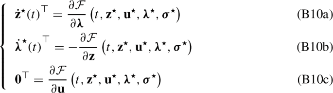
at each instant t of continuity of \(\textbf{u}^\star \), and the following transversal conditions hold:
$$\begin{aligned} {\varvec{\lambda }^\star }^\top (t_{\textrm{f}}) = - \frac{\partial J}{\partial \textbf{z}}(t_{\textrm{f}}, \textbf{z}^\star (t_{\textrm{f}})) \ . \end{aligned}$$(B11) -
(b)
the function \(\mathcal {H}(\textbf{z}^\star , \textbf{u}, \varvec{\lambda }^\star , t)\) defined in Eq. (B8) attains its maximum on \(\mathcal {U}\left[ t_{\textrm{i}}, t_{\textrm{f}}\right] \) at \( \textbf{u}(t) = \textbf{u}^\star (t)\) for every \(t \in [t_{\textrm{i}},t_{\textrm{f}}]\):
$$\begin{aligned} \mathcal {H}(\textbf{z}^\star , \textbf{u}^\star , \varvec{\lambda }^\star , t) \ge \mathcal {H}(\textbf{z}^\star , \textbf{u}, \varvec{\lambda }^\star , t) \ \quad \forall \ \textbf{u}(t) \in \mathcal {U}\left[ t_{\textrm{i}}, t_{\textrm{f}}\right] , \end{aligned}$$(B12)where \(\mathcal {U}\left[ t_{\textrm{i}}, t_{\textrm{f}}\right] \) is the class of admissible control functions defined in Eq. (15).

The adjoint differential equations, Eq. (B10b), originate from the Euler–Lagrange equations of optimal control (Longuski et al. 2014). For the present case, in a more explicit form, they are (superscript ‘\(\star \)’ is dropped to ease notation)

Concerning Eq. (B10c), the components of the vectorial algebraic equation are

The state and control variables that satisfy Eqs. (B10b) and (B10c) are termed extremals, for these solutions render the cost function an extremum (Hiday 1992). However, by the nature of the space trajectory problem, there is no upper bound to the fuel that could be consumed on a feasible trajectory. So, one may be confident that a solution is a local minimum and not a local maximum (Conway 2010).
Equation (B14c) requires either \(\sigma _1^\star \), \(q^\star \), or both should vanish. If \(q^\star = 0\), then, in accordance with Eq. (13), either \({{\,\mathrm{\text {T}}\,}}^\star = 0\) or \({{\,\mathrm{\text {T}}\,}}^\star ={{\,\mathrm{\text {T}}\,}}_{\max }\). If \(\sigma _1 ^\star = 0\), the thrust magnitude can assume intermediate values. Thus, the optimal trajectory may be comprised of the following types of arcs:
-
(i)
Null Thrust Arcs (NT-arcs) when \({{\,\mathrm{\text {T}}\,}}^\star = 0\),
-
(ii)
Intermediate Thrust Arcs (IT-arcs) when \(0< {{\,\mathrm{\text {T}}\,}}^\star < {{\,\mathrm{\text {T}}\,}}_{\max }\),
-
(iii)
Maximum Thrust Arcs (MT-arcs) when \({{\,\mathrm{\text {T}}\,}}^\star = {{\,\mathrm{\text {T}}\,}}_{\max }\).
Consider now Eq. (B14b). Provided that \(\sigma _2 ^\star \) and \({{\,\mathrm{\text {T}}\,}}^\star \) are both nonzero, \(\varvec{\alpha } ^\star \) and \(\varvec{\lambda }_v ^\star \) must be parallel. Let the adjoint vector to the velocity be termed the primer vector and, hereafter, be denoted as \(\textbf{p}(t) \equiv \varvec{\lambda }_v(t)\). Then, the optimal thrust direction is always parallel to the primer, and since \(\left\| \varvec{\alpha }^\star \right\| = 1\), \(\varvec{\alpha }^\star (t) = {\textbf{p}^\star (t) }/{\left\| \textbf{p}^\star (t)\right\| }\). The renaming of \(\varvec{\lambda }_v\) is not arbitrary, but rather this vector plays a relevant role in facilitating the understanding of optimal trajectories. If \({{\,\mathrm{\text {T}}\,}}^\star =0\), the motor is not operating, and the components of \(\varvec{\alpha }^\star \) are indeterminate; additionally, if \(\sigma _2^\star = 0\), the primer vanishes.
The optimal control is now chosen according to Pontryagin’s Maximum Principle stated in Eq. (B12), affirming that the Hamiltonian should be maximized over the choice of admissible control variables in order to minimize the cost function. Substituting the definition of \(\mathcal {H}\) reported in Eq. (B8) into Eq. (B12), utilizing the definition of the primer and simplifying,
Inequality Eq. (B15) is also recognized as the Weierstrass necessary conditions in calculus of variations, and it is the starting point employed by Lawden (1963). At each point on the optimal trajectory, Eq. (B15) must be valid for all the admissible values of \(\varvec{\alpha }\) and \({{\,\mathrm{\text {T}}\,}}\). Hence, Weierstrass inequality must be analyzed on each extremal of the optimal trajectory. The resulting conditions state that (Hiday 1992)
-
1.
whenever the thrust is operative and \(\left\| \textbf{p}\right\| \ne 0\), the thrust must act in the direction and sense of the primer vector
$$\begin{aligned} \varvec{\alpha } = \dfrac{ \textbf{p} }{\left\| \textbf{p}\right\| } \ ; \end{aligned}$$(B16) -
2.
defining thrust magnitude switching function S as
$$\begin{aligned} \mathcal {S}\, {:}{=}\, \dfrac{c\left\| \textbf{p}\right\| }{m} - \lambda _m \ , \end{aligned}$$(B17)then it is necessary that \(\mathcal {S}\le 0\) over an NT-arc, \(\mathcal {S}\ge 0\) over a MT-arc, and \(\mathcal {S}= 0\) over an IT-arc.
It remains to take into account Eqs. (B13c) and (B14a). They are employed to eliminate the adjoint \(\lambda _m\) from consideration, by expressing it in terms of the thrust magnitude switching function. Note that the superscript ‘\(\star \)’ will henceforth be dropped, and the subsequent states, controls and Lagrange multipliers are assumed to be evaluated on the optimal trajectory. Differentiating Eq. (B17) and solving for the derivative of the adjoint,
Equating the two expressions of \(\dot{\lambda }_m\) in Eqs. (B13c) and (B18) produces
Utilizing the conservation of mass expression in Eq. (11) for the term \(\dot{m}\) renders
which reduces to
Also, substituting Eq. (B17) into Eq. (B14a)
simplifying and rearranging
Hence, the constraints on the Lagrange multipliers \(\lambda _m\) and \(\sigma _1\) have been replaced by the specification of the switching function and its derivative according to Eqs. (B21) and (B23). On NT- and MT-arcs, Eq. (B23) serves only to determine the value of \(\sigma _1\). Since the spacecraft mass is constant on an NT-arc, Eq. (B21) is integrable to yield
Instead, on an IT-arc the conditions about \(\mathcal {S}\) further simplify. Recall that for an IT-arc, \(\sigma _1= 0\); therefore, from Eq. (B23), \(\mathcal {S} = 0\). In order for the switching function to remain zero throughout the duration of the IT-arc, the derivative of the switching function must also be identically zero. Accordingly, Eq. (B21) implies that \(\left\| \dot{\textbf{p}}\right\| = 0\) or \( \left\| {\textbf{p}}\right\| = \text {constant.}\)
The results of this section are now collected together. The necessary conditions for an optimal solution of Problem 1, which are also expressed by Theorem 1, can be stated in terms of the primer vector \(\textbf{p}\) and the thrust magnitude switching function \(\mathcal {S}\).
Proposition 3
(Necessary Conditions for a General Fuel-Optimal Trajectory) An optimal trajectory for Problem 1 is such that:
-
1.
Whenever the engine of the spacecraft is operative and \(\left\| \textbf{p}\right\| \ne 0\), the thrust must act in the direction and sense of the primer vector
$$\begin{aligned} \varvec{\alpha } = \dfrac{ \textbf{p} }{\left\| \textbf{p}\right\| } \ . \end{aligned}$$ -
2.
\(\mathcal {S}\) must respect the following specification on the three types of extremal arcs:
-
(i)
On a NT-arc, \({\mathcal {S}}\) is negative and is determined by Eq. (B24)
$$\begin{aligned} {\mathcal {S}} =\dfrac{c}{m}\left\| \textbf{p}\right\| + \textrm{constant} \quad \text {and} \quad {{\mathcal {S}}} \le 0 \ ; \end{aligned}$$ -
(ii)
On a MT-arc, \({\mathcal {S}}\) is positive and it respects Eq. (B21)
$$\begin{aligned} \dot{{\mathcal {S}}} = \dfrac{c}{m} \left\| \dot{\textbf{p}}\right\| \quad \text {and} \quad {{\mathcal {S}}} \ge 0\ ; \end{aligned}$$ -
(iii)
On an IT-arc, \({\mathcal {S}}\) is identically zero and the primer magnitude is constant
$$\begin{aligned} {{\mathcal {S}}}= \dot{{\mathcal {S}}} =0 \quad \text {and} \quad \left\| \dot{\textbf{p}}\right\| = 0 \ . \end{aligned}$$
-
(i)
Note that these conditions apply for either high- or low-thrust engines, as no assumption has been made on the thrust profile. Moreover, their validity holds irrespective of the astrodynamical model employed.
1.2 B.2 Primer differential equations in a four-body model
Writing Eq. (B13b) in terms of \(\textbf{p}\) and differentiating yields:
Then, substituting Eq. (B13a) inside Eq. (B25), simplifying and transposing, yields
Eq. (B26) is valid for every astrodynamical model, but in the framework of the PBRFBM, it reduces even more. Indeed, being \(\varvec{G_v}\) a constant matrix, \(\dot{\varvec{G_v}} \) is identically zero. Moreover, it was already pointed out that owing to the regularity of the effective potential \(\Omega \), \(\varvec{G_r}\) is symmetric. Thus, in the present case:
Furthermore, \(\varvec{G_v}\) is an antisymmetric matrix: \( -G_v^\top = G_v \). Hence, the second-order differential equation for the primer vector in a PBRFBM simplifies to
Lawden’s approach to the primer differential equation in the two-body problem results in a matrix \(\varvec{G_v}\) that is always zero (Lawden 1963). However, in the PBRFBM, the second derivative of the primer vector depends also on its first derivative. A notable advantage is that Eq. (B28) and Eq. (6) are actually the same second-order differential equation. Hence, the history of the primer vector in time can be computed by means of the STM (Lion and Handelsman 1968):
where \(\textbf{p}_{\text {i}} = \textbf{p}(t_{\text {i}})\), \(\textbf{p}_{\text {f}} = \textbf{p}(t_{\text {f}})\) are the values of the primer at the endpoints of the trajectory.
1.3 B.3 Impulsive thrust
Consider a high-thrust engine, which, for instance, employs conventional chemical propulsion. It is shown hereafter how this assumption simplifies the necessary conditions just found.
First, minimizing the fuel expenditure is equivalent to minimizing the characteristic velocity, i.e., the sum of the magnitude of the velocity changes (Longuski et al. 2014). Then, the duration of an arc of maximum thrust is negligible if compared to the total time of the mission. Accordingly, for the purpose of finding an optimal trajectory, the motion of the spacecraft during a MT-arc can be neglected. So, a MT-arc is approximated as an impulse useful to change the velocity of the spacecraft, without affecting its position. Lastly, the velocity change \(\left\| \Delta \textbf{v}\right\| \) is aligned to the thrust direction \(\varvec{\alpha }\) at the time of the impulse.
According to the calculus of variations terminology, a corner exists if an instantaneous change in the control variable (i.e., an impulse) causes some of the state variables to experience a discontinuity. The theorem that follows, from calculus of variations, outlines the conditions that must be met at the corner points of an optimal solution (Longuski et al. 2014).
Theorem 2
(Weierstrass–Erdmann Corner Conditions) Consider the fuel-optimal problem described in Problem 1, and suppose that the quadruple \(\left\{ \textbf{u}^\star , \textbf{z}^\star , \varvec{\lambda }^\star , \varvec{\sigma }^\star \right\} \) are associated with the optimal trajectory (i.e., they satisfy the necessary conditions reported in Theorem 1). At every corner point \(t_k \in (t_{\textrm{i}},t_{\textrm{f}})\) of \(\textbf{u}^\star (t) \in \mathcal {U}[t_{\textrm{i}},t_{\textrm{f}}]\), the following conditions must hold:
where \(\mathcal {H}\) is defined by Eq. (B8), and \(t_k^-\), \(t_k^+\) denote the time instant just before and after the corner, respectively.
Equation (B30) stipulate that the adjoint variables must be continuous at a corner. As a consequence, also the primer vector \(\textbf{p} \equiv \varvec{\lambda _v}\) must be continuous across the impulse \(\textbf{p}^- = \textbf{p}^+ \). Using the definition of \(\textbf{p}\), Eq. (B13b) becomes
The derivative of the primer is expressed solely in terms of the continuous adjoint variables \(\varvec{\lambda }_r\) and \(\textbf{p}\), and the matrix \(\varvec{G_v}\), which is a constant in the PBRFBM. Hence, another outcome of the Weierstrass–Erdmann corner conditions is that also the derivative of the primer must be continuous at a corner: \(\dot{\textbf{p}} ^- = {\dot{\textbf{p}}}^+ \). A further consequence, from Eq. (B21), is that the derivative of the switching function is continuous across the impulse: \(\dot{\mathcal {S}} ^- = \dot{\mathcal {S}} ^+\).
The second corner condition requires that the Hamiltonian is continuous across the discontinuity of the control variable. The Hamiltonian defined in Eq. (B8) can be rewritten in terms of \(\textbf{p}\) and \(\dot{\textbf{p}}\) by using Eq. (B13b)
As \({{\,\mathrm{\text {T}}\,}}\) is discontinuous at a corner, the only possibility for \(\mathcal {H}\) to be continuous is that
which, from the definition of \(\mathcal {S}\) in Eq. (B17), is equivalent to state that
To sum up, at a corner of an optimal trajectory \(\mathcal {S}\) and \(\dot{\mathcal {S}}\) are continuous and \(\mathcal {S} = 0\).
Leave aside for a moment the corner conditions and consider the following case where a NT-arc joins two impulsive thrusts. Let \(\text {P}\) denote the magnitude of the primer vector at the instant of one of the two maneuvers. Equation (B24) is valid over the entire NT-arc. Because at the arc boundaries \(\mathcal {S} = 0\) and \(\mathcal {S}\) is continuous, evaluating Eq. (B24) at an extreme point yields
The value of the constant is determined to be equal to \(-\dfrac{c}{m}\text {P}\), and Eq. (B24) becomes
From Eq. (B37), valid over the entire NT-arc, the magnitude of \(\textbf{p}\) must equal \(\text {P}\) at the other terminal as well (where still \(\mathcal {S} = 0\)). Hence, if an optimal trajectory is composed of NT-arcs separated by impulsive maneuvers, then \(\left\| \textbf{p}\right\| = \text {P}\) at every application of an impulsive thrust. If one or both of the impulsive maneuvers is replaced by an IT-arc, the previous conclusion is unaffected. Indeed, over an IT-arc, \({{\mathcal {S}}} = \dot{{\mathcal {S}}} = \left\| \dot{\textbf{p}}\right\| = 0\); therefore, an IT-arc on an optimal trajectory behaves exactly as an impulsive maneuver. Consequently, at all impulsive maneuvers and over all IT-arcs \(\left\| \textbf{p}\right\| = \text {P}\); also, over all NT-arcs \( \left\| \textbf{p}\right\| \le \text {P}\). The value of \(\text {P}\) can be computed applying the transversality conditions in Eq. (B11). According to Problem 1, the only state variable unspecified at the final time is the mass. The missing boundary condition for the final mass is
Using the definition of \(\mathcal {S}\) (Eq. B17), the final value of the switching function is
If the final arc of the trajectory is a NT-arc, Eq. (B37) can be evaluated at \(t=t_{\text {f}}\)
The value of the constant \(\text {P}\) is inferred comparing Eqs. (B39) and (B40), resulting in \(\text {P}= 1\). Alternatively, if the final arc is an IT-arc, then \(\mathcal {S}(t_{\text {f}}) = 0\) and Eq. (B39) is satisfied provided \(\left\| \textbf{p}\right\| = 1\). Recalling that \(\left\| \textbf{p}\right\| = \text {P}\) at every application of an impulsive thrust, the following conclusions can be drawn: on a fuel-optimal trajectory, the magnitude of the primer must not exceed unity on any NT-arc (where \(\mathcal {S} < 0\)), and, whenever the engine is operative, the primer is a unit vector aligned in the thrust direction \(\varvec{\alpha }\).
Now the second Weierstrass–Erdmann corner condition can be investigate further, to prove that at a corner also \(\dot{\mathcal {S}} =0 \). According to the result of Eqs. (B33) and (B34), the second corner condition \(\mathcal {H}^+ - \mathcal {H}^- = 0\) is
Regrouping terms and using that the primer and its derivative are continuous across the corner, the previous equation simplifies to
where the superscripts of \(\varvec{G_v}\) are removed as it is a constant matrix in the present case.
In the PBRFBM, the quantity \(\left( \textbf{g} - {\varvec{G_v}} \textbf{v}\right) \) is evaluated as
From the definition of the effective potential in Eq. (2), \(\Omega \) is a function only of the time t and the position vector \(\textbf{r}\). Similarly, its partial derivatives are dependent solely on the position coordinates of the spacecraft. As these are continuous across an impulsive maneuver, so does the quantity \(\left( \textbf{g} - {\varvec{G_v}} \textbf{v}\right) \). Thus, the corresponding term in Eq. (B42) vanishes, yielding to
where \(\Delta \textbf{v} = \textbf{v}^+ - \textbf{v}^-\) is the velocity discontinuity at the corner. As \(\left\| \Delta \textbf{v} \right\| \ne 0\) at an impulse, Eq. (B44) is satisfied either if \(\left\| \dot{\textbf{p}}\right\| =0\) or if \(\dot{\textbf{p}}\) and \(\Delta \textbf{v}\) are orthogonal each other. Recalling the first necessary condition stated in Proposition 3, the thrust direction, which in turn is parallel to \(\Delta \textbf{v}\), is aligned with the primer vector at the instant of the impulsive maneuver. Thus, Eq. (B44) is equivalent to
Remember also that the magnitude of \(\textbf{p}\) has been previously determined to equal unity at the instant of an impulsive maneuver. Then, Eq. (B45) is met when the derivative of the magnitude of the primer vector is zero at a corner. This concludes the proof of Proposition 1. \(\square \)
Rights and permissions
Open Access This article is licensed under a Creative Commons Attribution 4.0 International License, which permits use, sharing, adaptation, distribution and reproduction in any medium or format, as long as you give appropriate credit to the original author(s) and the source, provide a link to the Creative Commons licence, and indicate if changes were made. The images or other third party material in this article are included in the article's Creative Commons licence, unless indicated otherwise in a credit line to the material. If material is not included in the article's Creative Commons licence and your intended use is not permitted by statutory regulation or exceeds the permitted use, you will need to obtain permission directly from the copyright holder. To view a copy of this licence, visit http://creativecommons.org/licenses/by/4.0/.
About this article

Cite this article
Grossi, G., Buonagura, C., Giordano, C. et al. On optimal three-impulse Earth–Moon transfers in a four-body model. Celest Mech Dyn Astron 136, 22 (2024). https://doi.org/10.1007/s10569-024-10193-4
Received:
Revised:
Accepted:
Published:
DOI: https://doi.org/10.1007/s10569-024-10193-4