
Abstract
This work presents an up-to-date model for the simulation of non-stationary ground motions, including several novelties compared to the original study of Sabetta and Pugliese (Bull Seism Soc Am 86:337–352, 1996). The selection of the input motion in the framework of earthquake engineering has become progressively more important with the growing use of nonlinear dynamic analyses. Regardless of the increasing availability of large strong motion databases, ground motion records are not always available for a given earthquake scenario and site condition, requiring the adoption of simulated time series. Among the different techniques for the generation of ground motion records, we focused on the methods based on stochastic simulations, considering the time- frequency decomposition of the seismic ground motion. We updated the non-stationary stochastic model initially developed in Sabetta and Pugliese (Bull Seism Soc Am 86:337–352, 1996) and later modified by Pousse et al. (Bull Seism Soc Am 96:2103–2117, 2006) and Laurendeau et al. (Nonstationary stochastic simulation of strong ground-motion time histories: application to the Japanese database. 15 WCEE Lisbon, 2012). The model is based on the S-transform that implicitly considers both the amplitude and frequency modulation. The four model parameters required for the simulation are: Arias intensity, significant duration, central frequency, and frequency bandwidth. They were obtained from an empirical ground motion model calibrated using the accelerometric records included in the updated Italian strong-motion database ITACA. The simulated accelerograms show a good match with the ground motion model prediction of several amplitude and frequency measures, such as Arias intensity, peak acceleration, peak velocity, Fourier spectra, and response spectra.
1 Introduction
With the increase of computational power and the advent of performance-based earthquake engineering, nonlinear dynamic analyses in the time domain are more often employed for the seismic assessment of new and existing civil constructions, including strategic and base-isolated structures, high ductility and irregular structures, coupled soil-structure systems. In the last years, several databases containing many natural ground motion records were created and updated (Chiou et al. 2008; Bozorgnia et al. 2014; Luzi et al. 2016) and many authors proposed criteria and methods for the record selection (Katsanos et al. 2010; Iervolino et al. 2010a; Baker and Lee 2018). Nevertheless, as the number of ground motion records of strong earthquakes in near source conditions is still limited and they cannot always match the given scenarios, synthetic ground motions are often used in the evaluation of seismic demand of structures. The simulated ground motions must be compatible with a given design response spectrum and the assumed earthquake scenario, usually described in terms of magnitude, distance, site geological conditions and focal mechanism.
A detailed review of the different techniques for predicting earthquake ground motions for engineering purposes is provided in Douglas and Aochi (2008).
The filtering and windowing of white noise, as the classic stochastic stationary procedure of SIMQKE (Gasparini and Vanmarcke 1976) and the analysis of the nonlinear dynamic response in the Kanai-Tajimi model (Kanai 1961; Lin and Yong 1987) were particularly used in the past. These methods, based on the random-vibration theory (Boore and Joyner 1984), provide accelerograms whose response spectra match the target spectrum. The spectral matching procedures are carried out in the frequency domain using a power spectral density function, the selection of which is the key issue and represents the main difference among various generation procedures. The main weakness of this kind of approach is that the time series are stationary in frequency and completely unrelated to any geophysical parameter.
A second category of methods relies on physics-based deterministic methods, where the ground motion is modelled by convolving source, path, and site effects (Spudich and Hartzell 1985). The kinematic models characterize the rupture process in terms of fault displacement as a function of time and location. The response at the site is calculated convolving the source function with the Green’s functions that represent the ground motion deriving from a point dislocation at a specific position on the target fault. (Kamae et al. 1998; Hartzell et al. 2005). These methods require a detailed knowledge of the source rupture characteristics, and are limited in frequency, generally up to 1–2 Hz.
The dynamic models (where the rupture process is simulated by considering the stress conditions) represent a step up in complexity from kinematic models and have the advantage of proposing various possible rupture scenarios of different magnitudes for a given seismotectonic situation. They are based on the numerical solution of the elasto-dynamic equations in a discretised continuum and are represented by finite-difference and finite-elements methods (Smerzini and Villani 2012; Paolucci et al. 2018). The physics-based numerical simulations are also limited in frequency, demand high computational resources, and require a reliable 3D model that is hardly available in practice.
Another approach to ground motion simulation consists in stochastic methods (Hanks 1979; Hanks and McGuire 1981) that combine seismological models of the spectral amplitude of ground motion with the engineering notion that the high frequency motion is basically random. These methods grew out of the consideration that large part of the strong ground shaking, usually associated with the arrival of S waves, appears incoherent and essentially random in nature. Furthermore, the Fourier amplitude spectrum (FAS), predicted by the Brune (1970) source model and often observed in actual earthquakes, is approximately constant between the corner frequency fc and fmax (frequency at which the logarithm of the FAS starts to decay for increasing frequencies). The strong ground motion can be approximated by finite duration (arrival of S waves), band limited (fc − fmax) Gaussian white noise. Under this assumption, by fixing the spectral amplitude and then generating different arrays of phases (random numbers uniformly distributed between 0 and 2π) it is possible to simulate acceleration time series looking similar in the frequency content but different in the details. This method was originally developed by Boore (1983) and made popular by the Stochastic-Method SIMulation (SMSIM) computer code (Boore 2003). An extension to finite faults is represented by EXSIM, a stochastic finite-source simulation algorithm (Boore 2009; Atkinson and Assatourians 2014). The application of this kind of models requires the knowledge of several parameters characterizing the source process and the wave propagation. The variability of the motion is considered by the random phase generation and the frequency content is assumed stationary with time.
Some recent studies compare the impact of different techniques on the results of the final engineering analysis. Schwab and Lestuzzi (2007) carried out nonlinear analyses on single-degree-of-freedom (SDOF) systems using time-series produced by the stationary procedure of SIMQKE (Gasparini and Vanmarcke 1976) as well as semiempirical non-stationary stochastic simulations (Sabetta and Pugliese 1996). They show that the classic stationary procedure leads to a significant underestimation of the ductility demand compared to natural accelerograms, whereas the non-stationary procedure performs much better (Iervolino et al. 2010b).
Among the above listed techniques for generating accelerograms, in this study we focused on methods based on stochastic simulations, considering the time–frequency decomposition of the seismic ground motion (Laurendeau 2013; Causse et al. 2014; Hong and Cui 2020). We have chosen to update the non-stationary stochastic model initially developed by Sabetta and Pugliese (1996) and modified by Pousse et al. (2006) and by Laurendeau et al. (2012). This method has the advantage of being simple, fast, and considering the basic concepts of seismology (Brune's source model, realistic time envelope function, non-stationarity in frequency, ground-motion variability). The generation of the simulated accelerograms depends on few input parameters: moment magnitude, source to site distance, shear wave velocity in the uppermost 30 m at the site, and style of faulting. This means that the end-user needs to know only some basic parameters of the target earthquake scenario. The four model parameters required for the simulation are obtained from regression analyses on a strong motion dataset of shallow active crustal events in Italy (Lanzano et al. 2019) and are embedded in the simulation code: Arias intensity (IA), significant duration (DV), central frequency (Fc), and frequency bandwidth (Fb). The recent development of large strong-motion databases for Europe as the Engineering Strong Motion database ESM 2.0 (https://esm-db.eu; Luzi et al. 2020) and the ITalian ACcelerometric Archive ITACA 3.1 (http://itaca.mi.ingv.it; D’Amico et al. 2020), was a key motivation for the updating of the stochastic method. The purpose of this study is to provide the earthquake engineering community with an improved stochastic model for the simulation of non-stationary accelerograms, giving a good fit with the target response spectrum even for a small number of simulations. Time-domain simulations are derived from a time–frequency decomposition of the signal and depend on the above-mentioned parameters obtained from the Ground Motion Model (GMM) by Lanzano et al. (2019). It follows that the results presented herein are specific for Italy, although the approach is general and can be adapted to other databases if predictive equations for Arias intensity and significant duration are available.
2 Non-stationary stochastic ground motion model
We start from the model proposed by Sabetta and Pugliese (1996), hereafter SP96, a simulation of non-stationary time series based on the summation of Fourier series with random phases and time-dependent coefficients. The coefficients of the Fourier series are obtained from a frequency-time decomposition of the signal that, according to the definition given by Stockwell et al. (1996), is named S-transform. The S-transform provides frequency-dependent resolution with referenced phase information and the sum of the coefficients of the S-transform over time equals the Fourier coefficients. Unlike the continuous wavelet transform, the S-transform produces a time–frequency representation instead of a time-scale representation (Cui and Hong 2020).
The S-transform of a signal x(t), such as a ground-motion record, is defined as (Stockwell et al. 1996):
in which S(f,τ) is the S-transform of x(t), f and t are frequency and time, and τ is the center of the window function w(f, τ – t). A frequently selected window is a Gaussian function represented by:
in which κ is a parameter that controls the number of oscillations in the effective width of the window. In our application, we set κ equal to 1. The window width for a given κ is inversely proportional to the frequency. Figure 1 shows the application of the S-transform to the ground motion recorded at the station of CSC during the Central Italy earthquake (Mw = 6.5) of October 30, 2016. It can be noted as the high frequencies decrease with increasing time.

Application of the S-transform to the EW component of the ground motion recorded at the station of CSC during the central Italy earthquake (Mw = 6.5, RJB = 12.8 km, VS30 = 698 m/s) of October 30, 2016: a Strong motion record; b 3D S-Transform; c 2D S-Transform
If we take the square of the S-transform, it becomes a natural extension of the power spectrum to the non-stationary case and it is constituted by a series of Power Spectral Densities (PSDs), calculated at different times.
The function Xs(t,f) upgrades the frequency-time decomposition used in SP96 and called Physical Spectrum (PS) which had a moving time window represented by a Gaussian function with a fixed length of 2.5 s. The PSDs can be fitted with a lognormal function defined through three parameters derived from the theory of the spectral moments (Vanmarcke 1980; Lai 1982). These parameters are the average total power Pa, corresponding to the area under the PSD; the central frequency Fc, giving a measure of where the PSD is concentrated along the frequency axis; and the frequency bandwidth Fb, corresponding to the dispersion of PSD around the central frequency. By inserting the time dependence and substituting PSD with Xs(t,f), the definition of the spectral moments and of the relative parameters becomes:
where Pa(t), instantaneous average power, is the time envelope function describing the amplitude variation of the ground motion. Its integral in the time domain is equal to the integral of Xs(t,f) in the time–frequency plane and corresponds to the Arias Intensity (Arias 1970, hereafter IA) in cm2/s3 apart from the scale factor π/2 g:
Fc(t), central frequency, and Fb(t), frequency bandwidth, represent the non-stationarity of the frequency content and correspond, respectively, to the centroid of Xs and to the radius of gyration of Xs with respect to Fc in the frequency plane. With the above-defined parameters, it is possible to derive a lognormal function approximating Xs(t,f):
where β(t) and δ are derived from Fc(t) and Fb(t) in the following way:
Pousse et al. (2006) pointed out that a closer analysis of SP96 model shows three basic drawbacks:
-
1.
Deficit of energy in the low frequency part of the Fourier spectra of the simulated accelerograms. To overcome this problem, Pousse et al. (2006) proposed to use directly the Brune spectrum (ω-square model) modulated at high frequencies substituting fmax with the central frequency Fc(t). In fact, the adoption of their model, replacing the lognormal distribution in frequency adopted by SP96, does not allow the modulation with time of low frequencies and produces response spectra with unrealistic amplitudes at long periods. Furthermore, as pointed out by Laurendeau et al. (2012), the ω-square point-source model leads to an overestimation of the spectral amplitude at long periods for large magnitude events. Atkinson and Silva (2000) have shown that, despite its success in modeling high ground motions, the single-corner-frequency point source model overpredicts ground motions from moderate-to-large earthquakes at low-to-intermediate frequencies (0.1 to 2 Hz). To overcome the effective lack of low frequencies in SP96 model, generating lower values than expected in the simulated velocity and displacement time series, we adopted a modified function to approximate \(\widetilde{{X_{s} }}\left( {t,f} \right)\) in the frequency domain.
This function is equal to the lognormal function reported in Eq. 6 for f > fm and to the arithmetic mean of the lognormal function \(\widetilde{{X_{s} }}\left( {t,f} \right)\) and the ω − square Brune spectrum \({\Omega }\left( f \right)\) for f < fm, where fm is the frequency corresponding to the maximum value of the lognormal function.The Brune ω-square spectrum is defined as (Boore 2003; Pousse 2006):
$${\Omega }\left( f \right) = \frac{{\left( {2\pi f} \right)^{2} }}{{1 + (f/f_{c} )^{2} }}$$(8)$$\log_{10} f_{c} = 1.341 + \log_{10} \left( {\beta \left( {{\Delta }\sigma^{1/3} } \right)} \right) - 0.5M$$(9)where fc is the corner frequency, Δσ is the stress drop in bars, M is the moment magnitude, and β is the shear-wave velocity in kilometers per second. The adopted values are Δσ = 50 bars and β = 3.5 km/s (Bindi and Kotha 2020).
The modified function \(\widetilde{{X_{s} }}^{\prime}\left( {t,f} \right)\) is thus equal to:
$$\widetilde{{X_{s}^{^{\prime}} }}\left( {t,f} \right) = \left\{ {\begin{array}{*{20}l} {mean\left[ {{\Omega }\left( f \right), \widetilde{{X_{s} }}\left( {t,f} \right)} \right]} \hfill & { if\;f \le f_{m} } \hfill \\ {\widetilde{{X_{s} }}\left( {t,f} \right) } \hfill & {if\;f > f_{m} } \hfill \\ \end{array} } \right.$$(10)Figure 2 shows the fit of the spectral densities corresponding to the record of Fig. 1 at time t = 5 s, with the modified lognormal described above and derived from the spectral moments of the corresponding time history (Eq. 4). It is evident the increase in low frequency content respect to the former model of SP96 and the good fit of the modified lognormal with the PSD of the real record.
Fig. 2 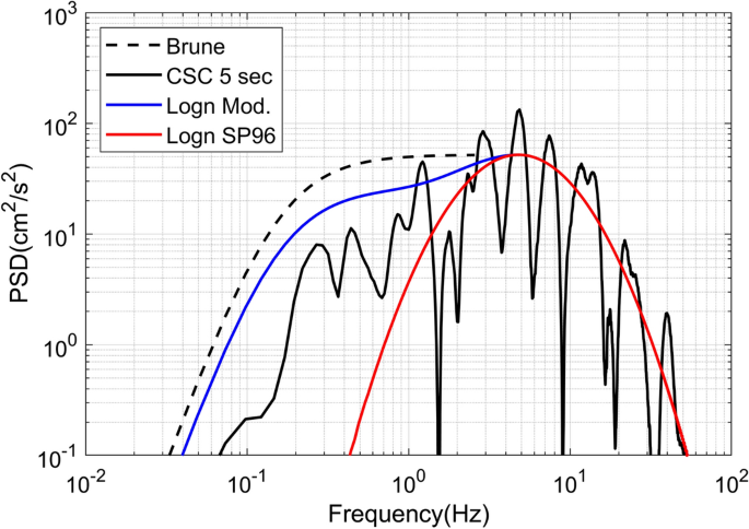
Fit of the PSD (squared Fourier transform of acceleration) corresponding to the record of Fig. 1 at time t = 5 s. with the original lognormal function adopted by SP96 (red line) and the modified function (Eq. 10) used in this work (blue line). For comparison, the normalized square of the Brune model calculated with the Eqs. (18) and (19) for Mw = 6.5 is also shown (dotted line)
-
2.
Envelope of simulated accelerograms. SP96 used a single-time envelope, Pa(t) in Eq. (4), for the whole time series. Pousse et al. (2006) considered, besides S waves, also P and coda waves. Even if this modification does not significantly change the energy distribution of the simulated accelerograms (in their model P waves amplitude is assumed 1/25 of S waves amplitude) we included their suggestion in our new model.
-
3.
Lack of variability in the simulated ground motion. Regarding the third problem detected by Pousse et al. in the original SP96 model, it is shown (Sect. 5—Table 3) that the difference among the simulated accelerograms given only by the introduction of the random phases, produces a variability, calculated as (max–min)/min, ranging from 60 to 150% in the Arias intensity and peak values. The coefficient of variation ranges between 7 and 19%, showing a lower variability respect to the natural accelerograms. However, we did not include further variability, e.g. considering the standard deviation of the values predicted by the GMM, in order to avoid an excessive dispersion of the results and to have a good match with the target response spectrum even for a small number of simulations. We considered a variability between 0 and 1 σ of the values foreseen by the empirical predictive equations only for the strong-motion duration that is not affected by the phase variability.

3 Ground-motion predictive models
3.1 PGA, PGV, acceleration response spectra, Arias intensity and Vanmarcke duration
A Ground Motion Model (GMM) for Italy has been recently calibrated by Lanzano et al. (2019), hereafter ITA18, with the aim of updating the existing GMMs for shallow active crustal regions in Italy (Bindi et al. 2011). The calibration dataset includes 5607 records, 146 events, and 1657 stations, from Italian and few well-sampled worldwide earthquakes in the magnitude range 3.5–8.0. The GMMs have been derived for the horizontal component (i.e. RotD50; Boore 2010) of Peak Ground Acceleration (PGA), Peak Ground Velocity (PGV) and of 36 ordinates of acceleration response spectra (SA) at 5% damping in the period range 0.01–10 s.
The functional form adopted by Lanzano et al (2019) is:
The source term, FM, the distance term, FD, and the site-effect term, FS, are:
a, b1, b2, c1, c2, c3, fj and k are the fixed coefficients obtained by a mixed-effects regression (Bates et al. 2015). The hinge Mh and the reference Mref magnitudes and the pseudo-depth h are pre-computed from a first stage nonlinear regression. The distance measure adopted is the closest horizontal distance to the vertical projection of the rupture as defined by Joyner and Boore, hereafter RJB (Abrahamson and Shedlock 1997). SOFj are the dummy variables for the Style Of Faulting (SOF) and the associated coefficients fj provide such correction. To discriminate among different focal mechanisms, we set j = 1 for strike-slip, j = 2 for reverse, and j = 3 for normal fault types. The coefficient for normal faulting is constrained to zero to perform the regression (f3 = 0).
The symbol ε in Eq. (11) represents the total residual associated with the median prediction. ε is decomposed in between-event, site-to-site, and event-and site corrected residuals (Atik et al. 2010), with standard deviation \(\tau\), \(\phi_{S2S}\) and \(\phi_{0}\), respectively. The total standard deviation \(\sigma\) can be computed as:
In the paper by Lanzano et al. (2019), the period-dependent hinge magnitude Mh in Eq. (12) is assumed as 5.5 at short periods in the range T = 0.01–0.4 s, Mh = 5.8 at intermediate to long periods (T = 0.45–5 s.) and Mh = 6.3 at periods longer than 5 s. However, the step between T = 0.4 s and 0.45 s causes unsmoothed shape of the predicted acceleration response spectra of events of moment magnitude around 6.0. To overcome such problem, we smooth the Mh bump from 5.5 to 5.8, using a stepwise variation of the hinge magnitude in a broader range of periods from T = 0.25 s to 0.7 s. The table of the re-calibrated coefficients and standard deviations is provided in the appendix.
The dataset used to derive ITA18 is also employed to calibrate the empirical equations to predict the horizontal component (RotD50) of the Arias Intensity computed as:
The functional form of IA is the same as Eq. (11), except for the source function FM, which is modified as:
We decided to adopt the quadratic scaling rather than the bi-linear, since it provides a better fit with data in this case. The coefficients of IA predictive equation and the associated standard deviations are shown in Table 1, in which some statistical indexes to verify the goodness of the fit are also reported. In addition to the standard error (SE), the p-value (Wasserstein and Lazar 2016) of the fixed coefficients is also included. Since only a coefficient with a p-value < 0.05 can be considered a meaningful contribution to the model, the correction for style of faulting (coefficients f1 and f2), shows a limited impact on predictions.
The total standard deviation associated to the prediction is 0.574, which is in line with the findings of Foulser-Piggot and Goda (2015), for Japanese data, and Sandikkaya and Akkar (2017), for European data, that are 0.596 and 0.560, respectively. The standard deviation is larger than the sigma obtained by SP96 (0.397), since their empirical relation was calibrated on a small number of observations compared to ITA18 dataset.
Figure 3 shows a comparison between the IA calibrated in this study and that estimated by SP96. For the sake of comparison, the latter has been scaled by a coefficient of 0.86 (Sabetta 2003) to convert the SP96 predictions, which represent the maximum between horizontal components, into RotD50. The ITA18 predictions are lower than SP96, and the difference increases with increasing source to site distance, a trend which has been already observed for other strong-motion parameters (e.g. PGA, PGV) and attributed to the limited data set of analog data used to derive SP96. To predict the significative duration of the ground motion, we did not use the definition of Trifunac and Brady (1975), corresponding to the interval between the achievement of 5 and 95% of the Arias intensity, because it tends to overestimate the duration in case of multiple shock recordings and it is not always well correlated to the strong part of the accelerogram. We preferred the DV definition given by Vanmarcke and Lai (1980) in its simplified formulation \({\text{DV = 7}}{.5}I_{A} /PGA^{2}\).

IA prediction obtained in this study compared with SP96 for rock sites (VS30 = 800 m/s), normal fault and two magnitudes (4.5 and 6.5). Observations are from the ITA18 database (Lanzano et al. 2019). The dashed thin lines represent the range corresponding to ± 1 standard deviation of the proposed model
This kind of duration is proportional to the ratio IA /PGA2 and is well correlated to the strong phase of the motion corresponding to the arrival of S waves.
Following Bommer et al. (2009), the empirical equations for the ground motion duration are calibrated using the same functional form of Eq. (8). The calibration results are given in Table 2. The p-values of the style of faulting coefficients are still the highest, confirming that the introduction of this explanatory variable in the model has a negligible impact on the standard deviation (Bommer et al. 2003; Lanzano et al. 2019). The total standard deviation (0.211) is comparable to that obtained by SP96 (0.247).
Figure 4 shows a comparison between DV predictions of ITA18 (this study) and SP96. The predictions of the two models are similar in near source conditions, while as the distance increases, ITA18 grows more than SP96, especially for low magnitude events.

Comparison between the prediction of SP96 and this study (ITA18) for rock sites (VS30 = 800 m/s), normal fault and two magnitudes (4.5 and 6.5). The dashed thin lines represent the range corresponding to ± 1 standard deviation of the proposed model
3.2 Central frequency Fc(t) and frequency bandwidth Fb(t)
Besides IA and DV, two further parameters must be calibrated over the data, i.e. the central frequency, Fc(t), and the frequency bandwidth, Fb(t) (Eq. 4).
To better constrain the predictive models and control the associated variability, ITA18 data are further skimmed considering a distance from the source lower than 50 km and a PGA greater than 0.03 g. This was done to eliminate noisy recordings with small amplitudes and long duration. Furthermore, the records that include secondary events have been excluded, since they produce anomalous trends of Fc and Fb with time. Despite the additional selection leads to the loss of more than 80% respect to the initial dataset (953 records vs 5607), the data still guarantee a good sampling in terms of Mw, RJB and VS30 as can be appreciated in Fig. 5.

Magnitude-Distance distribution of the data used in this study: white dots (5607 data) refer to the IA and DV calibration; red dots (953 data) refer to Fc and Fb calibration
Unlike IA and DV, Fc and Fb are extremely sensitive to the selected signal length as shown in Laurendeau (2013). Therefore, the accelerometric traces have been shortened in time using different percentages (5–95%, or 10–90%) of the Arias intensity. The first cut allows the signal to start approximately at the arrival of the P waves, while the second cut removes the tail of the signal that could contain surface waves or secondary events. The cut traces were then decimated to reduce the time sampling from 0.005 to 0.015 s. The S-transform of the signals was computed according to Eq. (1) and the fitting lognormal parameters according to Eq. (4).
Once Fc(t) and Fb(t) have been calculated for all the selected recordings, we got a dataset of more than 340,000 observations. Figure 6 provides the trend of log10(Fc) and Fb/Fc, which are the parameters required for the calculation of the lognormal function in Eq. (6), as a function of time, magnitude and VS30. Considering the scarce contribution of t > 45 s. for the simulation of waveforms, the data were furtherly cut out in time before the climb back up of Fc around 45 s shown in Fig. 6a.

Distribution of the parameters required for the calculation of the lognormal function: a–c = log10(Fc) as a function of a time, b moment magnitude and c VS30; Fb/Fc as a function of a time, b moment magnitude and c VS30
The data are affected by large uncertainties, but the median trends are comparable to those predicted by SP96: log10(Fc) decreases with time and magnitude, while increases with rising VS30. The time decay of Fb and Fc is similar, so that their ratio can be considered time independent, while a weak dependence on magnitude and VS30 is observed.
Laurendeau (2013) and Hong and Cui (2020) also showed that Fb and Fc data are affected by a large dispersion in the case of Japanese and NGA-West2 records, respectively, so that the predicting equations as a function of MW, RJB and VS30 suffer relevant uncertainties. For this reason, we performed several trial calibrations to define the optimal expressions. Figure 7 shows the behavior of Fc versus time obtained for different time windows, based on different fractions of Arias Intensity and length of the signal. Among the models illustrated in the figure, we adopted the one giving the best fit between the response spectra obtained with the simulations and those predicted by ITA18 (black line, that is intermediate between different models and providing the highest coefficient of determination R2).

Behavior of Fc versus time according to Eq. 16 and different IA and time interval selection in case of Rjb = 20 km, VS30 = 800 m/s and Mw = 6. In this study the black curve was adopted
The distance dependence of Fc(t) is taken into account shifting the Fc curve in time, according to the focal distance. Fc begins to decrease at time Tp when P waves arrive and remains constant after time Tcoda, denoting the arrival of the coda waves (Tp and Tcoda are defined in the following paragraph). Due to the large uncertainties in the Fc and Fb regressions and the weakness discussed previously of the statistical significance of the style of faulting coefficients for IA, and DV, we did not include a SOF coefficient in Fb and Fc predictive equations. The SOF dependence in the simulated time series is given by the coefficients included in IA, and DV regressions. The final predictive equations are the following:
where t = Tp if < Tp; t = Tcoda if > Tcoda
4 Time series simulation
After the evaluation of Pa (t, Mw, RJB, Vs30, SOF), Fc(t, Mw, Vs30), and Fb/Fc (Mw, Vs30), it is possible, for a given magnitude Mw, source-to-site distance (RJB or Repi), site condition VS30, and style of faulting SOF, to calculate an approximated \(\widetilde{{X_{s} }}^{\prime}\left( {t,f} \right)\) from Eq. (10).
The amplitude of \(\widetilde{{X_{s} }}^{\prime}\left( {t,f} \right)\) in the frequency domain is approximated by a modified lognormal function defined by Eqs. (6), (7), and (10).
The amplitude of \(\widetilde{{X_{s} }}^{\prime}\) in the time domain, Pa(t), represents the time envelope of the simulated accelerograms and, following Pousse et al. (2006), is defined by two lognormal followed by an exponential decay. In this way are considered the arrival time, energy, and broadening of the P and S pulses with distance, as well as the existence of scattered waves that produce the coda of the accelerogram. The shape of the P and S pulses is described by lognormal distributions truncated at time t = Tcoda and is prolongated by an algebro-exponential function simulating the coda waves according to the following formula:
In Eq. (21), the first term on the right-hand side corresponds to the P wave, the second represents the S wave, and the last one corresponds to the coda waves. Following Pousse et al. (2006), the coefficients 1/25 and 24/25 are based on the assumption that the body-wave amplitude from a double-couple point source varies in the far field as the velocity to the power of 3 (Lay and Wallace 1995). Since \(V_{P} /V_{S} = \sqrt {\left( {2{ } - { }2{\upnu }} \right)/\left( {1{ } - { }2{\upnu }} \right)}\), where ν is Poisson’s ratio, typically equal to 0.25 for geological materials (Kramer 1996), the Swave amplitude results about five times larger than the Pwave amplitude. µp, µs, σp, and σs are the expected mean values and standard deviations of the distribution of the parameter t for the P and S pulses, respectively. The parameters µp and µs control the time at which the maximum amplitudes of the P and S pulses are reached. Moreover, σp and σs characterize the broadening of the P and S pulses. For t ≥ Tcoda, Eq. (21) represents the coda waves decay (Aki and Chouet 1975). A0 is the source term representing the effect of both P and S waves; α is a parameter equal to 2 for body waves; Qc is the coda Q-value, assumed equal to QS under the hypothesis of a common wave attenuation mechanism for the S and the coda wave (Roecker et al. 1982). We adopted Qs = 250·f0.29 (Bindi and Kotha 2020). Figure 8 shows the graphical definition of the envelope function Pa(t) proposed in this study in comparison with that adopted in SP96.

Graphical definition of the time envelope function proposed in this study (red line) compared with that of SP96 (blue line) for Mw = 6.5, Rjb = 30 km and VS30 = 800 m/s
The time value indicated with Tsp corresponds to the time delay in seconds between S and P waves arrival and is calculated by dividing the focal distance Rhypo in kilometers by the factor Vp × Vs/(Vp—Vs) assumed to be equal to 7 km/s. Rhypo is calculated, for a depth given as input parameter, from the epicentral distance in turn obtained from RJB according to the procedure suggested by Scherbaum et al. (2004). The choices of Tp, Ts, Tcoda, σp, σs, were derived from several tests with real accelerograms to have a time envelope function Pa(t) with the following characteristics:
-
a modal value, at time t = Ts, correlated to the focal distance;
-
a standard deviation proportional to the strong-motion duration DV;
-
an area equal to the Arias intensity IA;
-
a total duration 30% greater than the value corresponding to the modal value plus 3DV.
Figure 9 shows, for a simulated accelerogram, the corresponding time envelope function Pa(t) and central frequency Fc(t).

a time envelope function Pa(t) proposed in this study in case of Mw = 6, Rjb = 20 km and VS30 = 800 m/s; b corresponding simulated accelerogram; c time behavior of the central frequency Fc(t)
The simulation of the accelerograms is then performed summing Fourier series with time-dependent coefficients derived from the approximated square of the S-transform \(\widetilde{{X_{S} ^{\prime}}}\) (Eq. 6) as follows:
where a(t) is the acceleration, f0 is the fundamental frequency (reciprocal of the total duration), and the phases φn are random numbers uniformly distributed in the range 0 to 2π. The computer code used for the time series simulation has been developed both in Fortran95 and Matlab. As shown in the flow-chart of Fig. 10, it requires as input parameters Mw, distance, focal depth, VS30, and SOF. The choice of the type of distance is constrained by the definition used in the reference GMM that is the fault distance RJB. However, it could be easier for engineers to use, the epicentral distance Repi as basic input parameter. Furthermore, this kind of distance, converted into focal distance, is required to build up the time envelope function Pa(t). Embedded in the code is the magnitude/SOF dependent conversion between Repi and RJB, according to the procedure suggested by Scherbaum et al. (2004). Also included in the code are the computations of IA, DV, Fc and Fb based on the predictive equations discussed in Sect. 3 and derived from the Italian database. The code produces as output acceleration, velocity, and displacement time series, Fourier spectra, response spectra, and a summary statistics of various measures of ground motion.

Flow-chart of the computer code used for the time series simulation
5 Results
Figure 11 shows nine simulated accelerograms in case of normal fault, VS30 = 800 m/s, RJB = 10 km, and MW = 5, 6, and 7. For each value of magnitude, three different simulations, differing only in the phase values, are plotted. The increase of magnitude causes an increase of amplitude, duration, and low-frequency content of the signal. The PGA of the simulated signals, reported on each time history, is close to the values predicted by the ITA18 GMM, that are equal to 46, 115 and 224 cm/s2 for the three values of magnitude, respectively. The attenuation of the simulated accelerograms with the distance from the source is represented in Fig. 12, in case of strike-slip fault, VS30 = 400 m/s, Mw = 6, and RJB = 10, 30, and 50 km, respectively. As expected, larger distances correspond to smaller accelerations and longer durations.

Simulated accelerograms in case of normal fault, VS30 = 800 m/s, RJB = 10 km, and a Mw = 5, b Mw = 6 and c Mw = 7. For each value of magnitude, three different simulations (a,b,c), differing only in the phase values, are plotted

Simulated accelerograms in case of strike-slip fault, VS30 = 400 m/s, M = 6, and RJB equal to: a 10, b 30, and c 50 km
Figure 13 shows the effect of different site conditions on the simulated time series of acceleration and velocity for normal fault, Mw = 6.5, RJB = 10 km, and VS30 equal to 400, 600, and 800 m/s, respectively. Going from soft to stiff soil, it is observed a decreased content of low frequencies, lower peak values, and a decrease in the duration of the time series.

Simulated time series of acceleration and velocity for Mw = 6, RJB = 10 km, normal fault, and VS30 respectively equal to a 400, b 600, and c 800 m/s
Figure 14 shows a comparison of the accelerogram recorded at the AQP station during an aftershock of the April 2009 L’Aquila earthquake (Mw = 5.4, RJB = 8.9 km, normal fault, VS30 = 836 m/s) with five different simulations in terms of acceleration. Figure 15 shows the same comparison in terms of velocity, displacement and Fourier spectrum.

Accelerogram recorded at AQP station during the L’Aquila earthquake (Mw = 5.4, RJB = 8.9 km, normal fault, VS30 = 836 m/s) of April 2009, compared with five different simulations in terms of acceleration

Accelerogram recorded at AQP station during the L’Aquila earthquake of April 2009 compared with a single simulation in terms of velocity, displacement, and Fourier spectra
The variability included in the simulated time-series only by the introduction of the random phases, is further illustrated in Table 3 for several scenarios in terms of magnitude distance and site conditions. The percentage variability of 100 simulations, calculated as (max–min)/min is around 60% for Arias Intensity, 120% for PGA, and 150% for PGV. The coefficient of variation is instead around 9% for Arias, 16% for PGA, and 17% for PGV. As discussed in Sect. 2, we assume this kind of variability as suitable for engineering applications. The value predicted by ITA18 is always between the mean value ± standard deviation of the simulations. Considering that the phase variation only acts on the peak values and that the selected definition of duration gives rather short durations compared to real records, we chose to add a uniform variation of DV between 0 and 1 standard deviation given by the regression equation. The effect of the DV variation is shown in the plots of Fig. 14.
Figure 16 shows a comparison of the Fourier spectra obtained from our model (mean of seven simulations) and the spectra derived from the Brune ω-square model defined in Eq. (8) and (9) with the addition of the high frequency cutoff and the geometrical and anelastic attenuation (Boore 1983) as:

Comparison among the Fourier Amplitude Spectra (FAS) of the mean of 7 simulated accelerograms and the spectra derived from the seismological ω-square Brune model for magnitudes 4.5, 5.5, 6.5, RJB = 30 km and VS30 = 800 m/s
C is a constant given by
where FS = 2 is the free surface correction, \(R_{\theta ,\varphi }\) = 0.63 is the average radiation pattern, and P = 1\(/\sqrt 2\) is the partition between the two horizontal components; ρ = 2.7 g/cm3 and β = 3.5 km/s are the density and S-wave velocity in the crust. M0 is the seismic moment derived from Mw (Hanks and Kanamori 1979). The corner frequency fc, defined in Eq. (9), is computed with a stress drop of 50 bars and the parameter k, controlling the high frequency decay, is set equal to 0.018. R is the distance (RJB) and Q is the quality factor, proportional to the frequency as: Q = Q0fn, where Q0 = 250 and n = 0.29. The values of the parameters adopted for the Brune model have been taken from Bindi et al. (2018) and Bindi and Kotha (2020).
The correspondence of the results obtained with very different models is remarkable, as shown in Fig. 16: the Brune’s ω-square model is theoretical and based, in the frequency domain, on the radiation of the seismic waves from a point source; the model of this study is empirical and based, in the time domain, on the statistical analysis of recorded strong ground motions.
Figure 17 compares the acceleration response spectra of seven simulated accelerograms with the 50-percentile spectrum predicted by ITA18. As comparison criterion we chose, in accordance with the Italian Seismic Code NTC18 (D.M. 2018) and the Eurocode EC8 (CEN 2009), a tolerance range of − 10% and + 30% with respect to the target spectrum. The red dotted lines in the figure correspond to the above-mentioned limits respect to ITA18. The black dashed lines represent the bound of ± one standard deviation of the seven simulations. The level of fit is quite satisfactory even for such a small number of simulations; the variability of the simulated spectra is only due to the different phases of the corresponding time series and does not include the uncertainty in the prediction of the ground-motion parameters used for the simulation. This is exactly the aim of this work: provide the engineer with a simulation method that, even with a small number of simulations, matches adequately the target response spectrum.

Response spectra of seven simulated accelerograms compared with the spectrum predicted by ITA18 GMM, in case of normal fault, MW = 5.5, RJB = 5 km, VS30 = 600 m/s;
The averaged response spectra resulting from twenty simulations are compared in Fig. 18 with the spectra predicted by ITA18 for different magnitudes, distances, and site conditions. The fit is satisfactory for all the considered cases.

Comparison of the mean response spectra derived from twenty simulated accelerograms, with the spectra predicted by ITA18 GMM for different: a, b, c magnitudes; d, e, f distances; g, h, i site conditions in case of a normal SOF
6 Simulation of time series in engineering applications
The selection of ground motions in the framework of earthquake engineering is becoming increasingly important with the growing use of nonlinear dynamic analyses, for which a set of input ground motions is a key component. The increasing availability of large strong motion databases pushes toward the use of natural accelerograms. However, natural records corresponding to the desired combination of magnitude, distance, soil type and SOF are not always available and appropriate spectral shapes cannot be achieved in case of excessive scaling (Causse et al. 2014). For these reasons, the relatively easy and fast generation of simulated records, compatible with an assigned design spectrum, is still very popular for both practice and research purposes (Iervolino et al. 2010b).
Given the little guidance provided in EC8 on how to select/generate code-compatible time-series, several articles have proposed sets of accelerograms consistent with the standard EC8 spectra (e.g. Giaralis and Spanos 2011; Iervolino et al. 2010b). Iervolino et al. (2010b) evaluated the nonlinear response of three types of SDOF systems applying different methods to generate artificial and simulated time series as well as scaled natural records.
Causse et al. (2014), to assess the variability in the response of engineering systems due to the differences in the simulated input motions, use the ground motion simulation method proposed by Laurendeau et al. (2012), very similar to the methodology proposed here, and compute the nonlinear response of SDOF systems by describing the hysteretic nonlinear behavior with the Takeda model. They show that the non-stationary stochastic approach of generating accelerograms is quite useful in capturing the true ground-motion variability and consequently the variability of building response.
To check the compatibility of the response spectra simulated with the method proposed in this study with the provisions of seismic codes, we compared the average spectra of 20 simulated ground motions with the spectral shapes given by the Eurocode EC8 (CEN 2009). Figure 19 shows the good agreement of the simulated spectra, normalized to their PGA, with the spectral shapes foreseen by EC8, type A soil, in case of high (Type 1) and low (Type 2) magnitudes. The Mw values of 7 and 5 correspond to those adopted (Sabetta and Bommer 2002) for the calibration of EC8 type 1 and 2, respectively.

Comparison of the mean of 20 simulated response spectra (normalized to the PGA) with a EC8 type 1 spectrum (Mw = 7, RJB = 5, VS30 = 800) and b EC8 Type 2 (Mw = 5, RJB = 30, VS30 = 800)
7 Conclusions
An improved stochastic model to generate nonstationary acceleration time series has been discussed in this paper. The development of the method is based on the S-transform and, unlike some of the models available in the literature, it considers the modulation both in amplitude and frequency. The amplitude modulation in time is obtained using time envelopes for the P, S, and coda waves. The frequency modulation is achieved with a lognormal function calibrated with the Brune’s ω-square model allowing for a realistic frequency content. The simulated time series depend on few input parameters: moment magnitude, source to site distance, shear wave velocity at the site, and style of faulting. The predictive equations for the response spectra are derived from the study of Lanzano et al (2019) with a calibration dataset including 5607 records, 146 events, and 1657 stations, from Italian and few well sampled worldwide earthquakes in the magnitude range 3.5–8.0. The same dataset has been used to derive the predictive equations for the most relevant parameters required for the time series simulation proposed in this study: Arias intensity and significant duration. The predictive equations for central frequency and frequency bandwidth have been derived from a reduced dataset calibrated to exclude records too far from the source, or too small, or including secondary events. The computer code implemented for the simulation, reproduces the non-stationarity in amplitude and frequency of the real ground motions, with promising applications in nonlinear dynamic analysis of structures. The simulated time series statistically fit the prediction of the ITA18 GMM for several ground-motion amplitude measures, such as Arias intensity, peak acceleration, peak velocity, Fourier spectra, and response spectra. The methodology proposed in this paper can be adapted to different databases provided that regional GMMs for Arias intensity and significant duration are available.
Availability of data and material
The updated table of ITA18 coefficients for Joyner-Boore distance is provided as supplementary electronic material.
Code availability
The code supporting the findings of the current study is publicly available in the Mendeley data repository with the identifier: https://doi.org/10.17632/vnsb4jgjgm.1.
Change history
19 April 2021
A Correction to this paper has been published: https://doi.org/10.1007/s10518-021-01102-3
References
Abrahamson N, Shedlock K (1997) Ground motion attenuation relationships. Seismol Res Lett 68(1):199–222
Aki K, Chouet B (1975) Origin of coda waves: source, attenuation, and scattering effects. J Geophys Res 80(23):3322–3342
Arias A (1970) A measure of earthquake intensity. In: Hansen RJ (ed) Seismic Design for nuclear power plants. MIT Press, Cambridge, pp 438–483
Atik LA, Abrahamson N, Bommer JJ, Scherbaum F, Cotton F, Kuehn N (2010) The variability of ground-motion prediction models and its components. Seismol Res Lett 81(5):794–801
Atkinson G, Silva W (2000) Stochastic modeling of California ground motions. Bull Seism Soc Am 90(2):255
Atkinson GM, Assatourians K (2014) Implementation and validation of EXSIM (a stochastic finite-fault ground-motion simulation algorithm) on the SCEC broadband platform. Seismol Res Lett 86(1):48–60
Baker JW, Lee C (2018) An improved algorithm for selecting ground motions to match a conditional spectrum. J Earthq Eng 22(4):708–723
Bates D, Mächler M, Bolker B, Walker S (2015) Fitting linear mixed-effects models using lme4. J Stat Softw 67(1):1–48
Bindi D, Kotha SR (2020) Spectral decomposition of the engineering strong motion (ESM) flat file: regional attenuation, source scaling and Arias stress drop. Bull Earthq Eng 18:2581–2606
Bindi D, Pacor F, Luzi L, Puglia R, Massa M, Ameri G, Paolucci R (2011) Ground motion prediction equations derived from the Italian strong-motion database. Bull Earthq Eng 9(6):1899–1920
Bindi D, Spallarossa D, Picozzi M, Scafidi D, Cotton F (2018) Impact of magnitude selection on aleatory variability associated with ground-motion prediction equations: part I. Bull Seism Soc Am 108(3A):1427–1442
Bommer JJ, Douglas J, Strasser FO (2003) Style-of-faulting in ground-motion prediction equations. Bull Earthq Eng 1(2):171–203
Bommer JJ, Stafford PJ, Alarcón JE (2009) Empirical equations for the prediction of the significant, bracketed, and uniform duration of earthquake ground motion. Bull Seism Soc Am 99(6):3217–3233
Boore DM (1983) Stochastic simulation of high-frequency ground motions based on seismological model of the radiated spectra. Bull Seism Soc Am 73(6A):1865–1894
Boore DM, Joyner WB (1984) A note on the use of random vibration theory to predict peak amplitudes of transient signals. Bull Seism Soc Am 74(5):2035–2039
Boore DM (2003) Simulation of ground motion using the stochastic method. Pure Appl Geophys 160(3–4):635–676
Boore DM (2009) Comparing stochastic point-source and finite-source ground-motion simulations: SMSIM and EXSIM. Bull Seism Soc Am 99(6):3202–3216
Boore DM (2010) Orientation-independent, nongeometric-mean measures of seismic intensity from two horizontal components of motion Bull. Seism Soc Am 100(4):1830–1835
Bozorgnia Y, Abrahamson NA, Atik LA, Ancheta TD, Atkinson GM, Baker JW, Darragh R (2014) NGA-West2 research project. Earthq Spectra 30(3):973–987
Brune J (1970) Tectonic stress and the spectra of seismic shear waves from earthquakes. J Geophyis Res 75(26):4997–5009
Causse M, Laurendeau A, Perrault M, Douglas J, Bonilla LF, Guéguen P (2014) Eurocode 8-compatible synthetic time-series as input to dynamic analysis. Bull Earthq Eng 12(2):755–768
CEN (2009) European Committee for Standardization, Eurocode 8: design of structures for earthquake resistance, Part 1: general rules, seismic actions and rules for buildings
Chiou B, Darragh R, Gregor N, Silva W (2008) NGA project strong-motion database. Earthq Spectra 24(1):23–44
Cui XZ, Hong HP (2020) Use of discrete orthonormal s-transform to simulate earthquake ground motions. Bull Seism Soc Am 110(2):565–575
D’Amico M, Felicetta C, Russo E, Sgobba S, Lanzano G, Pacor F, Luzi L (2020) Italian Accelerometric Archive v 3.1. Istituto Nazionale di Geofisica e Vulcanologia, Dipartimento della Protezione Civile Nazionale. https://doi.org/10.13127/itaca.3.1
D.M. (2018) Aggiornamento delle « Norme Tecniche per le Costruzioni » - D.M. 17/1/18 (in Italian)
Douglas J, Aochi H (2008) A survey of techniques for predicting earthquake ground motions for engineering purposes. Surv Geophys 29(3):187–220
Foulser-Piggott R, Goda K (2015) Ground-motion prediction models for Arias intensity and cumulative absolute velocity for Japanese earthquakes considering single-station sigma and within-event spatial correlation. Bull Seism Soc Am 105(4):1903–1918
Gasparini DA, Vanmarcke EH (1976) SIMQKE: a program for artificial motion generation. Department of Civil Engineering, Massachusetts Institute of Technology, Cambridge
Giaralis A, Spanos PD (2009) Wavelet-based response spectrum compatible synthesis of accelerograms Eurocode application (EC8). Soil Dyn Earthq Eng 29(1):219–235
Hanks TC, Kanamori H (1979) A moment magnitude scale. J Geophys Res 84(B5):2348–2350
Hanks TC (1979) b Values and ω−γ seismic source model: implication for tectonic stress variations along active crustal fault zones and the estimation of high-frequency strong ground motions. J Geophys Res 84(B5):2235–2242
Hanks TC, McGuire RK (1981) The character of high-frequency strong ground motion. Bull Seism Soc Am 71(6):2071–2095
Hartzell SH, Guatteri M, Mai PM, Liu P-C, Fisk M (2005) Calculation of broadband time histories of ground motion, part II: kinematic and dynamic modeling using theoretical green’s functions and comparison with the 1994 Northridge Earthquake. Bull Seism Soc Am 95(2):614–645
Hong HP, Cui XZ (2020) Time-frequency spectral representation models to simulate nonstationary processes and their use to generate ground motions. J Eng Mech 146(9):04020106
Iervolino I, Galasso C, Cosenza E (2010a) REXEL: computer aided record selection for code-based seismic structural analysis. Bull Earthq Eng 8(2):339–362
Iervolino I, De Luca F, Cosenza E (2010b) Spectral shape-based assessment of SDOF nonlinear response to real, adjusted and artificial accelerograms. Eng Struct 32(9):2776–2792
Lay T, Wallace TC (1995) Modern global seismology, international geophysics series, vol 58. Academic Press, San Diego
Kamae K, Irikura K, Pitarka A (1998) A technique for simulating strong ground motion using hybrid Green’s function. Bull Seismol Soc Am 88(2):357–367
Kanai K (1961) An empirical formula for the spectrum of strong earthquake 296 motions. Bull Earthq Res Inst 39:85–95
Katsanos EI, Sextos AG, Manolis GD (2010) Selection of earthquake ground motion records: a state-of-the-art review from a structural engineering perspective. Soil Dyn Earthq Eng 30(4):157–169
Kramer SL (1996) Geotechnical earthquake engineering, civil engineering and engineering mechanics. Prentice Hall, Upper Saddle River
Lai SP (1982) Statistical characterization of strong ground motions using power spectral density function. Bull Seism Soc Am 72(1):259–274
Lanzano G, Luzi L, Pacor F, Felicetta C, Puglia R, Sgobba S, D’Amico M (2019) A revised ground-motion prediction model for shallow crustal Earthquakes in Italy. Bull Seism Soc Am 109(2):525–540
Laurendeau A, Cotton F, Bonilla LF (2012) Nonstationary stochastic simulation of strong ground-motion time histories: application to the Japanese database. 15 WCEE Lisbon 2012
Laurendeau A (2013) Définitions des mouvements sismiques au rocher. PhD thesis, Université de Grenoble
Lin YK, Yong Y (1987) Evolutionary Kanai-Tajimi earthquake models. J Eng Mech 113(8):1119–1137
Luzi L, Puglia R, Russo E, D'Amico M, Felicetta C, Pacor F, Lanzano G, Çeken U, Clinton J, Costa G, Duni L, Farzanegan E, Gueguen P, Ionescu C, Kalogeras I, Özener H, Pesaresi D, Sleeman R, Strollo A, Zare M (2016) The engineering strong‐motion database: a platform to access pan‐European accelerometric data. Seismol Res Lett 87(4):987–997
Luzi L, Lanzano G, Felicetta C, D’Amico MC, Russo E, Sgobba S, Pacor F, ORFEUS Working Group 5 (2020) Engineering Strong Motion Database (ESM) (Version 2.0). Istituto Nazionale di Geofisica e Vulcanologia (INGV). https://doi.org/10.13127/ESM.2
Mark WD (1970) Spectral analysis of the convolution and filtering of nonstationary stochastic processes. J Sound Vib 11(1):19–63
Paolucci R, Infantino M, Mazzieri I, Ozcebe AG, Smerzini C, Stupazzini M (2018) 3D physics based numerical simulations: advantages and current limitations of a new frontier to earthquake ground motion prediction. The Istanbul case study. In: Pitilakis K (ed) Recent advances in Earthquake engineering in Europe. ECEE 2018. Geotechnical, Geological and Earthquake Engineering, vol 46. Springer
Pousse G, Bonilla L, Cotton F, Margerin L (2006) Nonstationary stochastic simulation of strong ground motion time histories including natural variability: application to the K-net Japanese database. Bull Seism Soc Am 96(6):2103–2117
Roecker SW, Tucker B, King G, Hatzfeld D (1982) Estimates of Q in central Asia as a function of frequency and depth using the coda of locally recorded events. Bull Seism Soc Am 72(1):129–149
Scherbaum F, Schmedes J, Cotton F (2004) On the conversion of source-to-site distance measures for extended earthquake source models. Bull Seism Soc Am 94(3):1053–1069
Schwab P, Lestuzzi P (2007) Assessment of the seismic non-linear behavior of ductile wall structures due to synthetics earthquakes. Bull Earthq Eng 5(1):67–84
Sabetta F (2003) Ground motion characterisation - elicitation summary. probabilistic seismic hazard analysis for swiss nuclear power plant sites (PEGASOS Project). Final report, vol 5, part IV, CD-ROM. Wettingen, July 2004, pp 338–422
Sabetta F, Bommer J (2002) Modification of the spectral shapes and subsoil conditions in Eurocode 8. In: 12th European conference on earthquake engineering, London, paper N° 518. Elsevier, Oxford. ISBN: 0080440495
Sabetta F, Pugliese A (1996) Estimation of response spectra and simulation of nonstationary Earthquake ground motions. Bull Seism Soc Am 86(2):337–352
Sandıkkaya MA, Akkar S (2017) Cumulative absolute velocity, Arias intensity and significant duration predictive models from a pan-European strong-motion dataset. Bull Earthq Eng 15(5):1881–1898
Smerzini C, Villani M (2012) Broadband numerical simulations in complex near-field geological configurations: the case of the 2009 Mw 63 L’Aquila earthquake. Bull Seismol Soc Am 102(6):2436–2451
Spudich PA, Hartzell SH (1985) Predicting earthquake ground-motion time-histories. US Geol Surv Profess Pap 1360:221–247
Stockwell RG, Mansinha L, Lowe RP (1996) Localization of the complex spectrum: the S transform. IEEE Trans Signal Process 44(4):998–1001
Stockwell RG (2007) A basis for efficient representation of the S-transform. Digit Signal Process 17(1):371–393
Trifunac MD, Brady AG (1975) A study on the duration of strong earthquake ground motion. Bull Seism Soc Am 65(3):581–626
Vanmarcke EH (1980) Parameters of the spectral density function, their significance in the time and frequency domain. MIT Civ Eng Des 60:1
Vanmarcke EH, Lai SP (1980) Strong-motion duration and RMS amplitude of earthquake records. Bull Seism Soc Am 70(4):1293–1307
Wasserstein RL, Lazar NA (2016) The ASA’s statement on p-values: context, process, and purpose. Am Stat 70(2):129–133
Acknowledgements
The authors would like to thank Francesca Pacor for the fruitful discussion in the preparation of this work, and the reviewers for the useful comments which significantly helped to improve and clarify the manuscript. Gabriele Fiorentino has received funding from the European Union’s Horizon 2020 research program under the Marie Curie grant agreement No. 892454 (https://cordis.europa.eu/project/id/892454/it). Giovanni Lanzano and Lucia Luzi are grateful to the European Research Infrastructure Consortium EPOS (European Research Infrastructure On Solid Earth) for the support in the development of the accelerometric databases ITACA and ESM.
Funding
European Union’s Horizon 2020 research program under the Marie Curie grant agreement No. 892454 (https://cordis.europa.eu/project/id/892454/it).
Author information
Authors and Affiliations
Corresponding author
Ethics declarations
Conflict of interest
The authors declare no conflict of interest.
Additional information
Publisher's Note
Springer Nature remains neutral with regard to jurisdictional claims in published maps and institutional affiliations.
Supplementary Information
Below is the link to the electronic supplementary material.
Rights and permissions
Open Access This article is licensed under a Creative Commons Attribution 4.0 International License, which permits use, sharing, adaptation, distribution and reproduction in any medium or format, as long as you give appropriate credit to the original author(s) and the source, provide a link to the Creative Commons licence, and indicate if changes were made. The images or other third party material in this article are included in the article's Creative Commons licence, unless indicated otherwise in a credit line to the material. If material is not included in the article's Creative Commons licence and your intended use is not permitted by statutory regulation or exceeds the permitted use, you will need to obtain permission directly from the copyright holder. To view a copy of this licence, visit http://creativecommons.org/licenses/by/4.0/.
About this article

Cite this article
Sabetta, F., Pugliese, A., Fiorentino, G. et al. Simulation of non-stationary stochastic ground motions based on recent Italian earthquakes. Bull Earthquake Eng 19, 3287–3315 (2021). https://doi.org/10.1007/s10518-021-01077-1
Received:
Accepted:
Published:
Issue Date:
DOI: https://doi.org/10.1007/s10518-021-01077-1