Modeling opponent learning in multiagent repeated games

Abstract

Multiagent reinforcement learning (MARL) has been used extensively in the game environment. One of the main challenges in MARL is that the environment of the agent system is dynamic, and the other agents are also updating their strategies. Therefore, modeling the opponents’ learning process and adopting specific strategies to shape learning is an effective way to obtain better training results. Previous studies such as DRON, LOLA and SOS approximated the opponent’s learning process and gave effective applications. However, these studies modeled only transient changes in opponent strategies and lacked stability in the improvement of equilibrium efficiency. In this article, we design the MOL (modeling opponent learning) method based on the Stackelberg game. We use best response theory to approximate the opponents’ preferences for different actions and explore stable equilibrium with higher rewards. We find that MOL achieves better results in several games with classical structures (the Prisoner’s Dilemma, Stackelberg Leader game and Stag Hunt with 3 players), and in randomly generated bimatrix games. MOL performs well in competitive games played against different opponents and converges to stable points that score above the Nash equilibrium in repeated game environments. The results may provide a reference for the definition of equilibrium in multiagent reinforcement learning systems, and contribute to the design of learning objectives in MARL to avoid local disadvantageous equilibrium and improve general efficiency.

1 Introduction

The interaction and learning process of multiple agents in game environments has been an important area of research. However, current learning algorithms for agents in noncooperative game environments usually lack generalization capabilities. Before the proposal of machine learning and reinforcement learning, this topic was usually discussed as part of game theory. The Theory of Learning in Games [1] summarized the early relevant results. It mainly consisted of the method of updating strategies using fictitious games [2] and the application of stochastic dynamical systems theory to explain the learning process [3]. SCE (self-confirming equilibrium) [4], as an extension of the Nash equilibrium, is usually considered the convergence result of this learning process [5]. Equilibrium selection theory [6] noted the core difference between the theory of learning and classical games: the existence of nonstationary equilibrium sets can serve as an asymptotic description for the long-term behavior of a system. Studies of this topic were usually based on equilibrium as well as convergence, but numerical experiments were difficult to perform due to technical limitations.

In recent studies, there have been good applications of deep reinforcement learning in multiagent systems [7], particularly in cooperation scenarios [8]. Agent communication has yielded many achievements in multiagent cooperative systems [9, 10]. The goal is to achieve the efficient operation of the system through higher-order communication between agents [11]. Another important area of multiagent cooperation is value function decomposition [12]. QMIX [13] combined with deep Q-learning has been successful in more complex tasks. It also inspired many subsequent works on value function decomposition [14, 15].

However, CTDE (centralized training decentralized execution) class algorithms [16, 17] can only be applied to cooperative tasks. For studies of competitive or mixed environments, progress is more concentrated around zero-sum games. A famous study concerned the AlphaZero algorithm [18], which beat the top human players in Go. The algorithm was able to learn the Nash equilibrium strategy in a complete information game. Texas Hold’em, as a typical example of an incomplete information game, was also solved with the introduction of the CFR (Counterfactual Regret Minimization) [19, 20] algorithm. Recent research includes the application of DMC (deep Monte Carlo) algorithms to solve the traditional Chinese game Fight the Landlord, which involves both cooperation and competition [21, 22].

Multiagent systems typically train strategies with repeated games. Unlike the single-agent environment, the reward received by each agent for taking an action in the game is influenced by the actions of other agents. Therefore, the difficulty is in making the learning process adapt to the non-Markovian environment [23] and avoid poorer local solutions [24]. Modeling other agents’ strategies is necessary when there are no shared targets or communication. DRON [25] is a method for estimating opponent strategies using historical samples, but its shortcoming is that it ignores changes in the opponent’s strategy. LOLA [26] was the first method to attempt to model and shape the learning process of opponents, and it had success in classical games such as the Prisoner’s Dilemma. This inspired subsequent work on opponent shaping (CGD [27] , COLA [28]). However, these algorithms focus only on transient changes in the opponent’s strategy and usually require all agents to adopt the same learning behavior. The advantages are that they are easy to implement and have good convergence guarantees for the Nash equilibrium. The problem is that short-term modeling may lead to local results such as an inferior Nash equilibrium. A balance between instantaneous rewards and opponent shaping is difficult to achieve.

In this paper, we design an algorithm based on MOL (modeling opponent learning), which uses best response theory to estimate the stable outcome of the opponent learning process and adopts specific strategies. MOL is executed in two phases. The goal of the first phase is to explore the opponent’s preferences for different actions, and the goal of the second phase is to learn stable equilibrium with higher rewards. We find that MOL has good convergence properties, and achieves good results in some classical games (the Prisoner’s Dilemma game, Stackelberg Leader game [29], Pennies matching game and Tandem game) as well as in randomly generated bimatrix games. Most of the algorithms that can be applied to two-agent games will fail in scenarios with more agents. However, in the multiagent Stag Hunt experiment we found that MOL can also be effective in scenarios with more than two agents. MOL also achieved higher average rewards in a competitive game environment and simultaneously improved the social welfare of the system. These experiments show that MOL improves over the original algorithms when dealing with diverse game environments or opponents.

The main contributions of this article are summarized as follows.

• This paper is the first to propose a MARL algorithm (MOL) from the perspective of modeling the long-term learning process of the opponent. MOL not only improves efficiency but also avoids using private information from other agents in the training process, which shows that the algorithm is efficient and generalizable.

• We provide theoretical support for the convergence results of the two stages of MOL. The reward of the stable outcome obtained by MOL will not be lower than a Nash equilibrium.

• For the first time, we introduce a competitive experiment in evaluating the MARL algorithm, where many algorithms based on opponent information cannot be applied. Our algorithm achieves good results in this experiment as well.

The remainder of this article is organized as follows. Section 2 introduces related works. Section 3 provides basic concepts about repeated games, learning systems, and opponent modeling to help explain the design of MOL. In Section 4, we describe in detail how the two stages of the MOL algorithm work. The experimental evaluation and results are discussed in Section 5. Finally, Section 6 concludes this work.

2 Related work

The application of reinforcement learning in decentralized multiagent systems has become a popular research area [30,31,32]. Algorithms applied to adaptive strategy learning in a noncooperative game environment have achieved remarkable success. The convergence of these algorithms in a general game environment were the main early results. WoLF (Win or Learn Fast) [33] successfully achieved the convergence of the Nash equilibrium in 2-dimensional matrix games. The AWESOME (Adapt When Everybody is Stationary, Otherwise Move to Equilibrium) [34] algorithm extended this result to the high-dimensional case. In both of these algorithms, convergence is achieved by starting from a stochastic initialization and improving the strategy in the direction of equilibrium. The Nash equilibrium has good stability and usually corresponds to dominant strategies. Therefore, these algorithms can learn the best response of a static opponent, and converge to the Nash equilibrium in self-play.

To cope with the diversity of opponent models in practical applications, theoretical research based on opponent modeling has made new progress. Unlike WoLF, these algorithms need to build a predictive model of the opponent’s strategy and select actions based on that model. DRON [25] based on DQN (deep Q-network) [35] was an early attempt to estimate the opponent’s strategy using neural networks [36, 37]. However, DRON has limitations because it cannot predict changes in the opponent’s strategy. The efficiency improvement over DQN is minimal, and the algorithm can only be applied in certain specific environments. Similar works have predicted the reward functions of other agents (bottom-up MARL) [38].

A number of subsequent studies attempted to model and shape the learning process of other agents. LOLA [26] is one of the works that have made landmark breakthroughs. By constructing a gradient algorithm based on a first-order differential approximation of the opponent’s strategy updates, LOLA achieves cooperation in the Prisoner’s Dilemma game. The SOS [39] (stable opponent shaping) algorithm combines LOLA with LookAhead [40] from the perspective of differential games to obtain better convergence results. The subsequent work COLA [28] improved this algorithm, and the core of its effectiveness is to guarantee the consistency of the agent’s estimation of the opponent’s learning process. Combining it with the trust domain algorithm MATRL [41], and the meta-game algorithm Meta-MAPG [42] has also yielded good results. This class of methods also includes SOM [43] and PGP [44]. All of these methods use the propagation of gradients with approximations to changes in the opponent’s strategy.

Although these algorithms have achieved good results in many game environments, we point out two aspects that could be improved. The first is that most of these approaches are based on a model of instantaneous changes in the opponent’s strategy, and the convergence result depends heavily on the consistency of higher-order lookahead. This makes the efficiency of the algorithm sensitive to the parameter settings, and the opponent’s strategy update process. In addition, gradient-based algorithms require the private information of other agents (the revenue matrix, strategies and even Hessain matrix). Using this information makes multiagent systems centralized or cooperative. This can lead to some restrictions on the environment in which the algorithm can be applied. Comparisons between prior algorithms and MOL are listed in Table 1.

Table 1 Comparisons between prior algorithms and MOL

3 Repeated game environments and agent learning systems

In this section, we present definitions of repeated games, agent learning systems, and optimization objectives. We also illustrate the design of MOL by comparing it with other algorithms.

3.1 Repeated games with learning systems

Different definitions of concepts such as a state and action space in MDP (Markov Decision Process) may lead to different results for the algorithm. Therefore, we will introduce the definition of a repeated game based on the Markov game.

A Markov game is specified by a tuple G =< S,U,P,R,O,n,γ >, which consists of n agents. In the current state s_i ∈ S, each agent chooses its own action a_i ∈ A. The obtained joint action u ∈ U leads to a state transition $P(s^{\prime }\vert s,u): S \times U \times S \rightarrow [0,1]$ and assigns different rewards rⁱ to each agent as well as the observation o_i ∈ O. γ ∈ [0,1) is the discount factor.

A repeated game can be viewed as the game above repeated as time $t \rightarrow \infty$. For round t of the game, the observation ${o^{i}_{t}}$ obtained by agent i is the joint action u_t as well as its own reward ${r^{i}_{t}}$ (the reward is private information). The state is ${s^{i}_{t}} \ = \ \bigcup \limits _{k=1, {\cdots } ,t}{o^{i}_{k}}$. To avoid an infinite increase in the dimension of the state space, we assume that ${s^{i}_{t}} \ = \ o^{i}_{t-1}$. For each agent, the state transition function is determined by the joint action composed of all agents and its own reward: $s^{i}_{t+1} = {o^{i}_{t}} = (u_{t},{r^{i}_{t}})$.

The general reinforcement learning algorithm is not applicable to the above non-Markovian game system because the state transition function is uncertain. The iteration process of the RL algorithm is a combination of the instantaneous reward and the reward expectation at the next moment:

$$ \begin{aligned} Q(s_{t}, a_{t}) \leftarrow \ & Q(s_{t}, a_{t})+\alpha[R_{t}(s_{t},a_{t})+\gamma \mathbb{E}[Q(s_{t+1}, \\ & a_{t+1}) ]-Q(s_{t}, a_{t})], \end{aligned} $$

(1)

where $s_{t+1} \sim P(s_{t},a_{t})$. However, in a multiagent system since the reward in each round is influenced by the actions of other agents ($A^{-}_{t}$), it becomes $\mathbb {E}\left [Q\left (s_{t+1}, a_{t+1}, A^{-}_{t+1}\right ) \right ]$. Even if we know $A^{-}_{t}$, $A^{-}_{t+1}$ may be unsolvable (because other agents are updating their strategies). If we consider a reward-independent repeated game (the reward depends only on joint actions), the above equation becomes:

$$ \begin{aligned} Q(a_{t}) = & R_{t}(a_{t} ,A^{-}_{t}) + \gamma \max_{A} \mathbb{E}[Q_{t+1} \\ & (A , A^{-}_{t+1}(a_{t}, A^{-}_{t}))], \end{aligned} $$

(2)

which is influenced by subsequent rewards (the strategies of other agents at the next moment $A^{-}_{t+1}=A^{-}_{t+1}(a_{t}, A^{-}_{t})$).

3.2 Strategies and equilibrium

There are two types of strategies: mixed and pure strategies. A mixed strategy is actually a distribution built on the set of actions A = {a₁,⋯ ,a_n}, denoted as:

$$ f \ : S \rightarrow F(A),F(A) = (p_{a_{1}},\cdots,p_{a_{n}}), $$

(3)

where $\sum p_{a_{i}} = 1$. A pure strategy can be seen as a special form of mixed strategy, where only one element in the action set (a_i) has a nonzero positive probability:

$$ p_{a_{i}} = 1 \ \text{and} \ p_{a_{j}} = 0 \ ,\text{for} \ j \neq i. $$

(4)

In this paper, we will train a pure strategy for the agent instead of a mixed strategy. This is because our algorithm is based on the exploration of the best response, which is a pure strategy in most cases. Modeling pure strategies can significantly reduce the dimension of the prediction space. Additionally, training mixed strategies requires gradient propagation in most cases, which uses the private information of opponents (the reward function or Hessian matrix) [45]. This article uses the same assumptions as in the AWESOME [34] algorithm: only the actions of all agents and their own rewards are observed. We also perform an analysis of the algorithm performance based on experiments in which only a mixed strategy equilibrium exists.

The equilibrium is used to characterize the stabilization point or convergence result in a game. The most important definition is the Nash equilibrium (NE), which is also the training objective of most algorithms. The NE is defined as a strategy combination such that each agent’s strategy is the best response to the other agents’ strategies. It is denoted as:

$$ f^{*} = (f^{*}_{1}, {\ldots} ,f^{*}_{n}), r^{i}(f^{*}_{i},f^{*}_{-i}) \geq r^{i}(f_{i},f^{*}_{-i}) \ f_{i} \neq f^{*}_{i}, $$

(5)

where $f^{*}_{-i}$ is the joint strategy of the agents other than agent i. Similarly, when all agents’ strategies are pure strategies and are the best responses to each other, we have:

$$ a^{*} = (a^{*}_{1}, {\ldots} ,a^{*}_{n}), r^{i}(a^{*}_{i},a^{*}_{-i}) \geq r^{i}(a_{i},a^{*}_{-i}) \ a_{i} \neq a^{*}_{i}, $$

(6)

and the joint action a^∗ is called a PSNE (pure strategy Nash equilibrium). In 1996, Athey proved that when a game satisfies the SCC (Single Crossing Condition), it has a PSNE [46].

Other approaches to strategy selection will lead to different equilibrium definitions, such as the correlated equilibrium and Pareto equilibrium. The application of the correlated equilibrium in meta-games [47] provided a good solver for multiplayer general-sum games.

In classical game theory, an important example of agent learning is the Stackelberg Leader game, which provides the possible convergence results when the agent knows that other players update their strategies by learning. It contributes to the promotion of cooperative behavior in repeated games [48].

According to the theory of the Stackelberg Leader game (the game structure is given in Table 2), when the row player knows that its opponent is engaged in a learning process, it will find that choosing action U will lead the opponent to an equilibrium (U,R), while choosing action D will lead to (D,L). Based on this consideration, the row player will choose U and thus ensure a reward of 3 for itself at convergence. This means that (U,R) is more reasonable as an equilibrium of an agent system with learning capability, although (D,L) is a unique Nash equilibrium point.

Table 2 Stackelberg Leader game

3.3 Optimization objectives

In this section, we introduce the optimization objectives of agents for different algorithms and give our motivation for designing algorithms based on the best responses.

For agent i in a repeated game, the predicted accumulated reward for action a_t is a combination of the instantaneous reward and subsequent reward expectations:

$$ \hat{Q}(a_{t}) = \mathbb{E}[R_{t}(a_{t} \vert \hat{A}^{-}_{t}) + \gamma \max_{A} R_{t+1}(A \vert \hat{A}^{-}_{t+1}) + \cdots] . $$

(7)

Since the opponents’ strategy $A^{-}_{t},A^{-}_{t+1}$ is updated, the agent needs to approximate the above optimization objective. A direct approximation is obtained by assuming that $\hat {A}^{-}_{t+m} \ (m>0)$ is independent of a_t, then we have:

$$ \mathop{\text{argmax}}\limits_{a_{t}} \hat{Q}(a_{t}) = \mathop{\text{argmax}}\limits_{a_{t}} \mathbb{E} [R_{t}(a_{t} \vert \hat{A}^{-}_{t})]. $$

(8)

The agent is optimized for instantaneous rewards, and it only needs to estimate the opponent’s current strategy. Both the INRL and LOLA algorithms are based on this assumption.

INRL [26] : This is also called a naive learner. The agent optimizes its own reward by choosing the best response, assuming that the opponent’s actions remain unchanged: $\hat {A}^{-}_{t} = {A}^{-}_{t-1}$. We take a 2-player game as an example. Assuming the joint action of agents 1 and 2 at the current moment t is (a_t,b_t), if agent 1 is a naive learner, then its action at t + 1 is

$$ a_{t+1} \ = \ \mathop{\text{argmax}}\limits_{a \in A} r^{1}(a,b_{t}). $$

(9)

If we take moment t as a starting point and assume that the opponent is also undergoing a learning process, then INRL optimizes the reward at moment t + 0 (when the opponent has not changed).

LOLA, SOS, COLA : This class of algorithms is based on the premise that the opponents are also updating their strategies, so that when the moment shifts from t to t + 1, the agent needs to estimate the changes in the opponents’ strategies and predict the next joint actions. We assume that at moment t the strategy $f({\theta ^{1}_{t}})$ of agent 1 is controlled by a parameter ${\theta ^{1}_{t}}$ and agent 2’s strategy $f({\theta ^{2}_{t}})$ is controlled by ${\theta ^{2}_{t}}$. Then, at the next moment t + 1, the strategy parameter of agent 2 will become

$$ \theta^{2}_{t+1} \ = \ {\theta^{2}_{t}} \ + \ {\Delta} \theta^{2}. $$

(10)

Therefore, if agent 1 wants to optimize its reward at the next moment, its strategy parameter should become

$$ \theta^{1}_{t+1} \ = \ \mathop{\text{argmax}}\limits_{\theta^{1}} R^{1}(\theta^{1},{\theta^{2}_{t}} + {\Delta} \theta^{2}). $$

(11)

LOLA implements this training process by assuming that the opponent is a naive learner and using the first-order approximation of Δ𝜃²:

$$ {\Delta} \theta^{2} = \nabla_{\theta^{2}}R^{2}(\theta^{1},\theta^{2})\cdot \eta, $$

(12)

(where η is a constant), which achieves good results in the Prisoner’s Dilemma game. As we can see from the previous discussion, the LOLA class algorithm considers the reward at moment t + 1 as the optimization objective (when the opponent has changed its strategy according to its learning process).

The above algorithms consider only instantaneous rewards and ignore the effects of actions on other agent strategies. Since estimating the opponent’s strategy at each subsequent moment is a complex process, we can derive a stable point of the strategy change process with best response theory.

Best Response : The best response is an important reference for agents when making strategic choices. It has good properties: the best response allows us to obtain the maximum reward when the agent has a known opponent strategy. If in a joint action, (a,b) ∈ A × B, both actions are the best response to the other action, that is:

$$ a \ = \ \mathop{\text{argmax}}\limits_{a^{\prime} \in A} r^{1}(a^{\prime},b) \quad b \ = \ \mathop{\text{argmax}}\limits_{b^{\prime} \in B} r^{2}(a,b^{\prime}), $$

(13)

then the PSNE has been reached.

The best response is also connected to the fixed point of learning. If there exists T₁ and $A^{-}_{t} \equiv A^{-}_{0}$ for t > T₁, then the agent’s strategy will converge to its best response.

$$ \lim_{t \rightarrow \infty} [a_{t} \vert (A^{-}_{t} \equiv A^{-}_{0})] = \mathop{\text{argmax}}\limits_{A} r^{1}(A,A^{-}_{0}). $$

(14)

When the discount factor γ is not sufficiently small, we can give an approximation of the accumulated reward:

$$ \begin{aligned} \hat{Q}(a_{0}) & = R(a_{0} \vert A^{-}_{0}) + \gamma R(a_{0} \vert A^{-}_{0}) + {\cdots} \\ & = (1+\gamma+\gamma^{2}+\cdots) R(a_{0} \vert A^{-}_{0}), \end{aligned} $$

(15)

where $A^{-}_{0}$ is the joint best response (BR) according to a₀. Then we have

$$ \mathop{\text{argmax}}\limits_{a_{0}} \hat{Q}(a_{0}) = \mathop{\text{argmax}}\limits_{a_{0}} R(a_{0} \vert A^{-}_{0}), \ A^{-}_{0} = BR(a_{0}). $$

(16)

Without restricting the learning rate δ, we can define the best response as the opponent strategy at moment $\infty$. Therefore, modeling the best response of the opponent can be seen as optimizing the reward at moment $t+\infty$.

4 Modeling opponent learning with two phases in multiagent repeated games

To implement the modeling and shaping of the opponent learning process, we design an algorithm named MOL (Modeling Opponent Learning). It can be divided into two phases. In the first phase, the agents optimize the instantaneous reward to explore the game structure as well as the best response of the opponent. In the second phase, the agents guide the learning process of the opponent to a stable point with a higher fixed reward.

4.1 Phase $\uppercase \expandafter {\romannumeral 1}$ of MOL

Phase I of MOL (MOL-1) starts from a random initialization, where the agent does not have any information about the game structure or the opponent. Thus, the objective of MOL-1 is to explore the game structure and the opponents’ preferences for different actions. We denote the opponents’ joint action at moment t as $a^{-}_{t}$. At the end of each round of the game, the agents are able to observe the joint action $(a_{t},a^{-}_{t})$ and their own rewards $r_{i}(a_{t},a^{-}_{t})$. In the first phase we create a Q-table to record the rewards for taking a certain action when the opponents’ action is fixed (approximating the structure of the reward matrix for each agent). We denote the agent’s expected reward as $\hat {q}(a \vert a^{-})$ for taking action a when the opponents are determined to take action a⁻, and we denote the actual value by r(a|a⁻).

Lemma 1

$\hat {q}(a \vert a^{-}) \rightarrow r(a \vert a^{-}), \forall a \in A, a^{-} \in A^{-} \text {as} \ t \rightarrow \infty$.

Proof

Denote N(a,a⁻) as the number of times the trajectory passes s(a,a⁻), then

$$ \forall a \in A, a^{-} \in A^{-}, N(a,a^{-}) \rightarrow \infty. $$

(17)

$$ \begin{aligned} &\hat{q}_{i+1}(a \vert a^{-}) \\ &= \hat{q}_{i}(a \vert a^{-}) + \delta(r(a,a^{-})-\hat{q}_{i}(a \vert a^{-})) \\ &=\delta r + (1-\delta)\hat{q}_{i}(a,a^{-}) \\ &=\delta r + (1-\delta)(\delta r +(1-\delta)\hat{q}_{i-1}(a \vert a^{-})) \\ &=\delta(1+(1-\delta)+{\cdots} )r(a,a^{-}) + (1-\delta)^{n} \hat{q}_{0} \\ &\rightarrow r(a,a^{-}) \quad n \rightarrow \infty \end{aligned} $$

(18)

which implies $\hat {q}(a \vert a^{-}) \rightarrow r(a \vert a^{-})$, thus Lemma 1 holds. □

We implement this process using the following approach: Before round t, the agent predicts the opponents’ actions $\hat {a}^{-}_{t}$ based on the previously tracked information (taking a greatest-likelihood approach). Then, the agent chooses the best response based on $\hat {q}$ and $\hat {a}^{-}_{t}$. We assume that the set of joint actions corresponding to the PSNE is U₀ ⊂ A₁ ×⋯ × A_n, then the prediction convergence set is $\hat {U}_{0} \subset \hat {A}_{1} \times {\cdots } \times \hat {A}_{n}$.

Lemma 2

Assuming that random exploration rate $\gamma \rightarrow 0$ as the number of iterative steps increases (γ ≈ 0 when T > N). The joint action U_t converges to PSNE set U₀, when at moment t(> N) agents’ joint prediction of the opponent’s action is in $\hat {U}_{0}$.

Proof

We assume that $(a_{0},a^{-}_{0})$ is a PSNE. According to Lemma 1 we know that the Q-table eventually converges to the true reward matrix $\hat {q}_{t}(a \vert a^{-}) \rightarrow r(a \vert a^{-})$. Then we have

$$ a_{0} = \mathop{\text{argmax}}\limits_{a^{\prime} \in A} r(a^{\prime} \vert a^{-}_{0}) = \lim_{t \rightarrow \infty} \mathop{\text{argmax}}\limits_{a^{\prime} \in A} \hat{q}_{t}(a^{\prime} \vert a^{-}_{0}). $$

(19)

Assuming that the prediction of joint action is the same for all agents as $\hat {u}_{0} = (\hat {a}_{1},\cdots ,\hat {a}_{n}) \in \hat {U}_{0}$ after the t th step. At this time ∀i = 1,⋯ ,n,

$$ \lim_{t \rightarrow \infty} \hat{a}^{-i}_{t} = (a^{-i}_{0}) \implies \lim_{t \rightarrow \infty} {a^{i}_{t}} = BR(a^{-i}_{0}) = {a^{i}_{0}}. $$

(20)

Similarly we have

$$ \lim_{t \rightarrow \infty} a^{-i}_{t} = a^{-i}_{0}. $$

(21)

Thus we prove that the convergence of the prediction is a sufficient condition for the convergence of the actual joint action. Considering that

$$ \hat{a}^{-i}_{t} = (a^{-i}_{0}), a^{-i}_{t} = a^{-i}_{0} \implies \hat{a}^{-i}_{t+1} = (a^{-i}_{0}), $$

(22)

therefore it is also a necessary condition. At moment t we assume that exploration rate γ ≈ 0, and every agent’s prediction is corresponding to a PSNE u₀ = (a₁,⋯ ,a_n). Then s_t+ 1 = u_t = u₀ and the prediction is unchanged. So the joint action converges to u₀ ∈ U₀. □

In the MOL-1 period we also want to explore the learned best response of the opponent when the agent takes different actions. Therefore, we need to increase the frequency of corresponding nonequilibrium actions. Our approach is to use the UCB (upper confidence bound) [49] function and to focus on exploration at the beginning of the training process. The UCB was chosen as the sampling function because of its ability to improve the exploration rate compared to the EI (expected improvement), and PI (probability of improvement), and thus allow for more accurate estimations of the best responses of other agents. The action of an agent at moment t is selected by:

$$ a_{t} = \mathop{\text{argmax}}\limits_{a \in A} (q_{t}(a \vert \hat{a}^{-}_{t}) + \sqrt{\frac{2\ln N}{n_{a}}}), $$

(23)

where N denotes the total number of rounds and n_a denotes the number of rounds in which the agent takes action a.

We give a proof of the algorithm’s convergence only for games with 2 players, due to a nice property of such games: when there are both pure and mixed strategy equilibrium in the game, there must be a linear combination relationship between them. Most existing algorithms, such as DRON, LOLA, and SOS, are based on the background of two-player games. Additionally, solving the Nash equilibrium for multiplayer general-sum games is an unsolved problem.

In the proof, we use the definition of the inferior action: if for two actions a and b, regardless of the opponent action, the reward for action a is never higher than that of b, then a is said to be an inferior action.

Lemma 3

When there exists a unique pure strategy Nash equilibrium (a,b), then for at least one of the agents it can obtain the action corresponding to the equilibrium (a) by repeatedly eliminating the inferior action.

Proof

First, in a 2-dimensional bimatrix game, we may assume that the unique pure strategy equilibrium is (L,U), and that the other optional actions are (R,D). Since (L,U) is a Nash equilibrium, the game has an equivalent matrix form as in Table 3, where M ≥ 0 and N ≥ 0.

Table 3 Bimatrix game with a unique PSNE

Since (L,U) is the only pure strategy equilibrium, c ≥ a and d ≥ b cannot be both true (otherwise (R,D) is also a Nash equilibrium). It may be assumed that c < a, then, D is an inferior strategy for the row player, and the action under equilibrium can be obtained by eliminating the inferior strategy. For the case in which the agent has more than two possible actions, we can obtain the elimination method similarly using the dominance relation of the action combination. □

Theorem 1

MOL-1 converges to Nash equilibrium in games with 2 players.

Proof

• When there is a unique pure strategy Nash equilibrium of the game, we may assume that (a,a⁻) is the PSNE, and let b = a⁻. From Lemma 3 we can see that there must be an agent at this time, remembered as agent 1. When the set of its available actions is A^∗ (A^∗ is derived by eliminating the inferior strategy of A), for each b ∈ B^∗, a is the best response of b. From Lemma 1 we have $\hat {q}_{t}(a,b) \rightarrow r(a,b)$, which indicates

  $$ \begin{array}{lllll} \forall b \in B^{*}, \ \hat{q}_{t}(a,b) \ge \hat{q}_{t}(a^{\prime},b) \ (\forall a^{\prime} \in A^{*} , t \rightarrow \infty). \end{array} $$

  (24)

  At this point, regardless of the value of $\hat {b}$, we have $\hat {q}_{t}(a,\hat {b})= \mathop {max}\limits _{a^{\prime } \in A^{*}}\hat {q}_{t}(a^{\prime },\hat {b})$. Thus, when $t \rightarrow \infty$, the action of agent 1 will converge to a. Then for agent 2, the opponent’s action prediction $\hat {a}$ will converge to a. And (a,b) is a PSNE, so

  $$ \hat{q}_{t}(b,\hat{a}) = r(b,a) = \mathop{max}\limits_{b^{\prime} \in B^{*}}\hat{q}_{t}(b^{\prime},\hat{a}). $$

  (25)

  Then the action of agent 2 will converge to b, which implies MOL-1 converge.

• When game has more than one PSNE, we want to prove that it will converge to one PSNE with probability 1 (as $t \rightarrow \infty$). We assume that γ ≈ 0 when t > T. The action of agent 1 is selected by $\mathop {max}\limits _{a \in A}q_{t}(a,\hat {b}) = \max \limits _{a \in A}r(a,\hat {b})$ from Lemma 1. We consider the set of pure strategy Nash equilibrium U₀ = {(a₀,b₀),(a₁,b₁),⋯ }⊂ A × B. When the joint prediction $p_{t}=(\hat {a}_{t},\hat {b}_{t})= (a_{i},b_{i}) \in U_{0}$, from Lemma 2 we have u_t+ 1 = (a_i,b_i), and $(\hat {a}_{t+1},\hat {b}_{t+1})= (a_{i},b_{i})$, which means when $(\hat {a}_{t},\hat {b}_{t}) \in U_{0}$ algorithm reaches a fixed point. We assume that the unstable point set is the complementary set $\overline {U_{0}}$, and there exists T₀, Q = R when t > T₀ for all players. And we assume that there exists T > T₀, p_T = (a_i,b_i) while p_T+ 1 = (a_j,b_j) i≠j. Since p_T is solved by using the previous track sample for the maximum likelihood, $\hat {a}_{T} \neq \hat {a}_{T+1} \Rightarrow N^{T}_{a_{i}} = N^{T}_{a_{j}}$ ($N^{T}_{a_{i}}$ means total number of occurrences of a_i before moment T).

  $$ \begin{aligned} p_{T} & = (a_{i},b_{i}) \ \text{and} \ p_{T+1} = (a_{j},b_{j}) \\ & \Rightarrow N^{T}_{a_{i}} = N^{T}_{a_{j}} \ \text{and} \ N^{T}_{b_{i}} = N^{T}_{b_{j}}. \end{aligned} $$

  (26)

  Due to the presence of random exploration in the algorithm controlled by the UCB function, we have

  $$ \lim_{t \rightarrow \infty} p (N^{t}_{a_{i}} = N^{t}_{a_{j}} \ , \ N^{t}_{b_{i}} = N^{t}_{b_{j}}) = 0. $$

  (27)

  Thus the joint action will not cycles between multiple pure strategy equilibrium. Considering that (a_i,b_j) or (a_j,b_i) are not available as a result of the convergence of the algorithm, we only need to exclude the case where the state cycles between non-stable points. For the case $\hat {u}_{t}=(a_{i},b_{j})$, there exists a minimum n satisfying $\hat {u}_{t+n}\neq (a_{i},b_{j})$. Similarly to equation (29) we have

  $$ \lim_{t \rightarrow \infty} p (\hat{a}_{t} \neq \hat{a}_{t+1} \ , \ \hat{b}_{t} \neq \hat{b}_{t+1}) = 0. $$

  (28)

  So we can assume that $\hat {u}_{t+n}=(a_{i},b_{m})$. Considering that random exploration rate $\gamma \rightarrow 0$ and b_i is the best response for a_i, we have

  $$ \hat{u}_{t},\cdots,\hat{u}_{t+n-1}=(a_{i},b_{j})\implies b_{t},\cdots,b_{t+n-1} = b_{i}, $$

  (29)

  which implies $b_{m}=b_{i}, \ \hat {u}_{t+n}=(a_{i},b_{i})\in U_{0}$. Thus we prove that the joint prediction converges to the set corresponding to PSNE. So when $t \rightarrow \infty$ the joint action will reach PSNE set U₀ with probability 1, which implies MOL-1 converge.

• In the previous discussion of the strategy section we mentioned that for each agent in a mixed equilibrium, its optional actions correspond to an identical reward. Thus for a game in which there is no pure strategy equilibrium (the existence of a mixed equilibrium is proved by the existence of NE), the corresponding set of joint actions is $A^{\prime } \times B^{\prime }$. For agent 1, when $t \rightarrow \infty$, the reward of actions in $A^{\prime }$ must be higher than those not in $A^{\prime }$. So the joint action will be centred on $A^{\prime } \times B^{\prime }$. Since only mixed strategy Nash equilibrium exist, when $b \in B^{\prime }$,

  $$ \forall a \in A^{\prime}, \ r(a,b) \equiv r_{0}. $$

  (30)

  So agent 1 will only pick among certain actions with almost identical Q-values.

  Purification theorem of Nash equilibrium (Harsanyi [50]): for almost all games G, the following statement is true. Let s = (s₁,⋯ ,s_n) be the mixed equilibrium, and G^∗(𝜖) be a family of games whose revenue matrix differs from G by only a small perturbation 𝜖 with G^∗(0) = G. Then there exits a family {s(𝜖)} of n-tuples of mixed strategies for any 𝜖, s(𝜖) is an pure strategy point in G^∗(𝜖), with $\mathop {\text {limit}}\limits _{\epsilon \rightarrow 0} s(\epsilon )=s$.

  This shows that the mixed equilibrium can be viewed as the limit of a sequence of pure strategy equilibrium. Since the algorithm can converge to a pure strategy equilibrium, it can also converge asymptotically to a mixed equilibrium, which implies MOL-1 converge.

□

4.2 Phase $\uppercase \expandafter {\romannumeral 2}$ of MOL

In the MOL-2 phase, our strategy choice is based on the model of the opponents’ learning process. To predict the expected stable reward for each action, we evaluate the reward after predicting the best response of the opponent and then build a long-term value model. Our initialization of the value V_a is obtained from the weighted average of the Q-value q(a₀|a⁻) when the opponent reacts differently. This process relies on the approximation of the best response for each action in the first phase. The value function for action a₀ is defined as follows:

$$ V_{a_{0}} \ = \ {\sum}_{a^{-} \in A^{-}} \lambda_{a^{-}} q(a_{0} \vert a^{-}). $$

(31)

The weight $\lambda _{a^{-}}$ is derived from the approximated probability of different actions a⁻ being the best response learned by the opponent when the agent takes action a₀. To set a constraint on the process of value iteration to ensure its convergence, we set the value of the joint action corresponding to the Nash equilibrium converged to in the first phase as fixed. Assuming that u₀ = (a₁,⋯ ,a_n) = (a_i,a_−i) is the Nash equilibrium converged to in the first phase (for a mixed equilibrium, this is a component of the equilibrium corresponding to the linear combination). We define the value of the actions in this equilibrium $V_{a_{i}}$ as

$$ V_{a_{i}}=q^{i}(a_{i},a_{-i}). $$

(32)

This value is fixed, and when the value of any other action is lower than it, that action will no longer be considered among the agent’s optional strategies. The choice of the agent strategy in each iteration step is based on a linear combination of the long-term value V and instantaneous Q-value:

$$ a_{t} \ = \ \mathop{\text{argmax}}\limits_{a \in A} [\beta V_{a} + (1-\beta)q(a \vert \hat{a}^{-}_{t})]. $$

(33)

We use the value of β to control the long and short term value weights thus ensuring the balance of convergence and reward. The algorithm switches from the first phase to the second after k rounds are performed. The initial value of β is close to 1. When the value of β approaches 0, the agent’s strategy will change back to greedy. Since we set the Nash equilibrium to correspond to a constant action-value, the algorithm will return to the result obtained in the first phase. Therefore we can set a termination step N and reduce the weight of the long-term value β in strategy selection when the agent finds that it is not converging to a better result even after exceeding N steps in the second stage. Eventually, convergence is ensured by returning to the Nash equilibrium. If we consider the joint reward as the target, we expect the score of the MOL-2 phase to improve compared to that in the first phase. Additionally, if there is a significant global optimum of the game, we expect the joint action to avoid convergence to a local solution and reach the global optimum.

Theorem 2

The average reward for the convergence result of MOL-2 will not be lower than the Nash equilibrium converged to in the first phase. Furthermore, if there exists a joint action u_p that is the unique Pareto equilibrium of the game, then MOL-2 will converge to u_p.

Proof

If there exists a PSNE in the game, we can assume that the pure strategy Nash equilibrium converged to in the first phase is u₀ = (a₁,⋯ ,a_n), and its corresponding reward is (r₁,⋯ ,r_n). At this point for agent 1, the value of its action a₁ is fixed at r₁. Thus its preference will transfer to other actions if the value is higher than r₁. Since β₁ is monotonically decreasing, when the algorithm converges and $\beta ^{\infty }_{1}>0$, the stable point converged to $(a^{\infty }_{1},a^{\infty }_{-1})$ should satisfy that $r^{\infty }_{1} \geq r_{1}$. Or with $t \rightarrow \infty$, $\beta _{1} \rightarrow 0$, at this point, the convergence result of the algorithm is the same as the first phase, so the convergence result will not decrease.

For a game with only mixed equilibrium, each optional action in the equilibrium state corresponds to the same reward. Therefore, no matter which action value is fixed at the end of the first phase of MOL, its joint score is the same as the equilibrium. And the convergence result of the MOL-2 phase will not be lower than the fixed value.

When the Pareto equilibrium u_p exists uniquely, we denote the joint action corresponding to this equilibrium as u_p = (a_i,a_−i) and the corresponding reward as (r_i), i ∈{1,⋯ ,n}. At this point, for any of the joint action $(a^{\prime }_{i},a^{\prime }_{-i})$, the reward has $r^{\prime }_{i} \ \leq r_{i}$. This shows that (a_i,a_−i) is also a Nash equilibrium.

When the algorithm converges at (a_i,a_−i) in the first phase, it has become a fixed point due to its reward maximum. When the first phase converges to another equilibrium $(a^{\prime }_{i},a^{\prime }_{-i})$, (a_i,a_−i) has a reward of $r^{\prime }_{i} \ \leq r_{i}$ as the expected optimal response of each other. Thus the consensus of agents is (a_i,a_−i) for a high-value state, such that in the second phase they will jointly explore this state and find that the reward meets expectations. This indicates that the convergence result is u_p. Therefore MOL-2 converges to Pareto optimality. □

Algorithm 1

Modeling opponent learning algorithm.

From Theorem 2 we can see that the convergence result of the MOL algorithm is always better than some Nash equilibrium. The global optimal solution can be obtained in some special game structures. Therefore, the convergence and efficiency of the MOL algorithm are guaranteed. The pseudocode of MOL is given above.

The first phase of MOL can be seen as an exploration step, where agents explore the preferences of other agents on the basis of maintaining a greedy policy. In the second phase the agent uses the long-term value estimation $V_{a^{i}}$ obtained from the exploration combined with the Q-table to form a new objective function. The prediction of $\hat {a}^{-}_{t}$ is obtained by the maximum likelihood method. The initial value of β is close to 1 and will be multiplied by a decreasing multiplier c = 0.99 in each round when MOL-2 does not converge. Therefore, it gradually decreases to 0 if MOL-2 does not converge.

5 Experimental results and discussion

Our experimental setup is based on partially observed repeated games. The agents do not have access to information other than their own rewards and joint actions. We conduct experiments from two perspectives: the convergence efficiency when the agents adopt the same algorithm and adaptability to other algorithms.

5.1 Classical games

• (a) Stackelberg Leader game: We consider this game in Table 2. In Stackelberg’s theory it is assumed that the agents of the game are not homogeneous, but are classified as leaders (who act first) and followers (who act later). The convergence result (U,R) obtained is also based on this assumption. In our experiment, the goal is to converge to this equilibrium without using the above assumption. This process can be implemented because for the column player, the preference of the row player is explored to be U → R and D → L in the MOL-1 phase. Due to the higher reward of r₁(U,R), the column player will tend to choose action U in the second phase, which leads to the (U,R) result.

Figure 1 shows the training results in the Stackelberg Leader game, where the joint reward represents the average reward of the agent system in each episode (rollout). From Fig. 1, we can see that DRON and LOLA do not converge to a fixed point. MOL-1 and the other opponent shaping algorithms (SOS, COLA) converge to NE (D,L). MOL-2 algorithm obtains the expected result of the Stackelberg game: the joint action converges to (U,R) and obtains an average reward of 2.5.

• (b) Prisoner’s Dilemma game (IPD): This is a classic game related to social dilemmas (Table 4). There is a unique Nash equilibrium (U,L) from the static game perspective, but TFT (Tit for Tat) is a better equilibrium concept in the repeated game environment. This equilibrium corresponds to a strategy of choosing to cooperate in the first round and repeating the opponent’s previous round action in each subsequent round. General algorithms converge to the inferior local solution (U,L), while LOLA was the first to achieve the TFT equilibrium. Similarly we want to avoid reaching the local Nash equilibrium and instead achieve cooperation. We need both agents to find that cooperation is a strategy with a higher fixed reward than that of acting greedily.

Fig. 1

The training results of the agent systems in the Stackelberg Leader game using different algorithms. The line with a joint reward of 1.5 corresponds to the unique Nash equilibrium (D,L) and the line with a joint reward of 2.5 corresponds to the optimal result (U,R)

Table 4 Prisoner’s Dilemma game

Figure 2 shows the training results in the Prisoner’s Dilemma game. From Fig. 2, we can see that our algorithm obtains the same result as LOLA in achieving cooperation in the IPD. In contrast, the algorithms aiming to reach the Nash equilibrium remain in the local inferior equilibrium (U,L).

• (c) Pennies Matching game: To test the applicability of our algorithm to games with only mixed-strategy Nash equilibrium, we perform a test with the classical Pennies Matching game (Table 5). The only mixed equilibrium in this game occurs when the agent chooses two actions at random with equal probability. We express the probability of an agent’s action in terms of the frequency before each moment and test whether it converges to 0.5.

Fig. 2

The training results of the agent systems in the Prisoner’s Dilemma game using different algorithms. The line with a joint reward of 0 corresponds to the confrontation equilibrium (U,L) and the line with a joint reward of 1.0 corresponds to the cooperation result (D,R)

Table 5 Pennies matching game

Figure 3 shows the training results in the Pennies Matching game (since the game is symmetric, we only need to consider whether the strategy of agent 1 converges). The result in Fig. 3 is consistent with our conjecture of asymptotic convergence to the mixed equilibrium. MOL-2 has a loss of stability compared to the short-sighted MOL-1 as well as the gradient-based algorithms (LOLA, SOS, COLA), but does not have different convergence results. In the subsequent randomly generated matrix games, we find that our algorithm converges to a stable point with a higher score than the equilibrium in games where only mixed equilibrium exist. This supports the rationality of training pure strategies.

• (d) Tandem game: The Tandem game is mentioned in the article on the SOS algorithm and serves as a counterexample to the nonconvergence of the LOLA algorithm. This game is characterized by the fact that when both agents “arrogantly” shape the opponent’s action, it leads to the worst equilibrium. The two participants have the following loss function:

  $$ L^{1}(x,y)=(x+y)^{2}-2x, \quad L^{2}(x,y)=(x+y)^{2}-2y. $$

  (34)

  Fig. 3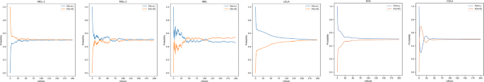

  

  The training results of the agent systems in the Pennies Matching game. The strategy probability parameters of actions L and R are approximated by the frequency. The game has a unique mixed Nash equilibrium P(A = L) = P(A = R) = 0.5. We can assume that the system converges to this equilibrium when the strategy parameters converge to 0.5

  When both x and y are positive integers, increasing the value of their sum leads to a decrease in the reward. Thus, x = y = 0 is the optimal solution to the game. However, acting greedily or “arrogantly” shaping the action of the opponent can lead to worse results.

We use this game environment to test the robustness of the algorithm in the opponent shaping process. Figure 4 shows the training results in the Tandem game. The MOL algorithm does not lead both agents to act “arrogantly”, but eventually converges to an optimal result. It achieves the same result as SOS and COLA without using the opponent’s real strategy information.

• (e) Stag Hunt game (with multiple agent) [24]: For multiagent systems, when the number of agents exceeds two, it leads to a significant increase in the state space and more complex equilibrium. Therefore, previous articles rarely include experiments with three or more agents. We refer to the classic Stag Hunt game (given in Table 6) and extend it to three agents:

  $$ \begin{aligned} & R^{i}(\text{Stag})= \begin{cases}4 & \text { if } a^{-i} = \text{Stag,} \ \forall a^{-i} \\ -10 & \text { else } \end{cases} \\ & R^{i}(\text{Hare})= \begin{cases}1 \quad & \text { if } a^{-i} = \text{Hare,} \ \forall a^{-i} \\ 3 \quad & \text { else } \end{cases} \end{aligned} $$

  (35)

  where i ∈{1,2,3}. The previous algorithms were only tested in the two-player Stag Hunt, and we applied MOL to a multiagent scenario for comparison. The results are shown in Fig. 5. It can be seen that MOL is also effective in multiagent scenarios.

Fig. 4

The training results of the agent systems in the Tandem game. The line with a joint reward of 0 corresponds to the optimal equilibrium x = y = 0

Table 6 Stag Hunt

Fig. 5

The training results of the agent systems in the Stag Hunt game using different algorithms. The line with a joint reward of 4 corresponds to the cooperation equilibrium, and the line with a joint reward of 1.0 corresponds to the local disadvantage result. The curve labeled MOL-2(MA) represents the application of MOL in multiagent Stag Hunt (with 3 players)

5.2 Randomly generated games

We examine the learning ability of an agent system with the MOL algorithm in randomly generated games. We generate 2,000 bimatrix games, with the reward corresponding to each of their joint actions being chosen from a determined set of integers. We allow agent systems with different algorithms to be trained in these environments and record their convergence results. Agents in this environment do not have access to information about other agents or their strategies. Therefore, avoiding a local inferior Nash equilibrium is the main objective. We use the Nash equilibrium with the highest average reward as the theoretical optimal result.

Figure 6 shows the joint score for different algorithms in randomly generated games. From the figure, we can see that the joint score of MOL is higher and is close to the optimal Nash equilibrium. This indicates that as a learning agent system MOL is more efficient and robust.

Fig. 6

Results of agent systems with different algorithms trained in 2,000 random game environments. The line labeled best_ne represents the average reward for the optimal Nash equilibrium in these games. The joint score is obtained by averaging the rewards for the last episode

We also record the performance of the algorithm in response to different Nash equilibrium environments in Table 7. $\bar {r}$ is the joint score for the algorithm, r(NE) is the joint reward for the optimal Nash equilibrium and k is a parameter. Therefore, k = 0.9 in PE means that the joint score of the algorithm is higher than 0.9 times the score of the optimal pure strategy equilibrium. We find that MOL achieves good results in exploring equilibrium that approach or exceed the optimal Nash equilibrium reward. Training pure strategies in game environments where only mixed equilibrium exist does not cause a significant decrease in the joint scores. Our algorithm achieves training results close to the optimal Nash equilibrium in the general case.

Table 7 The frequency of the convergence result that the algorithm scores above the optimal pure strategy equilibrium (PE) and mixed equilibrium (ME) in randomly generated games

5.3 Competitive environments

Since we cannot require agents to use the same learning method in a repeated game environment, the ability to cope with different opponents is also important. We therefore also conduct an experiment for evaluating the algorithm performance against different opponents. The environment used is the same generated bimatrix game, but random agents are used for training in each game. In this environment the agents do not have access to the (learning) strategy that the opponent will adopt and can only observe joint actions after each round of the game. Algorithms based on the private information of the opponent or on consistency (SOS, COLA) cannot be applied in this scenario. There are 20,000 randomly generated games, each with two selected agents (which may or may not use the same algorithm), that are added to the training over 100 episodes. We evaluate the performance of the algorithm from two perspectives. The first is the average score (the results are shown in Fig. 7) of the evolution process for agents with different algorithms over 100 episodes (obtained by training in 20,000 matrix games). This reflects the ability of the agents to adapt when faced with a diverse set of opponents. From Fig. 7, we can see that our algorithm achieves higher scores against diversified opponents.

Fig. 7

The training results for agents with different opponents. The curves represent the scores of the strategies learned by different algorithms within 100 episodes when facing a random opponent (averaged over 20,000 matrix games)

We also record the training results of each particular combination of agents in randomly generated games. Since the structure of the game is symmetric and randomized, agents who perform better have stronger applicability in noncooperative game environments. The experimental results are presented in Fig. 8. From Fig. 8, we find that MOL-2 does not receive a higher reward in a competitive game environment when facing LOLA or MOL-1, two algorithms that aim for short-term rewards. However, MOL-2 generally receives higher rewards against a variety of opponents (and simultaneously makes the opponents’ rewards higher). We can see that MOL performs well in striking a balance between increasing its own rewards and maximizing social welfare (the average reward for the agent system).

Fig. 8

Training results against different opponents. The row labels indicate the algorithm used by the agent, and the column labels indicate the algorithm used by the opponent. The values in the corresponding cells indicates the score of that agent against this class of opponents. A cell with a lighter color indicates a higher score

From the experiments above, we can see that MOL achieves good results in terms of improving the agent reward as well as social welfare. In the cooperative form of the game, MOL can converge to an equilibrium with higher joint rewards and effectively face different kinds of opponents in competitive environments. Since MOL is based on the best response (a pure strategy in most cases), the stability of MOL is reduced in game environments where only mixed equilibrium exists. However, we can see from the experimental results that this does not affect the final convergence results. Therefore MOL is more suitable for application in the repeated game environment of multiagent learning system, and as a baseline for opponent modeling due to its prosociality as well as its generalization capability.

6 Conclusion

This article proposes an MOL method for multiagent repeated game environments. By modeling the stable points of the opponent learning process and taking actions to guide the opponent, MOL can achieve a solution with a high reward equilibrium. Since there is no restriction on the opponent’s model during training and no private information of the other agents is used, MOL is more feasible for noncooperative game environments than other algorithms. We provide a proof of the convergence of MOL by dividing the algorithm into two looping phases and using the Nash equilibrium as a boundary constraint. MOL achieves good results in the classical game structure as well as in the randomly generated games, and obtains a higher joint score when dealing with different opponents. Additionally, we discuss the definition of the equilibrium concept in repeated games with learning processes. We argue that there are better convergence results that can be used as optimization objectives for multiagent systems and establish the relationship between our algorithm and Pareto optimality. We hope to provide a reference for the design of optimization objectives in the learning processes of agent systems, and to help build a general model for noncooperative game environments.

References

Fudenberg D, Levine DK (1998) The theory of learning in games. vol 1. MIT Press Books
Milgrom P, Roberts J (1991) Adaptive and sophisticated learning in normal form games. Games Econom Behav 3(1):82–100
Milgrom P, Roberts J (1990) Rationalizability, learning, and equilibrium in games with strategic complementarities. Econometrica 58(6):1255–1277
Dekel E, Fudenberg D, Levine D (1999) Payoff information and self-confirming equilibrium. J Econ Theory 89(2):165–185
Fudenberg D, Levine D (1993) Self-confirming equilibrium. Econometrica 61(3):523–545
Binmore K, Samuelson L (1999) Evolutionary drift and equilibrium selection. Rev Econ Stud 66(2):363–393
Du W, Ding S (2021) A survey on multi-agent deep reinforcement learning: from the perspective of challenges and applications. Artif Intell Rev 54(5):3215–3238
Gupta JK, Egorov M, Kochenderfer M (2017) Cooperative multi-agent control using deep reinforcement learning. In: International conference on autonomous agents and multiagent systems. Springer, Cham, pp 66–83
Jiang J, Lu Z (2018) Learning attentional communication for multi-agent cooperation. In: Advances in neural information processing systems 31, pp 7265–7275
Ge H, Ge Z, Sun L, et al. (2022) Enhancing cooperation by cognition differences and consistent representation in multi-agent reinforcement learning. Applied Intelligence
Deng C, Wen C, Wang W, et al. (2022) Distributed adaptive tracking control for high-order nonlinear multi-agent systems over event-triggered communication. IEEE Transactions on Automatic Control
Sunehag P, Lever G, Gruslys A, Czarnecki W, Zambaldi V, Jaderberg M, Lanctot M, Sonnerat N, Leibo J, Tuyls K, Graepe T (2017) Value-decomposition networks for cooperative multi-agent learning based on team reward. In: Proceedings of the 17th international conference on autonomous agents and multiagent systems
Rashid T, Samvelyan M, Witt CD, Farquhar G, Foerster J, Whiteson S (2018) QMIX: monotonic value function factorisation for deep multi-agent reinforcement learning. In: Proceedings of the 35th international conference on machine learning, pp 4295–4304
Rashid T, Farquhar G, Peng B, et al. (2020) Weighted qmix: expanding monotonic value function factorisation for deep multi-agent reinforcement learning. Adv Neural Inform Process Syst 33:10199–10210
Rashid T, Samvelyan M, De Witt CS, et al. (2020) Monotonic value function factorisation for deep multi-agent reinforcement learning. J Mach Learn Res 21(1):7234–7284
Kraemer L, Banerjee B (2016) Multi-agent reinforcement learning as a rehearsal for decentralized planning. Neurocomputing 190:82–94
Silver D, Hubert T, Schrittwieser J, et al. (2018) A general reinforcement learning algorithm that masters chess, shogi, and Go through self-play. Science 362(6419):1140–1144
Brown N, Kroer C, Sandholm T (2017) Dynamic thresholding and pruning for regret minimization. In: Proceedings of the AAAI conference on artificial intelligence, vol 31(1)
Brown N, Sandholm T (2018) Superhuman AI for heads-up no-limit poker Libratus beats top professionals. Science 359(6374):418–424
Jiang Q, Li K, Du B, Chen H, Fang H (2019) DeltaDou: expert-level Doudizhu AI through self-play. In: Proceedings of the twenty-eighth international joint conference on artificial intelligence, pp 1265–1271
Zha D, Xie J, Ma W, Zhang S, Lian X, Hu X, Liu J (2021) DouZero: mastering DouDizhu with self-play deep reinforcement learning. In: Proceedings of the 38th international conference on machine learning, vol 139, pp 12333–12344
Abdallah S, Kaisers M (2016) Addressing environment non-stationarity by repeating Q-learning updates. J Mach Learn Res 17(1):1582–1612
Tang Z, Yu C, Chen B, Xu H, Wang X, Fang F, Du S, Wang Y, Wu Y (2021) Discovering diverse multi-agent strategic behavior via reward randomization. In: International conference on learning representations, pp 1–26
He H, Boyd-Graber J, Kwok K, Daume H (2016) Opponent modeling in deep reinforcement learning. In: Proceedings of the 33rd international conference on machine learning, pp 1804–1813
Foerster J, Chen R, Al-Shedivat M, Whiteson S, Abbeel P, Mordatch I (2018) Learning with opponent-learning awareness. In: Proceedings of the 17th international conference on autonomous agents and multiagent systems, pp 122–130
Schäfer F, Anandkumar A (2019) Competitive gradient descent. Adv Neural Inf Process Syst, 32
Willi T, Letcher A, Treutlein J, et al. (2022) COLA: consistent learning with opponent-learning awareness. In: International conference on machine learning. PMLR, pp 23804–23831
Damme EV, Hurkens S (1999) Endogenous Stackelberg leadership. Games Econ Behav 28 (1):105–129
Liu H, Wang X, Zhang W, et al. (2020) Infrared head pose estimation with multi-scales feature fusion on the IRHP database for human attention recognition. Neurocomputing 411:510–520
Liu T, Liu H, Li YF, et al. (2019) Flexible FTIR spectral imaging enhancement for industrial robot infrared vision sensing. IEEE Trans Industr Inform 16(1):544–554
Liu H, Nie H, Zhang Z, et al. (2021) Anisotropic angle distribution learning for head pose estimation and attention understanding in human-computer interaction. Neurocomputing 433:310–322
Bowling M, Veloso M (2001) Rational and convergent learning in stochastic games. In: Proceedings of seventeenth international joint conference on artificial intelligence, pp 1021–1026
Conitzer V, Sandholm T (2003) AWESOME: a general multiagent learning algorithm that converges in self-play and learns a best response against stationary opponents. Mach Learn 67(1):23–43
Osband I, Blundell C, Pritzel A, et al. (2016) Deep exploration via bootstrapped DQN. Advances in Neural Information Processing Systems, 9
Liu H, Liu T, Zhang Z, et al. (2022) ARHPE: asymmetric relation-aware representation learning for head pose estimation in industrial human-machine interaction. IEEE Trans Industr Inform 18:7107–7117
Liu H, Zheng C, Li D, et al. (2021) EDMF: efficient deep matrix factorization with review feature learning for industrial recommender system. IEEE Trans Industr Inform 18(7):4361–4371
Aotani T, Kobayashi T, Sugimoto K (2021) Bottom-up multi-agent reinforcement learning by reward shaping for cooperative-competitive tasks. Appl Intell 51:4434–4452
Letcher A, Foerster J, Balduzzi D, Rocktaschel T, Whiteson S (2019) Stable opponent shaping in differentiable games. In: International conference on learning representations, pp 1–20
Zhang C, Lesser V (2010) Multi-agent learning with policy prediction. In: Proceedings of the twenty-fourth AAAI conference on artificial intelligence, pp 927–934
Wen Y, Chen H, Yang Y, Tian Z, Li M, Chen X, Wang J (2021) Multi-agent trust region learning. In: Proceedings of the seventh international conference on learning representations, pp 1–20
Kim DK, Liu M, Riemer MD, et al. (2021) A policy gradient algorithm for learning to learn in multiagent reinforcement learning. In: International conference on machine learning PMLR, pp 5541–5550
Raileanu R, Denton E, Szlam A, Fergus R (2018) Modeling others using oneself in multi-agent reinforcement learning. In: Proceedings of the 35th international conference on machine learning, pp 4257–4266
Zhen Z, Yew-Soon D, Xue B (2019) Wang a collaborative multiagent reinforcement learning method based on policy gradient potential. IEEE Trans Cybern 51(2):1015–1027
Hu Y, Gao Y, An B (2015) Multiagent reinforcement learning with unshared value functions. IEEE Trans Cybern 45(4):647– 662
Athey S (2001) Single crossing properties and the existence of pure strategy equilibria in games of incomplete information. Econometrica 69(4):861–889
Marris L, Muller P, Lanctot M, Tuyls K, Graepel T (2021) Multi-agent training beyond zero-sum with correlated equilibrium meta-solvers. In: Proceedings of the 38th international conference on machine learning, vol 139, pp 7480–7491
Wang B, Zhang Y, Zhou ZH, et al. (2019) On repeated stackelberg security game with the cooperative human behavior model for wildlife protection. Appl Intell 49:1002–1015
Auer P, Cesa-Bianchi N, Fischer P (2002) Finite-time analysis of the multiarmed bandit problem. Mach Learn 47(2):235– 256
Harsanyi J (1973) Games with randomly disturbed payoffs: a new rationale for mixed-strategy equilibrium points. Int J Game Theory 2:1–23
Acknowledgements
This paper is supported by National Key R&D Program of China (2021YFA1000403) and National Natural Science Foundation of China (No.11991022), and the Strategic Priority Research Program of Chinese Academy of Sciences, Grant No.XDA27000000.
Author information
Authors and Affiliations
Corresponding author
Additional information
Publisher’s note
Springer Nature remains neutral with regard to jurisdictional claims in published maps and institutional affiliations.
Rights and permissions
Open Access This article is licensed under a Creative Commons Attribution 4.0 International License, which permits use, sharing, adaptation, distribution and reproduction in any medium or format, as long as you give appropriate credit to the original author(s) and the source, provide a link to the Creative Commons licence, and indicate if changes were made. The images or other third party material in this article are included in the article's Creative Commons licence, unless indicated otherwise in a credit line to the material. If material is not included in the article's Creative Commons licence and your intended use is not permitted by statutory regulation or exceeds the permitted use, you will need to obtain permission directly from the copyright holder. To view a copy of this licence, visit http://creativecommons.org/licenses/by/4.0/.
About this article
Cite this article
Hu, Y., Han, C., Li, H. et al. Modeling opponent learning in multiagent repeated games. Appl Intell 53, 17194–17210 (2023). https://doi.org/10.1007/s10489-022-04249-x
Accepted:
Published:
Issue Date:
DOI: https://doi.org/10.1007/s10489-022-04249-x