Entropy-Transport distances between unbalanced metric measure spaces

Abstract

Inspired by the recent theory of Entropy-Transport problems and by the ${\mathbf {D}}$-distance of Sturm on normalised metric measure spaces, we define a new class of complete and separable distances between metric measure spaces of possibly different total mass. We provide several explicit examples of such distances, where a prominent role is played by a geodesic metric based on the Hellinger-Kantorovich distance. Moreover, we discuss some limiting cases of the theory, recovering the “pure transport” ${\mathbf {D}}$-distance and introducing a new class of “pure entropic” distances. We also study in detail the topology induced by such Entropy-Transport metrics, showing some compactness and stability results for metric measure spaces satisfying Ricci curvature lower bounds in a synthetic sense.

1 Introduction

With motivations from pure Mathematics as well as from applied sciences, over the last decades a growing attention has been paid to the problem of “comparing objects”, which come naturally endowed with a distance/metric and a weight/volume form/measure. From the mathematical point of view, such objects are formalised as metric measure spaces (m.m.s. for short) $(X,{\mathsf {d}},\mu )$, where the metric structure $(X,{\mathsf {d}})$ describes the geometry and the mutual distance of points, and the measure $\mu$ “weights” the relative importance of different parts of the object.

The flexibility of such a framework allows to unify the treatment of a series of problems stemming from various fields of science and technology, e.g. chemistry [24], data science [33], multi-omics data alignment [13], computer vision [40], language processing [1], graph [46] and shape [42, 49] matching, barycenters & shape analysis [34], generative networks [6, 11], machine learning [47]. The theory of metric measure spaces has been flourishing in pure Mathematics as well, providing a unified setting to investigate concentration of measure phenomena [26, 41], the theory of Ricci limit spaces [8, 19] and, more generally, synthetic notions of Ricci curvature lower bounds [4, 30, 43, 44].

In order to “quantify the similarities and differences between two such objects”, it is thus natural to investigate appropriate notions of distance between metric measure spaces. This idea has its roots in the work of Gromov [23,  Chapter 3$\frac{1}{2}$]), who first recognized the importance of studying the “space of spaces” $\varvec{\mathrm {X}}$ as a metric space in its own right. Formally, $\varvec{\mathrm {X}}$ denotes the set of equivalence classes of metric measure spaces $(X,{\mathsf {d}},\mu )$, where $(X,{\mathsf {d}})$ is a complete and separable metric space, and $\mu$ is a finite, nonnegative, Borel measure; we are naturally identifying two m.m.s. $(X_1,{\mathsf {d}}_1,\mu _1)$, $(X_2,{\mathsf {d}}_2,\mu _2)$ if there exists an isometry $\psi :{\mathsf {supp}}(\mu _1)\rightarrow {\mathsf {supp}}(\mu _2)$ such that $\psi _{\sharp }\,\mu _1=\mu _2$. Here by ${\mathsf {supp}}(\mu )$ we denote the support of the measure $\mu$ (see the preliminary section for more details).

In the recent years, the theory has been pushed forward by the works of Sturm [43, 45] and Memoli [32] who realized that ideas from mass transportation can be used to produce new relevant distances between metric measure spaces. Such distances have been successfully applied in different fields, but suffer from a major restriction which is intrinsic of the Wasserstein distances coming from optimal transport: they can be used to compare only spaces with the same total mass.

The goal of the present paper is to overcome this limitation by taking advantage of the theory of optimal Entropy-Transport problems [29]. In contrast with the classical transport setting, these problems allow the description of phenomena where the conservation of mass may not hold; for this reason they are also known in the literature as “unbalanced optimal transport problems”. The corresponding theory is fairly recent and is becoming increasingly popular in applications, e.g. gradient flows to train neural networks [9, 37], supervised learning [18], medical imaging [17] and video [27] registration. Indeed, the Entropy-Transport relaxation seems to outperform classical optimal transport in all the problems where the input data is noisy or a normalization procedure is not appropriate. We refer to [38] and references therein for more applications of unbalanced optimal transport.

As we are going to explain in detail below, inspired by the construction of the ${\mathbf {D}}$-distance of Sturm [43], we are able to produce a new class of complete and separable distances between metric measure spaces by replacing the Wasserstein distance with an Entropy-Transport distance. Such metric structures on $\varvec{\mathrm {X}}$ also turn out to be geodesic (resp. length) when the underlying Entropy-Transport distance is geodesic (resp. length).

Optimal transport and Sturm distances. Let $(X,{\mathsf {d}})$ be a metric space and $\varvec{\mathrm c}:X\times X\rightarrow [0,+\infty ]$ be a lower semi-continuous cost function. The optimal transport problem between two probability measures $\mu _1,\mu _2$ consists in the minimization problem:

$$\begin{aligned} \mathrm {T}(\mu _1,\mu _2):=\inf _{\varvec{\gamma }\in \Pi (\mu _1,\mu _2)}\int _{X\times X}\varvec{\mathrm c}(x_1,x_2)\, {\mathrm d}\varvec{\gamma }(x_1,x_2). \end{aligned}$$

(1)

Here $\Pi (\mu _1,\mu _2)$ denotes the set of measures $\varvec{\gamma }$ in the product space $X\times X$ whose marginals satisfy the constraint $\pi ^i_{\sharp }\varvec{\gamma }=\mu _i$, where $\pi ^i$ denotes the projection map $\pi ^i(x_1,x_2)=x_i$.

A typical choice for the cost function is $\varvec{\mathrm c}(x_1,x_2)={\mathsf {d}}^p(x_1,x_2)$, $p\ge 1$. In this situation, the transport cost $\mathrm {T}$ is the p-power of the celebrated p-Wasserstein distance ${\mathcal {W}}_p$, a metric on the set ${\mathscr {P}}_p(X)$ of probability measures over X with finite p-moment. Starting from the seminal work of Kantorovich, the metric space $({\mathscr {P}}_p(X), {\mathcal {W}}_p)$ has been thoroughly studied: it inherits many geometric properties of the underlying space $(X,{\mathsf {d}})$ (such as completeness, separability, geodesic property) and induces the weak topology (with p-moments) of probability measures. We refer to the monograph [48] for a detailed overview of the topic.

As observed by Sturm [43], one can lift the metric ${\mathcal {W}}_p$ to a distance between metric measure spaces by defining:

$$\begin{aligned} {\mathbf {D}}_p\left( (X_1,{\mathsf {d}}_1,\mu _1),(X_2,{\mathsf {d}}_2,\mu _2)\right) :=\inf {\mathcal {W}}_p(\psi ^1_{\sharp }\mu _1,\psi ^2_{\sharp }\mu _2), \end{aligned}$$

(2)

where the infimum is taken over all complete and separable metric spaces $({\hat{X}},\hat{{\mathsf {d}}})$, and all isometric embeddings $\psi ^i:{\mathsf {supp}}(\mu _i)\rightarrow {\hat{X}}$. It is proved in [43,  Theorem 3.6] that ${\mathbf {D}}_p$ is a complete, separable and geodesic distance on the set

$$\begin{aligned} \varvec{\mathrm {X}}_{1,p}:=\{ (X,{\mathsf {d}},\mu )\in \varvec{\mathrm {X}}: \ \mu \in {\mathscr {P}}_p(X,{\mathsf {d}})\}. \end{aligned}$$

Entropy-Transport problems and Sturm-Entropy-Transport distances. The idea at the core of Entropy-Transport problems is to relax the marginal constraints typical of the classical Kantorovich formulation (1) by adding some suitable penalizing functionals which keep track of the deviation of the marginals $\gamma _i:=\pi ^i_{\sharp }\varvec{\gamma }$ from the data $\mu _i$, $i=1,2$.

Following the approach of Liero, Mielke and Savaré [29], given a superlinear, convex function $F:[0,+\infty )\rightarrow [0,+\infty ]$ such that $F(1)=0$ (for simplicity here we assume F to be superlinear, see definition (21) for the general case), one considers the entropy functional (also called Csiszár F-divergence [12])

$$\begin{aligned} D_F:{\mathscr {M}}(X)\times {\mathscr {M}}(X)\rightarrow [0,+\infty ], \quad D_F(\gamma ||\mu ):={\left\{ \begin{array}{ll} \int _X F\left( \frac{\mathrm {d}\gamma }{\mathrm {d}\mu }\right) \mathrm {d} \mu \quad &{}\text {if} \ \gamma \ll \mu , \\ +\infty &{}\text {otherwise}. \end{array}\right. }\nonumber \\ \end{aligned}$$

(3)

Here ${\mathscr {M}}(X)$ denotes the set of finite, nonnegative, Borel measures over X. A classical example is given by the choice $F=U_1(s):=s\ln (s)-s+1$, that corresponds to the celebrated Kullback-Leibler divergence (note that when ${\varvec{\gamma }}$ and $\mu$ are probability measures, $D_{U_1}$ coincides with the celebrated Boltzmann-Shannon entropy $\mathrm{Ent}(\rho \mu | \mu )=\int \rho \log \rho \, {\mathrm d}\mu$).

Given $\mu _1,\mu _2\in {\mathscr {M}}(X)$, the Entropy-Transport problem induced by the entropy function F and the cost function $\varvec{\mathrm c}$ is then defined as

(4)

We emphasize that the problem (4) makes perfect sense even when $\mu _1(X)\ne \mu _2(X)$.

As in the case of optimal transport problems, it is natural to consider cost functions of the form $\varvec{\mathrm c}(x_1,x_2)=\ell ({\mathsf {d}}(x_1,x_2))$, where ${\mathsf {d}}$ is a distance on X and $\ell :=[0,\infty )\rightarrow [0,\infty ]$ is a general function. With a careful choice of the functions F and $\ell$ (see [14] for a discussion on the metric properties of Entropy-Transport problems), one is able to produce a distance on the space ${\mathscr {M}}(X)$ by taking a suitable power of the Entropy-Transport cost , namely for a certain $a\in (0,1]$.

In the paper we introduce the class of regular Entropy-Transport distances. The formal definition of this class of distances is given in Definition 2, here we just mention than any regular Entropy-Transport distance is a complete and separable metric on ${\mathscr {M}}(X)$ of the form , for an Entropy-Transport cost induced by sufficiently regular functions F and $\ell$.

For any regular Entropy-Transport distance, the Sturm-Entropy-Transport distance between the (equivalence classes of) m.m.s. $(X_1,{\mathsf {d}}_1,\mu _1)$, $(X_2,{\mathsf {d}}_2,\mu _2)$ is then defined as

(5)

where the infimum is taken over all complete and separable metric spaces $({\hat{X}},\hat{{\mathsf {d}}})$, and all isometric embeddings $\psi ^1:{\mathsf {supp}}(\mu _1)\rightarrow {\hat{X}}$ and $\psi ^2:{\mathsf {supp}}(\mu _2)\rightarrow {\hat{X}}$.

The main result of the paper (Theorem 2) is that every Sturm-Entropy-Transport distance defines a complete and separable metric structure on ${\mathbf {X}}$. Moreover it satisfies the geodesic (resp. length) property if the distance satisfies the geodesic (resp. length) property on the space of measures.

We also study in detail the notion of convergence induced by such distances, showing that it corresponds to the weak measured-Gromov convergence introduced in [21]. As a consequence, we obtain a compactness result for the class of m.m.s. $(X,{\mathsf {d}},\mu )$ satisfying the ${\mathsf {CD}}(K,N)$ condition, having bounded diameter and satisfying $0<v\le \mu (X)\le V$. We refer to Theorem 4 for the precise statement and to the preliminaries for the definition of the curvature-dimension condition ${\mathsf {CD}}(K,N)$.

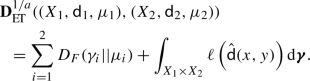
At a technical level, the proofs of our results are inspired by the corresponding ones given by Sturm in [43], but they require new ideas in order to deal with general cost functions and with the entropic part of the problem. Two key results of independent interest are contained in Proposition 2 and Lemma 6, where we show that the infimum in the right hand side of (5) is actually a minimum, and we give an explicit formulation of the Sturm-Entropy-Transport distance, namely

(6)

for some optimal measure $\varvec{\gamma }\in {\mathscr {M}}(X_1\times X_2)$ and optimal pseudo-metric coupling $\hat{{\mathsf {d}}}$ between ${\mathsf {d}}_1$ and ${\mathsf {d}}_2$ (see the preliminaries for the definition of pseudo-metric coupling). Also the proof of one of the main results, Theorem 2, despite being inspired by [43], departs from it and needs some new ideas:

• in order to show that ${\mathbf {D}}_p$ defines a non-degenerate distance function (i.e.

  $$\begin{aligned} {\mathbf {D}}_p \left( (X_1,{\mathsf {d}}_1,\mu _1), (X_2,{\mathsf {d}}_2,\mu _2) \right) =0 \end{aligned}$$

  implies that $(X_1,{\mathsf {d}}_1,\mu _1)$ and $(X_2,{\mathsf {d}}_2,\mu _2)$ are isomorphic as metric measure spaces), Sturm [43] establishes a comparison result with Gromov’s ${\underline{\Box }}_{1}$ distance, of independent interest; this permits to inherit the non-degeneracy of ${\mathbf {D}}_p$ by the one of ${\underline{\Box }}_{1}$.

  Instead, we argue directly: thanks to the aforementioned Proposition 2 and Lemma 6, we can exploit the existence of an optimal coupling both at the level of space and measure and infer the non-degeneracy of directly;

• in order to show that the ${\mathbf {D}}_p$ distance is length, Sturm [43] argues by approximation via finite metric spaces, taking advantage of the “pure transport” behaviour of ${\mathbf {D}}_p$.

  Due to the entropy contribution in the distance, we argue differently: the main point is to embed everything in a complete, separable and geodesic ambient space, obtained by a slight modification of Kuratowski embedding.

The class of regular Entropy-Transport distances includes some of the main examples of Entropy-Transport distances known in the literature, including:

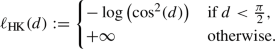
• The Hellinger-Kantorovich geodesic distance [10, 25, 28, 29] induced by the choices

  $$\begin{aligned} a=1/2\, , \qquad F(s)=U_1(s)\, , \qquad \ell (d)={\left\{ \begin{array}{ll} -\log \left( {\cos ^2(d)}\right) \ \ &{}\text {if} \ d<\frac{\pi }{2}, \\ +\infty \ \ &{}\text {otherwise}.\end{array}\right. } \end{aligned}$$

• The so-called Gaussian Hellinger-Kantorovich distance [29] that corresponds to the choices

  $$\begin{aligned} a=1/2\, , \qquad F(s)=U_1(s)\, , \qquad \ell (d)=d^2. \end{aligned}$$

• The quadratic power-like distances studied in [14] corresponding to

  $$\begin{aligned} a=1/2\, , \quad F(s)=U_p(s):=\frac{s^p-p(s-1)-1}{p(p-1)}\, , \quad \ell (d)=d^2, \quad 1<p\le 3. \end{aligned}$$

Moreover, our analysis is not restricted to regular Entropy-Transport distances. By a limit procedure we also discuss some singular cases covering:

• The “pure entropy” setting that corresponds to the choice

  $$\begin{aligned} \varvec{\mathrm c}(x_1,x_2)={\left\{ \begin{array}{ll}0 \ &{}\text {if} \ x_1=x_2, \\ +\infty &{}\text {otherwise.} \end{array}\right. } \end{aligned}$$

  In this situation we construct a family of distances between metric measure spaces inducing a notion of strong convergence (see Theorems 5 and 6 for the details).

• The “pure transport” setting, corresponding to

  $$\begin{aligned} a=1/p\, , \qquad F(s)={\left\{ \begin{array}{ll} 0 \ &{}\mathrm {if} \ s=1, \\ +\infty &{}\mathrm {otherwise}, \end{array}\right. } \qquad \ell (d)=d^p, \end{aligned}$$

  where we recover the ${\mathbf {D}}_p$-distances introduced by Sturm.

• The Piccoli-Rossi distance $\mathsf {BL}$ [35, 36] (also known as bounded-Lipschitz distance), induced by the choices

  $$\begin{aligned} a=1\, , \qquad F(s)=|s-1|\, , \qquad \ell (d)=d. \end{aligned}$$

  By an analogous procedure to the one described in (5), in Theorem 8 we show that the distance $\mathsf {BL}$ can be lifted to a complete distance ${\mathbf {BL}}$ on the set ${\mathbf {X}}$.

Note on the preparation. Some of the results of the paper (often under additional assumptions) have been presented at different seminars and included in the Phd thesis of the first named author [15,  Chapter 5], where the construction of the Sturm-Entropy-Transport distances induced by the Hellinger-Kantorovich and the quadratic power-like distances is developed.

Only during the final stage of preparation of the present manuscript (September 2020), we became aware of the independent work [39], which defines a class of distances (denoted by $\mathrm {CGW}$, for “conic Gromow-Wasserstein”) between unbalanced metric measure spaces starting from the construction of the Gromov–Wasserstein distance introduced in [32] and the conical formulation of the Entropy-Transport problems (see [10, 14, 29] and Remark 1 for a discussion on the “cone geometry” of Entropy-Transport problems). The paper [39] also provides some interesting numerical discussions on the topic, while it is not present a study on the analytic and geometric properties of this class of distances (such as completeness, separability, the length and geodesic property, compactness). An expert reader will notice that our distance is an unbalanced counterpart of Sturm’s ${\mathbf {D}}_p$ distance [43] for probability metric measure spaces, while Séjourné-Vialard-Peyré $\mathrm {CGW}$ distance [39] is an unbalanced counterpart of Memoli’s [32] Gromov–Wasserstein distance. A major difference between the two approaches is that while our distance is complete (see Theorem 2), the Gromov–Wasserstein distance of [32] is not complete, and the same is expected for the $\mathrm {CGW}$ distance of [39]. The relation between and $\mathrm {CGW}$ is analysed in Sect. 5, where we prove an upper bound of the latter in terms of the former.

2 Preliminaries and notation

2.1 Metric and measure setting

A function ${\mathsf {d}}:X\times X\rightarrow [0,\infty ]$ is a pseudo-metric on the set X if ${\mathsf {d}}$ is symmetric, satisfies the triangle inequality and ${\mathsf {d}}(x,x)=0$ for every $x\in X$. We say that ${\mathsf {d}}$ is a metric possibly attaining the value $+\infty$ if it is a pseudo-metric such that ${\mathsf {d}}(x,y)=0$ implies $x=y$. When ${\mathsf {d}}$ is also finite-valued, we simply say that ${\mathsf {d}}$ is a metric. A pseudo-metric space (resp. metric space) will be a couple $(X,{\mathsf {d}})$, where ${\mathsf {d}}$ is a pseudo-metric (resp. metric) on the set X.

On a pseudo-metric space we will always consider the topology induced by the open balls $B_r(x):=\{y\in X: {\mathsf {d}}(x,y)<r\}.$ A Polish space is a separable completely metrizable topological space. We will denote by $\mathsf {diam}(X)$ the diameter of a metric space X.

An isometry between two metric spaces $(X_1,{\mathsf {d}}_1)$, $(X_2,{\mathsf {d}}_2)$ is a map $\psi :X_1\rightarrow X_2$ such that for every $x,y\in X_1$ we have

$$\begin{aligned} {\mathsf {d}}_1(x,y)={\mathsf {d}}_2(\psi (x),\psi (y)). \end{aligned}$$

(7)

Let $\{(X_{\alpha },{\mathsf {d}}_{\alpha })|{\alpha }\in A\}$ be an indexed family of metric spaces, we define its disjoint union as

$$\begin{aligned} \bigsqcup _{\alpha }X_{\alpha }:=\bigcup \left\{ X_{\alpha }\times \{\alpha \}|{\alpha }\in A\right\} , \end{aligned}$$

endowed with a pseudo-metric $\hat{{\mathsf {d}}}$, called pseudo-metric coupling between $\{{\mathsf {d}}_{\alpha }\}$, such that $\hat{{\mathsf {d}}}((x,\alpha ),(y,\alpha ))={\mathsf {d}}_{\alpha }(x,y)$ for every $x,y\in X_{\alpha }$. The inclusion map

$$\begin{aligned} \iota _{\alpha }:X_{\alpha }\rightarrow \bigsqcup _{\alpha }X_{\alpha }, \ \ \ \iota _{\alpha }(x):=(x,\alpha ), \end{aligned}$$

is thus an isometry with image $X_{\alpha }\times \{\alpha \}$. We will often identify, with a slight abuse of notation, the space $X_{\alpha }$ with $X_{\alpha }\times \{\alpha \}$.

Lemma 1

Let $(X_1,{\mathsf {d}}_1)$, $(X_2,{\mathsf {d}}_2)$ be two complete and separable metric spaces. Let ${\hat{{\mathsf {d}}}}$ be a finite valued pseudo-metric coupling between ${\mathsf {d}}_1$ and ${\mathsf {d}}_2$. Then the space

$$\begin{aligned} {\tilde{X}}:=(X_1\sqcup X_2)/\sim \qquad \textit{where} \qquad x_1\sim x_2 \Longleftrightarrow {\hat{{\mathsf {d}}}}(x_1,x_2)=0 \end{aligned}$$

(8)

endowed with the distance

$$\begin{aligned} {\tilde{{\mathsf {d}}}}([x_1],[x_2]):={\hat{{\mathsf {d}}}}(x_1,x_2) \end{aligned}$$

is a complete and separable metric space. Here $[x]\in {\tilde{X}}$ denotes the equivalence class of the point $x\in X_1\sqcup X_2$.

Proof

We firstly notice that ${\tilde{{\mathsf {d}}}}$ is well defined on ${\tilde{X}}$. Indeed, if $x_1 \sim {\tilde{x}}_1$ and $x_2 \sim {\tilde{x}}_2$ we have

$$\begin{aligned} \begin{aligned} {\tilde{{\mathsf {d}}}}(x_1,x_2)&={\hat{{\mathsf {d}}}}(x_1,x_2)\le {\hat{{\mathsf {d}}}}(x_1,{\tilde{x}}_1)+{\hat{{\mathsf {d}}}}({\tilde{x}}_1,{\tilde{x}}_2)+{\hat{{\mathsf {d}}}}({\tilde{x}}_2, x_2) ={\tilde{{\mathsf {d}}}}({\tilde{x}}_1,{\tilde{x}}_2)\\ {\tilde{{\mathsf {d}}}}({\tilde{x}}_1,{\tilde{x}}_2)&={\hat{{\mathsf {d}}}}({\tilde{x}}_1,{\tilde{x}}_2)\le {\hat{{\mathsf {d}}}}({\tilde{x}}_1, x_1)+{\hat{{\mathsf {d}}}}(x_1,x_2)+{\hat{{\mathsf {d}}}}(x_2,{\tilde{x}}_2)={\tilde{{\mathsf {d}}}}(x_1,x_2) \end{aligned} \end{aligned}$$

which implies ${\tilde{{\mathsf {d}}}}(x_1,x_2)={\tilde{{\mathsf {d}}}}({\tilde{x}}_1,{\tilde{x}}_2)$.

It is clear that ${\tilde{{\mathsf {d}}}}$ is a metric on $(X_1\sqcup X_2)/\sim$.

The separability is a consequence of the fact that $(X_1\sqcup X_2,{\hat{{\mathsf {d}}}})$ is separable, being the union of two separable space (recall that ${\hat{{\mathsf {d}}}}={\mathsf {d}}_i$ on $X_i$, $i=1,2$).

To prove the completeness, let us consider a Cauchy sequence $\{y_j\}\in {\tilde{X}}$. It is sufficient to show that a subsequence is converging with respect to ${\tilde{{\mathsf {d}}}}$. Let $p:X_1\sqcup X_2\rightarrow {\tilde{X}}$ be the quotient map and, recalling that $X_1\sqcup X_2=X_1\times \{0\}\cup X_2\times \{1\}$, we can suppose without loss of generality that there exists a subsequence $\{p^{-1}(y_{j_k})\}\in X_1\times \{0\}$ (the case $\{p^{-1}(y_{j_k})\}\in X_2\times \{1\}$ being analogous). Up to identifying $(X_1\times \{0\},{\hat{{\mathsf {d}}}})$ with $(X_1,{\mathsf {d}}_1)$, we can infer that $\{p^{-1}(y_{j_k})\}$ is a Cauchy sequence in the complete space $(X_1,{\mathsf {d}}_1)$ and thus it converges. It is immediate to check that $\{y_{j_k}\}$ is converging in ${\tilde{X}}$ with respect to ${\tilde{{\mathsf {d}}}}$ and the proof is complete. $\square$

Starting from a metric space $(X,{\mathsf {d}})$, we define the cone over X as the space

$$\begin{aligned}&{\mathfrak {C}}(X):=(X\times [0,+\infty ))/{\sim } \quad \text {where} \quad (x_1,r_1)\sim (x_2,r_2)\\&\quad \iff r_1=r_2=0 \ \text{ or } \ r_1=r_2, x_1=x_2. \end{aligned}$$

If $(X,{\mathsf {d}})$ is a pseudo-metric space, we denote by ${\mathscr {M}}(X)$ the space of finite, nonnegative measures on the Borel $\sigma$-algebra ${\mathscr {B}}(X)$, and by ${\mathscr {P}}(X)\subset {\mathscr {M}}(X)$ the space of probability measures. We endow ${\mathscr {M}}(X)$ with the weak topology, inducing the following notion of convergence:

$$\begin{aligned} \mu _n\rightharpoonup \mu \iff \int _X f{\mathrm d}\mu _n \rightarrow \int _X f{\mathrm d}\mu \ \ \text {for any} \ f\in C_b(X), \end{aligned}$$

(9)

where $C_b(X)$ denotes the set of real, continuous and bounded functions defined on X.

A subset ${\mathscr {K}}\subset {\mathscr {M}}(X)$ is bounded if $\sup _{\mu \in {\mathscr {K}}}\mu (X)<\infty$ and it is equally tight if

$$\begin{aligned} \forall \epsilon >0 \ \ \exists K_{\epsilon }\subset X \ \text {compact}: \ \forall \mu \in {\mathscr {K}}, \ \ \mu (X{\setminus } K_{\epsilon })\le \epsilon . \end{aligned}$$

(10)

Compactness properties with respect to the weak topology on ${\mathscr {M}}(X)$ are guaranteed by the following version of Prokhorov’s Theorem:

Theorem 1

Let X be a Polish space. A subset ${\mathscr {K}}\subset {\mathscr {M}}(X)$ is bounded and equally tight if and only if it is relatively compact with respect to the weak topology.

We recall that the set of measures of the form

$$\begin{aligned} \mu =M\sum _{n=1}^N \delta _{x_n}, \end{aligned}$$

(11)

where $M\in {\mathbb {R}}_+$, $N\in {\mathbb {N}}$ and $x_n\in X$, is dense in ${\mathscr {M}}(X)$. Moreover, if X is separable, the measures of the form (11), with $M\in {\mathbb {Q}}_+$ and $x_n$ in a countable dense subset of X, form a countable dense subset of ${\mathscr {M}}(X)$, proving that also the latter is a separable space.

A metric measure space will be a triple $(X,{\mathsf {d}},\mu )$ where $(X,{\mathsf {d}})$ is a complete, separable metric space and $\mu \in {\mathscr {M}}(X)$. If there exists a point $x_0\in X$ such that

$$\begin{aligned} \int _X {\mathsf {d}}^p(x_0,x){\mathrm d}\mu (x)<\infty , \end{aligned}$$

(12)

we will say that the measure $\mu \in {\mathscr {P}}(X)$ has finite p-moment. We denote by ${\mathscr {P}}_p(X)$ the space of measures $\nu \in {\mathscr {P}}(X)$ with finite p-moment.

The support of the measure $\mu$ is the smallest closed set $X_0:={\mathsf {supp}}(\mu )$ such that $\mu (X{\setminus } X_0)=0$. We notice that the set ${\mathsf {supp}}(\mu )$ has a natural structure of metric measure space with the induced distance, $\sigma$-algebra and measure (which will be denoted in the same way).

We say that $\varphi$ is a curve connecting $x,y\in X$, if $\varphi :[a,b]\rightarrow X$ is a continuous map such that $\varphi (a)=x$ and $\varphi (b)=y$. The length of a curve is defined as

$$\begin{aligned} \mathsf {Length}(\varphi ):=\sup \sum _{i=1}^n {\mathsf {d}}\left( \varphi (t_{i-1}),\varphi (t_i)\right) , \end{aligned}$$

(13)

where the supremum is taken over all the partitions $a=t_0<t_1<\ldots <t_n=b$.

We will always assume that a curve of finite length is parametrized by constant speed, i.e.

$$\begin{aligned} \mathsf {Length}(\varphi \restriction _{[s,t]})=\frac{t-s}{b-a}\mathsf {Length}(\varphi ). \end{aligned}$$

(14)

A metric space $(X,{\mathsf {d}})$ is called length space if for all $x,y\in X$

$$\begin{aligned} {\mathsf {d}}(x,y)=\inf \left\{ \mathsf {Length}(\varphi ):\varphi \ \text {curve connecting} \ x \ \text {and} \ y\right\} . \end{aligned}$$

(15)

A geodesic is a curve $\varphi :[a,b]\rightarrow X$ such that

$$\begin{aligned} {\mathsf {d}}(\varphi (a), \varphi (t))= \frac{t-a}{b-a}\, {\mathsf {d}}(\varphi (a), \varphi (b)), \quad \text {for all } t\in [a,b] . \end{aligned}$$

Notice in particular that if $\varphi$ is a geodesic then

$$\begin{aligned} \mathsf {Length}(\varphi )={\mathsf {d}}(\varphi (a),\varphi (b)). \end{aligned}$$

A metric space $(X,{\mathsf {d}})$ is geodesic if any pair of points $x,y\in X$ is connected by a geodesic.

For a metric space $(X,{\mathsf {d}})$, the Kantorovich-Wasserstein distance ${\mathcal {W}}_p$ of order p, $p\ge 1$, is defined as follows: for $\mu _0,\mu _1 \in {\mathscr {M}}(X)$ we set

$$\begin{aligned} {\mathcal {W}}^p_p(\mu _0,\mu _1) := \inf _{\varvec{\gamma }} \int _{X\times X} {\mathsf {d}}^p(x,y) \, {\mathrm d}\varvec{\gamma }, \end{aligned}$$

(16)

where the infimum is taken over all $\varvec{\gamma } \in {\mathscr {M}}(X \times X)$ with $\mu _0$ and $\mu _1$ as the first and the second marginal, i.e. $(\pi ^i)_{\sharp }\varvec{\gamma }=\mu _i$ where $\pi ^i:X\times X\rightarrow X$ denotes the projection map $\pi ^i(x_1,x_2)=x_i$, $i=1,2$. A measure $\varvec{\gamma } \in {\mathscr {M}}(X \times X)$ achieving the minimum in (16) with given marginals is said a ${\mathcal {W}}_p$-optimal coupling for $(\mu _0,\mu _1)$. It is clear that ${\mathcal {W}}_p(\mu _1,\mu _2)=+\infty$ when $\mu _1(X)\ne \mu _2(X)$.

If $(X,{\mathsf {d}})$ is complete and separable, $({\mathscr {P}}_p(X),{\mathcal {W}}_p)$ is a complete and separable metric space. It is geodesic when $(X,{\mathsf {d}})$ is geodesic. Moreover, for any sequence $\mu _n\in {\mathscr {P}}_p(X)$ we have

$$\begin{aligned} \lim _{n\rightarrow \infty }{\mathcal {W}}_p(\mu _n,\mu )=0 \iff {\left\{ \begin{array}{ll} \mu _n \ \text {weakly converges to} \ \mu , \\ \mu _n \ \text {has uniformly} \ p\text {-integrable moments}, \end{array}\right. } \end{aligned}$$

(17)

where the latter means that for some (thus any) $x_0$

$$\begin{aligned} \lim _{R\rightarrow \infty }\limsup _{n}\int _{X{\setminus } B_R(x_0)}{\mathsf {d}}^p(x_0,x){\mathrm d}\mu _n(x)=0. \end{aligned}$$

(18)

For a proof of these last facts, see [48,  Theorem 6.18].

2.2 Curvature-Dimension condition

It is out of the scopes of this brief section to give a full account of the curvature-dimension condition and its properties; we will limit to schematically recalling the basic definitions involved. The interested reader is referred to the original papers [3,4,5, 7, 16, 20, 21, 30, 43, 44], the survey [2] and the monograph [48].

• For any $K\in {\mathbb {R}}, \, N\in (1,\infty ), \,\theta >0$ and $t\in [0,1]$, define the distortion coefficients by

  $$\begin{aligned} \tau ^{(t)}_{K,N}(\theta ) := t^{\frac{1}{N}} \sigma ^{(t)}_{K, N-1}(\theta )^{\frac{N-1}{N}}, \end{aligned}$$

  where

  $$\begin{aligned} \sigma ^{(t)}_{K,N}(\theta ):= {\left\{ \begin{array}{ll} \infty &{}\text {if }K\theta ^2\ge N\pi ^2\\ \frac{\sin (t\theta \sqrt{K/N})}{\sin (\theta \sqrt{K/N})} &{}\text {if }0<K\theta ^2< N\pi ^2\\ t &{}\text {if }K\theta ^2=0\\ \frac{\sinh (t\theta \sqrt{K/N})}{\sinh (\theta \sqrt{K/N})} &{}\text {if } K\theta ^2<0 \end{array}\right. }. \end{aligned}$$

• For every $N\in (1,\infty )$, define the N-Rényi entropy functional relative to $\mu$, ${{\mathcal {U}}}_N(\cdot \,| \mu ):{{\mathscr {P}}}(X) \rightarrow [-\infty ,0]$ as

  $$\begin{aligned} {{\mathcal {U}}}_N(\nu | \mu ):=- \int _{X} \rho ^{1-\frac{1}{N}} {\mathrm d}\mu , \quad \text {where }\nu = \rho \mu +\nu ^s\text { and }\nu ^s\perp \mu . \end{aligned}$$

• Define also the Boltzmann-Shannon entropy functional relative to $\mu$, $\mathrm{Ent}(\cdot \,| \mu ):{{\mathscr {P}}}(X) \rightarrow (-\infty ,+ \infty ]$ as

  $$\begin{aligned} \mathrm{Ent}(\nu | \mu ):= \int _{X} \rho \,\log (\rho )\, {\mathrm d}\mu , \quad \text {if }\nu = \rho \mu \ll \mu \text { and }\rho \log \rho \in L^1(X,\mu ), \end{aligned}$$

  and $+\infty$ otherwise.

• ${\mathsf {CD}}(K,\infty )$ condition: given $K\in {\mathbb {R}}$, we say that $(X,{\mathsf {d}},\mu )$ verifies the ${\mathsf {CD}}(K,\infty )$ condition if for any pair of probability measures $\nu _0,\nu _1\in {{\mathscr {P}}}_2 (X)$ with

  $$\begin{aligned} \mathrm{Ent}(\nu _0| \mu ), \mathrm{Ent}(\nu _1| \mu )<+\infty , \end{aligned}$$

  there exists a ${\mathcal {W}}_2$-geodesic $(\nu _t)_{t\in [0,1]}$ from $\nu _0$ to $\nu _1$ such that

  $$\begin{aligned} \mathrm{Ent}(\nu _t| \mu )\le (1-t)\, \mathrm{Ent}(\nu _0| \mu )+ t\, \mathrm{Ent}(\nu _1| \mu )- \frac{K}{2} t (1-t) {\mathcal {W}}^2_2(\mu _0, \mu _1), \end{aligned}$$

  for any $t\in [0,1]$.

• ${\mathsf {CD}}(K,N)$ condition: given $K\in {\mathbb {R}}$, $N\in (1,\infty )$ we say that $(X,{\mathsf {d}},\mu )$ verifies the ${\mathsf {CD}}(K,N)$ condition if for any pair of probability measures $\nu _0,\nu _1\in {{\mathscr {P}}}{_2}(X)$ with bounded support and with $\nu _0,\nu _1\ll \mu$, there exists a ${\mathcal {W}}_2$-geodesic $(\nu _t)_{t\in [0,1]}$ from $\nu _0$ to $\nu _1$ with $\nu _t \ll \mu$, and a ${\mathcal {W}}_2$-optimal coupling $\varvec{\gamma } \in {{\mathscr {P}}}(X \times X)$ such that

  $$\begin{aligned} {{\mathcal {U}}}_{N'}(\nu _t| \mu )\le - \int \left[ \tau ^{(1-t)}_{K,N'}({\mathsf {d}}(x,y))\rho _0^{-\frac{1}{N'}}+ \tau ^{(t)}_{K,N'}({\mathsf {d}}(x,y)) \rho _1^{-\frac{1}{N'}} \right] {\mathrm d}\varvec{\gamma } (x,y), \end{aligned}$$

  for any $N'\ge N$, $t\in [0,1]$.

• Consistency property: A smooth Riemannian manifold (resp. weighted Riemannian manifold) M satisfies the ${\mathsf {CD}}(K,N)$ condition for some $K \in {\mathbb {R}}, N\in (1,\infty )$ if and only if $\mathrm{dim}(M)\le N$ and the Ricci curvature is bounded below by K (resp. if and only if the N-Bakry-Émery-Ricci tensor is bounded below by K).

• Define the slope of a real valued function $u:X\rightarrow {\mathbb {R}}$ at the point $x\in X$ as

  $$\begin{aligned} |\nabla u|(x):= {\left\{ \begin{array}{ll} \limsup _{y\rightarrow x} \frac{|u(x)-u(y)|}{{\mathsf {d}}(x,y)} &{}\text {if { x} is not isolated} \\ 0 &{}\text {otherwise}. \end{array}\right. } \end{aligned}$$

  We denote with $\mathrm{LIP} (X)$ the space of Lipschitz functions on $(X,{\mathsf {d}})$.

• Let $f\in L^2(X, \mu )$. The Cheeger energy of f is defined as

  $$\begin{aligned} \mathsf {Ch}(f):= \inf \left\{ \liminf _{n\rightarrow \infty }\frac{1}{2}\int |\nabla f_n|^2 {\mathrm d}\mu \, |\, f_n\in \mathrm{LIP}(X)\cap L^2(X,\mu ), \Vert f_n-f\Vert _{L^2}\rightarrow 0 \right\} . \end{aligned}$$

  One can check that the Cheeger energy $\mathsf {Ch}:L^2(X,\mu )\rightarrow [0,\infty ]$ is convex and lower semi-continuous. Thus it admits an $L^2$-gradient flow, called heat flow.

• The metric measure space $(X,{\mathsf {d}},\mu )$ is said infinitesimally Hilbertian if $\mathsf {Ch}$ is a quadratic form, i.e. it satisfies the parallelogram identity.

  One can check that $(X,{\mathsf {d}},\mu )$ is infinitesimally Hilbertian if and only if the heat flow for every positive time is a linear map from $L^2(X,\mu )$ to $L^2(X,\mu )$.

  If $(X,{\mathsf {d}},\mu )$ is the metric measure space associated to a smooth Finsler manifold, one can check that $(X,{\mathsf {d}},\mu )$ is infinitesimally Hilbertian if and only if the manifold is actually Riemannian.

• Given $K\in {\mathbb {R}}$ and $N\in (1,\infty ]$, we say that $(X,{\mathsf {d}},\mu )$ verifies the ${\mathsf {RCD}}(K,N)$ condition if it satisfies the ${\mathsf {CD}}(K,N)$ condition and it is infinitesimally Hilbertian.

• Pointed measured Gromov-Hausdorff convergence: Let $(X_n,{\mathsf {d}}_n,\mu _n)$, $n\in {\mathbb {N}}\cup \{\infty \}$, be a sequence of metric measure spaces and let ${\bar{x}}_n\in X_n$ for every $n\in {\mathbb {N}}\cup \{\infty \}$ be a sequence of reference points. We say that $(X_n,{\mathsf {d}}_n,\mu _n, {{\bar{x}}}_n)\rightarrow (X_\infty ,{\mathsf {d}}_\infty ,\mu _\infty , {{\bar{x}}}_\infty )$ in the pointed measured Gromov Hausdorff (pmGH) sense, provided for any $\varepsilon ,R>0$ there exists $N({\varepsilon ,R})\in {\mathbb {N}}$ such that for all $n\ge N({\varepsilon ,R})$ there exists a Borel map $f^{R,\varepsilon }_n:B_R({{\bar{x}}}_n)\rightarrow X_\infty$ such that

  • $f^{R,\varepsilon }_n({{\bar{x}}}_n)={{\bar{x}}}_\infty$,

  • $\sup _{x,y\in B_R({{\bar{x}}}_n)}|{\mathsf {d}}_n(x,y)-{\mathsf {d}}_\infty (f^{R,\varepsilon }_n(x),f^{R,\varepsilon }_n(y))|\le \varepsilon$,

  • the $\varepsilon$-neighbourhood of $f^{R,\varepsilon }_n(B_R({{\bar{x}}}_n))$ contains $B_{R-\varepsilon }({{\bar{x}}}_\infty )$,

  • $(f^{R,\varepsilon }_n)_\sharp (\mu _n\llcorner {B_R({{\bar{x}}}_n)})$ weakly converges to $\mu _\infty \llcorner {B_R(x_\infty )}$ as $n\rightarrow \infty$, for a.e. $R>0$.

  If in addition there exists ${\bar{R}}>0$ such that $\mathrm{diam}(X_n)\le {\bar{R}}$ for every $n\in {\mathbb {N}}\cup \{\infty \}$, then we say that $(X_n,{\mathsf {d}}_n,\mu _n)\rightarrow (X_\infty ,{\mathsf {d}}_\infty ,\mu _\infty )$ in the measured Gromov Hausdorff (mGH for short) sense. In this case it is enough to consider only $R={\bar{R}}$ in the above requirements.

• Stability: Let $K\in {\mathbb {R}}$ and $N\in (1,\infty ]$ be given. Assume that $(X_n, {\mathsf {d}}_n, \mu _n)$ satisfies ${\mathsf {CD}}(K,N)$ (resp. ${\mathsf {RCD}}(K,N)$), for every $n\in {\mathbb {N}}$, and that $(X_n, {\mathsf {d}}_n, \mu _n, {\bar{x}}_n )\rightarrow (X_\infty ,{\mathsf {d}}_\infty ,\mu _\infty , {{\bar{x}}}_\infty )$ in the pmGH sense. Then $(X_\infty , {\mathsf {d}}_\infty , \mu _\infty )$ satisfies ${\mathsf {CD}}(K,N)$ (resp. ${\mathsf {RCD}}(K,N)$) as well.

2.3 Entropy functionals

In this section we assume that X is a Polish space.

A function $F:[0,+\infty )\rightarrow [0,+\infty ]$ belongs to the class $\Gamma _0({{\mathbb {R}}_{+}})$ of the admissible entropy functions if F is convex, lower semicontinuous and $F(1)=0$. We define the recession constant as

$$\begin{aligned} F'_{\infty }=\lim _{s \rightarrow \infty }\frac{F(s)}{s}, \end{aligned}$$

and we say that F is superlinear if $F'_{\infty }=+\infty$.

We also define the perspective function induced by $F\in \Gamma _0({\mathbb {R}}_+)$ as the function ${\hat{F}}:[0,+\infty )\times [0,+\infty )\rightarrow [0,+\infty ]$, given by

$$\begin{aligned} {\hat{F}}(r,t):={\left\{ \begin{array}{ll} F\left( \frac{r}{t}\right) t &{}\text{ if } \ t>0,\\ F'_{\infty }r &{}\text{ if } \ t=0.\end{array}\right. } \end{aligned}$$

(19)

The function

$$\begin{aligned} R:[0,+\infty )\rightarrow [0,+\infty ], \qquad R(t):={\hat{F}}(1,t) \end{aligned}$$

(20)

is called reverse entropy.

Let $F\in \Gamma _{0}({\mathbb {R}}_{+})$ be an admissible entropy function. The F-divergence (also called Csiszár’s divergence or relative entropy) is the functional $D_F:{\mathcal {M}}(X)\times {\mathcal {M}}(X)\rightarrow [0,+\infty ]$ defined by

$$\begin{aligned} D_F(\gamma ||\mu ):=\int _X F(\sigma )\mathrm {d} \mu + F'_{\infty }\gamma ^{\perp }(X), \qquad \gamma =\sigma \mu +\gamma ^{\perp }, \end{aligned}$$

(21)

where $\gamma =\sigma \mu +\gamma ^{\perp }$ is the Lebesgue’s decomposition of the measure $\gamma$ with respect to $\mu$. When F is superlinear $D_F(\gamma ||\mu )=+\infty$ if $\gamma$ has a singular part with respect to $\mu$. Moreover, it is clear that $D_F(\mu ||\mu )=0$.

We now collect some useful properties of the relative entropies. For the proof see [29,  Sect. 2.4].

Lemma 2

The functional $D_F$ is jointly convex and lower semicontinuous in ${\mathscr {M}}(X)\times {\mathscr {M}}(X)$. More generally, if $F\in \Gamma _0({\mathbb {R}}_+)$ is the pointwise limit of an increasing sequence $(F_n)\subset \Gamma _0({\mathbb {R}}_+)$ and $\gamma ,\mu \in {\mathscr {M}}(X)$ are the weak limit of a sequence $(\gamma _n,\mu _n)\subset {\mathscr {M}}(X)\times {\mathscr {M}}(X)$ then we have

$$\begin{aligned} \liminf D_{F_n}(\gamma _n||\mu _n)\ge D_F(\gamma ||\mu ). \end{aligned}$$

Lemma 3

If ${\mathcal {K}}\subset {\mathscr {M}}(X)$ is bounded and $F'_{\infty }>0$ then the set

$$\begin{aligned} {\mathbf {K}}_C:=\{\gamma \in {\mathscr {M}}(X): D_F(\gamma ||\mu )\le C, \ \text {for some} \ \mu \in {\mathcal {K}} \} \end{aligned}$$

(22)

is bounded for every $C\ge 0$. Moreover, if ${\mathcal {K}}$ is also equally tight and F is superlinear, then ${\mathbf {K}}_C$ is equally tight for every $C\ge 0$.

The last lemma of this section shows an invariance result for the F-divergences.

Lemma 4

Let $F\in \Gamma _0({\mathbb {R}}_{+})$ be an admissible entropy function, X, Y be two Polish spaces and $f:X\rightarrow Y$ be a Borel injective map. Then, for any $\gamma ,\mu \in {\mathscr {M}}(X)$ it holds

$$\begin{aligned} D_F(\gamma ||\mu )=D_F(f_{\sharp }\gamma ||f_{\sharp }\mu ). \end{aligned}$$

(23)

Proof

Let us consider the Lebesgue’s decompositions

$$\begin{aligned} \gamma =\sigma \mu + \gamma ^{\perp } \qquad \text {and} \qquad f_{\sharp }\gamma ={\tilde{\sigma }}f_{\sharp }\mu +{\tilde{\gamma }}^{\perp }. \end{aligned}$$

Since $f_{\sharp }\gamma$ and $f_{\sharp }\mu$ have support contained in f(X), we can suppose without loss of generality that f is bijective.

For any Borel set $A\subset X$ we have

$$\begin{aligned}&\int _A\sigma \,{\mathrm d}\mu +\gamma ^{\perp }(A)=\gamma (A)=\gamma (f^{-1}(f(A)))=f_{\sharp }\gamma (f(A))\nonumber \\&\quad =\int _{f(A)} {\tilde{\sigma }}\,{\mathrm d}f_{\sharp }\mu +{\tilde{\gamma }}^{\perp }(f(A))=\int _A {\tilde{\sigma }}\circ f\,{\mathrm d}\mu + {\tilde{\gamma }}^{\perp }(f(A)). \end{aligned}$$

(24)

By the uniqueness of the Lebesgue’s decomposition (see [29,  Lemma 2.3]) it follows that $\sigma ={\tilde{\sigma }}\circ f$ up to $(\mu + \gamma )$-negligible sets and $\gamma ^{\perp }(X)={\tilde{\gamma }}^{\perp }(f(X))={\tilde{\gamma }}^{\perp }(Y)$. In particular

$$\begin{aligned} D_F(f_{\sharp }\gamma ||f_{\sharp }\mu ):= & {} \int _Y F({\tilde{\sigma }})\mathrm {d} f_{\sharp }\mu + F'_{\infty }{\tilde{\gamma }}^{\perp }(Y)\\= & {} \int _X F({\tilde{\sigma }}\circ f){\mathrm d}\mu + F'_{\infty }\gamma ^{\perp }(X)=D_F(\gamma ||\mu ). \end{aligned}$$

$\square$

3 Entropy-Transport problem and distances

Let $\varvec{\gamma }\in {\mathscr {M}}(X\times X)$. In the sequel we denote by $\gamma _i:=(\pi ^i)_{\sharp }\varvec{\gamma }$ the marginals of $\varvec{\gamma }$.

We are now ready to define the Entropy-Transport problem.

Definition 1

Let $F\in \Gamma _{0}({\mathbb {R}}_{+})$ and let $\varvec{\mathrm c}:X\times X\rightarrow [0,+\infty ]$ be a lower semicontinuous function. The Entropy-Transport functional between the measures $\mu _1,\mu _2\in {\mathscr {M}}(X)$ is the functional

$$\begin{aligned} \begin{aligned}&\mathcal{ET}\mathcal{}(\,\cdot \,||\mu _1,\mu _2):{\mathscr {M}}(X\times X)\rightarrow [0,+\infty ], \\&\quad \mathcal{ET}\mathcal{}(\varvec{\gamma }||\mu _1,\mu _2):=D_F(\gamma _1||\mu _1) + D_F(\gamma _2||\mu _2) + \int _{X\times X}\varvec{\mathrm c}(x_1,x_2){\mathrm d}\varvec{\gamma }(x_1,x_2). \end{aligned}\nonumber \\ \end{aligned}$$

(25)

We define the Entropy-Transport problem between $\mu _1$ and $\mu _2$ as the minimization problem

(26)

To highlight the role of the entropy function F and the cost function $\varvec{\mathrm c}$, we also say that is the cost of the Entropy-Transport problem induced by $(F,\varvec{\mathrm c})$.

We are particularly interested in cost functions of the form $\varvec{\mathrm c}(x_1,x_2)=\ell ({\mathsf {d}}(x_1,x_2))$ for a certain function $\ell :[0,\infty )\rightarrow [0,\infty ]$.

In the next Proposition we recall some properties of Entropy-Transport problems (for a proof see [29]).

Proposition 1

Let us suppose that the Entropy-Transport problem between the measures $\mu _1,\mu _2\in {\mathscr {M}}(X)$ is feasible, i.e. there exists $\varvec{\gamma }\in {\mathscr {M}}(X\times X)$ such that ${\mathcal{ET}\mathcal{}}(\varvec{\gamma }||\mu _1,\mu _2)<\infty$, and that F is superlinear. Then the infimum in (26) can be replaced by a minimum and the set of minimizers is a compact convex subset of ${\mathscr {M}}(X\times X)$. Moreover, the functional is convex and positively 1-homogeneous (thus subadditive).

Remark 1

An important role in the theory of Entropy-Transport problems is played by the marginal perspective cost H, that we are going to define.

Given a number $c\in [0,+\infty )$ and an admissible entropy function F, we first introduce the marginal perspective function $H_c:[0,+\infty )\times [0,+\infty )\rightarrow [0,+\infty ]$ as the lower semicontinuous envelope of the function

$$\begin{aligned} {\tilde{H}}_c(r_1,r_2):=\inf _{\theta >0}R\left( \frac{r_1}{\theta }\right) \theta +R\left( \frac{r_1}{\theta }\right) \theta +\theta c, \end{aligned}$$

where R is the reverse entropy defined in (20). If $c=+\infty$, we set

$$\begin{aligned} H_{\infty }(r_1,r_2)=F(0)r_1+F(0)r_2. \end{aligned}$$

When $\varvec{\mathrm c}:X_1\times X_2\rightarrow [0,+\infty ]$ is a lower semicontinuous cost function on two metric spaces $X_1,X_2$, the induced marginal perspective cost

$$\begin{aligned} H:X_1\times [0,+\infty )\times X_2\times [0,+\infty )\rightarrow [0,+\infty ] \end{aligned}$$

is defined as

$$\begin{aligned} H(x_1,r;x_2,t):=H_{\varvec{\mathrm c}(x_1,x_2)}(r,t). \end{aligned}$$

(27)

One can give some equivalent formulations of the problem (26) in terms of the marginal perspective cost (see for instance [29,  Theorem 5.8]). Moreover, the metric properties of the entropy-transport cost defined in (26) can be read in terms of the properties of H, studied as a function on the space ${\mathfrak {C}}(X)\times {\mathfrak {C}}(X)$. This point of view, which links the Entropy-Transport structure with the conical geometry of the problem, has been deeply investigated by Liero, Mielke and Savaré for the Hellinger-Kantorovich distance [29,  Sect. 7] (see also [10, 14] and [15,  Chapters 3,4] for general marginal perspective functions).

For brevity, we do not enter into the details of all these formulations (but see Sect. 5 for some details on the conical construction performed in [39]). Here we only remark that for any complete and separable metric space $(X,{\mathsf {d}})$ the cost induces a distance on the space of measures ${\mathscr {M}}(X)$ if and only if $H^a$ is a distance on the cone ${\mathfrak {C}}(X)$, $a\in (0,1]$. In general, it is not difficult to identify conditions on F and $\varvec{\mathrm c}$ for which the induced function H is nonnegative, symmetric and $H(x_1,r;x_2,t)=0$ if and only if $(x_1,r)=(x_2,t)$ as points on the cone (see [14,  Proposition 4]); on the contrary, proving the triangle inequality for (a power of) H is a much more challenging problem.

3.1 Regular Entropy-Transport distances

In the next definition we introduced the class of regular Entropy-Transport distances.

Definition 2

We say that is a regular Entropy-Transport distance if

• There exist $a\in (0,1]$, $F\in \Gamma _0({\mathbb {R}}_+)$ and a function $\ell :[0,\infty )\rightarrow [0,\infty ]$ such that for every complete and separable metric space $(X,{\mathsf {d}})$, setting $\varvec{\mathrm c}(x_1,x_2):=\ell ({\mathsf {d}}(x_1,x_2))$, the function coincides with the power a of the Entropy-Transport cost induced by $(F,\varvec{\mathrm c})$, namely

  

  (28)

• The function $\ell$ is continuous, convex and $\ell (s)=0$ if and only if $s=0$.

• F is superlinear and finite valued.

• For every complete and separable metric space $(X,{\mathsf {d}})$, the related Entropy-Transport distance is a complete and separable metric on ${\mathscr {M}}(X)$ inducing the weak topology.

We also write that the distance is induced by $(a,F,\ell )$ with obvious meaning.

We notice that if is a regular Entropy-Transport distance induced by $(a,F,\ell )$ then $\ell$ is an increasing function and $\lim _{d\rightarrow +\infty }\ell (d)=+\infty$.

We conclude the section with a list of examples of regular Entropy-Transport distances.

Examples 1

• (1) Hellinger-Kantorovich: Let $F(s)=U_1(s):=s\log {s}-s+1$ and

  

  It is proved in [29,  Sect. 7] that induces a regular Entropy-Transport distance, called Hellinger-Kantorovich distance. We refer also to [28] for a discussion on “weighted versions” of the Hellinger-Kantorovich distance.

• (2) Gaussian Hellinger-Kantorovich: Let $F(s)=U_1(s)=s\log {s}-s+1$ and $\ell _2(d):=d^2$.

  The triple $(1/2,U_1,\ell _2)$ induces a regular Entropy-Transport distance, as discussed in [29,  Sect. 7.8]. It is called Gaussian Hellinger-Kantorovich distance.

• (3) Quadratic power-like distances: Let

  $$\begin{aligned} F(s)=U_p(s):=\frac{s^p-p(s-1)-1}{p(p-1)}, \qquad p>1 \end{aligned}$$

  and $\ell _2(d)=d^2$.

  Then, for every $1<p\le 3$ the triple $(1/2,U_p,\ell _2)$ induces a regular Entropy-Transport distance, as proved in [14,  Theorem 6 and Corollary 1].

  We notice that the class of entropy functions $\{U_p\}$ satisfies $\lim _{p\rightarrow 1} U_p(s)=U_1(s)$, justifying the notation we have used (see also [29,  Example 2.5]).

• (4) Linear power-like distances: Let

  $$\begin{aligned} F(s)=U_p(s):=\frac{s^p-p(s-1)-1}{p(p-1)}, \qquad p>1 \end{aligned}$$

  and $\ell _1(d):=d$.

  For every $p>1$, $(1/2,U_p,\ell _1)$ induces a regular Entropy-Transport distance (see again [14,  Theorem 6 and Corollary 1]).

4 Sturm-Entropy-Transport distance

We say that two metric measure spaces $(X_1,{\mathsf {d}}_1,\mu _1)$ and $(X_2,{\mathsf {d}}_2,\mu _2)$ are isomorphic if there exists an isometry $\psi :{\mathsf {supp}}(\mu _1)\rightarrow {\mathsf {supp}}(\mu _2)$ such that $\psi _{\sharp }\,\mu _1=\mu _2$, where $\psi _{\sharp }$ denotes the push-forward through the map $\psi$. A necessary condition in order to be isomorphic is that $\mu _1(X_1)=\mu _2(X_2).$

The family of all isomorphism classes of metric measure spaces will be denoted by $\varvec{\mathrm {X}}$. From now on, we will identify a metric measure space with its class.

We recall now the definition of the ${\mathbf {D}}_p$-distance due to Sturm.

Definition 3

([43]) Fix $p\ge 1$. Let $(X_1,{\mathsf {d}}_1,\mu _1)$ and $(X_2,{\mathsf {d}}_2,\mu _2)$ be two metric measure spaces, the Sturm ${\mathbf {D}}_p$-distance is defined as

$$\begin{aligned} {\mathbf {D}}_p\left( (X_1,{\mathsf {d}}_1,\mu _1),(X_2,{\mathsf {d}}_2,\mu _2)\right) :=\inf {\mathcal {W}}_p(\psi ^1_{\sharp }\mu _1,\psi ^2_{\sharp }\mu _2), \end{aligned}$$

(29)

where the infimum is taken over all complete and separable metric spaces $({\hat{X}},\hat{{\mathsf {d}}})$ with isometric embeddings $\psi ^1:{\mathsf {supp}}(\mu _1)\rightarrow {\hat{X}}$ and $\psi ^2:{\mathsf {supp}}(\mu _2)\rightarrow {\hat{X}}$.

It is proved in [43,  Theorem 3.6] that ${\mathbf {D}}_p$ is a complete, separable and geodesic metric on the set

$$\begin{aligned} \varvec{\mathrm {X}}_{1,p}:=\{ (X,{\mathsf {d}},\mu )\in \varvec{\mathrm {X}}: \ \mu \in {\mathscr {P}}_p(X,{\mathsf {d}})\}. \end{aligned}$$

We are now going to define the Sturm-Entropy-Transport distance in a similar way.

Definition 4

Let $(X_1,{\mathsf {d}}_1,\mu _1)$ and $(X_2,{\mathsf {d}}_2,\mu _2)$ be two metric measure spaces, we define the Sturm-Entropy-Transport distance induced by the regular Entropy-Transport distance as

(30)

where the infimum is taken over all complete and separable metric spaces $({\hat{X}},\hat{{\mathsf {d}}})$ with isometric embeddings $\psi ^1:{\mathsf {supp}}(\mu _1)\rightarrow {\hat{X}}$ and $\psi ^2:{\mathsf {supp}}(\mu _2)\rightarrow {\hat{X}}$.

It is not difficult to prove that the definition is well-posed. Indeed, let us suppose $(X'_i,{\mathsf {d}}'_i,\mu '_i)$ is isomorphic to $(X_i,{\mathsf {d}}_i,\mu _i)$ through the map $\varphi ^i$, $i=1,2$. Then, for every metric space ${\hat{X}}$ and every isometric embedding $\psi ^i:{\mathsf {supp}}(\mu _i)\rightarrow {\hat{X}}$, $i=1,2$, we have that

It is often convenient to work with explicit realisations of the ambient space $({\hat{X}},\hat{{\mathsf {d}}})$, a particularly useful one is given by the disjoint union that we now discuss.

Given two metric spaces $(X_1,{\mathsf {d}}_1,\mu _1)$ and $(X_2,{\mathsf {d}}_2,\mu _2)$, let $X_1\sqcup X_2$ be their disjoint union. We say that a (resp. pseudo-)metric $\hat{{\mathsf {d}}}$ on $X_1\sqcup X_2$ is a (resp. pseudo-)metric coupling between ${\mathsf {d}}_1$ and ${\mathsf {d}}_2$ if $\hat{{\mathsf {d}}}(x,y)={\mathsf {d}}_1(x,y)$ when $x,y\in X_1$ and $\hat{{\mathsf {d}}}(x,y)={\mathsf {d}}_{2}(x,y)$ when $x,y\in X_2$.

A finite valued metric coupling $\hat{{\mathsf {d}}}$ between ${\mathsf {d}}_1$ and ${\mathsf {d}}_2$ always exists: to construct it, fix two points ${\bar{x}}_1\in X_1, {\bar{x}}_2\in X_2$, a number $c\in {\mathbb {R}}_+$, and define $\hat{{\mathsf {d}}}$ as:

$$\begin{aligned} \hat{{\mathsf {d}}}(x,y):={\left\{ \begin{array}{ll} {\mathsf {d}}_1(x,y) \ \ &{}\text {if} \ x,y\in X_1\\ {\mathsf {d}}_2(x,y) &{}\text {if} \ x,y\in X_2\\ {\mathsf {d}}_1(x,{\bar{x}}_1)+c+{\mathsf {d}}_2({\bar{x}}_2,y) \ \ &{}\text {if} \ x\in X_1, y\in X_2\\ {\mathsf {d}}_1(y,{\bar{x}}_1)+c+{\mathsf {d}}_2({\bar{x}}_2,x) \ \ &{}\text {if} \ y\in X_1, x\in X_2.\end{array}\right. } \end{aligned}$$

(31)

Moreover, from any finite valued pseudo-metric coupling $\hat{{\mathsf {d}}}$ of ${\mathsf {d}}_1$ and ${\mathsf {d}}_2$ and any $\delta >0$ we can obtain a complete, separable metric $\hat{{\mathsf {d}}}_{\delta }$ which is again a coupling of ${\mathsf {d}}_1$ and ${\mathsf {d}}_2$ in the following way:

$$\begin{aligned} \hat{{\mathsf {d}}}_{\delta }:={\left\{ \begin{array}{ll} \hat{{\mathsf {d}}} \ \ &{}\text {on} \ (X_1\times X_1)\sqcup (X_2\times X_2)\\ \hat{{\mathsf {d}}}+\delta &{}\text {on} \ (X_1\times X_2)\sqcup (X_2\times X_1).\end{array}\right. } \end{aligned}$$

(32)

We say that a measure $\varvec{\gamma }\in {\mathscr {M}}(X_1\times X_2)$ is a measure coupling between $\mu _1$ and $\mu _2$ if

$$\begin{aligned} \varvec{\gamma }(A\times X_2)=\mu _1(A) \ \ \text {and} \ \ \ \varvec{\gamma }(X_1\times B)=\mu _2(B), \end{aligned}$$

(33)

for all Borel sets $A\subset X_1$ and $B\subset X_2$. We keep the notation $\gamma _i$ for the marginals of the measure $\varvec{\gamma }\in {\mathscr {M}}(X_1\times X_2)$, $i=1,2.$

A more explicit formulation of the function is given in the following Proposition.

Proposition 2

Let $(X_1,{\textsf {d} }_1,\mu _1)$ and $(X_2,{\textsf {d} }_2,\mu _2)$ be two metric measure spaces and a regular Entropy-Transport distance induced by $(a,F,\ell )$.

• (i) In Definition 4 we can suppose without loss of generality that ${\hat{X}}=X_1\sqcup X_2$, $\psi ^1=\iota _1$, $\psi ^2=\iota _2$ be respectively the inclusion of $X_1$ and $X_2$ in $X_1\sqcup X_2$ and the infimum is taken over all the pseudo-metric couplings ${\hat{\textsf {d} }}$ between ${\textsf {d} }_1$ and ${\textsf {d} }_2$.

• (ii) In the situation of (i) we will identify $\mu _k$ with $(\iota _k)_\sharp \,\mu _k$, $k=1,2$, and it holds

  

  (34)

  where

  $$\begin{aligned} C:= & {} \{(\varvec{\gamma },{\hat{{\mathsf {d}}}}): \varvec{\gamma }\in {\mathscr {M}}(X_1\times X_2), \nonumber \\&\ {\hat{{\mathsf {d}}}} \ \text {finite valued pseudo-metric coupling for} \ {\mathsf {d}}_1,{\mathsf {d}}_2\} \end{aligned}$$

  (35)

Proof

$\mathrm{(i)}$ We first show that the infimum as in $\mathrm{(i)}$ is less or equal to the infimum as in Definition 4. Let $({\hat{X}},\hat{{\mathsf {d}}})$ be a complete and separable metric space with isometric embeddings $\psi ^1:{\mathsf {supp}}(\mu _1)\rightarrow {\hat{X}}$, $\psi ^2:{\mathsf {supp}}(\mu _2)\rightarrow {\hat{X}}$, and let $\hat{\varvec{\gamma }}\in {\mathscr {M}}({\hat{X}}\times {\hat{X}})$. It is immediate to check that

$$\begin{aligned} \tilde{{{\mathsf {d}}}}(x_{1},x_{2}):= {\left\{ \begin{array}{ll} {\mathsf {d}}_1(x_1,x_2) &{} \text { if } (x_{1},x_{2})\in X_1\times X_1\\ {\mathsf {d}}_2(x_1,x_2) &{} \text { if } (x_{1},x_{2})\in X_2\times X_2\\ \displaystyle \inf _{\begin{array}{c} y_1\in {\mathsf {supp}}(\mu _1)\\ y_2 \in {\mathsf {supp}}(\mu _2) \end{array}} {\mathsf {d}}_1(x_1,y_1)+{\hat{{\mathsf {d}}}}(\psi ^1(y_1),\psi ^2(y_2))+{\mathsf {d}}_2(y_2,x_2)&{} \text { if } (x_{1},x_{2})\in X_1\times X_2\\ \displaystyle \inf _{\begin{array}{c} y_1\in {\mathsf {supp}}(\mu _1)\\ y_2 \in {\mathsf {supp}}(\mu _2) \end{array}} {\mathsf {d}}_1(x_2,y_1)+{\hat{{\mathsf {d}}}}(\psi ^1(y_1),\psi ^2(y_2))+{\mathsf {d}}_2(y_2,x_1)&\text { if } (x_{1},x_{2})\in X_2\times X_1 \end{array}\right. }\nonumber \\ \end{aligned}$$

(36)

defines a pseudo-metric on $X_1\sqcup X_2$, coupling between ${\mathsf {d}}_1$ and ${\mathsf {d}}_2$.

Moreover, setting the Borel injective functions $\Psi ^i: \psi ^1({\mathsf {supp}}(\mu _1))\cup \psi ^2({\mathsf {supp}}(\mu _2))\subset {\hat{X}} \rightarrow X_1\sqcup X_2$, $i=1,2$, defined as

$$\begin{aligned} \Psi ^1({\hat{x}}):= & {} {\left\{ \begin{array}{ll} \iota _{1} ((\psi ^1)^{-1}({\hat{x}}))&{} \text { if } {\hat{x}}\in \psi ^1({\mathsf {supp}}(\mu _1)) \\ \iota _{2} ((\psi ^2)^{-1}({\hat{x}}))&{} \text { if } {\hat{x}}\in \psi ^2({\mathsf {supp}}(\mu _2)), {\hat{x}} \notin \psi ^{1}({\mathsf {supp}}(\mu _1)), \end{array}\right. } \\ \Psi ^2({\hat{x}}):= & {} {\left\{ \begin{array}{ll} \iota _{1} ((\psi ^1)^{-1}({\hat{x}}))&{} \text { if } {\hat{x}}\in \psi ^1({\mathsf {supp}}(\mu _2)), {\hat{x}} \notin \psi ^{2}({\mathsf {supp}}(\mu _1)) \\ \iota _{2} ((\psi ^2)^{-1}({\hat{x}}))&{} \text { if } {\hat{x}}\in \psi ^2({\mathsf {supp}}(\mu _2)), \end{array}\right. } \end{aligned}$$

and using Lemma 4 it is immediate to check that $\tilde{\varvec{\gamma }}:= (\Psi ^1,\Psi ^2)_{\sharp } \hat{\varvec{\gamma }}\in {\mathscr {M}}((X_1\sqcup X_2)\times (X_1\sqcup X_2))$ satisfies

$$\begin{aligned}&\sum _{i=1}^2D_F({\tilde{\gamma }}_i||(\iota _{i})_{\sharp }\mu _i)+\int _{\iota _{1}(X_1)\times \iota _{2}(X_2)}\ell \left( \tilde{{\mathsf {d}}}(x,y)\right) {\mathrm d}\varvec{{\tilde{\gamma }}}(x,y) \nonumber \\&\quad \le \sum _{i=1}^2D_F({\hat{\gamma }}_i||(\psi ^{i})_{\sharp }\mu _i)+\int _{\psi ^{1}({\mathsf {supp}}(\mu _1))\times \psi ^{2}({\mathsf {supp}}(\mu _2))}\ell \left( \hat{{\mathsf {d}}}(x,y)\right) {\mathrm d}\varvec{{\hat{\gamma }}}(x,y) \nonumber \\&\quad \le \sum _{i=1}^2D_F({\hat{\gamma }}_i||(\psi ^{i})_{\sharp }\mu _i)+\int _{{\hat{X}}\times {\hat{X}}}\ell \left( \hat{{\mathsf {d}}}(x,y)\right) {\mathrm d}\varvec{{\hat{\gamma }}}(x,y), \end{aligned}$$

(37)

where we have used the fact that $\tilde{{\mathsf {d}}}(\Psi ^1(x),\Psi ^2(y))\le \hat{{\mathsf {d}}}(x,y)$ whenever $x\in \psi ^1({\mathsf {supp}}(\mu _1))$ and $y\in \psi ^2({\mathsf {supp}}(\mu _2)).$

This yields that the infimum as in $\mathrm{(i)}$ is less or equal to the infimum as in Definition 4.

To show that the infimum as in Definition 4 is less or equal to the infimum as in $\mathrm{(i)}$, it is sufficient to notice that for every pseudo-metric coupling ${\hat{{\mathsf {d}}}}$, for every measure $\varvec{\gamma }\in {\mathscr {M}}(X_1\times X_2)$ and for every $\epsilon >0$ there is $\delta >0$ such that the complete and separable metric $\hat{{\mathsf {d}}}_{\delta }$ defined in (32) is a coupling between ${\mathsf {d}}_1$ and ${\mathsf {d}}_2$ satisfying

$$\begin{aligned} \int _{X_1\times X_2}\ell \left( \hat{{\mathsf {d}}}_{\delta }(x,y)\right) {\mathrm d}\varvec{\gamma } \le \int _{X_1\times X_2}\ell \left( \hat{{\mathsf {d}}}(x,y)\right) {\mathrm d}\varvec{\gamma }+\epsilon , \end{aligned}$$

(38)

as a consequence of the finiteness of the measure $\varvec{\gamma }$ and the continuity of $\ell$.

$\mathrm{(ii)}$ In case the infimum runs over the couples $(\varvec{\gamma },{\hat{{\mathsf {d}}}})\in C$ such that ${\hat{{\mathsf {d}}}}$ is a complete and separable metric, the inequality “$\le$” in (34) is a simple consequence of the explicit formulation of the Entropy-Transport problem together with the fact that the superlinearity of F allows to consider measures $\varvec{\gamma }\in {\mathscr {M}}((X_1\sqcup X_2)\times (X_1\sqcup X_2))$ with support contained in $X_1\times X_2$. The fact that “$\le$” holds in (34) even if the infimum is taken over the larger set C is a consequence of (38).

The proof of the inequality “$\ge$” in (34) is analogous to the first part of the proof of $\mathrm{(i)}$, see in particular (37). $\square$

In the next Lemma we collect some of the basic properties of the function .

Lemma 5

Let be a regular Entropy-Transport distance induced by $(a,F,\ell )$.

• (i) For any $M\ge 0$ it holds

  

  (39)

• (ii) If $(X_1,{\textsf {d} }_1)=(X_2,{\textsf {d} }_2)$ then

  

  (40)

• (iii) The set

  $$\begin{aligned} \varvec{\mathrm {X}}_{*}:=\left\{ (X,{\textsf {d} },\mu )\in \varvec{\mathrm {X}}, \ {\textsf {supp} }(\mu )=\{x_1,\ldots ,x_n\}, \ n \in {\mathbb {N}}, \ \mu =M\sum _{i=1}^n \delta _{x_i}, \ M\in {\mathbb {R}}_{+}\right\} \end{aligned}$$

  (41)

  is dense in .

• (iv) If

  $$\begin{aligned} \mu =M\sum _{i=1}^n \delta _{x_i} \quad \text {and} \quad \mu '=M\sum _{i=1}^n \delta _{x'_i}, \end{aligned}$$

  (42)

  then

  

  (43)

  where we put ${\textsf {d} }_{ij}={\textsf {d} }(x_i,x_j)$ and ${\textsf {d} }'_{ij}={\textsf {d} }(x'_i,x'_j)$.

• (v) For any $N>1$ there exists a constant C such that for every M, $1/N<M<N$, we have

  

  (44)

Proof

• (i) This is a consequence of the 1-homogeneity of the cost (Proposition 1) and of the push-forward map together with the definitions of and .

• (ii) The result follows from the definition of , since $({\hat{X}},{\hat{{\mathsf {d}}}})=(X_1,{\mathsf {d}}_1)$ with $\psi _1=\psi _2=\mathrm {Id}$ is an admissible competitor for the infimum.

• (iii) The result follows by the point (ii) of the present Lemma, the fact that metrizes the weak convergence and the density in ${\mathscr {M}}(X)$ of the measures $\mu$ of the form $M\sum _{i=1}^n \delta _{x_i}$ with respect to weak convergence.

• (iv) Let assume without loss of generality that $X=\{x_1,\ldots ,x_n\}$ and $X'=\{x'_1,\ldots ,x'_n\}$. We put $\delta =\sup _{i,j}|{\mathsf {d}}_{ij}-{\mathsf {d}}'_{ij}|$. We construct the following pseudo-metric coupling: on $X\times X$ we define ${\hat{{\mathsf {d}}}}={\mathsf {d}}$, on $X'\times X'$ we put ${\hat{{\mathsf {d}}}}={\mathsf {d}}'$, on $X\times X'$ we define

  $$\begin{aligned} {\hat{{\mathsf {d}}}}(x_i,x'_j):=\inf _{k\in \{1,\ldots ,n\}}{\mathsf {d}}(x_i,x_k)+{\mathsf {d}}'(x'_k,x'_j)+\delta , \end{aligned}$$

  finally on $X'\times X$ we put

  $$\begin{aligned} {\hat{{\mathsf {d}}}}(x'_i,x_j):=\inf _{k\in \{1,\ldots ,n\}}{\mathsf {d}}(x_j,x_k)+{\mathsf {d}}'(x'_k,x'_i)+\delta , \end{aligned}$$

  so that ${\hat{{\mathsf {d}}}}(x_i,x'_i)={\hat{{\mathsf {d}}}}(x'_i,x_i)=\delta .$

  We then define the measure coupling

  $$\begin{aligned} \varvec{\gamma }=M\sum _{i=1}^n\delta _{(x_i,x'_i)}. \end{aligned}$$

  It is straightforward to see that ${\hat{{\mathsf {d}}}}$ and $\varvec{\gamma }$ are actually couplings between ${\mathsf {d}},{\mathsf {d}}'$ and $\mu ,\mu '$, respectively. Then, using Proposition 2 and recalling that $\ell$ is an increasing function we have that

  

  and the thesis follows.

• (v) We can take ${\mathsf {d}}$ itself as metric coupling. Then, by the point (ii) of the present Lemma, we have

  

  By replacing the cost $\varvec{\mathrm c}$ with the cost

  $$\begin{aligned} \varvec{\mathrm c}_{\infty }(x_1,x_2):={\left\{ \begin{array}{ll} 0 &{} \text {if } x_1=x_2\\ +\infty &{} \text {otherwise}, \end{array}\right. } \end{aligned}$$

  we obtain that

  

  where we have denoted by the Entropy-Transport problem induced by the entropy function F and the cost $\varvec{\mathrm c}_{\infty }.$ Observe that every admissible entropy function satisfies

  $$\begin{aligned} F(s)\le C|s-1|, \quad \text {for every} \ \ 1/N<s<N, \end{aligned}$$

  (45)

  where

  $$\begin{aligned} C:=\max \left\{ \frac{F(1/N)}{1/N-1},\frac{F(N)}{N-1}\right\} . \end{aligned}$$

  The conclusion now follows from an explicit computation of together with the bound (45). Indeed, we have (see [29,  Example E.5])

  

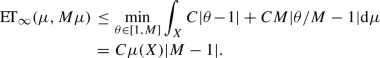  (46)

$\square$

The next Lemma shows the existence of the optimal couplings.

Lemma 6

Let be a regular Entropy-Transport distance induced by $(a,F,\ell )$. Let $(X_1,{\textsf {d} }_1,\mu _1)$ and $(X_2,{\textsf {d} }_2,\mu _2)$ be two metric measure spaces. Then:

• (i) here exist a measure $\varvec{\gamma }\in {\mathscr {M}}(X_1\times X_2)$ and a pseudo-metric coupling ${\hat{\textsf {d} }}$ between ${\textsf {d} }_1$ and ${\textsf {d} }_2$ such that

  

  (47)

• (ii) There exist a complete and separable metric space $({\tilde{X}},{\tilde{{\mathsf {d}}}})$ and isometric embeddings $\psi ^1:{\textsf {supp} }(\mu _1)\rightarrow {\tilde{X}}$, $\psi ^2:{\textsf {supp} }(\mu _2)\rightarrow {\tilde{X}}$ such that

  

  (48)

  where we have denoted by the Entropy-Transport distance computed in the space $({\tilde{X}},{\tilde{{\mathsf {d}}}})$.

Proof

• (i) $\mathbf {Step\, 1}$: tightness of the plans.

  By Proposition 2 there exist a sequence $\varvec{\gamma }_n\in {\mathscr {M}}(X_1\times X_2)$ and $\hat{{\mathsf {d}}}_n$ pseudo-metric couplings of ${\mathsf {d}}_1,{\mathsf {d}}_2$ such that

  

  (49)

  Since the entropy functionals with respect to the fixed measures $\mu _1$ and $\mu _2$ are bounded, we can apply Theorems 1 and Lemma 3 in order to obtain the existence of subsequences (from now on we will not relabel them) such that $(\gamma _n)_i$ converges weakly to some $\gamma ^i\in {\mathscr {M}}(X_i)$, $i=1,2$. Since $(\gamma _n)_i$ are marginals of the measure $\varvec{\gamma }_n$, the tightness of $(\gamma _n)_i$ implies the tightness of $\varvec{\gamma }_n$, so that the sequence $\varvec{\gamma }_n\in {\mathscr {M}}(X_1\times X_2)$ is converging to some $\varvec{\gamma }$. Moreover, by the continuity of the operator $\pi ^i_{\sharp }$ with respect to the weak topology, the marginals of $\varvec{\gamma }$ coincide with $\gamma ^i$, $i=1,2.$ We notice that if $\varvec{\gamma }$ is the null measure the proof is concluded by taking any pseudo-metric coupling $\hat{{\mathsf {d}}}$ between ${\mathsf {d}}_1$ and ${\mathsf {d}}_2$.

  $\mathbf {Step\, 2}$: pre-compactness of the pseudo-metric couplings.

  Regarding the sequence $\hat{{\mathsf {d}}}_n$, by the triangle inequality we have that

  $$\begin{aligned} |\hat{{\mathsf {d}}}_n(x_1,y_1)-\hat{{\mathsf {d}}}_n(x_2,y_2)|\le |{\mathsf {d}}_1(x_1,x_2)+{\mathsf {d}}_2(y_1,y_2)|. \end{aligned}$$

  In particular, $\hat{{\mathsf {d}}}_n$ is uniformly 1-Lipschitz with respect to the complete and separable metric ${\mathsf {d}}_1+{\mathsf {d}}_2$ on $X_1\times X_2$. We claim it is also uniformly bounded in a point. To see this, take $({\bar{x}},{\bar{y}})\in {\mathsf {supp}}(\varvec{\gamma })$: since $\varvec{\gamma }_n$ weakly converges to $\varvec{\gamma }$ for every $r,\epsilon >0$ and for all n sufficiently large we have

  $$\begin{aligned} \varvec{\gamma }_n\left( B_r({\bar{x}})\times B_r({\bar{y}})\right) \ge \varvec{\gamma }\left( B_r({\bar{x}})\times B_r({\bar{y}})\right) -\epsilon . \end{aligned}$$

  Fix $r>0$ and suppose by contradiction that there exists a subsequence (not relabeled) such that $2r\le \hat{{\mathsf {d}}}_n({\bar{x}},{\bar{y}})\rightarrow +\infty$. For $\epsilon =\epsilon (r)$ small enough, from (49), the fact that $({\bar{x}},{\bar{y}})\in {\mathsf {supp}}(\varvec{\gamma })$ and $\ell$ is increasing we infer the existence of some positive constants C, c such that for all n sufficiently large

  $$\begin{aligned}&C>\int _{X_1\times X_2}\ell \left( \hat{{\mathsf {d}}}_n(x,y)\right) {\mathrm d}\varvec{\gamma }_n(x,y)\\&\quad \ge \int _{B_r({\bar{x}})\times B_r({\bar{y}})}\ell \left( \hat{{\mathsf {d}}}_n({\bar{x}},{\bar{y}})-2r\right) {\mathrm d}\varvec{\gamma }_n(x,y)\\&\quad \ge \ell \left( \hat{{\mathsf {d}}}_n({\bar{x}},{\bar{y}})-2r\right) [\varvec{\gamma }(B_r({\bar{x}})\times B_r({\bar{y}}))-\epsilon ]\ge c\ell \left( \hat{{\mathsf {d}}}_n({\bar{x}},{\bar{y}})-2r\right) . \end{aligned}$$

  Since $\ell$ has bounded sublevels, this implies that there exists a constant K such that $\hat{{\mathsf {d}}}_n({\bar{x}},{\bar{y}})<K$ for every n that leads to a contradiction.

  We can thus apply Ascoli-Arzelà’s theorem to infer the existence of a limit function ${\mathsf {d}}:X_1\times X_2\rightarrow [0,\infty )$ such that ${\mathsf {d}}_n$ converges (up to subsequence) pointwise to ${\mathsf {d}}$ and the convergence is uniform on compact sets. We can extend ${\mathsf {d}}$ to $(X_1 \sqcup X_2)\times (X_1 \sqcup X_2)$ in order to get a limit pseudo-metric coupling, that we denote in the same way.

  $\mathbf {Step\, 3}$: passing to the limit.

  Next, we pass to the limit in the following expression

  $$\begin{aligned} \sum _{i=1}^2D_F((\gamma _n)_i||\mu _i)+\int _{X_1\times X_2}\ell \left( \hat{{\mathsf {d}}}_n(x,y)\right) {\mathrm d}\varvec{\gamma }_n. \end{aligned}$$

  By Lemma 2, the entropy is jointly lower semicontinuous and thus

  $$\begin{aligned} \liminf _n D_F((\gamma _n)_i||\mu _i)\ge D_F(\gamma _i||\mu _i). \end{aligned}$$

  So, it is sufficient to prove that

  $$\begin{aligned} \liminf _n \int _{X_1\times X_2}\ell \left( \hat{{\mathsf {d}}}_n(x,y)\right) {\mathrm d}\varvec{\gamma }_n \ge \int _{X_1\times X_2}\ell \left( \hat{{\mathsf {d}}}(x,y)\right) {\mathrm d}\varvec{\gamma }. \end{aligned}$$

  (50)

  Using the equi-tightness of $\{\varvec{\gamma }_k\}$ we can find a sequence of compact sets $K_{1,n}\subset X_1$ and $K_{2,n}\subset X_2$ such that

  $$\begin{aligned} \varvec{\gamma }_k\left( X_1\times X_2 {\setminus } (K_{1,n}\times K_{2,n})\right) \le \frac{1}{n} \end{aligned}$$

  for every k. We define $\ell _m(r):=\min (\ell (r),m),$ so that the sequence of functions $(x,y)\mapsto \ell _m({\mathsf {d}}_n(x,y))$ converges uniformly on compact subsets of $X_1\times X_2$, as $n\rightarrow \infty$. Possibly by taking a further subsequence via a diagonal argument, we can infer that $\Vert \ell _m({\mathsf {d}})-\ell _m({\mathsf {d}}_n)\Vert _{\infty ;n}\rightarrow 0$ when $n\rightarrow \infty$, where we denote by $\Vert \cdot \Vert _{\infty ;n}$ the supremum norm in the set $K_{1,n}\times K_{2,n}.$ Let M be a positive constant such that $\gamma _n(X_1\times X_2)\le M$ for every n. We can bound the integral on the left hand side of (50) in the following way:

  $$\begin{aligned}&\int _{X_1\times X_2} \ell (\hat{{\mathsf {d}}}_n) {\mathrm d}\varvec{\gamma }_n \ge \int _{X_1\times X_2} \ell _m(\hat{{\mathsf {d}}}_n) {\mathrm d}\varvec{\gamma }_n \ge \int _{K^1_n\times K^2_n} \ell _m(\hat{{\mathsf {d}}}_n) {\mathrm d}\varvec{\gamma }_n \\&\quad \ge \int _{K^1_n\times K^2_n} \ell _m(\hat{{\mathsf {d}}}) {\mathrm d}\varvec{\gamma }_n - M \Vert \ell _m(\hat{{\mathsf {d}}})-\ell _m(\hat{{\mathsf {d}}}_n)\Vert _{\infty ;n} \\&\quad \ge \int _{X_1\times X_2} \ell _m(\hat{{\mathsf {d}}}) {\mathrm d}\varvec{\gamma }_n - M \Vert \ell _m(\hat{{\mathsf {d}}})-\ell _m(\hat{{\mathsf {d}}}_n)\Vert _{\infty ;n} - m /n. \end{aligned}$$

  Now we can pass to the limit with respect to n using the weak convergence of $\{\varvec{\gamma }_n\}$, and we obtain

  $$\begin{aligned} \liminf _{n} \int _{X_1\times X_2} \ell (\hat{{\mathsf {d}}}_n) {\mathrm d}\varvec{\gamma }_n\ge \int _{X_1\times X_2} \ell _m(\hat{{\mathsf {d}}}) {\mathrm d}\varvec{\gamma } \end{aligned}$$

  and then we conclude using the Beppo Levi’s monotone convergence theorem with respect to m.

• (ii) Without loss of generality we assume ${\mathsf {supp}}(\mu _i)=X_i$. By the previous point we know the existence of an optimal measure $\varvec{\gamma }\in {\mathscr {M}}(X_1\times X_2)$ and an optimal pseudo-metric coupling $\hat{{\mathsf {d}}}$ between ${\mathsf {d}}_1$ and ${\mathsf {d}}_2$. We consider the complete and separable metric space $({\tilde{X}},{\tilde{{\mathsf {d}}}})$ constructed as in Lemma 1. Denoting by $p: X_1\sqcup X_2\rightarrow {\tilde{X}}$ the projection to the quotient and using the identification

  $$\begin{aligned} X_1\sqcup X_2=X_1\times \{0\}\cup X_2\times \{1\}, \end{aligned}$$

  we notice that $X_1\times X_2 \hookrightarrow {\tilde{X}} \times {\tilde{X}}$ via the injective Borel map

  $$\begin{aligned} \varvec{\psi }(x_1,x_2)=(\psi ^1(x_1),\psi ^2(x_2)):=(p(x_1,0),p(x_2,1)). \end{aligned}$$

  Moreover, we also have that $\psi ^i$ is an isometry of $(X_i,{\mathsf {d}}_i)$ onto its image in $({\tilde{X}},{\tilde{{\mathsf {d}}}})$, $i=1,2$. Thus, denoting by $\gamma _i$ the marginals of $\varvec{\gamma }$, we can consider the measures $\varvec{\psi }_{\sharp }\varvec{\gamma }$ whose projections are $(\psi ^1)_{\sharp }\gamma _1$ and $(\psi ^2)_{\sharp }\gamma _2$. Using Lemma 4 we know that

  $$\begin{aligned} D_F(\gamma _i||\mu _i)=D_F((\psi ^i)_{\sharp }\gamma _i\,||\,(\psi ^i)_{\sharp }\mu _i), \qquad i=1,2. \end{aligned}$$

  (51)

  By recalling the definition of ${\tilde{{\mathsf {d}}}}$, we also have

  $$\begin{aligned} \int _{X_1\times X_2}\ell \left( \hat{{\mathsf {d}}}(x,y)\right) {\mathrm d}\varvec{\gamma }=\int _{{\tilde{X}}\times {\tilde{X}}}\ell \left( {\tilde{{\mathsf {d}}}}(x,y)\right) {\mathrm d}(\varvec{\psi }_{\sharp }\varvec{\gamma }). \end{aligned}$$

  (52)

  Thus, as a consequence of (51), (52) and the optimality of $\varvec{\gamma }$ and ${\hat{{\mathsf {d}}}}$, the equality (48) holds on $({\tilde{X}},{\tilde{{\mathsf {d}}}})$ (with optimal measure $\varvec{\psi }_{\sharp }\varvec{\gamma }$).

$\square$

Remark 2

It is clear that the optimal coupling $\hat{{\mathsf {d}}}$ whose existence is proven in the previous Lemma is in general only a pseudo-metric and not a metric on $X_1\sqcup X_2$. To see this, it is sufficient to consider two isomorphic metric measure spaces $(X_1,{\mathsf {d}}_1,\mu _1)$, $(X_2,{\mathsf {d}}_2,\mu _2)$. If we denote by $\psi :X_1\rightarrow X_2$ the isometry between $(X_1,{\mathsf {d}}_1)$ and $(X_2,{\mathsf {d}}_2)$, the optimal coupling $\hat{{\mathsf {d}}}$ satisfies ${\hat{{\mathsf {d}}}}(x_1,\psi (x_1))=0$ for $\mu _1$-a.e $x_1$.

The next theorem is the main result of the paper.

Theorem 2

Let be a regular Entropy-Transport distance induced by $(a,F,\ell )$. Then is a complete and separable metric space. It is also a length (resp. geodesic) space if is a length (resp. geodesic) metric.

Proof

$\mathbf {Step\, 1}$: defines a metric.

It is clear that is symmetric, finite valued, nonnegative and

We claim that implies that the metric measure spaces $(X_1,{\mathsf {d}}_1,\mu _1)$ and $(X_2,{\mathsf {d}}_2,\mu _2)$ are isomorphic. By Lemma 6 there exist a measure $\varvec{\gamma }\in {\mathscr {M}}(X_1\times X_2)$ and a pseudo-metric coupling $\hat{{\mathsf {d}}}$ such that

$$\begin{aligned} 0=\sum _{i=1}^2D_F\left( \gamma _i||\mu _i\right) +\int _{X_1\times X_2}\ell \left( \hat{{\mathsf {d}}}(x,y)\right) {\mathrm d}\varvec{\gamma }. \end{aligned}$$

All the terms are nonnegative, so that $D_F\big (\gamma _i||\mu _i\big )=0$ and thus $\gamma _i=\mu _i$, $i=1,2$. Moreover, since $\ell (d)=0$ if and only if $d=0$, it follows that $\hat{{\mathsf {d}}}(x,y)=0$ for $\varvec{\gamma }$-a.e (x, y). We also have

$$\begin{aligned} \hat{{\mathsf {d}}}(x,y)=0 \quad \text {for all } (x,y)\in {\mathsf {supp}}(\varvec{\gamma }). \end{aligned}$$

(53)

To see this, let $({\bar{x}},{\bar{y}})\in {\mathsf {supp}}(\varvec{\gamma })$ so that for every $r>0$ we have $\varvec{\gamma }(B_r({\bar{x}},{\bar{y}}))>0$ where

$$\begin{aligned} B_r(({\bar{x}},{\bar{y}}))=\{(x,y)\in X_1\times X_2\,|\, {\mathsf {d}}_1({\bar{x}},x)+{\mathsf {d}}_2({\bar{y}},y)<r\}. \end{aligned}$$

We consider a sequence of balls of radius $r_n:=1/n, n\in {\mathbb {N}},$ and use the fact that $\hat{{\mathsf {d}}}(x,y)=0$ for $\varvec{\gamma }$-a.e (x, y) to infer the existence of a sequence of points $(x_n, y_n)\in B_{r_n}(({\bar{x}},{\bar{y}}))$ such that $\hat{{\mathsf {d}}}(x_n,y_n)=0$. Thus

$$\begin{aligned} \hat{{\mathsf {d}}}({\bar{x}},{\bar{y}})\le {\mathsf {d}}_1({\bar{x}},x_n)+\hat{{\mathsf {d}}}(x_n,y_n)+{\mathsf {d}}_2({\bar{y}},y_n)<1/n. \end{aligned}$$

Sending $n\rightarrow +\infty$ and using the arbitrariness of $({\bar{x}},{\bar{y}})$, the claim (53) follows.

Since ${\mathsf {d}}_1$ and ${\mathsf {d}}_2$ are metrics, we infer that for every $x_{1}\in {\mathsf {supp}}(\mu _{1})$ there exists a unique $x_{2}\in {\mathsf {supp}}(\mu _{2})$ such that $(x_{1},x_{2})\in {\mathsf {supp}}(\varvec{\gamma })$. Indeed, for any $x_2,{\tilde{x}}_{2}\in {\mathsf {supp}}(\mu _{2})$ such that $(x_{1},x_{2}), (x_{1},{\tilde{x}}_{2})\in {\mathsf {supp}}(\varvec{\gamma })$ we have

$$\begin{aligned} {\mathsf {d}}_2(x_2,{\tilde{x}}_{2})=\hat{{\mathsf {d}}}(x_2,{\tilde{x}}_{2})\le \hat{{\mathsf {d}}}(x_{2},x_1)+\hat{{\mathsf {d}}}({\tilde{x}}_{2}, x_1)=0 \end{aligned}$$

and thus $x_2={\tilde{x}}_2$. Switching the role of $X_{1}$ and $X_{2}$ in the argument above, we obtain the existence of a bijection $\psi : {\mathsf {supp}}(\mu _{1}) \rightarrow {\mathsf {supp}}(\mu _{2})$ such that $\varvec{\gamma }=(\mathrm {Id},\psi )_{\sharp }\mu _1$ and (in virtue of (53))

$$\begin{aligned} \hat{{\mathsf {d}}}(x,\psi (x))=0 \quad \text {for all } x\in {\mathsf {supp}}(\mu _{1}). \end{aligned}$$

(54)

Let $x,y\in {\mathsf {supp}}(\mu _{1})$, from (54) and the triangle inequality it follows

$$\begin{aligned} \begin{aligned} {\mathsf {d}}_1(x,y)&=\hat{{\mathsf {d}}}(x,y)\le \hat{{\mathsf {d}}}(x,\psi (x))+\hat{{\mathsf {d}}}(\psi (x),\psi (y))+\hat{{\mathsf {d}}}(y,\psi (y))\\&={\mathsf {d}}_{2}(\psi (x),\psi (y)),\\ {\mathsf {d}}_{2}(\psi (x),\psi (y))&=\hat{{\mathsf {d}}}(\psi (x),\psi (y))\le \hat{{\mathsf {d}}}(x,\psi (x))+\hat{{\mathsf {d}}}(x,y)+\hat{{\mathsf {d}}}(y,\psi (y))\\&={\mathsf {d}}_1(x,y), \end{aligned} \end{aligned}$$

which implies that $\psi : {\mathsf {supp}}(\mu _{1}) \rightarrow {\mathsf {supp}}(\mu _{2})$ is an isometry.

Hence $(X_1,{\mathsf {d}}_1,\mu _1)$ and $(X_2,{\mathsf {d}}_2,\mu _2)$ are isomorphic, as claimed.

Regarding the triangle inequality, let $(X_i,{\mathsf {d}}_i,\mu _i)$, $i=1,2,3$, be three metric measure spaces. From the definition of and Proposition 2, for every $\epsilon >0$ we find a pseudo-metric coupling ${\mathsf {d}}_{12}$ between ${\mathsf {d}}_{1}$ and ${\mathsf {d}}_{2}$, and a pseudo-metric coupling ${\mathsf {d}}_{23}$ between ${\mathsf {d}}_{2}$ and ${\mathsf {d}}_{3}$ such that

where we have denoted by the Entropy-Transport distance induced by the pseudo-metric ${\mathsf {d}}$. Set $X:=X_1\sqcup X_2\sqcup X_3$ and define a pseudo-metric ${\mathsf {d}}$ on X in the following way

$$\begin{aligned} {\mathsf {d}}(x,y):={\left\{ \begin{array}{ll} {\mathsf {d}}_{12}(x,y) \ \ \ \ \ &{}\text {if} \ x,y\in X_1\sqcup X_2 \\ {\mathsf {d}}_{23}(x,y) \ \ \ \ \ &{}\text {if} \ x,y\in X_2\sqcup X_3 \\ \inf _{z\in X_2}[{\mathsf {d}}_{12}(x,z)+{\mathsf {d}}_{23}(z,y)] \ \ &{}\text {if} \ x\in X_1 \ \text {and} \ y\in X_3\\ \inf _{z\in X_2}[{\mathsf {d}}_{23}(x,z)+{\mathsf {d}}_{12}(z,y)] \ \ &{}\text {if}\ x\in X_3 \ \text {and} \ y\in X_1. \end{array}\right. } \end{aligned}$$

We notice that ${\mathsf {d}}$ coincides with ${\mathsf {d}}_i$ when restricted to $X_i$. By applying Proposition 2, the point (ii) of Lemma 5 and the triangle inequality of we obtain

The conclusion follows since $\epsilon >0$ is arbitrary.

$\mathbf {Step\, 2}$: Completeness of .

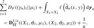
In order to prove completeness, let $\{(X_n,{\mathsf {d}}_n,\mu _n)\}_{n\in {\mathbb {N}}}$ be a Cauchy sequence in the space . In order to have convergence of the full sequence, it is enough to prove that there exists a converging subsequence. Let us consider a subsequence such that

By definition of and Proposition 2, we can find a measure $\varvec{\gamma }_{k+1}\in {\mathscr {M}}(X_{n_k}\times X_{n_{k+1}})$ and a complete and separable metric coupling $\hat{{\mathsf {d}}}_{k+1}$ between ${\mathsf {d}}_{X_{n_k}}$ and ${\mathsf {d}}_{X_{n_{k+1}}}$ such that

$$\begin{aligned}&\int _{X_{n_k}} F(\sigma _{n_k}){\mathrm d}\mu _{n_k}+\int _{X_{n_{k+1}}} F(\sigma _{n_{k+1}}){\mathrm d}\mu _{n_{k+1}}\nonumber \\&\quad +\int _{X_{n_k}\times X_{n_{k+1}}}\ell \left( \hat{{\mathsf {d}}}_{k+1}\right) {\mathrm d}\varvec{\gamma }_{k+1}<2^{-k}, \end{aligned}$$

(55)

where $\sigma _{n_k}$ (resp. $\sigma _{n_{k+1}}$) is the Radon-Nykodim derivative of the first (resp. second) marginal of $\gamma _{k+1}$ with respect to $\mu _{n_k}$ (resp. $\mu _{n_{k+1}}$).

Now we want to define a sequence $\big \{(X'_k,{\mathsf {d}}'_k)\big \}_{k=1}^{\infty }$ of metric spaces such that $X_{n_k}\subset X'_k$ and $X'_k\subset X'_{k+1}$. We proceed in the following way: we set

$$\begin{aligned} \left( X'_1,{\mathsf {d}}'_1\right)&:=\left( X_{n_1},{\mathsf {d}}_{X_{n_1}}\right) , \\ X'_{k+1}&:=X'_k\sqcup X_{n_{k+1}} \big / \sim , \end{aligned}$$

where $x\sim y$ if ${\mathsf {d}}'_{k+1}(x,y)=0$ and the latter is defined as

$$\begin{aligned} {\mathsf {d}}'_{k+1}(x,y):= {\left\{ \begin{array}{ll} {\mathsf {d}}'_{k}(x,y) \ \ &{}\text {if} \ \ x,y\in X'_k\\ \hat{{\mathsf {d}}}_{k+1}(x,y) \ \ &{}\text {if} \ \ x,y\in X_{n_k}\sqcup X_{n_{k+1}} \\ \inf _{z\in X_{n_k}}{\mathsf {d}}'_{k}(x,z)+\hat{{\mathsf {d}}}_{k+1}(z,y) \ \ &{}\text {if} \ \ x\in X'_k,\, y\in X_{n_{k+1}}\\ \inf _{z\in X_{n_k}}{\mathsf {d}}'_{k}(y,z)+\hat{{\mathsf {d}}}_{k+1}(z,x) \ \ &{}\text {if} \ \ y\in X'_k,\, x\in X_{n_{k+1}}. \end{array}\right. } \end{aligned}$$

From the definition of ${\mathsf {d}}'_k$, it is clear that we can endow the space $X':=\bigcup _{k=1}^{\infty } X'_k$ with a limit metric ${\mathsf {d}}'$. Now we consider the completion $(X,{\mathsf {d}})$ of $(X',{\mathsf {d}}')$ and we notice that $(X_{n_k},{\mathsf {d}}_{X_{n_k}})$ is isometrically embedded in this space for every k. Using the embedding, we can also define a measure ${\bar{\mu }}_{n_k}$ as the push-forward of the measure $\mu _{n_k}.$ Combining the construction above with (55) gives

(56)

where is the regular Entropy-Transport distance computed in the space $(X,{\mathsf {d}}).$ In particular, (56) implies that $({\bar{\mu }}_{n_{k}})_{k\in {\mathbb {N}}}$ is a Cauchy sequence in . Since is complete, there exists $\mu \in {\mathscr {M}}(X)$ such that .

Using again that $(X_{n_k},{\mathsf {d}}_{X_{n_k}})$ is isometrically embedded in $(X,{\mathsf {d}})$ and the point (ii) of Lemma 5, we can conlude that

(57)

$\mathbf {Step\, 3}$: Separability of .

Thanks to (iii) of Lemma 5 it is enough to show that the set $\varvec{\mathrm {X}}_*$, defined in (41), is separable. To this aim, we notice that $\varvec{\mathrm {X}}_*$ can be written as $\bigsqcup _{n\in {\mathbb {N}}} \tilde{{\mathcal {K}}}_n$ where

$$\begin{aligned} \tilde{{\mathcal {K}}}_n:=\{(X,{\mathsf {d}},\mu )\in \varvec{\mathrm {X}}_*: {\mathsf {supp}}(\mu ) \ \text {has} \ n \ \text {points}\}. \end{aligned}$$

Since the set of all $(D,M)=(D_{ij},M)\in {\mathbb {R}}_+^{n\times n}\times {\mathbb {R}}_{+}$ such that

$$\begin{aligned} D_{ij}=D_{ji} \, , \ \ D_{ij}=0 \iff i=j\, , \ \ D_{ij}\le D_{ik}+D_{kj}\, \end{aligned}$$

(58)

is separable (as a subset of the Euclidean space), using (iv) of Lemma 5 we get that

$$\begin{aligned} \tilde{{\mathcal {K}}}_{n,M}:=\{(X,{\mathsf {d}},\mu )\in \varvec{\mathrm {X}}_*: {\mathsf {supp}}(\mu ) \ \text {has} \ n \ \text {points and } \mu (X)=nM\} \end{aligned}$$

is separable for every fixed $n\in {{\mathbb {N}}}, M>0$. The separability of $\tilde{{\mathcal {K}}}_n$ follows by the separability of $\tilde{{\mathcal {K}}}_{n,M}$ combined with (v) of Lemma 5.

$\mathbf {Step\, 4}$: Length/geodesic property of .

Let us start by proving the length property. Let $(X_1,{\mathsf {d}}_1,\mu _1),\, (X_2,{\mathsf {d}}_2,\mu _2) \in \varvec{\mathrm {X}}$. By definition of , for every $\varepsilon >0$ we can find a complete and separable metric space $(X, {\mathsf {d}})$ and isometric embeddings $\psi ^i: {\mathsf {supp}}(\mu _i) \rightarrow X$, $i=1,2$, such that

(59)

where, as before, we identify ${\mathsf {supp}}(\mu _i)$ with its isometric image $\psi ^i({\mathsf {supp}} (\mu _i))$, and correspondingly $\mu _i$ with $\psi ^i_\sharp \mu _{i}$, $i=1,2$, in order to keep notation short.

Recall that, by slightly modifying the classical Kuratowski embedding, one can show that every complete and separable metric space can be isometrically embedded in a complete, separable and geodesic metric space (see for instance [23,  Exercise 1c. Ch. 3$\frac{1}{2}.1$] or [22,  Proposition 1.2.12]). Thus, recalling also Lemma 4, without loss of generality we can assume that the complete and separable metric space $(X,{\mathsf {d}})$ above is also geodesic.

By assumption is a length distance on ${\mathscr {M}}(X)$ since $(X,{\mathsf {d}})$ is a length space, so that we can find a curve from $\mu _1$ to $\mu _2$ satisfying

(60)

Now, it is easy to check that the -length of the curve of m.m.s. $((X, {\mathsf {d}}, \mu _{t}))_{t\in [1,2]}\subset \varvec{\mathrm {X}}$ satisfies

(61)

Indeed the length of a curve is by definition the supremum of the sums of mutual distances over finite partitions (13), and for every partition $(t_{i})$ of [1, 2] it holds

The combination of (59), (60) and (61) gives

as desired.

To prove the geodesic property in the case is a geodesic distance, we notice that we can follow verbatim the argument given above with $\varepsilon =0$. Here one has to notice that the existence of an optimal complete and separable metric space on which (59) holds with $\varepsilon =0$ follows from (ii) of Lemma 6. $\square$

Remark 3

It is proved in [29,  Proposition 8.3] that is a geodesic space when the underlying space $(X,{\mathsf {d}})$ is geodesic. In particular, the last claim of Theorem 2 can be applied to the Hellinger-Kantorovich distance.

To the best of our knowledge, up to now this is the only known example of regular Entropy-Transport geodesic distance (with the trivial exception of weighted variants of [28]).

4.1 Topology

Let us introduce a notion of convergence for sequences of (equivalence classes of) metric measure spaces (see [21,  Definition 3.9] for the corresponding notion in the context of pointed metric measure spaces).

Definition 5

We say that a sequence $(X_n,{\mathsf {d}}_n,\mu _n)_{n\in {\mathbb {N}}}$ weakly measured-Gromov converges to $(X_{\infty },{\mathsf {d}}_{\infty },\mu _{\infty })$ if there exist a complete and separable metric space $(X,{\mathsf {d}})$ and isometric embeddings $\iota _n:X_n\rightarrow X$, $n\in \bar{{\mathbb {N}}}$, such that $(\iota _n)_{\sharp }\mu _n \rightarrow (\iota _{\infty })_{\sharp }\mu _{\infty }$ weakly in ${\mathscr {M}}(X)$.

In the next Theorem we see that this notion of convergence actually coincides with the convergence induced by any Sturm-Entropy-Transport distance.

Theorem 3

Let be a regular Entropy-Transport distance induced by $(a,F,\ell )$. A sequence $(X_n,{\textsf {d} }_n,\mu _n)_{n\in {\mathbb {N}}}$ weakly measured Gromov converges to $(X_{\infty },{\textsf {d} }_{\infty },\mu _{\infty })$ if and only if

(62)

Proof

Let us suppose the validity of (62). By definition of we know that there exist a complete and separable metric space $(Y_n,{\mathsf {d}}_{Y_n})$ and isometric embeddings $\psi _n,\psi _n^{\infty }$ of $(X_n,{\mathsf {d}}_n)$, $(X_{\infty },{\mathsf {d}}_{\infty })$ respectively, in $Y_n$ such that

(63)

where is computed in the space $Y_n$. We now define $Y:=\sqcup _n X_n$, $n\in \bar{{\mathbb {N}}}$ endowed with the pseudo-metric ${\mathsf {d}}_Y$

$$\begin{aligned} {\mathsf {d}}_Y(y,y'):= {\left\{ \begin{array}{ll} {\mathsf {d}}_{n}(y,y') \ \ &{}\text {if} \ \ y,y'\in X_n, n\in \bar{{\mathbb {N}}}\\ {\mathsf {d}}_{Y_n}(\psi _n(y),\psi _n^{\infty }(y')) \ \ &{}\text {if} \ \ y\in X_{n}, \, y' \in X_{\infty } \\ {\mathsf {d}}_{Y_n}(\psi _n^{\infty }(y), \psi _n(y')) \ \ &{}\text {if} \ y \in X_{\infty }, \, y'\in X_{n} \\ \inf _{x\in X_{\infty }}{\mathsf {d}}_{Y_n}(\psi _n(y), \psi _n^{\infty }(x))+{\mathsf {d}}_{Y_m}(\psi _m(y'), \psi _m^{\infty }(x)) \ \ &{}\text {if} \ \ y\in X_n,\, y'\in X_{m}. \end{array}\right. } \end{aligned}$$

We now consider the space $Y/\sim$ defined as the quotient of Y with respect to the equivalence relation

$$\begin{aligned} y\sim y' \Leftrightarrow {\mathsf {d}}_Y(y,y')=0 \, , \end{aligned}$$

(64)

and we then define the completion of this space, that we still denote by $(Y,{\mathsf {d}}_Y)$. It is easy to see that Y is separable. By construction we notice that the set

$$\begin{aligned} \psi _n(X_n)\cup \psi _n^{\infty }(X_{\infty })\subset Y_n \end{aligned}$$

endowed with the distance ${\mathsf {d}}_{Y_n}$ is canonically isometrically embedded in $(Y,{\mathsf {d}}_Y)$, so that every space $X_n$, $n\in \bar{{\mathbb {N}}}$, is canonically isometrically embedded into Y by a map $\psi _n'$. We claim now that Y and $\psi _n'$ provide a realization of the weakly measured Gromov convergence. To see this, it is enough to notice that $(\psi _n')_{\sharp }\mu _n\rightarrow (\psi _{\infty }')_{\sharp }\mu _{\infty }$ weakly in ${\mathscr {M}}(Y)$ which is a consequence of the construction of $\psi _n'$, (63) and the fact that induces the weak topology.

For the converse, let us suppose that $(X_n,{\mathsf {d}}_n,\mu _n)_{n\in {\mathbb {N}}}$ weakly measured Gromov converges to $(X_{\infty },{\mathsf {d}}_{\infty },\mu _{\infty })$. By definition we know that there exist a complete and separable metric space $(X,{\mathsf {d}})$ and isometric embeddings $\iota _n:X_n\rightarrow X$, $n\in \bar{{\mathbb {N}}}$, such that $(\iota _n)_{\sharp }\mu _n \rightarrow (\iota _{\infty })_{\sharp }\mu _{\infty }$ weakly in ${\mathscr {M}}(X)$. Since metrizes the weak convergence on ${\mathscr {M}}(X)$ we know that

and the result follows by the very definition of , noticing that $(X,{\mathsf {d}})$ is a possible competitor. $\square$

Let us denote by $\varvec{\mathrm {X}}(K,N,L,v,V)$ the family of isomorphism classes of metric measure spaces $(X,{\mathsf {d}},\mu ) \in {\mathsf {CD}}(K,N)$ such that

$$\begin{aligned} \mathsf {diam}(X)\le L \quad \text {and} \quad 0<v\le \mu (X)\le V. \end{aligned}$$

Let $\varvec{\tilde{\mathrm {X}}}(K,N,L,v,V)$ be the family of isomorphism classes of spaces

$$\begin{aligned} (X,{\mathsf {d}},\mu )\in \varvec{\mathrm {X}}(K,N,L,v,V) \end{aligned}$$

such that $\mu$ has full support.

Theorem 4

Fix $K\in {\mathbb {R}}$, $N\in (1,\infty )$, $L\in (0,\infty )$ and $0<v\le V<\infty$. Let be a regular Entropy-Transport distance. Then

• $\varvec{\mathrm {X}}(K,N,L,v,V)$ is compact with respect to .

• $\varvec{\tilde{\mathrm {X}}}(K,N,L,v,V)$ is compact with respect to mGH. Moreover on such family the -topology and the mGH-topology coincide.

Proof

By [21,  Corollary 3.22] we have precompactness of $\varvec{\mathrm {X}}(K,N,L,v,V)$ with respect to the weakly measured Gromov convergence and thus precompactness with respect also to the -convergence by Theorem 3. From [44,  Theorem 3.1] (see also [21,  Theorem 4.9]) we know that the condition ${\mathsf {CD}}(K,N)$ is stable with respect to the weakly measured Gromov convergence and thus the first statement follows. For the second statement we observe that the spaces in $\varvec{\tilde{\mathrm {X}}}(K,N,L,v,V)$ are uniformly doubling and thus the weakly measured Gromov convergence is equivalent to the mGH-convergence (see [21,  Theorem 3.30 and 3.33]). $\square$

Corollary 1

It follows:

• (i) The stability of ${\textsf {CD} }(K,N)$ with $N\in (1,\infty ]$ under -convergence.

• (ii) The convergence of heat flows under -convergence of ${\textsf {CD} }(K,\infty )$ spaces.

• (iii) The stability of ${\textsf {RCD} }(K,N)$ with $N\in (1,\infty ]$ under -convergence.

• (iv) The stability of the spectrum of the Laplacian under -convergence of ${\textsf {CD} }(K,\infty )$ spaces.

Proof

The proof is a direct consequence of Theorem 3 and the results contained in [21], to which we refer for the precise statements. In particular, for (i) we use [21,  Theorem I and pp. 29-30], (ii) follows from [21,  Theorem 5.7], for (iii) we take advantage of [21,  Theorem IV], and (iv) is a consequence of [21,  Theorem V]. $\square$

5 Limiting cases

5.1 Pure entropy distances

In the setting of Entropy-Transport problems, we call pure entropy problems the ones induced by the choices

$$\begin{aligned} F\in \Gamma _0({\mathbb {R}}_+), \qquad \varvec{\mathrm c}(x_1,x_2)={\left\{ \begin{array}{ll}0 \ &{}\text {if} \ x_1=x_2, \\ +\infty &{}\text {otherwise.} \end{array}\right. } \end{aligned}$$

In this situation one can prove (see [29,  Example E.5]) that for any $\mu _1,\mu _2\in {\mathscr {M}}(X)$ we have

(65)

where $\lambda \in {\mathscr {M}}(X)$ is any dominating measure of $\mu _1$ and $\mu _2$ and $H_0$ is defined as the lower semicontinuous envelope of the function

$$\begin{aligned} {\tilde{H}}_0(r,t):=\inf _{\theta >0} {\hat{F}}(\theta ,r)+{\hat{F}}(\theta ,t). \end{aligned}$$

(66)

In particular, the functional corresponds in this situation to the Csiszár’s divergence induced by the function $s\mapsto H_0(1,s)\in \Gamma _0({\mathbb {R}}_+)$ (see [14,  Lemma 3]), justifying the name of pure entropy problem.

For some entropy functions F one can prove that a power a of the induced pure entropy cost is a distance. For instance, when $a=1$ and $F(s)=|s-1|$ we obtain the celebrated total variation (denoted by $\mathsf {TV}$ in the sequel), a distance in the space of measures inducing a strong topology. Actually, thanks to the result proved in [14,  Lemma 8] and the explicit bounds contained in [31,  Theorem 2.5], we know that every pure entropy distance induces the same topology of the total variation.

As shown in [14,  Propositions 2, 3], we obtain another class of pure entropy distances by choosing $a=1/2$ and the power-like entropy $F=U_p$, $p\ge 1$, defined in example 3. In this situation we have

$$\begin{aligned} H_0(r,t)&=\frac{1}{p}\left[ r+t-2^{\frac{p}{p-1}}(r^{1-p}+t^{1-p})^{\frac{1}{1-p}}\right] \qquad \text {if} \ p>1, \end{aligned}$$

(67)

$$\begin{aligned} H_0(r,t)&=(\sqrt{r}-\sqrt{t})^2, \qquad p=1, \end{aligned}$$

(68)

and we recognize some well-known functionals like the 2-Hellinger distance (case $p=1$) and the triangular discrimination (case $p=2$). We will denote these distances by $\mathsf {PL}_{p}$.

We start with a useful lemma, valid for any pure entropy problem.

Lemma 7

Fix $a\in (0,1]$ and let us consider the functions

$$\begin{aligned} F\in \Gamma _0({\mathbb {R}}_+) \ \text {such that} \ F^{\prime }_{\infty }=+\infty , \qquad \varvec{\mathrm c}(x_1,x_2)={\left\{ \begin{array}{ll}0 \ &{}\text {if} \ x_1=x_2, \\ +\infty &{}\text {otherwise}. \end{array}\right. } \end{aligned}$$

Let us denote by ${\textsf {PE} }$ the power a of the Entropy-Transport cost induced by F and $\varvec{\mathrm c}$.

For any $(X_1,{\textsf {d} }_1,\mu _1),(X_2,{\textsf {d} }_2,\mu _2)\in \varvec{\mathrm {X}}$ let us define

$$\begin{aligned} {\mathbf {PE}}\left( (X_1,{\textsf {d} }_1,\mu _1),(X_2,{\textsf {d} }_2,\mu _2)\right) :=\inf {\textsf {PE} }(\psi ^1_{\sharp }\mu _1,\psi ^2_{\sharp }\mu _2), \end{aligned}$$

(69)

where the infimum in the right hand side is taken over all complete and separable metric spaces $({\hat{X}},{\hat{\textsf {d} }})$ with isometric embeddings $\psi ^1:{\textsf {supp} }(\mu _1)\rightarrow {\hat{X}}$ and $\psi ^2:{\textsf {supp} }(\mu _2)\rightarrow {\hat{X}}$.

Then

$$\begin{aligned} {\mathbf {PE}}^{1/a}\left( (X_1,{\textsf {d} }_1,\mu _1),(X_2,{\textsf {d} }_2,\mu _2)\right) = \inf _C\left\{ D_F(\gamma _1||\mu _1)+D_F(\gamma _2||\mu _2)\right\} , \end{aligned}$$

(70)

where

$$\begin{aligned} C:=\left\{ (\varvec{\gamma },{\hat{{\mathsf {d}}}}): \varvec{\gamma }\in {\mathscr {M}}(X_1\times X_2),\, {\hat{{\mathsf {d}}}} \ \text {pseudo-metric coupling for} \ {\mathsf {d}}_1,{\mathsf {d}}_2, \ {\textsf {supp} }(\varvec{\gamma })\subset \{{\hat{{\mathsf {d}}}}=0\} \right\} . \end{aligned}$$

Proof

Setting

$$\begin{aligned} \ell (d):={\left\{ \begin{array}{ll} 0 &{}\text {if} \ d=0\\ +\infty &{}\text {otherwise}, \end{array}\right. } \end{aligned}$$

we can prove that the infimum of

$$\begin{aligned} \left\{ D_F(\gamma _1||\mu _1)+D_F(\gamma _2||\mu _2)+\int _{X_1\times X_2}\ell \left( \hat{{\mathsf {d}}}(x,y)\right) {\mathrm d}\varvec{\gamma }\right\} ^a \end{aligned}$$

over the set

$$\begin{aligned} {\tilde{C}}:=\{(\varvec{\gamma },{\hat{{\mathsf {d}}}}): \varvec{\gamma }\in {\mathscr {M}}(X_1\times X_2),\, {\hat{{\mathsf {d}}}} \ \text {pseudo-metric coupling for} \ {\mathsf {d}}_1,{\mathsf {d}}_2\} \end{aligned}$$

is less or equal to the infimum in the right hand side of (69) by reasoning as in the first part of the Proof of Proposition 2. The fact that the power a of the right hand side of (70) is less or equal to the infimum as in (69) follows by noticing that

$$\begin{aligned} \int _{X_1\times X_2}\ell \left( \hat{{\mathsf {d}}}(x,y)\right) {\mathrm d}\varvec{\gamma }= {\left\{ \begin{array}{ll} +\infty \qquad &{}\text {if} \ {\mathsf {supp}}(\varvec{\gamma })\not \subset \{{\hat{{\mathsf {d}}}}=0\}\\ 0 &{}\text {otherwise}. \end{array}\right. } \end{aligned}$$

(71)

For the converse inequality, we reason in a similar way as in the proof of the point (ii) of Lemma 6. For any pseudo-metric coupling ${\hat{{\mathsf {d}}}}$ of ${\mathsf {d}}_1$ and ${\mathsf {d}}_2$ let us consider the space $((X_1\sqcup X_2)/\sim ,{\hat{{\mathsf {d}}}})$, where $x_1\sim x_2 \Longleftrightarrow {\hat{{\mathsf {d}}}}(x_1,x_2)=0.$ It is a complete and separable metric space as proved in Lemma 1. Denoting by $q: X_1\sqcup X_2\rightarrow (X_1\sqcup X_2)/\sim$ the projection to the quotient and using the identification

$$\begin{aligned} X_1\sqcup X_2=X_1\times \{0\}\cup X_2\times \{1\}, \end{aligned}$$

we notice that

$$\begin{aligned} X_1\times X_2 \hookrightarrow \left( (X_1\sqcup X_2)/\sim \right) \times \left( (X_1\sqcup X_2)/\sim \right) \end{aligned}$$

via the injective map

$$\begin{aligned} \varvec{\psi }(x_1,x_2)=(\psi ^1(x_1),\psi ^2(x_2)):=(q(x_1,0),q(x_2,1)). \end{aligned}$$

Moreover, we also have that $\psi ^i$ is an isomorphism of $(X_i,{\mathsf {d}}_i)$ into its image in $((X_1\sqcup X_2)/\sim ,{\hat{{\mathsf {d}}}})$, $i=1,2$. Thus, for any measure $\varvec{\gamma }\in {\mathscr {M}}(X_1\times X_2)$ such that ${\mathsf {supp}}(\varvec{\gamma })\subset \{{\hat{{\mathsf {d}}}}=0\}$, denoting by $\gamma _i$ the marginals of $\varvec{\gamma }$, we can consider the measures $\varvec{\psi }_{\sharp }\varvec{\gamma }$ whose projections are $(\psi ^1)_{\sharp }\gamma _1$ and $(\psi ^2)_{\sharp }\gamma _2$. Using Lemma 4 we know that

$$\begin{aligned} D_F(\gamma _i||\mu _i)=D_F((\psi ^i)_{\sharp }\gamma _i||(\psi ^i)_{\sharp }\mu _i), \qquad i=1,2 \end{aligned}$$

and the proof is completed by noticing that ${\mathsf {supp}}(\varvec{\psi }_{\sharp }\varvec{\gamma })$ is contained in the diagonal of the metric space $((X_1\sqcup X_2)/\sim ,{\hat{{\mathsf {d}}}})$. $\square$

In the next theorem we prove that some pure entropy problems, specifically the ones generated by power-like entropies $U_p$, $p\ge 1$, can be recovered as a limiting case of regular Entropy-Transport problems.

Theorem 5

Fix $p\ge 1$ and let us consider the sequence of cost functions $\varvec{\mathrm c}_n=n{\mathsf {d}}$ and the entropy function $F:=U_p$. Let us denote by ${\textsf {D} }_{p,n}$ the Entropy-Transport distance induced by $a=1/2$, $\varvec{\mathrm {c}}_n=n{\textsf {d} }$ and $F:=U_p$.

Then, for every metric measure spaces $(X_1,{\textsf {d} }_1,\mu _1)$, $(X_2,{\textsf {d} }_2,\mu _2)\in \varvec{\mathrm {X}}$ the limit

$$\begin{aligned} {\mathbf {PL}}_p\left( (X_1,{\textsf {d} }_1,\mu _1),(X_2,{\textsf {d} }_2,\mu _2)\right) :=\lim _{n \rightarrow \infty }{\mathbf {D}}_{p,n}\left( (X_1,{\textsf {d} }_1,\mu _1),(X_2,{\textsf {d} }_2,\mu _2)\right) \quad \text {is well defined},\nonumber \\ \end{aligned}$$

(72)

where ${\mathbf {D}}_{p,n}$ denotes the function defined as in Definition 4 upon replacing by ${\textsf {D} }_{p,n}$.

Moreover, ${\textsf {D} }_{p,n}$ is a regular Entropy-Transport distance and ${\mathbf {PL}}_p$ defines a metric on $\varvec{\mathrm {X}}$ such that

$$\begin{aligned} {\mathbf {PL}}_p\left( (X_1,{\textsf {d} }_1,\mu _1),(X_2,{\textsf {d} }_2,\mu _2)\right) =\inf {\textsf {PL} }_{p}(\psi ^1_{\sharp }\mu _1,\psi ^2_{\sharp }\mu _2), \end{aligned}$$

(73)

where the infimum in the right hand side is taken over all complete and separable metric spaces $({\hat{X}},{\hat{\textsf {d} }})$ with isometric embeddings $\psi ^1:{\textsf {supp} }(\mu _1)\rightarrow {\hat{X}}$ and $\psi ^2:{\textsf {supp} }(\mu _2)\rightarrow {\hat{X}}$.

Proof

The first assertion follows by noticing that for any metric ${\mathsf {d}}$ we have

$$\begin{aligned} n{\mathsf {d}}(x_1,x_2)\uparrow \varvec{\mathrm c}(x_1,x_2)={\left\{ \begin{array}{ll}0 \ &{}\text {if} \ x_1=x_2 \\ +\infty &{}\text {otherwise} \end{array}\right. } \qquad \text {as} \ n \rightarrow \infty \ \text {for every} \ x_1,x_2\in X.\nonumber \\\ \end{aligned}$$

(74)

The fact that ${\mathsf {D}}_{p,n}$ is a regular Entropy-Transport distance is a consequence of [14,  Theorem 6], noticing the obvious fact that $n{\mathsf {d}}$ is a complete and separable metric for any fixed n.

In particular, since for every fixed n we know that ${\mathbf {D}}_{p,n}$ is a metric on $\varvec{\mathrm {X}}$ by Theorem 2, we have that ${\mathbf {PL}}_p$ is nonnegative, symmetric, it satisfies the triangle inequality and

$$\begin{aligned} {\mathbf {PL}}_p\left( (X_1,{\mathsf {d}}_1,\mu _1),(X_2,{\mathsf {d}}_2,\mu _2)\right) =0 \quad \text {if} \quad (X_1,{\mathsf {d}}_1,\mu _1)=(X_2,{\mathsf {d}}_2,\mu _2). \end{aligned}$$

We claim that

$$\begin{aligned} {\mathbf {PL}}_p\left( (X_1,{\mathsf {d}}_1,\mu _1),(X_2,{\mathsf {d}}_2,\mu _2)\right) =0 \end{aligned}$$

only if $(X_1,{\mathsf {d}}_1,\mu _1)=(X_2,{\mathsf {d}}_2,\mu _2)$ (as equivalence classes). Indeed, since ${\mathbf {D}}_{p,n}$ is nonnegative and nondecreasing, the fact that

$$\begin{aligned} \lim _{n\rightarrow \infty }{\mathbf {D}}_{p,n}\left( (X_1,{\mathsf {d}}_1,\mu _1),(X_2,{\mathsf {d}}_2,\mu _2)\right) =0 \end{aligned}$$

implies

$$\begin{aligned} {\mathbf {D}}_{p,n}\left( (X_1,{\mathsf {d}}_1,\mu _1),(X_2,{\mathsf {d}}_2,\mu _2)\right) =0 \qquad \text {for every} \ n, \end{aligned}$$

and the result follows because ${\mathbf {D}}_{p,n}$ is a distance on $\varvec{\mathrm {X}}$.

At this level we do not know that ${\mathbf {PL}}_p$ is finite valued, which is a consequence of (73) together with the fact that $\mathsf {PL}_p$ is a (finite valued) distance on the space of measures as recalled above.

In order to prove (73), we first notice that the monotonicity (74) easily implies that

$$\begin{aligned} {\mathbf {PL}}_p\left( (X_1,{\mathsf {d}}_1,\mu _1),(X_2,{\mathsf {d}}_2,\mu _2)\right) \le \inf \mathsf {PL}_{p}(\psi ^1_{\sharp }\mu _1,\psi ^2_{\sharp }\mu _2), \end{aligned}$$

giving the finiteness of ${\mathbf {PL}}_p\left( (X_1,{\mathsf {d}}_1,\mu _1),(X_2,{\mathsf {d}}_2,\mu _2)\right)$.

For the converse inequality, thanks to Lemma 6 we know that for every $(X_1,{\mathsf {d}}_1,\mu _1)$, $(X_2,{\mathsf {d}}_2,\mu _2)$ and for every $n \in {{\mathbb {N}}}$ there exist a measure $\varvec{\gamma }_n\in {\mathscr {M}}(X_1\times X_2)$ and a pseudo-metric coupling $\hat{{\mathsf {d}}}_n$ between ${\mathsf {d}}_1$ and ${\mathsf {d}}_2$ such that:

$$\begin{aligned} \infty> & {} {\mathbf {PL}}^2_p\left( (X_1,{\mathsf {d}}_1,\mu _1),(X_2,{\mathsf {d}}_2,\mu _2)\right) \ge {\mathbf {D}}^2_{p,n}((X_1,{\mathsf {d}}_1,\mu _1),(X_2,{\mathsf {d}}_2,\mu _2))\nonumber \\= & {} \sum _{i=1}^2D_{U_p}(\gamma _{n,i}||\mu _i)+\int _{X_1\times X_2}n\hat{{\mathsf {d}}}_n(x,y)\,{\mathrm d}\varvec{\gamma _n} \qquad \text {for every} \ n\in {\mathbb {N}}. \end{aligned}$$

(75)

By the superlinearity of the entropy functionals we can infer the existence (up to subsequence) of a weak limit ${\varvec{\gamma }}\in {\mathscr {M}}(X_1\times X_2)$ of the sequence $\{{\varvec{\gamma }_n}\}_{n\in {\mathbb {N}}}$. We also know that

$$\begin{aligned} \liminf _{n\rightarrow \infty } \sum _{i=1}^2D_{U_p}(\gamma _{n,i}||\mu _i) \ge \sum _{i=1}^2D_{U_p}(\gamma _i||\mu _i), \end{aligned}$$

(76)

where we have used the usual notation for the marginal measures. If $\varvec{\gamma }$ is the null measure the result follows trivially. Otherwise, since the integral

$$\begin{aligned} \int _{X_1\times X_2}\hat{{\mathsf {d}}}_n(x,y)\,{\mathrm d}\varvec{\gamma _n} \end{aligned}$$

is bounded from above we can argue as in the step 2 of the Proof of Lemma 6 and we deduce the existence of a pseudo-metric coupling $\hat{{\mathsf {d}}}$ between ${\mathsf {d}}_1$ and ${\mathsf {d}}_2$ such that $\hat{{\mathsf {d}}}_n$ converges (up to subsequence) pointwise to $\hat{{\mathsf {d}}}$ and the convergence is uniform on compact sets.

By recalling the explicit formulation of the right hand side of (73) given in Lemma 7, the proof is completed if we show that ${\mathsf {supp}}(\varvec{\gamma })\subset \{{\hat{{\mathsf {d}}}}=0\}$. Let us suppose by contradiction the existence of a point $({\bar{x}},{\bar{y}})\in {\mathsf {supp}}(\varvec{\gamma })$ such that ${\hat{{\mathsf {d}}}}({\bar{x}},{\bar{y}})=k>0.$ Fix $k/2>r>0$: for every $\epsilon >0$ sufficiently small we know that there exist $m\in {\mathbb {N}}$ such that for every $n>m$ we have

$$\begin{aligned} \begin{aligned}&\varvec{\gamma }_n\left( B_r({\bar{x}})\times B_r({\bar{y}})\right) \ge \varvec{\gamma }\left( B_r({\bar{x}})\times B_r({\bar{y}})\right) -\epsilon>0, \\&\quad \hat{{\mathsf {d}}}_n({\bar{x}},{\bar{y}})-2r>\hat{{\mathsf {d}}}({\bar{x}},{\bar{y}})-2r-\epsilon >0. \end{aligned} \end{aligned}$$

(77)

Starting from the bound in (75) we have

$$\begin{aligned} \infty&> {\mathbf {PL}}^2_p\left( (X_1,{\mathsf {d}}_1,\mu _1),(X_2,{\mathsf {d}}_2,\mu _2)\right) \ge n\int _{X_1\times X_2}\hat{{\mathsf {d}}}_n(x,y)\,{\mathrm d}\varvec{\gamma _n}\\&\ge n\int _{B_r({\bar{x}})\times B_r({\bar{y}})}\hat{{\mathsf {d}}}_n(x,y)\,{\mathrm d}\varvec{\gamma _n} \ge n\left( \hat{{\mathsf {d}}}_n({\bar{x}},{\bar{y}})-2r\right) \varvec{\gamma }_n(B_r({\bar{x}})\times B_r({\bar{y}})) \\&\ge n\left( \hat{{\mathsf {d}}}({\bar{x}},{\bar{y}})-2r-\epsilon \right) [\varvec{\gamma }(B_r({\bar{x}})\times B_r({\bar{y}}))-\epsilon ] \end{aligned}$$

that leads to a contradiction for n sufficiently large thanks to (77). $\square$

Definition 6

We say that a sequence of metric measure spaces $(X_n,{\mathsf {d}}_n,\mu _n)_{n\in {\mathbb {N}}}$ strongly measured-Gromov converges to the metric measure space $(X_{\infty },{\mathsf {d}}_{\infty },\mu _{\infty })$ if there exist a complete and separable metric space $(X,{\mathsf {d}})$ and isometric embeddings $\iota _n:X_n\rightarrow X$, $n\in \bar{{\mathbb {N}}}$, such that $(\iota _n)_{\sharp }\mu _n \rightarrow (\iota _{\infty })_{\sharp }\mu _{\infty }$ in ${\mathscr {M}}(X)$ with respect to the total variation topology.

In the next Theorem we see that this notion of convergence coincides with the convergence induced by the distance ${\mathbf {PL}}_p$ for every $p\ge 1$.

Theorem 6

Let $p\ge 1$. A sequence $(X_n,{\textsf {d} }_n,\mu _n)_{n\in {\mathbb {N}}}$ strongly measured-Gromov converges to $(X_{\infty },{\textsf {d} }_{\infty },\mu _{\infty })$ if and only if

$$\begin{aligned} {\mathbf {PL}}_p\left( (X_n,{\textsf {d} }_n,\mu _n), (X_{\infty },{\textsf {d} }_{\infty },\mu _{\infty })\right) \rightarrow 0 \quad \text {as} \ n \rightarrow \infty . \end{aligned}$$

(78)

Proof

The proof is analogous to the one of Theorem 3. Let us suppose the validity of (78). By definition of ${\mathbf {PL}}_p$ we know that there exist a complete and separable metric space $(Y_n,{\mathsf {d}}_{Y_n})$ and isometric embeddings $\psi _n,\psi _n^{\infty }$ of $(X_n,{\mathsf {d}}_n)$ and $(X_{\infty },{\mathsf {d}}_{\infty })$ in $Y_n$ such that

$$\begin{aligned} \mathsf {PL}_p ((\psi _n)_{\sharp }\mu _n,(\psi _{\infty })_{\sharp }\mu _{\infty })<\frac{1}{n} \, , \end{aligned}$$

(79)

where $\mathsf {PL}_p$ is computed in the space $Y_n$. We now define $\displaystyle Y:=\sqcup _{n\in \bar{{\mathbb {N}}}} X_n$ endowed with the pseudo-metric ${\mathsf {d}}_Y$

$$\begin{aligned} {\mathsf {d}}_Y(y,y'):= {\left\{ \begin{array}{ll} {\mathsf {d}}_{n}(y,y') \ \ &{}\text {if} \ \ y,y'\in X_n, n\in \bar{{\mathbb {N}}}\\ {\mathsf {d}}_{Y_n}(\psi _n(y),\psi _n^{\infty }(y')) \ \ &{}\text {if} \ \ y\in X_{n}, \, y' \in X_{\infty } \\ {\mathsf {d}}_{Y_n}(\psi _n^{\infty }(y), \psi _n(y')) \ \ &{}\text {if} \ y \in X_{\infty }, \, y'\in X_{n} \\ \inf _{x\in X_{\infty }}{\mathsf {d}}_{Y_n}(\psi _n(y), \psi _n^{\infty }(x))+{\mathsf {d}}_{Y_m}(\psi _m(y'), \psi _m^{\infty }(x)) \ \ &{}\text {if} \ \ y\in X_n,\, y'\in X_{m}. \end{array}\right. } \end{aligned}$$

We consider the space $Y/\sim$ defined as the quotient of Y with respect to the equivalence relation

$$\begin{aligned} y\sim y' \Leftrightarrow {\mathsf {d}}_Y(y,y')=0 \, , \end{aligned}$$

(80)

and we then define the completion of this space, that we still denote by $(Y,{\mathsf {d}}_Y)$. It is easy to see that Y is separable. By construction we notice that the set

$$\begin{aligned} \psi _n(X_n)\cup \psi _n^{\infty }(X_{\infty })\subset Y_n \end{aligned}$$

endowed with the distance ${\mathsf {d}}_{Y_n}$ is canonically isometrically embedded in $(Y,{\mathsf {d}}_Y)$, so that every space $X_n$, $n\in \bar{{\mathbb {N}}}$, is canonically isometrically embedded into Y by a map $\psi _n'$. We claim now that Y and $\psi _n'$ provide a realization of the strong measured-Gromov convergence. To see this, it is enough to notice that $(\psi _n')_{\sharp }\mu _n\rightarrow (\psi _{\infty }')_{\sharp }\mu _{\infty }$ in ${\mathscr {M}}(Y)$ with respect to the topology induced by the total variation, which is a consequence of the construction of $\psi _n'$, (79) and the fact that $\mathsf {PL}_p$ induces the topology of the total variation.

For the converse, let us suppose that $(X_n,{\mathsf {d}}_n,\mu _n)_{n\in {\mathbb {N}}}$ strongly measured-Gromov converges to the metric measure space $(X_{\infty },{\mathsf {d}}_{\infty },\mu _{\infty })$. By definition we know that there exist a complete and separable metric space $(X,{\mathsf {d}})$ and isometric embeddings $\iota _n:X_n\rightarrow X$, $n\in \bar{{\mathbb {N}}}$, such that $(\iota _n)_{\sharp }\mu _n \rightarrow (\iota _{\infty })_{\sharp }\mu _{\infty }$ in ${\mathscr {M}}(X)$ with respect to the topology of the total variation. Since $\mathsf {PL}_p$ metrizes this topology on ${\mathscr {M}}(X)$ we know that

$$\begin{aligned} \mathsf {PL}_p((\iota _n)_{\sharp }\mu _n, (\iota _{\infty })_{\sharp }\mu _{\infty })\rightarrow 0 \qquad \text {as} \ n \rightarrow \infty \end{aligned}$$

and the result follows noticing that $(X,{\mathsf {d}})$ is a possible competitor in the characterization of ${\mathbf {PL}}_p$ given in Theorem 5. $\square$

In the next easy proposition we show that the strong measured-Gromov convergence implies the weak measured-Gromov convergence.

Proposition 3

Let $(X_n,{\textsf {d} }_n,\mu _n)_{n\in {\mathbb {N}}}$ be a sequence of metric measure spaces strong measured-Gromov converging to $(X_{\infty },{\textsf {d} }_{\infty },\mu _{\infty })$. Then $(X_n,{\textsf {d} }_n,\mu _n)_{n\in {\mathbb {N}}}$ weakly measured-Gromov converges to $(X_{\infty },{\textsf {d} }_{\infty },\mu _{\infty })$.

Proof

By definition there exist a complete and separable metric space $(X,{\mathsf {d}})$ and isometric embeddings $\iota _n:X_n\rightarrow X$, $n\in \bar{{\mathbb {N}}}$, such that $(\iota _n)_{\sharp }\mu _n \rightarrow (\iota _{\infty })_{\sharp }\mu _{\infty }$ in ${\mathscr {M}}(X)$ with respect to the total variation topology, which implies that $(\iota _n)_{\sharp }\mu _n \rightarrow (\iota _{\infty })_{\sharp }\mu _{\infty }$ with respect to the weak convergence. The result follows by the very definition of weak measured-Gromov convergence. $\square$

We conclude the section with a list of examples of convergences.

Examples 2

• (1) Let us consider the metric measure space $(X_{\infty },{\mathsf {d}}_{\infty },\mu _{\infty })$ defined as the unit interval $X_{\infty }=[0,1]$ endowed with the Euclidean distance and the Lebesgue measure. We know that $(X_{\infty },{\mathsf {d}}_{\infty },\mu _{\infty })$ can be approximated in the weak measured-Gromov convergence by a sequence of discrete spaces: take for instance $X_n=\{m/n\}_{m=0}^{n-1}$ endowed with the distance ${\mathsf {d}}_n$ inherited from the ambient 1-dimensional Euclidean space and the measure $\mu _n$ such that $\mu _n(m/n)=1/n$ for every $m=0,\ldots ,n-1.$

  We next claim that $(X_n,{\mathsf {d}}_n,\mu _n)$ does not converge to $(X_{\infty },{\mathsf {d}}_{\infty },\mu _{\infty })$ in the strong measured-Gromov convergence. Indeed, for any metric space $(X,{\mathsf {d}})$ such that $X_n$ is isometrically embedded in X via $\iota _n$, $n\in \bar{{\mathbb {N}}}$, we have

  $$\begin{aligned} \begin{aligned} \mathsf {TV}((\iota _n)_{\sharp }\mu _n,(\iota _{\infty })_{\sharp }\mu _{\infty })&=\sup _{A\in {\mathscr {B}}(X)}|(\iota _{\infty })_{\sharp }\mu _{\infty }(A)-(\iota _n)_{\sharp }\mu _n(A)|\\&\ge \mu _{\infty }\left( [0,1]{\setminus } \left\{ \bigcup _{m=0}^{n-1}\,m/n\right\} \right) =1 \qquad \text {for any} \ n\in {\mathbb {N}}. \end{aligned} \end{aligned}$$

• (2) Let us consider the metric measure space $(X_{\infty },{\mathsf {d}}_{\infty },\mu _{\infty })$ defined as the unit interval $X_{\infty }=[0,1]$ endowed with the Euclidean distance and the measure $\mu _{\infty }=f{\mathrm d}{\mathcal {L}}_{[0,1]}$, where ${\mathcal {L}}_{[0,1]}$ is the Lebesgue measure on [0, 1]. Let us define the sequence of metric measure spaces $(X_n,{\mathsf {d}}_n,\mu _n)$ where $X_n=[0,1-1/n]$, ${\mathsf {d}}_n$ is the Euclidean distance and $\mu _n=f_n{\mathrm d}{\mathcal {L}}_{[0,1-1/n]}.$ Let us suppose that ${\tilde{f}}_n\rightarrow f$ in $L^1([0,1])$, where

  $$\begin{aligned} {\tilde{f}}_n(x)={\left\{ \begin{array}{ll} f_n(x) &{}\text {if} \quad 0\le x\le 1-1/n\\ 0 &{}\text {if} \quad 1-1/n< x\le 1. \end{array}\right. } \end{aligned}$$

  Then, $(X_n,{\mathsf {d}}_n,\mu _n)\rightarrow (X_{\infty },{\mathsf {d}}_{\infty },\mu _{\infty })$ in the strong measured-Gromov convergence. To see this, it is enough to notice that for every $n\in \bar{{\mathbb {N}}}$ the maps $\iota _n:X_n\rightarrow X_{\infty }$ defined as $\iota _n(x)=x$ provides an isometric embedding such that the convergence $(\iota _n)_{\sharp }\mu _n \rightarrow (\iota _{\infty })_{\sharp }\mu _{\infty }$ with respect the total variation distance is exactly equivalent to ${\tilde{f}}_n\rightarrow f$ in $L^1([0,1])$.

• (3) Let $(X_n,{\mathsf {d}}_n,\mu _n)$ be the sequence of collapsing flat tori $S^1\times \frac{1}{n} S^1\subset {{\mathbb {R}}}^4$ endowed with the normalized measures $\mu _n:= n/(4\pi ^2)\, \mathrm{dvol_{S^1\times \frac{1}{n} S^1}}.$ It is a standard fact that $(X_n,{\mathsf {d}}_n,\mu _n)$ converges to $(X_{\infty },{\mathsf {d}}_{\infty },\mu _{\infty })=(S^1, {\mathsf {d}}_{S^1}, (2\pi )^{-1} {{\mathcal {L}}}^1)$ in the weak measured-Gromov sense (this a standard example of a collapsing sequence).

  We claim that the convergence cannot be improved to strong measured-Gromov. Indeed, for any metric space $(X,{\mathsf {d}})$ such that $X_n$ is isometrically embedded in X via $\iota _n$, $n\in \bar{{\mathbb {N}}}$, we have

  $$\begin{aligned} \begin{aligned} \mathsf {TV}((\iota _n)_{\sharp }\mu _n,(\iota _{\infty })_{\sharp }\mu _{\infty })&=\sup _{A\in {\mathscr {B}}(X)}|(\iota _{\infty })_{\sharp }\mu _{\infty }(A)-(\iota _n)_{\sharp }\mu _n(A)|\\&\ge \mu _n \left( \left( S^1\times \frac{1}{n} S^1 \right) {\setminus } \gamma _n\left( S^1\right) \right) =1 \qquad \text {for any} \ n\in {\mathbb {N}}, \end{aligned} \end{aligned}$$

  where $\gamma _n:S^1\rightarrow S^1\times \frac{1}{n} S^1$ is an arbitrary isometric immersion.

5.2 Sturm’s distances

We notice that the classical p-Wasserstein distance ${\mathcal {W}}_p$, $p\ge 1$, can be recovered as a particular case of Entropy-Transport problem with the choices

$$\begin{aligned} F(s)=I_{1}(s):={\left\{ \begin{array}{ll} 0 \ &{}\mathrm {if} \ s=1 \\ +\infty &{}\mathrm {otherwise} \end{array}\right. } \qquad \varvec{\mathrm c}(x_1,x_2)={\mathsf {d}}^p(x_1,x_2). \end{aligned}$$

(81)

It is clear that ${\mathcal {W}}_p$ is not a regular Entropy-Transport distance, however we show now that we can recover the ${\mathbf {D}}_p$-distance of Sturm (defined in Definition 3) as a limiting case of our framework.

Theorem 7

Fix $p\ge 1$ and let us consider the cost function $\ell (d):=d^p$, the entropy function $F:=U_1$, and the power $a:=1/p$. Let us denote by the power a of the Entropy-Transport cost induced by $F_n:=nU_1$ and $\varvec{\mathrm c}=\ell (d)$. Then, for every metric measure spaces $(X_1,{\textsf {d} }_1,\mu _1)$, $(X_2,{\textsf {d} }_2,\mu _2)\in \varvec{\mathrm {X}}$

(82)

where denotes the function defined as in Definition 4 upon replacing by . Moreover, for every metric measure spaces $(X_1,{\textsf {d} }_1,\mu _1)$, $(X_2,{\textsf {d} }_2,\mu _2)\in \varvec{\mathrm {X}}_{1,p}$ we have

$$\begin{aligned} {\mathcal {D}}_p\left( (X_1,{\textsf {d} }_1,\mu _1),(X_2, {\textsf {d} }_2,\mu _2)\right) ={\mathbf {D}}_p\left( (X_1,{\textsf {d} }_1,\mu _1),(X_2, {\textsf {d} }_2,\mu _2)\right) \quad p\ge 1. \end{aligned}$$

(83)

Proof

We start by proving that the limit (82) exists on the set $\varvec{\mathrm {X}}$. To see this, we notice that $nF(s)\uparrow I_{1}(s)$ for every $s\in [0,\infty )$. In particular, using the explicit formulation of proved in Proposition 2 (we remark that we have not used the fact that ${\mathbf {D}}$ is a distance in the proof of the proposition), we can infer that is nondecreasing so that the limit exists.

It remains to prove that for every $p\ge 1$ we have ${\mathcal {D}}_p={\mathbf {D}}_p$ on the set $\varvec{\mathrm {X}}_{1,p}$. Since for every $n\in {\mathbb {N}}$, for every complete and separable metric space $(X,{\mathsf {d}})$ and for every $\mu ,\gamma \in {\mathscr {M}}(X)$ we have

$$\begin{aligned} D_{F_n}(\gamma ||\mu )\le D_{I_{1}}(\gamma ||\mu ), \end{aligned}$$

it is clear that ${\mathcal {D}}_p\le {\mathbf {D}}_p$. For the converse inequality, we know that for every $(X_1,{\mathsf {d}}_1,\mu _1)$, $(X_2,{\mathsf {d}}_2,\mu _2)\in \varvec{\mathrm {X}}_{1,p}$ we have

(84)

for some $\varvec{\gamma }_n\in {\mathscr {M}}(X_1\times X_2)$ and metric coupling $\hat{{\mathsf {d}}}_n$ of ${\mathsf {d}}_1$ and ${\mathsf {d}}_2$, whose existence is a consequence of Lemma 6 (notice that we have only used the properties of the cost and the entropy in the proof of the lemma, while the fact that is a metric plays no role). Since $D_{F_n}$ is bounded from above by the superlinear entropy $D_{I_{1}}$, by using Lemma 2 and Lemma 3 we can infer that $\varvec{\gamma }_n$ is weakly converging (up to subsequence) to a limit $\varvec{\gamma }\in {\mathscr {M}}(X_1\times X_2)$ and

$$\begin{aligned} \liminf \sum _{i=1}^2D_{F_n}(\gamma _{n,i}||\mu _i) \ge \sum _{i=1}^2 D_{I_{1}}(\gamma _i||\mu _i). \end{aligned}$$

By reasoning as in step 2 and step 3 of Lemma 6, we know that there exists a pseudo-metric coupling $\hat{{\mathsf {d}}}$ of ${\mathsf {d}}_1$ and ${\mathsf {d}}_2$ such that $\hat{{\mathsf {d}}}_n$ converges (up to subsequence) pointwise to $\hat{{\mathsf {d}}}$ and the convergence is uniform on compact sets. Moreover, we have that

$$\begin{aligned} \liminf _n \int _{X_1\times X_2}\hat{{\mathsf {d}}}^p_n(x,y)\,{\mathrm d}\varvec{\gamma }_n \ge \int _{X_1\times X_2}\hat{{\mathsf {d}}}^p(x,y){\mathrm d}\varvec{\gamma }, \end{aligned}$$

(85)

and the result follows since $\hat{{\mathsf {d}}}$ and $\varvec{\gamma }$ are competitors in the explicit formulation of ${\mathbf {D}}_p$ (see [43,  Lemma 3.3]) as a consequence of the fact that

$$\begin{aligned} D_{I_{1}}(\gamma _i||\mu _i)<\infty \Longleftrightarrow \ \gamma _i=\mu _i, \ i=1,2. \end{aligned}$$

$\square$

Remark 4

We point out that we are not claiming that the sequence defined in Theorem 7 is a sequence of regular Entropy-Transport distances. Actually, this is the case for $p=2$ as a conseguence of [29,  Theorem 7.25], noticing that the cost of the Entropy-Transport problem induced by $(nU_1,{\mathsf {d}}^2)$ is n times the cost of the Entropy-Transport problem induced by $(U_1,({\mathsf {d}}/\sqrt{n})^2)$ and ${\mathsf {d}}/\sqrt{n}$ is trivially a complete and separable distance.

In this situation, one can show that ${\mathbf {D}}_2$ defines a metric possibly attaining the value $+\infty$ on the whole set $\varvec{\mathrm {X}}$, by reasoning as in the Proof of Theorem 5.

5.3 Piccoli-Rossi distance

A natural extension of the ${\mathcal {W}}_1$-metric in the context of Entropy-Transport problem is the Piccoli-Rossi generalized Wasserstein distance $\mathsf {BL}$ [35, 36], induced by the choices

$$\begin{aligned} F(s)=|s-1|, \qquad \varvec{\mathrm c}(x_1,x_2)={\mathsf {d}}(x_1,x_2). \end{aligned}$$

(86)

We notice that the entropy function is not superlinear.

It is proved in [35] that $\mathsf {BL}$ is a complete distance on ${\mathscr {M}}(X)$ for every Polish space $(X,{\mathsf {d}})$ ( [35] is in the Euclidean setting, however the proof for a Polish space can be performed verbatim).

By exploiting the dual formulation of this distance, we know that $\mathsf {BL}$ corresponds to the so-called flat metric or bounded Lipschitz distance (see [36,  Theorem 2]), namely

$$\begin{aligned}&{\mathsf {BL}}(\mu _1,\mu _2)\nonumber \\&\quad =\sup \left\{ \int _X f\, {\mathrm d}(\mu _1-\mu _2)\, : \, \Vert f \Vert _{\infty }\le 1, \, \Vert f\Vert _{\mathsf {Lip}}\le 1 \right\} \quad \text {for any} \ \mu _1,\mu _2\in {\mathscr {M}}(X).\nonumber \\ \end{aligned}$$

(87)

We also recall this useful lemma, which is proved in [35,  Proposition 1].

Lemma 8

Given $\mu _1,\mu _2\in {\mathscr {M}}(X)$, let us consider the Entropy-Transport problem induced by $(F,\varvec{\mathrm c})$ defined in (86). Then the infimum of the problem (26) is attained by a measure $\varvec{\gamma }\in {\mathscr {M}}(X\times X)$ such that $\gamma _i:=(\pi ^i)_{\sharp }\varvec{\gamma }\le \mu _i$, $i=1,2$.

We have the following:

Theorem 8

Fix $a=1$, $\ell (d):=d$ and let us consider the sequence $(F_n)_{n\ge 2}$ defined by

$$\begin{aligned} F_n(s):={\left\{ \begin{array}{ll} |s-1| \qquad &{}\text {if} \ \ 0\le s \le n \\ \frac{(s-1)^2}{n-1} \qquad &{}\text {if} \ \ s>n. \end{array}\right. } \end{aligned}$$

Let us denote by the Entropy-Transport cost induced by a, $F_n$ and $\varvec{\mathrm c}=\ell (d)$.

Then, for every metric measure spaces $(X_1,{\textsf {d} }_1,\mu _1)$, $(X_2,{\textsf {d} }_2,\mu _2)\in \varvec{\mathrm {X}}$ the quantity

(88)

where denotes the function defined as in Definition 4 upon replacing by .

Moreover, ${\mathbf {BL}}$ defines a complete metric on $\varvec{\mathrm {X}}$ such that

$$\begin{aligned} {\mathbf {BL}}\left( (X_1,{\textsf {d} }_1,\mu _1),(X_2,{\textsf {d} }_2,\mu _2)\right) =\inf {\textsf {BL} }(\psi ^1_{\sharp }\mu _1,\psi ^2_{\sharp }\mu _2), \end{aligned}$$

(89)

where the infimum in the right hand side is taken over all complete and separable metric spaces $({\hat{X}},{\hat{\textsf {d} }})$ with isometric embeddings $\psi ^1:{\textsf {supp} }(\mu _1)\rightarrow {\hat{X}}$ and $\psi ^2:{\textsf {supp} }(\mu _2)\rightarrow {\hat{X}}$.

Proof

We notice that $(F_n)_{n\ge 2}$ is a sequence of continuous superlinear entropy functions. We also know that $F_n(s)=|s-1|$ in [0, 1] and $F_n(s)\ge |s-1|$ in $[0,\infty )$ for every $n\ge 2$, which implies that coincide with $\mathsf {BL}$ thanks to Lemma 8. In particular we see that does not depend on n and also the identity (89) follows.

The fact that ${\mathbf {BL}}$ is a complete distance on $\varvec{\mathrm {X}}$ is a consequence of the completeness of $\mathsf {BL}$ (and thus ) on the set of measures ${\mathscr {M}}(X)$, and can be proved along the lines of Step 2 in the Proof Theorem 2. $\square$

Remark 5

We observe that the sequence defined in Theorem 8 is not a sequence of regular Entropy-Transport distances. The problem here is that the topology induced by the distance $\mathsf {BL}$ does not coincide with the weak topology, but it requires an additional tightness condition (see [35,  Theorem 3] for all the details).

5.4 Bounds between distances

The aim of this last short section is to give some explicit bounds between the distances discussed in the paper.

Proposition 4

Let us denote by , , ${\textsf {QPL} }_p$ (for $1<p\le 3$) and ${\textsf {LPL} }_p$ (for $p>1$) the regular Entropy-Transport distances defined in examples (1), (2), (3) and (4) respectively. Accordingly, we denote by , , ${\mathbf {D}}_{{\textsf {QPL} }_p}$ and ${\mathbf {D}}_{{\textsf {LPL} }_p}$ the induced Sturm-Entropy-Transport distances. The following inequalities hold:

• (1) .

• (2) .

• (3) ${\mathbf {D}}_{{\textsf {LPL} }_p}\le {\mathbf {PL}}_p \qquad p>1.$

  Moreover, for every regular entropy transport distance induced by $(1/p, F, \ell )$ where $p\ge 1$, $F\in \Gamma _0({\mathbb {R}}_+)$, $\ell (d)=d^p$ we have:

• (4) .

Proof

• (1) is a consequence of the bound proved in [29,  Sect. 7.8].

• (2) follows by the corresponding inequality proved in [14,  Proposition 7].

• (3) has been shown along the lines of the Proof of Theorem 5 (notice that ${\mathbf {D}}_{{\mathsf {LPL}}_p}$ equals ${\mathbf {D}}_{p,1}$ in the notation of that Theorem).

• (4) is a consequence of the explicit formulations of ${\mathbf {D}}_p$ and , by noticing that for any $F\in \Gamma _0({\mathbb {R}}_+)$ we have $F\le I_{1}$ where $I_{1}$ has been defined in (81).

$\square$

6 Comparison with conic Gromov–Wasserstein

Let be a regular entropy transport distance induced by $(a,F,\ell )$. Recalling the construction introduced in Remark 1, given F and a number $c\ge 0$ we can associate to the Entropy-Transport problem a function $H_c:[0,+\infty )\times [0,+\infty )\rightarrow [0,+\infty ]$ called marginal perspective function. Moreover, for any complete and separable metric space $(X,{\mathsf {d}})$ the function

$$\begin{aligned} H:{\mathfrak {C}}(X)\times {\mathfrak {C}}(X)\rightarrow [0,+\infty ], \qquad H([x,r];[y,s]):=H_{\ell ({\mathsf {d}}(x,y))}(r,s)\, , \end{aligned}$$

is such that $H^a$ is a distance on ${\mathfrak {C}}(X)$. In particular, we have

$$\begin{aligned} H^a_{\ell (w_3)}(r,t)\le H^a_{\ell (w_1)}(r,s)+H^a_{\ell (w_2)}(s,t)\, , \qquad \text {for any} \, r,s,t\in [0,\infty ), \end{aligned}$$

(90)

and for any $w_1,w_2,w_3\in [0,\infty )$ such that there exists a complete and separable metric space $(X,{\mathsf {d}})$ with $w_1={\mathsf {d}}(x_1,x_2)$, $w_2={\mathsf {d}}(x_2,x_3)$, $w_3={\mathsf {d}}(x_1,x_3)$, $x_1,x_2,x_3\in X$.

We also recall that H is positively 1-homogeneous in the scalar variables, i.e.

$$\begin{aligned} H_c(\lambda r,\lambda s)=\lambda H_c(r,s) \quad \text {for any} \ \lambda \ge 0,\, c\ge 0,\, r,s\in [0,\infty ). \end{aligned}$$

Let X be a metric space and fix ${\bar{x}}\in X$. We define the canonical projection ${\mathfrak {p}}:X\times [0,\infty )\rightarrow {\mathfrak {C}}(X)$ as ${\mathfrak {p}}(x,r)=[x,r].$ We also introduce the maps

(91)

(92)

We denote by $\varvec{{\mathfrak {y}}}=({\mathfrak {y}}_1,{\mathfrak {y}}_2)=([x_1,r_1],[x_2,r_2])$ a point on ${\mathfrak {C}}(X_1)\times {\mathfrak {C}}(X_2)$, and we set ${\mathsf {r}}_i(\varvec{{\mathfrak {y}}}):={\mathsf {r}}({\mathfrak {y}}_i)$, ${\mathsf {x}}_i(\varvec{{\mathfrak {y}}}):={\mathsf {x}}({\mathfrak {y}}_i)$.

Given $p\ge 1$, the p-homogeneous marginals of a measure $\varvec{\alpha }\in {\mathscr {M}}({\mathfrak {C}}(X_1)\times {\mathfrak {C}}(X_2))$ are defined as

$$\begin{aligned} {\mathfrak {h}}^p_i(\varvec{\alpha }):=({\mathsf {x}}_i)_{\sharp }({\mathsf {r}}_i^p\varvec{\alpha }), \qquad i=1,2. \end{aligned}$$

Following the approach of [39], we define the conic Gromov–Wasserstein distance $\mathrm {CGW}^a$ between two metric measure spaces $(X_1,{\mathsf {d}}_1,\mu _1)$, $(X_2,{\mathsf {d}}_2,\mu _2)$, as the power a of

$$\begin{aligned} \mathrm {CGW}\left( (X_1,{\mathsf {d}}_1,\mu _1),(X_2,{\mathsf {d}}_2,\mu _2)\right) :=\inf _{\varvec{\alpha }\in {\mathcal {U}}_p(\mu _1,\mu _2)}{\mathcal {H}}(\varvec{\alpha }) \end{aligned}$$

(93)

where

$$\begin{aligned} {\mathcal {H}}(\varvec{\alpha }):= & {} \int \int H_{\ell (|{\mathsf {d}}_1(x,x')-{\mathsf {d}}_2(y,y')|)}\left( (rr')^p,(ss')^p\right) \,\nonumber \\&{\mathrm d}\varvec{\alpha }([x,r],[y,s])\,{\mathrm d}\varvec{\alpha }([x',r'],[y',s']), \end{aligned}$$

(94)

and

$$\begin{aligned} {\mathcal {U}}_p(\mu _1,\mu _2):=\left\{ \varvec{\alpha }\in {\mathscr {M}}({\mathfrak {C}}(X_1)\times {\mathfrak {C}}(X_2))\, : \, {\mathfrak {h}}^p_i(\varvec{\alpha })=\mu _i,\, i=1,2\right\} . \end{aligned}$$

(95)

In [39], the following main result has been obtained:

Theorem 9

([39,  Theorem 1]) If $H^a$ is a distance on the cone then the conic Gromov–Wasserstein distance $\mathrm {CGW}^a$ is a metric on $\varvec{\mathrm {X}}.$

As we will see, it is possible to prove an inequality between the conic Gromov–Wasserstein distance and the Sturm-Entropy-Transport distance. We start with a lemma.

Lemma 9

Let be a regular entropy transport distance induced by $(a,F,\ell )$ and let $p\ge 1$. Let $(X_1,{\mathsf {d}}_1)$, $(X_2,{\mathsf {d}}_2)$ be two complete and separable metric spaces and let ${\hat{{\mathsf {d}}}}$ be a pseudo-metric coupling between ${\mathsf {d}}_1$ and ${\mathsf {d}}_2$. For any $\mu _1\in {\mathscr {M}}(X_1)$ and $\mu _2\in {\mathscr {M}}(X_2)$ we have

$$\begin{aligned} \begin{aligned}&\min _{\varvec{\alpha }\in {\mathcal {U}}_p(\mu _1,\mu _2)}\int _{{\mathfrak {C}}(X_1)\times {\mathfrak {C}}(X_2)} H_{\ell ({\hat{{\mathsf {d}}}}(x,y))}(r^p,s^p)\,{\mathrm d}\varvec{\alpha }([x,r],[y,s])\\&\quad =\min _{\varvec{\gamma }\in {\mathscr {M}}(X_1\times X_2)}\sum _{i=1}^2D_F(\gamma _i||\mu _i)+\int _{X_1\times X_2}\ell \left( {\hat{\textsf {d} }}(x,y)\right) {\mathrm d}\varvec{\gamma }. \end{aligned} \end{aligned}$$

(96)

In particular, for any pair of metric measure spaces $(X_1,{\textsf {d} }_1,\mu _1)$, $(X_2,{\textsf {d} }_2,\mu _2)$ there exists $\varvec{\alpha }\in {\mathcal {U}}_p(\mu _1,\mu _2)$ such that

(97)

where ${\hat{{\mathsf {d}}}}$ is an optimal pseudo-metric coupling for .

Proof

Notice that under our assumptions we are in the basic coercive setting described in [29,  Sect. 3.1]. The equality stated in (96), corresponding to the equivalence between the homogeneous formulation based on the function H and the primal Entropy-Transport formulation, is thus a consequence of [29,  Theorem 5.8 (iii)] and the use of the projection map

$$\begin{aligned}&\varvec{{\mathfrak {p}}}:X_1\times {\mathbb {R}}_{+}\times X_2\times {\mathbb {R}}_{+}\rightarrow {\mathfrak {C}}(X_1)\times {\mathfrak {C}}(X_2), \quad \\&\varvec{{\mathfrak {p}}}(x,r,y,s):=({\mathfrak {p}}\otimes {\mathfrak {p}})\left( (x,r),(y,s)\right) =([x,r],[y,s]) \end{aligned}$$

for passing to the cone (see [29,  Sect. 7] for all the details in the case of the Hellinger-Kantorovich distance, the general case follows straightforwardly).

Once (96) has been proved, (97) can be deduced by recalling the characterization of given in the point (i) of Lemma 6. $\square$

We can now state the main result of this section. It should be compared with [32,  Theorem 5.1], [45,  Proposition 2.6].

Proposition 5

Let be a regular entropy transport distance induced by $(a,F,\ell )$ and let $\mathrm {CGW}^a$ be the associated conic Gromov–Wasserstein distance. For any pair of metric measure spaces $(X_1,{\textsf {d} }_1,\mu _1)$, $(X_2,{\textsf {d} }_2,\mu _2)$, it holds

(98)

Proof

By taking advantage of Lemma 6, let us consider an optimal pseudo-metric coupling ${\hat{{\mathsf {d}}}}$ for . Thanks to Lemma 9, let us also consider $\varvec{\alpha }\in {\mathcal {U}}_p(\mu _1,\mu _2)$ satisfying

(99)

To shorten the notation, let us set $\varvec{{\mathfrak {y}}}:=([x,r],[y,s])$ and $\varvec{{\mathfrak {y}}}':=([x',r'],[y',s'])$. By the triangle inequality for ${\hat{{\mathsf {d}}}}$, and the fact that $\ell (\cdot )$ and $H_{\cdot }(r,t)$ are increasing for any r, t, we have

$$\begin{aligned}&\mathrm {CGW}^a\left( (X_1,{\mathsf {d}}_1,\mu _1),(X_2,{\mathsf {d}}_2,\mu _2)\right) \nonumber \\&\quad \le \left( \int \int H_{\ell ({\hat{{\mathsf {d}}}}(x,y)+{\hat{{\mathsf {d}}}}(x',y'))}\left( (rr')^p,(ss')^p\right) \,{\mathrm d}\varvec{\alpha }(\varvec{{\mathfrak {y}}})\,{\mathrm d}\varvec{\alpha }(\varvec{{\mathfrak {y}}}')\right) ^a \nonumber \\&\quad \le \left( \int \int \left[ H^a_{\ell ({\hat{{\mathsf {d}}}}(x,y))}\left( (rr')^p,(r's)^p\right) +H^a_{\ell ({\hat{{\mathsf {d}}}}(x',y'))}\left( (r's)^p,(ss')^p\right) \right] ^{\frac{1}{a}}{\mathrm d}\varvec{\alpha }(\varvec{{\mathfrak {y}}})\,{\mathrm d}\varvec{\alpha }(\varvec{{\mathfrak {y}}}')\right) ^a \nonumber \\&\quad \le \left( \int \int H_{\ell ({\hat{{\mathsf {d}}}}(x,y))}(r^p,s^p)(r')^p\,{\mathrm d}\varvec{\alpha }(\varvec{{\mathfrak {y}}})\,{\mathrm d}\varvec{\alpha }(\varvec{{\mathfrak {y}}}')\right) ^a\nonumber \\&\qquad + \left( \int \int H_{\ell ({\hat{{\mathsf {d}}}}(x',y'))}\left( (r')^p,(s')^p\right) s^p\,{\mathrm d}\varvec{\alpha }(\varvec{{\mathfrak {y}}})\,{\mathrm d}\varvec{\alpha }(\varvec{{\mathfrak {y}}}')\right) ^a \end{aligned}$$

(100)

where we have also used the Minkowski inequality and the homogeneity of H in the last passage, and we have taken advantage of (90) with $w_3={\hat{{\mathsf {d}}}}(x,y)+{\hat{{\mathsf {d}}}}(x',y')$, $w_1={\hat{{\mathsf {d}}}}(x,y)$ and $w_2={\hat{{\mathsf {d}}}}(x',y')$. To justify the use of (90) we can argue as follows: if ${\hat{{\mathsf {d}}}}(x,y)=0$ or ${\hat{{\mathsf {d}}}}(x',y')=0$ there is nothing to prove, otherwise we notice that the three points metric space $(\{A,B,C\},{\tilde{{\mathsf {d}}}})$ with mutual distances between different points defined as ${\tilde{{\mathsf {d}}}}(A,B):={\hat{{\mathsf {d}}}}(x,y)$, ${\tilde{{\mathsf {d}}}}(B,C):={\hat{{\mathsf {d}}}}(x',y')$, ${\tilde{{\mathsf {d}}}}(A,C):={\hat{{\mathsf {d}}}}(x,y)+{\hat{{\mathsf {d}}}}(x',y')$ is indeed a complete and separable metric space for any $x,x'\in X_1$, $y,y'\in X_2$.

Using the definition of $\varvec{\alpha }\in {\mathcal {U}}_p(\mu _1,\mu _2)$, we can now perform the integrals in (100) obtaining

and similarly

We thus reach the desired conclusion. $\square$

References

Alvarez-Melis, D., Jaakkola, T.S.: “Gromov-Wasserstein Alignment of Word Embedding Spaces”, Proc. 2018 Conference on Empirical Methods in Natural Language Processing, pp. 1881–1890 (2018)
Ambrosio, L.: “Calculus, heat flow and curvature-dimension bounds in metric measure spaces”, In: Proceedings of the ICM 2018, Rio de Janeiro, Vol. 1, pp. 301–340
Ambrosio, L., Gigli, N., Mondino, A., Rajala, T.: Riemannian Ricci curvature lower bounds in metric measure spaces with -finite measure. Trans. Amer. Math. Soc. 367(7), 4661–4701 (2015)
Ambrosio, L., Gigli, N., Savaré, G.: Metric measure spaces with Riemannian Ricci curvature bounded from below. Duke Math. J. 163, 1405–1490 (2014)
Ambrosio, L., Mondino, A., Savaré, G.: “Nonlinear diffusion equations and curvature conditions in metric measure spaces”, Mem. Amer. Math. Soc., 262(1270) (2019)
Bunne, C., Alvarez-Melis, D., Krause, A., Jegelka, S.: “Learning generative models across incomparable spaces”, Proc. \(36^{th}\) Intern. Conference on Machine Learning, Long Beach, California, PMLR 97 (2019)
Cavalletti, F., Milman, E.: The Globalization Theorem for the Curvature Dimension Condition. Invent. Math. 226, 1–137 (2021)
Cheeger, J., Colding, T.: On the structure of spaces with Ricci curvature bounded below I. J. Diff. Geom. 45, 406–480 (1997)
Chizat, L., Bach, F.: On the global convergence of gradient descent for over-parameterized models using optimal transport. Adv. Neural. Inf. Process. Syst. 31, 3036–3046 (2018)
Chizat, L., Peyré, G., Schmitzer, B., Vialard, F.-X.: Unbalanced optimal transport: dynamic and Kantorovich formulations. J. Funct. Anal. 274(11), 3090–3123 (2018)
Chowdhury, S., Mémoli, F.: The Gromov–Wasserstein distance between networks and stable network invariants. Information and Inference: A Journal of the IMA 8(4), 757–787 (2019)
Csiszár, I.: Eine informationstheoretische Ungleichung und ihre Anwendung auf den Beweis der Ergodizität von Markoffschen Ketten. Magyar Tud. Akad. Mat. Kutató Int. Közl. 8, 85–108 (1963)
Demetci, P., Santorella, R., Sandstede, B., Noble, W. S., Singh, R.: “Gromov–Wasserstein Optimal Transport to Align Single-Cell Multi-Omics Data”, 2020 ICML Workshop on Computational Biology, paper 51 (2020)
De Ponti, N.: Metric properties of homogeneous and spatially inhomogeneous \(F\)-divergences. IEEE Trans. Inf. Theory 66(5), 2872–2890 (2020)
De Ponti, N.: “Optimal transport: entropic regularizations, geometry and diffusion PDEs”, Phd Thesis, http://cvgmt.sns.it/paper/4525/ (2019)
Erbar, M., Kuwada, K., Sturm, K.T.: On the Equivalence of the Entropic Curvature-Dimension Condition and Bochner’s Inequality on Metric Measure Space. Invent. Math. 201(3), 993–1071 (2015)
Feydy, J., Roussillon, P., Trouvé, A., Gori, P.: “Fast and scalable optimal transport for brain tractograms”, Intern. Conference on Medical Image Computing and Computer-Assisted Intervention, pp. 636–644. Springer (2019)
Frogner, C., Zhang, C., Mobahi, H., Araya, M., Poggio, T.A.: Learning with a Wasserstein loss. Adv. Neural. Inf. Process. Syst. 28, 2053–2061 (2015)
Fukaya, K.: Collapsing of Riemannian manifolds and eigenvalues of Laplace operator. Invent. Math. 87(3), 517–547 (1987)
Gigli, N.: On the differential structure of metric measure spaces and applications. Mem. Amer. Math. Soc. 236(1113), vi+91 (2015)
Gigli, N., Mondino, A., Savaré, G.: Convergence of pointed non-compact metric measure spaces and stability of Ricci curvature bounds and heat flows. Proc. London Math. Soc. (3) 111, 1071–1129 (2015)
Gigli, N., Pasqualetto, E.: Lectures on Nonsmooth Differential Geometry. In: SISSA Springer Series, vol. 2. Springer International Publishing, New York (2020)
Gromov, M.: Metric Structures for Riemannian and Non-riemannian Spaces. In: Progress in Mathematics, vol. 152. Birkhäuser Boston Inc, Boston (1999)
Kawano, S., Mason, J.K.: Classification of atomic environments via the Gromov–Wasserstein distance. Comp. Mater. Sci. 188, 110144 (2021)
Kondratyev, S., Monsaingeon, L., Vorotnikov, D.: A new optimal transport distance on the space of finite Radon measures. Adv. Differential Equations 21(11/12), 1117–1164 (2016)
Ledoux, M.: The Concentration of Measure Phenomenon. In: Math. Surveys and Monographs, vol. 89. American Math. Soc, United States (2001)
Lee, J., Bertrand, N.P., Rozell, C.J.: Unbalanced Optimal Transport Regularization for Imaging Problems. IEEE Trans. Comput. Imaging 6, 1219–1232 (2020)
Liero, M., Mielke, A., Savaré, G.: Optimal Transport in Competition with Reaction: The Hellinger–Kantorovich Distance and Geodesic Curves. SIAM J. Math. Analysis 48(4), 2869–2911 (2016)
Liero, M., Mielke, A., Savaré, G.: Optimal entropy-transport problems and a new Hellinger–Kantorovich distance between positive measures. Invent. Math. 211(3), 969–1117 (2018)
Lott, J., Villani, C.: Ricci curvature for metric-measure spaces via optimal transport. Ann. of Math. 169, 903–991 (2009)
Luise, G., Savaré, G.: “Contraction and regularizing properties of heat flows in metric measure spaces”, Discrete and Continuous Dynamical Systems Series S, early access, https://doi.org/10.3934/dcdss.2020327 (2020)
Mémoli, F.: Gromov–Wasserstein distances and the metric approach to object matching. Found. Comput. Math. 11(4), 417–487 (2011)
Peyré, G., Cuturi, M.: Computational Optimal Transport: With Applications to Data Science. Found. Trend Mach. Learning 11(5–6), 355–607 (2019)
Peyré, G., Cuturi, M., Solomon, J.: “Gromov-Wasserstein averaging of kernel and distance matrices”, ICML’16: Proceedings of the 33rd International Conference on International Conference on Machine Learning, Vol. 48, pp. 2664–2672 (2016)
Piccoli, B., Rossi, F.: Generalized Wasserstein distance and its application to transport equations with source. Arch. Ration. Mech. Anal. 211, 335–358 (2014)
Piccoli, B., Rossi, F.: On properties of the Generalized Wasserstein distance. Arch. Ration. Mech. Anal. 222, 1339–1365 (2016)
Rotskoff, G., Jelassi, S., Bruna, J., Vanden-Eijnden, E.: “Global convergence of neuron birth-death dynamics”, Proc. \(36^{th}\) Intern. Conference on Machine Learning, Long Beach, California, PMLR 97 (2019)
Séjourné, T., Feydy, J., Vialard, F-X., Trouvé, A., Peyré, G.: “Sinkhorn Divergences for Unbalanced Optimal Transport”, preprint arXiv:1910.12958
Séjourné, T., Vialard, F.X., Peyré, G.: “The Unbalanced Gromov Wasserstein Distance: Conic Formulation and Relaxation”, Advances in Neural Information Processing Systems 34, NeurIPS 2021 (2021)
Schmitzer, B., Schnörr, C.: Modelling convex shape priors and matching based on the Gromov–Wasserstein distance. J. Math. Imaging and Vision 46(1), 143–159 (2013)
Shioya, T.: “Metric measure geometry”, Vol. 25, IRMA Lectures in Math. and Theoretical Phys., EMS Publishing House, Zürich, pp. xi+182 (2016)
Solomon, J., Peyré, G., Kim, V.G., Sra, S.: Entropic metric alignment for correspondence problems. ACM Trans. Gr. 35(4), 1–13 (2016)
Sturm, K.T.: On the geometry of metric measure spaces. I. Acta Math. 196(1), 65–131 (2006)
Sturm, K.T.: On the geometry of metric measure spaces. II. Acta Math. 196(1), 133–177 (2006)
Sturm, K.T.: “The space of spaces: curvature bounds and gradient flows on the space of metric measure spaces”, preprint arXiv:1208.0434
Xu, H., Luo, D., Carin, L.: Scalable Gromov–Wasserstein Learning for Graph Partitioning and Matching. Adv. Neural. Inf. Process. Syst. 32, 3046–3056 (2019)
Vayer, T., Chapel, L., Flamary, R., Tavenard, R., Courty, N.: Fused Gromov–Wasserstein Distance for Structured Objects. Algorithms 13(9), 212 (2020)
Villani, C.: Optimal Transport - Old and New. Springer, Berlin (2009)
Weitkamp, C. A., Proksch, K., Tameling, C., Munk, A.: “Gromov-Wasserstein Distance based Object Matching: Asymptotic Inference” preprint arXiv:2006.12287 (2020)
Acknowledgements
The project started when N.D.P. was visiting A.M. in the fall 2018 at the Mathematics Institute of the University of Warwick, and took advantage of a second visit of N.D.P. to the Mathematical Institute of the University of Oxford in March 2020. The authors wish to thank both the institutions for the inspiring atmosphere and the excellent working conditions. A.M. acknowledges the support of the EPSRC First Grant EP/R004730/1 “Optimal transport and geometric analysis” and of the European Research Council (ERC), under the European’s Union Horizon 2020 research and innovation programme, via the ERC Starting Grant “CURVATURE”, grant agreement No. 802689. The authors wish to warmly thank Giuseppe Savaré for valuable discussions on the topics of the paper and are grateful to the anonymous reviewers, for their suggestions and comments that helped to improve a previous version of the manuscript.
Author information
Authors and Affiliations
Corresponding author
Additional information
Publisher's Note
Springer Nature remains neutral with regard to jurisdictional claims in published maps and institutional affiliations.
Rights and permissions
Open Access This article is licensed under a Creative Commons Attribution 4.0 International License, which permits use, sharing, adaptation, distribution and reproduction in any medium or format, as long as you give appropriate credit to the original author(s) and the source, provide a link to the Creative Commons licence, and indicate if changes were made. The images or other third party material in this article are included in the article’s Creative Commons licence, unless indicated otherwise in a credit line to the material. If material is not included in the article’s Creative Commons licence and your intended use is not permitted by statutory regulation or exceeds the permitted use, you will need to obtain permission directly from the copyright holder. To view a copy of this licence, visit http://creativecommons.org/licenses/by/4.0/.
About this article
Cite this article
De Ponti, N., Mondino, A. Entropy-Transport distances between unbalanced metric measure spaces. Probab. Theory Relat. Fields 184, 159–208 (2022). https://doi.org/10.1007/s00440-022-01159-4
Received:
Revised:
Accepted:
Published:
Issue Date:
DOI: https://doi.org/10.1007/s00440-022-01159-4