
Abstract
Having a distance measure between quantum states satisfying the right properties is of fundamental importance in all areas of quantum information. In this work, we present a systematic study of the geometric Rényi divergence (GRD), also known as the maximal Rényi divergence, from the point of view of quantum information theory. We show that this divergence, together with its extension to channels, has many appealing structural properties, which are not satisfied by other quantum Rényi divergences. For example we prove a chain rule inequality that immediately implies the “amortization collapse” for the geometric Rényi divergence, addressing an open question by Berta et al. [Letters in Mathematical Physics 110:2277–2336, 2020, Equation (55)] in the area of quantum channel discrimination. As applications, we explore various channel capacity problems and construct new channel information measures based on the geometric Rényi divergence, sharpening the previously best-known bounds based on the max-relative entropy while still keeping the new bounds single-letter and efficiently computable. A plethora of examples are investigated and the improvements are evident for almost all cases.
1 Introduction
In information theory, an imperfect communication link between a sender and a receiver is modeled as a noisy channel. The capacity of such a channel is defined as the maximum rate at which information can be transmitted through the channel reliably. This quantity establishes the ultimate boundary between communication rates that are achievable in principle by a channel coding scheme and those that are not. A remarkable result by Shannon [1] states that the capacity of a classical channel is equal to the mutual information of this channel, thus completely settling this capacity problem by a single-letter formula. Quantum information theory generalizes the classical theory, incorporating quantum phenomena like entanglement that have the potential to enhance communication capabilities. Notably, the theory of quantum channels is much richer but less well-understood than that of its classical counterpart. For example, quantum channels have several distinct capacities, depending on what one is trying to use them for, and what additional resources are brought into play. These mainly include the classical capacity, private capacity and quantum capacity, with or without the resource assistance such as classical communication and prior shared entanglement. The only solved case for general quantum channels is the entanglement-assisted classical capacity, which is given by the quantum mutual information of the channel [2] and is believed as the most natural analog to Shannon’s formula. The capacities in other communication scenarios are still under investigation. Some recent works (e.g [3, 4]) also extend the use of quantum channels to generate quantum resources such as magic state, a key ingredient for fault-tolerant quantum computation. The capability of a channel to generate such resource is thus characterized by its corresponding generation capacity.
In general, the difficulty in finding exact expressions for the channel capacities has led to a wide body of works to construct achievable (lower) and converse (upper) bounds. We will defer the detailed discussion of these bounds to the following individual sections. There are several important and highly desirable criteria that one would like from any bound on channel capacities. Specifically, one is generally interested in bounds that are:
-
single-letter; i.e., the bound depends only on a single use of the channel. Several well-established channel coding theorems state that the quantum channel capacity is equal to its corresponding regularized information measure (e.g. the quantum capacity of a channel is equal to its regularized coherent information [5,6,7]). However, these regularized formulas are simply impossible to evaluate in general using finite computational resources, thus not informative enough in spite of being able to write down as formal mathematical expressions. A single-letter formula could be more mathematically tractable and provides a possibility of its evaluation in practice.
-
computable; i.e., the formula can be explicitly computed for a given quantum channel. This is essentially required by the nature of capacity that quantifies the “capability” of a channel to transmit information or generate resource. An (efficiently) computable converse bound can help to assess the performance of a channel coding scheme in practice and can also be used as a benchmark for the succeeding research. Note that a single-letter formula is not sufficient to guarantee its computability. An example can be given by the quantum squashed entanglement, which admits a single-letter formula but whose computational complexity is proved to be NP-hard [8].
-
general; i.e., the bounds holds for arbitrary quantum channels without requiring any additional assumption on their structure, such as degradability or covariance. There are bounds working well for specific quantum channels with a certain structure or sufficient symmetry. However, the noise in practice can be much more versatile than expected and more importantly does not necessarily possess the symmetry we need. A general bound is definitely preferable for the sake of practical interest.
-
strong converse; i.e., if the communication rate exceeds this bound, then the success probability or the fidelity of transmission of any channel coding scheme converges to zero as the number of channel uses increases. In contrast, the (weak) converse bound only requires the convergence to a scalar not equal to one. Thus a strong converse bound is conceptually more informative than a weak converse bound, leaving no room for the tradeoff between the communication rate and its success probability or fidelity. We call strong converse capacity of a channel the best (smallest) possible strong converse bound. If the strong converse capacity coincides with the capacity of a channel, then we say this channel admits the strong converse property. This property is known to hold for all memoryless channels in the classical information theory [9] while it remains open in the quantum regime in general (except for the entanglement-assisted classical capacity [10]). A strong converse bound may witness the strong converse property of certain quantum channels (e.g. [11, 12]), further sharpening our understanding of the quantum theory.
1.1 Main contributions
In this paper we propose new bounds on quantum channel capacities that satisfy all criteria mentioned above and that improve on previously known bounds. The main novelty of this work is that our bounds all rely on the so-called geometric Rényi divergence. We establish several remarkable properties for this Rényi divergence that are particularly useful in quantum information theory and show how they can be used to provide bounds on quantum channel capacities. A key ingredient used throughout the paper is the semidefinite programming formulation of the weighted matrix geometric mean [13, 14].
Geometric Rényi divergence The geometric Rényi divergence (GRD), is defined as [15]
The quantity \({{\widehat{D}}}_\alpha \) is also known as the maximal-Rényi divergence [15] as it can be shown to be the maximal divergence among all quantum Rényi divergences satisfying the data-processing inequality. Different from the widely studied Petz Rényi divergence [16] or sandwiched Rényi divergence [17, 18], the GRD converges to the Belavkin–Staszewski relative entropy [19] when \(\alpha \rightarrow 1\). The geometric Rényi divergence of two channels \({{{\mathcal {N}}}}\) and \({{{\mathcal {M}}}}\) is defined in the usual way as:
where \({{{\mathcal {S}}}}(A)\) is the set of quantum states and \(\phi _{AA'}\) is a purification of \(\rho _A\). We establish the following key properties of GRD which hold for any \(\alpha \in (1,2]\):
-
1.
It lies between the Umegaki relative entropy and the max-relative entropy,
$$\begin{aligned} D(\rho \Vert \sigma ) \le {{\widehat{D}}}_{\alpha }(\rho \Vert \sigma ) \le D_{\max }(\rho \Vert \sigma ). \end{aligned}$$ -
2.
Its channel divergence admits a closed-form expression,
$$\begin{aligned} {{\widehat{D}}}_\alpha ({{{\mathcal {N}}}}_{A\rightarrow B}\Vert {{{\mathcal {M}}}}_{A\rightarrow B}) = \frac{1}{\alpha -1} \log \left\| {\text {Tr}}_B \left[ J_{{{{\mathcal {M}}}}}^{\frac{1}{2}} \left( J_{{{{\mathcal {M}}}}}^{-\frac{1}{2}}J_{{{{\mathcal {N}}}}} J_{{{{\mathcal {M}}}}}^{-\frac{1}{2}}\right) ^{\alpha }J_{{{{\mathcal {M}}}}}^{\frac{1}{2}}\right] \right\| _{\infty }, \end{aligned}$$where \(J_{{{{\mathcal {N}}}}}\) and \(J_{{{{\mathcal {M}}}}}\) are the corresponding Choi matrices of \({{{\mathcal {N}}}}\) and \({{{\mathcal {M}}}}\) respectively.
-
3.
Its channel divergence is additive under tensor product of channels,
$$\begin{aligned} {{\widehat{D}}}_{\alpha }({{{\mathcal {N}}}}_1\otimes {{{\mathcal {N}}}}_2\Vert {{{\mathcal {M}}}}_1\otimes {{{\mathcal {M}}}}_2) = {{\widehat{D}}}_{\alpha }({{{\mathcal {N}}}}_1\Vert {{{\mathcal {M}}}}_1) + {{\widehat{D}}}_{\alpha }({{{\mathcal {N}}}}_2\Vert {{{\mathcal {M}}}}_2). \end{aligned}$$ -
4.
Its channel divergence is sub-additive under channel composition,
$$\begin{aligned} {{\widehat{D}}}_{\alpha }({{{\mathcal {N}}}}_2\circ {{{\mathcal {N}}}}_1\Vert {{{\mathcal {M}}}}_2\circ {{{\mathcal {M}}}}_1) \le {{\widehat{D}}}_{\alpha }({{{\mathcal {N}}}}_1\Vert {{{\mathcal {M}}}}_1) + {{\widehat{D}}}_{\alpha }({{{\mathcal {N}}}}_2\Vert {{{\mathcal {M}}}}_2). \end{aligned}$$ -
5.
It satisfies the chain rule for any quantum states \(\rho _{RA}\), \(\sigma _{RA}\) and quantum channels \({{{\mathcal {N}}}}\) and \({{{\mathcal {M}}}}\),
$$\begin{aligned} {\widehat{D}}_{\alpha }({{{\mathcal {N}}}}_{A\rightarrow B}(\rho _{RA}) \Vert {{{\mathcal {M}}}}_{A \rightarrow B}(\sigma _{RA}))&\le {\widehat{D}}_{\alpha }( \rho _{RA} \Vert \sigma _{RA}) + {\widehat{D}}_{\alpha }({{{\mathcal {N}}}}\Vert {{{\mathcal {M}}}}). \end{aligned}$$
These properties set a clear difference of GRD with other Rényi divergences. Of particular importance is the chain rule property, which immediately implies that the “amortization collapse” for the geometric Rényi divergence, addressing an open question from [20, Eq. (55)] in the area of quantum channel discrimination. Moreover, due to the closed-form expression of the channel divergence and the semidefinite representation of the matrix geometric means [14], any optimization \(\min _{{{{\mathcal {M}}}}\in \varvec{{{{\mathcal {V}}}}}} {{\widehat{D}}}_{\alpha }({{{\mathcal {N}}}}\Vert {{{\mathcal {M}}}})\) can be computed as a semidefinite program if \(\varvec{{{{\mathcal {V}}}}}\) is a set of channels characterized by semidefinite conditions.
Applications in quantum channel capacities We utilize the geometric Rényi divergence to study several different channel capacity problems, including (1) unassisted quantum capacity, (2) two-way assisted quantum capacity, (3) two-way assisted quantum capacity of bidirectional quantum channels, (4) unassisted private capacity, (5) two-way assisted private capacity, (6) unassisted classical capacity, (7) magic state generation capacity, as listed in Table 1. Most existing capacity bounds are based on the max-relative entropy due to its nice properties, such as triangle inequality or semidefinite representations. However, these bounds are expected to be loose as the max-relative entropy stands at the top among the family of quantum divergences. For the bounds based on the Umegaki’s relative entropy, they are unavoidably difficult to compute in general due to their minimax optimization formula. In this work, we construct new channel information measures based on the geometric Rényi divergence, sharpening the previous bounds based on the max-relative entropy in general while still keeping the new bounds single-letter and efficiently computable. Footnote 1 A plethora of examples are analyzed in each individual sections and the improvements are evident for almost all cases.
The significance of this work is at least two-fold. First, from the technical side, we showcase that the geometric Rényi divergence, which has not been exploited so far in the quantum information literature, is actually quite useful for channel capacity problems. We regard our work as an initial step towards other interesting applications and expect that the technical tools established in this work can also be used in, for example, quantum network theory, quantum cryptography, as the max-relative entropy also appears as the key entropy in these topics. We include another explicit application in the task of quantum channel discrimination in Appendix D. Second, our new capacity bounds meet all the aforementioned desirable criteria and improve the previously best-known results in general, making them suitable as new benchmarks for computing the capacities of quantum channels.
2 Preliminaries
A quantum system, denoted by capital letters (e.g., A, B), is usually modeled by finite-dimensional Hilbert spaces (e.g., \({{{\mathcal {H}}}}_A\), \({{{\mathcal {H}}}}_B\)). The set of linear operators and the set of positive semidefinite operators on system A are denoted as \({{{\mathcal {L}}}}(A)\) and \({{{\mathcal {P}}}}(A)\), respectively. The identity operator on system A is denoted by \({\mathbb {1}}_A\). The set of quantum state on system A is denoted as \({{{\mathcal {S}}}}(A)\equiv \{\rho _A\,|\, \rho _A \ge 0,\,{\text {Tr}}\rho _A = 1\}\). A sub-normalized state is a positive semidefinite operator with trace no greater than one. For any two Hermitian operators X, Y, we denote \(X \ll Y\) if their supports has the inclusion \({{\text {supp}}}(X) \subseteq {{\text {supp}}}(Y)\). The trace norm of X is given by \(\Vert X\Vert _1 \equiv {\text {Tr}}\sqrt{X^\dagger X}\). The operator norm \(\Vert X\Vert _\infty \) is defined as the maximum eigenvalue of \(\sqrt{X^\dagger X}\). The set of completely positive (CP) maps from A to B is denoted as \({\mathrm{CP}}(A:B)\). A quantum channel or quantum operation \({{{\mathcal {N}}}}_{A\rightarrow B}\) is a completely positive and trace-preserving linear map from \({{{\mathcal {L}}}}(A)\) to \({{{\mathcal {L}}}}(B)\). A subchannel or suboperation \({{{\mathcal {M}}}}_{A\rightarrow B}\) is a completely positive and trace non-increasing linear map from \({{{\mathcal {L}}}}(A)\) to \({{{\mathcal {L}}}}(B)\). Let \(|\Phi \rangle _{A'A} = \sum _{i} |i\rangle _{A'}|i\rangle _A\) be the unnormalized maximally entangled state. Then the Choi matrix of a linear map \({{{\mathcal {E}}}}_{A'\rightarrow B}\) is defined as \(J_{AB}^{{{{\mathcal {E}}}}} = ({{{\mathcal {I}}}}_{A}\otimes {{{\mathcal {E}}}}_{A'\rightarrow B})(|\Phi \rangle \langle \Phi |_{A'A})\). We will drop the identity map \({{{\mathcal {I}}}}\) and identity operator \({\mathbb {1}}\) if they are clear from the context. The logarithms in this work are taken in the base two.
2.1 Notation for semidefinite representation
For the simplicity of presenting a semidefinite program, we will introduce some new notations to denote semidefinite conditions. Denote the positive semidefinite condition \(X \ge 0\) as \(\llbracket X \rrbracket _{{\mathsf {P}}}\), the equality condition \(X = 0\) as \(\llbracket X \rrbracket _{{\mathsf {E}}}\), the Hermitian condition \(X = X^\dagger \) as \(\llbracket X \rrbracket _{{\mathsf {H}}}\) and the linear condition \(\llbracket X \rrbracket _{{\mathsf {L}}}\) if X is certain linear operator. We also denote the Hermitian part of X as \(X^{{\mathsf {H}}} \equiv X + X^\dagger \).
2.2 Quantum divergences
A functional \({\varvec{D}}: {{{\mathcal {S}}}}\times {{{\mathcal {P}}}}\rightarrow {\mathbb {R}}\) is a generalized divergence if it satisfies the data-processing inequality
For any \(\alpha \in [1/2,1) \cup (1,\infty )\), the sandwiched Rényi divergence is defined as [17, 18]
which is the smallest quantum Rényi divergence that satisfies a data-processing inequality, and has been widely used to prove the strong converse property (e.g. [11, 18]). In particular, the sandwiched Rényi divergence is non-decreasing in terms of \(\alpha \), interpolating the Umegaki relative entropy \(D(\rho \Vert \sigma ) \equiv {\text {Tr}}[\rho \, (\log \rho - \log \sigma )]\) [27] and the max-relative entropy \(D_{\max }(\rho \Vert \sigma ) \equiv \min \{\log t\,|\,\rho \le t \sigma \}\) [28, 29] as its two extreme cases,
Another commonly used quantum variant is the Petz Rényi divergence [16] defined as
which attains operational significance in the quantum generalization of Hoeffding’s and Chernoff’s bounds on the success probability in binary hypothesis testing [30, 31]. At the limit of \(\alpha \rightarrow 0\), the Petz Rényi divergence converges to the min-relative entropy [29],
where \(\Pi _\rho \) is the projector on the support of \(\rho \). Due to the the Lieb-Thirring trace inequality [32], it holds for all \(\alpha \in (1,\infty )\) that
Both \({{\widetilde{D}}}_\alpha \) and \({\bar{D}}_\alpha \) recover the Umegaki relative entropy D at the limit of \(\alpha \rightarrow 1\). But they are not easy to optimize over in general.
For any generalized divergence \({\varvec{D}}\), the generalized channel divergence between quantum channel \({{{\mathcal {N}}}}_{A'\rightarrow B}\) and subchannel \({{{\mathcal {M}}}}_{A'\rightarrow B}\) is defined as [33, 34]
where \(\phi _{AA'}\) is a purification of \(\rho _A\). In particular, the max-relative channel divergence has a simple closed form [20, Lemma 12],
where \(J_{{{{\mathcal {N}}}}}\) and \(J_{{{{\mathcal {M}}}}}\) are the corresponding Choi matrices of \({{{\mathcal {N}}}}\) and \({{{\mathcal {M}}}}\) respectively.
3 Geometric Rényi Divergence
In this section, we investigate the geometric Rényi divergence and its corresponding channel divergence. Our main contribution in this section is to prove several crucial properties of these divergences which are summarized in Theorem 3. These properties will be extensively used in the following sections.
3.1 Definitions and key properties
Definition 1
([15]). Let \(\rho \) be a quantum state and \(\sigma \) be a sub-normalized state with \(\rho \ll \sigma \) and \(\alpha \in (1,2]\), their geometric Rényi divergence Footnote 2 is defined as
where \(G_\alpha (X,Y)\) is the weighted matrix geometric mean defined as
Note that a useful fact of matrix geometric mean is that \(G_{\alpha }(X,Y) = G_{1-\alpha }(Y,X)\) (see e.g. [36]).
Remark 1
The geometric Rényi divergence converges to the Belavkin–Staszewski relative entropy [19],
Note that \(D(\rho \Vert \sigma ) \le {{\widehat{D}}}(\rho \Vert \sigma )\) in general and they coincide for commuting \(\rho \) and \(\sigma \) [37]. Some basic properties such as joint-convexity, data-processing inequality and the continuity of the geometric Rényi divergence (or more generally, maximal f-divergence) of states can be found in [15]. Further studies on its reversibility under quantum operations are given in [38, 39]. Moreover, the weighted matrix geometric mean admits a semidefinite representation [14] (see also Lemma 46 in Appendix A).
Definition 2
For any quantum channel \({{{\mathcal {N}}}}_{A'\rightarrow B}\), subchannel \({{{\mathcal {M}}}}_{A'\rightarrow B}\), and \(\alpha \in (1,2]\), their geometric Rényi channel divergence is defined as
where \(\phi _{AA'}\) is a purification of \(\rho _A\).
The following Theorem summarizes several crucial properties of the geometric Rényi divergence and its channel divergence. We present their detailed proofs in the next section.
Theorem 3
(Main technical results). The following properties of the geometric Rényi divergence and its channel divergence hold.Footnote 3
-
1.
(Comparison with D and \(D_{\max }\)): For any quantum state \(\rho \), sub-normalized quantum state \(\sigma \) with \(\rho \ll \sigma \) and \(\alpha \in (1,2]\), it holds
$$\begin{aligned} D(\rho \Vert \sigma ) \le {{\widehat{D}}}_{\alpha }(\rho \Vert \sigma ) \le D_{\max }(\rho \Vert \sigma ). \end{aligned}$$(13) -
2.
(Closed-form expression of the channel divergence): For any quantum channel \({{{\mathcal {N}}}}_{A'\rightarrow B}\), subchannel \({{{\mathcal {M}}}}_{A'\rightarrow B}\) and \(\alpha \in (1,2]\), the geometric Rényi channel divergence is given by
$$\begin{aligned} {{\widehat{D}}}_\alpha ({{{\mathcal {N}}}}\Vert {{{\mathcal {M}}}}) = \frac{1}{\alpha -1}\log \Big \Vert {\text {Tr}}_B G_{1-\alpha }(J_{AB}^{{{{\mathcal {N}}}}},J_{AB}^{{{{\mathcal {M}}}}})\Big \Vert _\infty , \end{aligned}$$(14)where \(J_{AB}^{{{{\mathcal {N}}}}}\) and \(J_{AB}^{{{{\mathcal {M}}}}}\) are the corresponding Choi matrices of \({{{\mathcal {N}}}}\) and \({{{\mathcal {M}}}}\) respectively. Moreover, for the Belavkin–Staszewski channel divergence, its has the closed-form expression:
$$\begin{aligned} {{\widehat{D}}}({{{\mathcal {N}}}}\Vert {{{\mathcal {M}}}}) = \left\| {\text {Tr}}_B\, \left\{ (J^{{{{\mathcal {N}}}}}_{AB})^{\frac{1}{2}} \log \left[ (J^{{{{\mathcal {N}}}}}_{AB})^{\frac{1}{2}} (J^{{{{\mathcal {M}}}}}_{AB})^{-1} (J^{{{{\mathcal {N}}}}}_{AB})^{\frac{1}{2}} \right] (J^{{{{\mathcal {N}}}}}_{AB})^{\frac{1}{2}} \right\} \right\| _\infty \, . \end{aligned}$$(15) -
3.
(Additivity under tensor product): Let \({{{\mathcal {N}}}}_1\) and \({{{\mathcal {N}}}}_2\) be two quantum channels and let \({{{\mathcal {M}}}}_1\) and \({{{\mathcal {M}}}}_2\) be two subchannels. Then for any \(\alpha \in (1,2]\), it holds that
$$\begin{aligned} {{\widehat{D}}}_\alpha ({{{\mathcal {N}}}}_1\otimes {{{\mathcal {N}}}}_2\Vert {{{\mathcal {M}}}}_1\otimes {{{\mathcal {M}}}}_2) = {{\widehat{D}}}_\alpha ({{{\mathcal {N}}}}_1\Vert {{{\mathcal {M}}}}_1) + {{\widehat{D}}}_\alpha ({{{\mathcal {N}}}}_2\Vert {{{\mathcal {M}}}}_2). \end{aligned}$$(16) -
4.
(Chain rule): Let \(\rho \) be a quantum state on \({{{\mathcal {H}}}}_{RA}\), \(\sigma \) be a subnormalized state on \({{{\mathcal {H}}}}_{RA}\) and \({{{\mathcal {N}}}}_{A\rightarrow B}\) be a quantum channel, \({{{\mathcal {M}}}}_{A\rightarrow B}\) be a subchannel and \(\alpha \in (1,2]\). Then
$$\begin{aligned} {\widehat{D}}_{\alpha }({{{\mathcal {N}}}}_{A\rightarrow B}(\rho _{RA}) \Vert {{{\mathcal {M}}}}_{A\rightarrow B}(\sigma _{RA}))&\le {\widehat{D}}_{\alpha }( \rho _{RA} \Vert \sigma _{RA}) + {\widehat{D}}_{\alpha }({{{\mathcal {N}}}}\Vert {{{\mathcal {M}}}}) \, . \end{aligned}$$(17) -
5.
(Sub-additivity under channel composition): For any quantum channels \({{{\mathcal {N}}}}^1_{A\rightarrow B}\), \({{{\mathcal {N}}}}^2_{B\rightarrow C}\), any subchannels \({{{\mathcal {M}}}}^1_{A\rightarrow B}\), \({{{\mathcal {M}}}}^2_{B\rightarrow C}\) and \(\alpha \in (1,2]\), it holds
$$\begin{aligned} {{\widehat{D}}}_{\alpha }({{{\mathcal {N}}}}_2\circ {{{\mathcal {N}}}}_1\Vert {{{\mathcal {M}}}}_2\circ {{{\mathcal {M}}}}_1) \le {{\widehat{D}}}_{\alpha }({{{\mathcal {N}}}}_1\Vert {{{\mathcal {M}}}}_1) + {{\widehat{D}}}_{\alpha }({{{\mathcal {N}}}}_2\Vert {{{\mathcal {M}}}}_2). \end{aligned}$$(18) -
6.
(Semidefinite representation): Let \(\varvec{{{{\mathcal {V}}}}}\) be a set of subchannels from A to B characterized by certain semidefinite conditions. For any quantum channel \({{{\mathcal {N}}}}_{A\rightarrow B}\) and \(\alpha (\ell ) = 1+2^{-\ell }\) with \(\ell \in {{{\mathbb {N}}}}\), the optimization \(\min _{{{{\mathcal {M}}}}\in \varvec{{{{\mathcal {V}}}}}} {{\widehat{D}}}_{\alpha }({{{\mathcal {N}}}}\Vert {{{\mathcal {M}}}})\) can be computed by a semidefinite program:
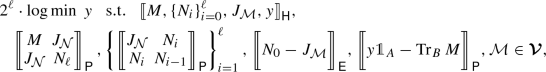 (19)
(19)where \(J_{{{{\mathcal {N}}}}}\) and \(J_{{{{\mathcal {M}}}}}\) are the corresponding Choi matrices of \({{{\mathcal {N}}}}\) and \({{{\mathcal {M}}}}\) respectively. Here the short notation that \(\llbracket X \rrbracket _{{\mathsf {P}}}\), \(\llbracket X \rrbracket _{{\mathsf {E}}}\) and \(\llbracket X \rrbracket _{{\mathsf {H}}}\) represent the positive semidefinite condition \(X \ge 0\), the equality condition \(X = 0\) and the Hermitian condition \(X = X^\dagger \), respectively.

Remark 2
Inequality (13) acts as a starting point of our improvement on the previous capacity bounds built on the max-relative entropy. The closed-form expression of the channel divergence directly leads to the additivity property in Item 3 and the semidefinite representation in Item 6. These properties should be contrasted with the situation for the Petz or sandwiched Rényi divergence for channels, for which it is unclear how they can be calculated efficiently. The chain rule is another fundamental property that sets a difference of the geometric Rényi divergence with other variants. Using the notion of amortized channel divergence [20]
the chain rule is equivalent to
That is, the “amortization collapse” for the geometric Rényi divergence. This solves an open question from [20, Eq. (55)] in the area of quantum channel discrimination.
Remark 3
Note that the properties in Item 3,4,5 do not hold for the Umegaki relative entropy in general unless we consider the regularized channel divergence [40]. This implies that these properties are not satisfied by the Petz or sandwiched channel Rényi divergences for \(\alpha \) in the neighbourhood of 1. As such, defining a measure with such desirable properties requires going away from the Umegaki relative entropy. We also note that it is unclear whether the Petz or sandwiched channel Rényi divergences are efficiently computable, let alone having a simple closed-form expression. These indicate that the results we obtained in this work based on the geometric Rényi divergence cannot be easily extended to the Umegaki relative entropy.
Remark 4
Except for the condition \({{{\mathcal {M}}}}\in \varvec{{{{\mathcal {V}}}}}\), the semidefinite representation in the above Item 6 with \(\alpha (\ell ) = 1 + 2^{-\ell }\) is described by \(\ell + 3\) linear matrix inequalities, each of size no larger than \(2d \times 2d\) with \(d = |A||B|\). Thus the computational complexity (time-usage) for computing \(\min _{{{{\mathcal {M}}}}\in \varvec{{{{\mathcal {V}}}}}} {{\widehat{D}}}_{\alpha }({{{\mathcal {N}}}}\Vert {{{\mathcal {M}}}})\) is the same as computing \(\min _{{{{\mathcal {M}}}}\in \varvec{{{{\mathcal {V}}}}}} D_{\max }({{{\mathcal {N}}}}\Vert {{{\mathcal {M}}}})\). In practice, taking \(\ell = 0\) (\(\alpha = 2\)) already gives an improved result and choosing \(\ell \) around \(8 - 10\) will make the separation more significant. Moreover, a slight modification can be done [14] to compute the optimization for any rational \(\alpha \in (1,2]\). But we will restrict our attention, without loss of generality, to the discrete values \(\alpha (\ell ) = 1 + 2^{-\ell }\) with \(\ell \in {{{\mathbb {N}}}}\).
3.2 Detailed proofs
In the following, we give a detailed proof of each property listed in Theorem 3.
Lemma 4
(Comparison with D and \(D_{\max }\)). For any quantum state \(\rho \), sub-normalized quantum state \(\sigma \) with \(\rho \ll \sigma \) and \(\alpha \in (1,2]\), the following relation holds
Proof
The first two inequalities follow from Eqs. (3) and (6). The third inequality follows since the geometric Rényi divergence is the largest Rényi divergence satisfying the data-processing inequality (see [15] or [35, Eq. (4.34)]). It remains to prove the last one. Since the geometric Rényi divergence is monotonically non-decreasing with respect to \(\alpha \),Footnote 4 it suffices to show that \({{\widehat{D}}}_2(\rho \Vert \sigma ) \le D_{\max }(\rho \Vert \sigma )\). This has been proved in [28, Remark 5.3.2]. We provide here a different proof by using their semidefinite representations. Recall that \(D_{\max }(\rho \Vert \sigma ) = \min \{\log t\,|\, \rho \le t \sigma \}\). Denote the optimal solution as t, and we have \(D_{\max }(\rho \Vert \sigma ) = \log t\) with \(0 \le \rho \le t \sigma \). Note that
where the last equality follows from the Schur complement characterization of the block positive semidefinite matrix. Take \(M = t \rho \), and we have
Thus \(M = t \rho \) is a feasible solution of optimization (23) which implies \({{\widehat{D}}}_2(\rho \Vert \sigma ) \le \log {\text {Tr}}[t \rho ] = \log t = D_{\max }(\rho \Vert \sigma )\). This completes the proof. \(\quad \square \)
Compared with \(D_{\max }\), it is clear that \({{\widehat{D}}}_\alpha \) gives a tighter approximation of the Umegaki relative entropy D from above. We provide a concrete example in Fig. 1 to give an intuitive understanding of the relations between different divergences.

Relations between Umegaki relative entropy D, Belavkin–Staszewski relative entropy \({{\widehat{D}}}\), max-relative entropy \(D_{\max }\), sandwiched Rényi divergence \({{\widetilde{D}}}_{\alpha }\), Petz Rényi divergence \({\overline{D}}_{\alpha }\) and geometric Rényi divergence \({{\widehat{D}}}_{\alpha }\)
Lemma 5
(Closed-form expression). For any quantum channel \({{{\mathcal {N}}}}_{A'\rightarrow B}\), subchannel \({{{\mathcal {M}}}}_{A'\rightarrow B}\) and \(\alpha \in (1,2]\), the geometric Rényi channel divergence is given by
where \(J_{AB}^{{{{\mathcal {N}}}}}\) and \(J_{AB}^{{{{\mathcal {M}}}}}\) are the corresponding Choi matrices of \({{{\mathcal {N}}}}\) and \({{{\mathcal {M}}}}\) respectively. Moreover, for the Belavkin–Staszewski channel divergence, its has the closed-form expression:
Proof
Note that for any quantum state \(\rho _{A}\) and its purification \(\phi _{AA'}\), we have the relation
By definition of the geometric Rényi divergence we have
where the third step follows from the transformer inequality given in Lemma 47 in Appendix A and the fact that we can assume by continuity that \(\rho _A\) has full rank.Footnote 5 The last line follows from the semidefinite representation of the infinity norm \(\Vert X\Vert _{\infty } = \max _{\rho \in {{{\mathcal {S}}}}} {\text {Tr}}X\rho \).
The expression for \({{\widehat{D}}}\) follows exactly the same steps by using Corollary 48 in Appendix A and replacing the weighted matrix geometric mean with the operator relative entropy. \(\quad \square \)
Lemma 6
(Additivity). Let \({{{\mathcal {N}}}}_1\) and \({{{\mathcal {N}}}}_2\) be two quantum channels and let \({{{\mathcal {M}}}}_1\) and \({{{\mathcal {M}}}}_2\) be two subchannels. Then for any \(\alpha \in (1,2]\) it holds that
Proof
Due to the closed-form expression in Lemma 5, we have
The first and last lines follow from Lemma 5. The second and third lines follow since the weighted matrix geometric mean and the infinity norm are multiplicative under tensor product. \(\quad \square \)
Lemma 7
(Chain rule). Let \(\rho \) be a quantum state on \({{{\mathcal {H}}}}_{RA}\), \(\sigma \) be a subnormalized state on \({{{\mathcal {H}}}}_{RA}\) and \({{{\mathcal {N}}}}_{A\rightarrow B}\) be a quantum channel, \({{{\mathcal {M}}}}_{A\rightarrow B}\) be a subchannel and \(\alpha \in (1,2]\). Then
Proof
Let \(|\Phi \rangle _{SA} = \sum _i |i\rangle _S|i\rangle _A\) be the unnormalized maximally entangled state. Denote \(J^{{{{\mathcal {N}}}}}_{SB}\) and \(J^{{{{\mathcal {M}}}}}_{SB}\) as the Choi matrices corresponding to \({{{\mathcal {N}}}}\) and \({{{\mathcal {M}}}}\), respectively. Then we have the identities (see e.g. [22, Eq.(11)])
For \(y = \Vert {\text {Tr}}_B\, G_{1-\alpha }(J_{SB}^{{{{\mathcal {N}}}}},J_{SB}^{{{{\mathcal {M}}}}})\Vert _\infty \), Lemma 5 ensures that
and by definition of the infinity norm we find
By definition of the geometric Rényi divergence and by using (40) we can write
where the first inequality follows from the transformer inequality given in Lemma 47 in Appendix A. The third line follows from the multiplicativity of weighted matrix geometric mean under tensor product. The second inequality uses (42) and the fact that \(X \mapsto {\text {Tr}}\, K X\) is monotone for positive operator K. Equation (48) follows from the identity \(\langle \Phi _{SA}| Y_{RA}\otimes {\mathbb {1}}_S|\Phi _{SA}\rangle = {\text {Tr}}_A\, Y_{RA}\). \(\quad \square \)
Lemma 8
(Sub-additivity). For any quantum channels \({{{\mathcal {N}}}}^1_{A\rightarrow B}\), \({{{\mathcal {N}}}}^2_{B\rightarrow C}\), any subchannels \({{{\mathcal {M}}}}^1_{A\rightarrow B}\), \({{{\mathcal {M}}}}^2_{B\rightarrow C}\) and \(\alpha \in (1,2]\), it holds
Proof
This is a direct consequence of the chain rule in Lemma 7. For any pure state \(\phi _{AR}\), we have
Taking a maximization of \(\phi _{AR}\) on the left hand side, we have the desired result. \(\quad \square \)
Lemma 9
(Semidefinite representation). Let \(\varvec{{{{\mathcal {V}}}}}\) be a set of subchannels from A to B characterized by certain semidefinite conditions. For any quantum channel \({{{\mathcal {N}}}}_{A\rightarrow B}\) and \(\alpha (\ell ) = 1+2^{-\ell }\) with \(\ell \in {{{\mathbb {N}}}}\), the optimization \(\min _{{{{\mathcal {M}}}}\in \varvec{{{{\mathcal {V}}}}}} {{\widehat{D}}}_{\alpha }({{{\mathcal {N}}}}\Vert {{{\mathcal {M}}}})\) can be computed by a semidefinite program:

where \(J_{{{{\mathcal {N}}}}}\) and \(J_{{{{\mathcal {M}}}}}\) are the corresponding Choi matrices of \({{{\mathcal {N}}}}\) and \({{{\mathcal {M}}}}\) respectively.
Proof
This is a direct consequence of the closed-form expression in Lemma 5 and the semidefinite representation of the weighted matrix geometric means in [14] (see also Lemma 46 in Appendix A), as well as the semidefinite representation of the infinity norm of an Hermitian operator \(\Vert X\Vert _\infty = \min \{y\,|\, X \le y{\mathbb {1}}\}\). \(\quad \square \)
4 Quantum Communication
4.1 Background
The quantum capacity of a noisy quantum channel is the maximum rate at which it can reliably transmit quantum information over asymptotically many uses of the channel. There are two different quantum capacities of major concern, the (unassisted) quantum capacity Q and the two-way assisted quantum capacity \(Q^{\leftrightarrow }\) , depending on whether classical communication is allowed between each channel uses.
The well-established quantum capacity theorem shows that the quantum capacity is equal to the regularized channel coherent information [5,6,7, 42,43,44],
where \(I_c({{{\mathcal {N}}}})\equiv \max _{\rho \in {{{\mathcal {S}}}}} \left[ H({{{\mathcal {N}}}}(\rho )) - H({{{\mathcal {N}}}}^c(\rho ))\right] \) is the channel coherent information, H is the von Neumann entropy and \({{{\mathcal {N}}}}^c\) is the complementary channel of \({{{\mathcal {N}}}}\). The regularization in (56) is necessary in general since the channel coherent information is non-additive [45, 46] and an unbounded number of channel uses may be required to detect capacity [47]. For this reason, the quantum capacity is notoriously difficult to evaluate, not to mention the scenario with two-way classical communication assistance.
Substantial efforts have been made in providing single-letter lower and upper bounds on Q and \(Q^{\leftrightarrow }\) (e.g. [48,49,50,51,52,53]). Most of them require certain symmetries of the channel to be computable or relatively tight. Of particular interest is a strong converse bound given by Tomamichel et al. [11]. Inspired by the Rains bound from entanglement theory [54], they introduced the Rains information (R) of a quantum channel and further proved that it is a strong converse rate for quantum communication through the channel. However, R is not known to be computable in general due to its minimax optimization of the Umegaki relative entropy. For the ease of computability, Wang et al. [21] relaxed the Umegaki relative entropy to the max-relative entropy, obtaining a variant known as the max-Rains information (\(R_{\max }\)). Leveraging the semidefinite representation of the max-relative entropy, they showed that \(R_{\max }\) is efficiently computable via a semidefinite program. It was later strengthened by Berta and Wilde [22] that \(R_{\max }\) is also a strong converse rate for quantum communication under two-way classical communication assistance. Since then, the max-Rains information \(R_{\max }\) is arguablyFootnote 6 the best-known computable strong converse bound on both assisted and unassisted quantum capacities in general.
4.2 Summary of results
In this part, we aim to improve the bound given by the max-Rains information in both assisted and unassisted scenarios. The structure of this part is organized as follows (see also a schematic diagram in Fig. 2).
In Sect. 4.3 we discuss the unassisted quantum communication. Based on the notion of the generalized Rains information in [11], we exhibit that the generalized Rains information induced by the geometric Rényi divergence (\({{\widehat{R}}}_{\alpha }\)) can be computed as a semidefinite program, improving the previously known result of the max-Rains information [21] in general. That is, we show that
where \(Q({{{\mathcal {N}}}})\) and \(Q^{\dagger }({{{\mathcal {N}}}})\) denote the unassisted quantum capacity of channel \({{{\mathcal {N}}}}\) and its corresponding strong converse capacity, respectively.
In Sect. 4.4, we study the quantum communication with PPT assistance, an assistance stronger than the two-way classical communication. We introduce the generalized Theta-information which is a new variant of channel information inspired by the channel resource theory (similar to the Upsilon-information in [57]). More precisely, we define the generalized Theta-information as a “channel distance” to the class of subchannels given by the zero set of Holevo–Werner bound (\(Q_{\Theta }\)) [48]. Interestingly, we show that the max-Rains information \(R_{\max }\) coincides with the generalized Theta-information induced by the max-relative entropy \(R_{\max ,\Theta }\), i.e., \(R_{\max } = R_{\max ,\Theta }\), thus providing a completely new perspective of understanding the former quantity. Moreover, we prove that the generalized Theta-information induced by the geometric Rényi divergence (\({{\widehat{R}}}_{\alpha ,\Theta }\)) is a strong converse bound on the PPT-assisted quantum capacity by utilizing an “amortization argument”. Together with its SDP formula, we conclude that \({{\widehat{R}}}_{\alpha ,\Theta }\) improves the previous result of the max-Rains information [22] in general. That is, we show that
where \(Q^{{{\mathrm{PPT}}},\leftrightarrow }({{{\mathcal {N}}}})\) and \(Q^{{{\mathrm{PPT}}},\leftrightarrow ,\dagger }({{{\mathcal {N}}}})\) denote the PPT-assisted quantum capacity of channel \({{{\mathcal {N}}}}\) and its corresponding strong converse capacity, respectively.
In Sect. 4.5, we consider the PPT-assisted quantum communication via bidirectional quantum channels, a more general model than the usual point-to-point channels. We extend the results in Sect. 4.4 to this general model and demonstrate an improvement to the previous result of the bidirectional max-Rains information (\(R_{\max }^{{\mathrm{bi}}}\)) [23]. That is, we show that
where \(Q^{{\mathrm{bi}},{{\mathrm{PPT}}},\leftrightarrow }({{{\mathcal {N}}}})\) and \(Q^{{\mathrm{bi}},{{\mathrm{PPT}}},\leftrightarrow ,\dagger }({{{\mathcal {N}}}})\) denote the PPT-assisted quantum capacity of a bidirectional channel \({{{\mathcal {N}}}}\) and its corresponding strong converse capacity, respectively.
Finally in Sect. 4.6 we investigate several fundamental quantum channels, demonstrating the efficiency of our new strong converse bounds. It turns out that our new bounds work exceptionally well and exhibit a significant improvement on the max-Rains information for almost all cases.

Relations between different converse bounds for quantum communication. \(Q^*\) and \(Q^{*,\dagger }\) are the quantum capacity with assistance \(*\) and its corresponding strong converse capacity, respectively. R, \({{\widehat{R}}}_\alpha \) and \(R_{\max }\) are the generalized Rains information induced by different quantum divergences. \({{\widehat{R}}}_{\alpha ,\Theta }\) and \(R_{\max ,\Theta }\) are the generalized Theta-information induced by different quantum divergences. \(Q_\Theta \) is the Holevo–Werner bound. The circled quantities are those of particular interest in quantum information theory. The key quantities and the main contributions in this part are marked in red. The quantity at the start point of an arrow is no smaller than the one at the endpoint. The double arrow represents that two quantities coincide. The inequality sign represents that two quantities are not the same in general. The dotted arrow represents that the relation holds under certain restrictions, where “cov.” stands for “covariant”. The parameter \(\alpha \) is taken in the interval (1, 2]. The quantities in the shaded area are SDP computable in general
4.3 Unassisted quantum capacity
In this section, we discuss converse bounds on the unassisted quantum capacity.Footnote 7
Definition 10
([11]). For any generalized divergence \({\varvec{D}}\), the generalized Rains bound of a quantum state \(\rho _{AB}\) is defined as
where the minimization is taken over the Rains set \({{\mathrm{PPT}}}'(A:B) \equiv \big \{\sigma _{AB}\,\big |\, \sigma _{AB} \ge 0,\,\big \Vert \sigma _{AB}^{{\mathsf {T}}_B}\big \Vert _1 \le 1\big \}\).
Definition 11
([11]). For any generalized divergence \({\varvec{D}}\), the generalized Rains information of a quantum channel \({{{\mathcal {N}}}}_{A'\rightarrow B}\) is defined as
where \(\phi _{AA'}\) is a purification of quantum state \(\rho _A\).
In particular, the Rains information is induced by the Umegaki relative entropy [11],
The max-Rains information is induced by the max-relative entropy [21],
Denote \({{\widehat{R}}}_{\alpha }\) as the generalized Rains information induced by the geometric Rényi divergence. We have the following result.
Theorem 12
(Application 1). For any quantum channel \({{{\mathcal {N}}}}\) and \(\alpha \in (1,2]\), it holds
where \(Q({{{\mathcal {N}}}})\) and \(Q^{\dagger }({{{\mathcal {N}}}})\) denote the unassisted quantum capacity of channel \({{{\mathcal {N}}}}\) and its corresponding strong converse capacity, respectively.
Proof
The first two inequalities follow since the Rains information \(R({{{\mathcal {N}}}})\) has been proved to be a strong converse bound on the unassisted quantum capacity [11]. The last two inequalities are direct consequences of the inequalities in Lemma 4. \(\quad \square \)
Remark 5
Note that in the limit of \(\alpha \rightarrow 1\), the bound \({{\widehat{R}}}_{\alpha }\) will converge to the Rains information induced by the Belavkin–Staszewski relative entropy due to Eq. (11).
The following result shows how to compute the newly introduced bound \({{\widehat{R}}}_{\alpha }({{{\mathcal {N}}}})\) as an SDP.
Proposition 13
(SDP formula). For any quantum channel \({{{\mathcal {N}}}}\) and \(\alpha (\ell ) = 1+2^{-\ell }\) with \(\ell \in {\mathbb {N}}\), it holds
with \(S_\alpha ({{{\mathcal {N}}}})\) given by the following SDP

where \(J_{{{{\mathcal {N}}}}}\) is the Choi matrix of \({{{\mathcal {N}}}}\) and \(X^{{\mathsf {H}}} \equiv X + X^\dagger \) denotes the Hermitian part of X.
Proof
The proof involves a non-trivial scaling technique for variables replacement, which is important for simplifying the minimax optimization of \({{\widehat{R}}}_{\alpha }\) to a single SDP. More formally, this proof contains two steps. First we derive a suitable SDP formula for \({{\widehat{R}}}_\alpha (\rho _{AB})\) in terms of a maximization problem. Second, we replace \(\rho _{AB}\) as the channel’s output state \({{{\mathcal {N}}}}_{A'\rightarrow B}(\phi _{AA'})\) and maximize over all the input state \(\rho _A\). Since the SDP maximization formula for \({{\widehat{R}}}_\alpha (\rho _{AB})\) is not necessarily unique, we need to find a suitable one which is able to give us an overall semidefinite optimization in the second step.
Step One: Combining the semidefinite representation of the geometric Rényi divergence in Lemma 46 and the semidefinite representation of the Rains set \({{\mathrm{PPT}}}'(A:B)=\big \{\sigma _{AB}\ge 0 \,|\, \sigma _{AB}^{{\mathsf {T}}_{ B}} = X_{AB} - Y_{AB},\, {\text {Tr}}(X_{AB} + Y_{AB}) \le 1,\, X_{AB} \ge 0,\, Y_{AB} \ge 0\big \}\), we have the SDP formula for the geometric Rényi Rains bound as,

By the Lagrange multiplier method, the dual SDP is given by

Due to the Slater’s condition, we can easily check that the strong duality holds. Note that both (64) and (65) are already SDPs for any quantum state \(\rho _{AB}\). However, the last condition in (65) will introduce a non-linear term if we perform the second step of proof at this stage. The following trick will help us get rid of the variable f which is essential to obtain the final result. Note that the last condition above implies \(f \ge 0\) and together with the rest conditions we necessarily have \(f > 0\). Replacing the variables as
we obtain an equivalent SDP of \({{\widehat{R}}}_{\alpha }(\rho _{AB})\) as

Denote the objective function \(f^{{1}/({2^\ell + 1})} \cdot a - f\) with \(a = {\text {Tr}}\big [\big ({{\widetilde{K}}}^{{\mathsf {H}}} - \sum _{i=1}^\ell {{\widetilde{W}}}_i \big )\varvec{\cdot }\rho \big ] \ge 0\). For any fixed value a, the optimal solution is taken at \(f = [{a}/({2^\ell +1})]^{1+1/2^\ell }\) with the maximal value \(2^\ell [{a}/({2^\ell + 1})]^{1+1/2^\ell }\). Without loss of generality, we can replace the objective function with \(2^\ell [{a}/({2^\ell + 1})]^{1+1/2^\ell }\) and get rid of the variable f. Direct calculation gives us

Step Two: Note that \({{{\mathcal {N}}}}_{A'\rightarrow B}(\phi _{AA'}) = \sqrt{\rho _A} J_{{{{\mathcal {N}}}}} \sqrt{\rho _A}\) holds for any quantum state \(\rho _A\) with purification \(\phi _{AA'}\). Thus the final result is straightforward from (68) by replacing the input state \(\rho _{AB}\) as \(\sqrt{\rho _A} J_{{{{\mathcal {N}}}}} \sqrt{\rho _A}\), replacing \(K,Z_i,W_i\) as \(\rho _A^{-1/2} K \rho _A^{-1/2},\rho _A^{-1/2} Z_i \rho _A^{-1/2}, \rho _A^{-1/2} W_i\rho _A^{-1/2}\) respectively and maximizing over all input state \(\rho _A\). \(\quad \square \)
4.4 Two-way assisted quantum capacity
In this section, we discuss converse bounds on two-way assisted quantum capacity.Footnote 8 Recall that the Rains bound in (57) is essentially established as the divergence between the given state and the Rains set—a set of sub-normalized states given by the zero setFootnote 9 of the log-negativity \(E_N(\rho _{AB})\equiv \log \Vert \rho _{AB}^{{\mathsf {T}}_B}\Vert _1\) [58]. With this in mind, we introduce a new variant of the channel’s analog of Rains bound, compatible with the notion of channel resource theory. Specifically, consider the Holevo–Werner bound [48]—a channel’s analog of the log-negativity,
where \(\Theta \) is the transpose map and \(\Vert {{{\mathcal {F}}}}_{A'\rightarrow B}\Vert _\diamondsuit \equiv \sup _{X_{AA'}\in {{{\mathcal {L}}}}(AA')} \Vert {{{\mathcal {F}}}}_{A'\rightarrow B}(X_{AA'})\Vert _1/ \Vert X_{AA'}\Vert _1\) is the diamond norm [59]. In particular, this bound can be represented as the following SDP,
Inspired by the formulation of the Rains set, we define the set of subchannels given by the zero set of the Holevo–Werner bound \(Q_{\Theta }\) as
Definition 14
(Theta-info.). For any generalized divergence \({\varvec{D}}\), the generalized Theta-informationFootnote 10 of a quantum channel \({{{\mathcal {N}}}}_{A'\rightarrow B}\) is defined as
where \({\varvec{{{{\mathcal {V}}}}}_\Theta }\) is the Theta set in (71) and \(\phi _{AA'}\) is a purification of quantum state \(\rho _A\).
Remark 6
On the r.h.s. of Eq. (72), the objective function is concave in \(\rho _A\) and convex in \({{{\mathcal {M}}}}\) [57, Proposition 8]. Thus we can swap the min and max by using Sion’s minimax theorem [60].
The following result compares the generalized Theta-information in (72) and the generalized Rains information in (58) presented in the previous section. Interestingly, these two quantities coincide for the max-relative entropy in general.
Proposition 15
For any generalized divergence \({\varvec{D}}\) and any quantum channel \({{{\mathcal {N}}}}\), it holds
Moreover, for the max-relative entropy the equality always holds, i.e,
Proof
We prove the relation (73) first. Note that for any pure state \(\phi _{AA'}\) and \({{{\mathcal {M}}}}_{A'\rightarrow B} \in \varvec{{{{\mathcal {V}}}}}_\Theta \), we have
This implies \({{{\mathcal {M}}}}_{A'\rightarrow B}(\phi _{AA'}) \in {{\mathrm{PPT}}}'(A:B)\). Then it holds
The first and last line follow by definition. The inequality holds since \({{{\mathcal {M}}}}_{A'\rightarrow B}(\phi _{AA'}) \in {{\mathrm{PPT}}}'(A:B)\) and thus the first line is minimizing over a larger set. In the third line, we swap the min and max by the argument in Remark 6.
We next prove the Eq. (74). Recall that the SDP formula of the max-Rains information is given by ([21, Proposition 5] or [61, Eq. (11)])
Replace V and Y with \(\mu V\) and \(\mu Y\) respectively, and then denote \(N = (V- Y)^{{\mathsf {T}}_B}\), we have
Notice that the second to the last conditions define a set of CP maps
Combining (81) and (82), we obtain \(R_{\max }({{{\mathcal {N}}}}) = \min _{{{{\mathcal {M}}}}\in \varvec{{{{\mathcal {V}}}}}} D_{\max }({{{\mathcal {N}}}}\Vert {{{\mathcal {M}}}})\). Thus it suffices for us to show the equivalence \(\varvec{{{{\mathcal {V}}}}}= \varvec{{{{\mathcal {V}}}}}_\Theta \). For any \({{{\mathcal {M}}}}\in \varvec{{{{\mathcal {V}}}}}_\Theta \), take \(V = (R + J_{{{{\mathcal {M}}}}}^{{\mathsf {T}}_B})/2\) and \(Y = (R - J_{{{{\mathcal {M}}}}}^{{\mathsf {T}}_B})/2\). Then \(V \ge 0\), \(Y \ge 0\), \(J_{{{{\mathcal {M}}}}}^{{\mathsf {T}}_B} = V-Y\) and \({\text {Tr}}_B (V+Y) = {\text {Tr}}_B R \le {\mathbb {1}}_A\), which implies \({{{\mathcal {M}}}}\in \varvec{{{{\mathcal {V}}}}}\). On the other hand, for any \({{{\mathcal {M}}}}\in \varvec{{{{\mathcal {V}}}}}\), take \(R = V + Y\). We can check that \({\text {Tr}}_B R = {\text {Tr}}_B(V+Y) \le {\mathbb {1}}_A\), \(R + J_{{{{\mathcal {M}}}}}^{{\mathsf {T}}_B} = (V+Y) + (V-Y) = 2V \ge 0\) and \(R - J_{{{{\mathcal {M}}}}}^{{\mathsf {T}}_B} = (V+Y) - (V-Y) = 2Y \ge 0\), which implies \({{{\mathcal {M}}}}\in \varvec{{{{\mathcal {V}}}}}_\Theta \). Finally we have
which completes the proof. \(\quad \square \)
We proceed to consider the geometric Rényi divergence and show its amortization property, a key ingredient to proving the strong converse bound on the assisted quantum capacity in Theorem 17.
Suppose Alice and Bob share a quantum state \(\rho _{A'AB'}\) with the system cut \(A'A:B'\). Their shared entanglement with respect to the measure \({{\widehat{R}}}_\alpha \) is given by \({{\widehat{R}}}_\alpha (\rho _{A'A:B'})\). If Alice redistributes part of her system A through the channel \({{{\mathcal {N}}}}_{A\rightarrow B}\) and Bob receives the output system B, then their shared state becomes to \(\omega _{A':BB'} = {{{\mathcal {N}}}}_{A\rightarrow B}(\rho _{A'A:B'})\) with the shared entanglement evaluated as \({{\widehat{R}}}_\alpha (\omega _{A':BB'})\). The amortization inequality shows that the amount of entanglement change after the state redistribution is upper bounded by the channel’s information measure \({{\widehat{R}}}_{\alpha ,\Theta }({{{\mathcal {N}}}})\).
Proposition 16
(Amortization). For any quantum state \(\rho _{A'AB'}\), any quantum channel \({{{\mathcal {N}}}}_{A\rightarrow B}\) and the parameter \(\alpha \in (1,2]\), it holds
Proof
This is a direct consequence of the chain rule property of the geometric Rényi divergence in Lemma 7. Suppose the optimal solutions of \({{\widehat{R}}}_\alpha (\rho _{A'A:B'})\) and \({{\widehat{R}}}_{\alpha ,\Theta }({{{\mathcal {N}}}}_{A\rightarrow B})\) are taken at \(\sigma _{A'AB'}\in {{\mathrm{PPT}}}'(A'A:B')\) and \({{{\mathcal {M}}}}\in \varvec{{{{\mathcal {V}}}}}_{\Theta }\), respectively. Let \( \gamma _{A'BB'} = {{{\mathcal {M}}}}_{A\rightarrow B}(\sigma _{A'AB'})\). We have
where the first inequality follows from the definition of diamond norm and the second inequality follows from the choice of \(\sigma _{A'AB'}\) and \({{{\mathcal {M}}}}_{A\rightarrow B}\). Thus \(\gamma _{A'BB'} \in {{\mathrm{PPT}}}'(A':BB')\) and forms a feasible solution for \({{\widehat{R}}}_\alpha (\omega _{A':BB'})\). Then we have
The second inequality follows from the chain rule of the geometric Rényi divergence in Lemma 7, and the last line follows by the optimality assumption of \({{{\mathcal {M}}}}\) and \(\sigma \). \(\quad \square \)

A schematic diagram for the protocol of \({{{\mathcal {O}}}}\)-assisted quantum communication that uses a quantum channel n times, where \({{{\mathcal {O}}}}\) is usually chosen as \({{\mathrm{LOCC}}}\) or \({{\mathrm{PPT}}}\). Every channel use is interleaved by an operation in the class \({{{\mathcal {O}}}}\). The goal of such a protocol is to produce an approximate maximally entangled state \(\omega _{M_A M_B}\) between Alice and Bob. The systems in red are held by Alice while the systems in blue are held by Bob
Theorem 17
(Application 2). For any quantum channel \({{{\mathcal {N}}}}\) and \(\alpha \in (1,2]\), it holds
where \(Q^{{{\mathrm{PPT}}},\leftrightarrow }({{{\mathcal {N}}}})\) and \(Q^{{{\mathrm{PPT}}},\leftrightarrow ,\dagger }({{{\mathcal {N}}}})\) denote the PPT-assisted quantum capacity of channel \({{{\mathcal {N}}}}\) and its corresponding strong converse capacity, respectively.
Proof
The first inequality holds by definition. The last inequality holds since we have \( {{\widehat{R}}}_{\alpha ,\Theta }({{{\mathcal {N}}}}) \le R_{\max ,\Theta }({{{\mathcal {N}}}}) = R_{\max }({{{\mathcal {N}}}})\) by Lemma 4 and Proposition 15, respectively. It remains to prove the second one. Once we have the amortization inequality in Proposition 16, the proof of the second inequality will closely follow the one in [22, Theorem 3]. Consider n round PPT-assisted quantum communication protocol illustrated in Fig. 3. For the i-th round, denote the input state of \({{{\mathcal {N}}}}\) as \(\rho _{A'AB'}^{\scriptscriptstyle (i)}\) and the output state as \(\sigma _{A'BB'}^{\scriptscriptstyle (i)}\). The final state after n rounds communication is denoted as \(\omega _{M_AM_B}\). Then we have
The first and third lines follow from the monotonicity of the geometric Rényi Rains bound \({{\widehat{R}}}_\alpha \) with respect to the PPT operations [11, Eq. (22)]. The second line follows since \(\rho _{A'A:B'}^{\scriptscriptstyle (1)}\) is a PPT state and thus \({{\widehat{R}}}_{\alpha }(\rho ^{\scriptscriptstyle (1)}_{A'A:B'}) = 0\). The last line follows from Proposition 16.
Note that any communication protocol is characterized by a triplet \((n,r,\varepsilon )\) with the number of rounds n, the communication rate r, and the error tolerance \(\varepsilon \). Denote \(k \equiv 2^{nr}\) and we have \({\text {Tr}}\Phi _k \,\omega \ge 1-\varepsilon \) with \(\Phi _k\) being the k-dimensional maximally entangled state. Moreover, for any \(\sigma \in {{\mathrm{PPT}}}'\), it holds \({\text {Tr}}\Phi _k \sigma \le 1/k\) [54]. Without loss of generality, we can assume that \(\varepsilon \le 1-2^{-nr}\). Otherwise, any rate above the capacity would satisfy the strong converse property since \(1-\varepsilon < 2^{-nr}\). Thus for any \(\sigma \in {{\mathrm{PPT}}}'\) we have
Let \({{{\mathcal {N}}}}(\gamma ) = ({\text {Tr}}\Phi _k \gamma ) |0\rangle \langle 0| + ({\text {Tr}}({\mathbb {1}}-\Phi _k) \gamma ) |1\rangle \langle 1|\). Due to the data-processing inequality, we have
where \(\delta _\alpha (p\Vert q)\equiv \frac{1}{\alpha -1} \log \big [p^\alpha q^{1-\alpha } + (1-p)^\alpha (1-q)^{1-\alpha }\big ]\) is the binary classical Rényi divergence. The last inequality in (97) follows from the monotonicity property that \(\delta _\alpha (p'\Vert q) \le \delta _\alpha (p\Vert q)\) if \(p \le p' \le q\) and \(\delta _\alpha (p\Vert q') \le \delta _\alpha (p\Vert q)\) if \(p \le q' \le q\) [62]. Then we have
Combining Eqs. (91) and (98), we have
which is equivalent to
This implies that if the communication rate r is strictly larger than \({{\widehat{R}}}_{\alpha ,\Theta }({{{\mathcal {N}}}})\), the fidelity of transmission \(1-\varepsilon \) decays exponentially fast to zero as the number of channel use n increases. Or equivalently, we have the strong converse inequality \(Q^{{{\mathrm{PPT}}},\leftrightarrow ,\dagger }({{{\mathcal {N}}}}) \le {{\widehat{R}}}_{\alpha ,\Theta }({{{\mathcal {N}}}}) \) and completes the proof. \(\quad \square \)
Let \(Q^{\leftrightarrow }\) and \(Q^{\leftrightarrow ,\dagger }\) be the two-way assisted quantum capacity and its strong converse capacity respectively. We have the following as a direct consequence of Theorem 17, since PPT assistance is stronger.
Corollary 18
For any quantum channel \({{{\mathcal {N}}}}\) and \(\alpha \in (1,2]\), it holds
Finally, we present how to compute \({{\widehat{R}}}_{\alpha ,\Theta }({{{\mathcal {N}}}})\) as an SDP.
Proposition 19
(SDP formula). For any quantum channel \({{{\mathcal {N}}}}_{A'\rightarrow B}\) and \(\alpha (\ell ) = 1+2^{-\ell }\) with \(\ell \in {\mathbb {N}}\), the geometric Rényi Theta-information can be computed as an SDP:

where \(J_{{{{\mathcal {N}}}}}\) is the Choi matrix of \({{{\mathcal {N}}}}\).
Proof
This directly follows from Lemma 9 and the definition of the Theta set \(\varvec{{{{\mathcal {V}}}}}_\Theta \) in (71). \(\quad \square \)
4.5 Extension to bidirectional channels
In this section we showcase that the above results for the PPT/two-way assisted quantum capacity can be extended to a more general scenario where Alice and Bob share a bidirectional quantum channel.
A bipartite quantum channel \({{{\mathcal {N}}}}_{A_1B_1\rightarrow A_2B_2}\) is a completely positive trace-preserving map that sends composite system \(A_1B_1\) to \(A_2B_2\). This channel is called bidirectional channel if \(A_1A_2\) are held by Alice and \(B_1B_2\) are held by Bob. That is, Alice and Bob each input a state to this channel and receive an output [63], as depicited in Fig. 4. This is the most general setting for two-party communications and will reduce to the usual point-to-point channel when the dimensions of Bob’s input and Alice’s output are trivial, i.e., \(\dim ({{{\mathcal {H}}}}_{B_1}) = \dim ({{{\mathcal {H}}}}_{A_2}) = 1\).

A model of bidirectional quantum channel where \(A_1\), \(A_2\) are held by Alice and \(B_1\), \(B_2\) by Bob
In [23], the authors introduced the bidirectional version of the max-Rains information as
Let \(Q^{{\mathrm{bi}},{{\mathrm{PPT}}},\leftrightarrow }\) and \(Q^{{\mathrm{bi}},{{\mathrm{PPT}}},\leftrightarrow ,\dagger }\) be the PPT-assisted quantum capacity of a bidirectional channel and its strong converse capacity respectively.Footnote 11 It was proved in [23] that
Following a similar approach in Sect. 4.4, we can further strengthen this bound by exploiting the geometric Rényi divergence.
We start with a bidirectional version of the Werner–Holevo boundFootnote 12
and define its zero set \(\varvec{{{{\mathcal {V}}}}}^{\mathrm{bi}}_{\Theta }\) which admits a semidefinite representation as
Using the same idea as the point-to-point scenario, we defined the generalized Theta-information of a bidirectional channel \({{{\mathcal {N}}}}_{A_1B_1\rightarrow A_2 B_2}\) as the “channel distance”Footnote 13
where \({\varvec{D}}\) is a generalized divergence and the channel divergence follows from the usual definition
by maximizing over all the pure states \(\phi _{A_1B_1A_3B_3}\).
Following a similar proof of Proposition 15, we can show that the bidirectional max-Rains information defined in (106) coincides with the bidirectional Theta-information induced by the max-relative entropy. That is,
Denote the bidirectional Rains bound as \({{\widehat{R}}}_{\alpha }^{{\mathrm{bi}}}(\rho ) \equiv \min _{\sigma \ge 0, \Vert \sigma ^{{\mathsf {T}}_{B_1B_2}}\Vert _1 \le 1} {{\widehat{D}}}_{\alpha }(\rho \Vert \sigma )\). A similar proof as Proposition 16 gives us the following amortization inequality.
Proposition 20
(Amortization). For any quantum state \(\rho _{A_1A_3:B_1B_3}\), any bidirectional quantum channel \({{{\mathcal {N}}}}_{A_1B_1\rightarrow A_2B_2}\) and \(\alpha \in (1,2]\), it holds
with the output state \(\omega _{A_2A_3:B_2B_3} = {{{\mathcal {N}}}}_{A_1B_1\rightarrow A_2B_2}(\rho _{A_1A_3:B_1B_3})\).
Using the amortization inequality in Proposition 20 and a standard argument as Theorem 17, we have the analog results of Theorem 17 and Corollary 18 for bidirectional channels as follows:
Theorem 21
(Main result 3). For any bidirectional channel \({{{\mathcal {N}}}}_{A_1B_1\rightarrow A_2B_2}\) and \(\alpha \in (1,2]\), it holds
where \(Q^{{\mathrm{bi}},{{\mathrm{PPT}}},\leftrightarrow }({{{\mathcal {N}}}})\) and \(Q^{{\mathrm{bi}},{{\mathrm{PPT}}},\leftrightarrow ,\dagger }({{{\mathcal {N}}}})\) denote the PPT-assisted quantum capacity of a bidirectional channel \({{{\mathcal {N}}}}\) and its corresponding strong converse capacity, respectively. As a consequence, it holds
where \(Q^{{\mathrm{bi}},\leftrightarrow }({{{\mathcal {N}}}})\) and \(Q^{{\mathrm{bi}},\leftrightarrow ,\dagger }({{{\mathcal {N}}}})\) denote the two-way assisted quantum capacity of a bidirectional channel \({{{\mathcal {N}}}}\) and its corresponding strong converse capacity, respectively.
Proposition 22
(SDP formula). For any bidirectional channel \({{{\mathcal {N}}}}_{A_1B_1\rightarrow A_2B_2}\) and \(\alpha (\ell ) = 1+2^{-\ell }\) with \(\ell \in {{{\mathbb {N}}}}\), the bidirectional geometric Rényi Theta-information can be computed as an SDP:

where \(J_{{{{\mathcal {N}}}}}\) is the Choi matrix of \({{{\mathcal {N}}}}\).
Proof
This directly follows from Lemma 9 and the definition of \(\varvec{{{{\mathcal {V}}}}}^{\mathrm{bi}}_{\Theta }\) in (109). \(\quad \square \)
4.6 Examples
In this section, we investigate several fundamental quantum channels as well as their compositions. We use these toy models to test the performance of our new strong converse bounds, demonstrating the improvement on the previous results. The semidefinite programs are implemented in MATLAB via the CVX package [66, 67], by the solver “Mosek” [68] with the best precision.Footnote 14
4.6.1 Fundamental quantum channels
The quantum depolarizing channel with dimension d is defined as
The quantum erasure channel is defined as
where \(|e\rangle \) is an erasure state orthogonal to the input Hilbert space. The quantum dephasing channel is defined as
where \(Z = |0\rangle \langle 0| - |1\rangle \langle 1|\) is the Pauli-z operator. These three classes of channels are covariant with respect to the whole unitary group. The generalized amplitude damping (GAD) channel is defined as
with the Kraus operators
The GAD channel is one of the realistic sources of noise in superconducting-circuit-based quantum computing [69], which can viewed as the qubit analogue of the bosonic thermal channel. When \(N = 0\), it reduces to the conventional amplitude damping channel with two Kraus operators \(A_1\), \(A_2\).
4.6.2 Comparison for the unassisted quantum capacity
For the unassisted quantum capacity, we compare the qubit depolarizing channel \({{{\mathcal {D}}}}_p\), the qubit erasure channel \({{{\mathcal {E}}}}_p\), the qubit dephasing channel \({{{\mathcal {Z}}}}_p\) and the generalized amplitude damping channels \({{{\mathcal {A}}}}_{p,N}\) with different choices of parameter N.
Since \({{{\mathcal {D}}}}_p\), \({{{\mathcal {E}}}}_p\) and \({{{\mathcal {Z}}}}_p\) are covariant with respect to the unitary group, the optimal input state \(\rho _A\) of their Rains information is taken at the maximally mixed state [11, Proposition 2]. Therefore, their Rains information can be computed via the algorithm in [55, 56]. Moreover, for any parameters \(\gamma ,N \in [0,1]\), the GAD channel \({{{\mathcal {A}}}}_{\gamma ,N}\) is covariant with respect to the Pauli-z operator Z. That is, \({{{\mathcal {A}}}}_{\gamma ,N}(Z\rho Z) = Z {{{\mathcal {A}}}}_{\gamma ,N}(\rho )Z\) for all quantum state \(\rho \). To compute its Rains information, it suffices to perform the maximization over input states with respect to the one-parameter family of states \(\rho _A = (1-p)|0\rangle \langle 0| + p |1\rangle \langle 1|\) [70]. This can be handled, for example, by MATLAB function “fminbnd”.
The comparison results are shown in Fig. 5. It is clear that the geometric Rényi Rains information \({{\widehat{R}}}_{\alpha {\scriptscriptstyle (10)}}\) coincide with the Rains information R for all these channels except for the particular case \({{{\mathcal {A}}}}_{p,0}\) in subfigure (d). For all cases, \({{\widehat{R}}}_{\alpha {\scriptscriptstyle (10)}}\) sets a big difference from the max-Rains information \(R_{\max }\).

Comparison of the strong converse bounds on the unassisted quantum capacity of the qubit depolarizing channel \({{{\mathcal {D}}}}_p\), the qubit erasure channel \({{{\mathcal {E}}}}_p\), the qubit dephasing channel \({{{\mathcal {Z}}}}_p\) and the generalized amplitude damping channels \({{{\mathcal {A}}}}_{p,N}\). The horizontal axis takes value of \(p \in [0,1]\) and the parameter \(\alpha (10) = 1+2^{-10}\)
4.6.3 Comparison for the two-way assisted quantum capacity
For the two-way assisted quantum capacity, we consider the channels \({{{\mathcal {D}}}}_p\), \({{{\mathcal {E}}}}_p\) and \({{{\mathcal {Z}}}}_p\) composed with the amplitude damping channel \({{{\mathcal {A}}}}_{p,0}\), and the generalized amplitude damping channel \({{{\mathcal {A}}}}_{p,N}\) with different choices of parameter N. Because these channels are not covariant w.r.t. the whole unitary group, their Rains information are not known as valid converse bounds on the two-way assisted quantum capacity.
The comparison resultFootnote 15 for the two-way assisted quantum capacity is given in Fig. 6. The geometric Rényi Theta-information \({{\widehat{R}}}_{\alpha {\scriptscriptstyle (10)},\Theta }\) demonstrates a significant improvement over the max-Rains information \(R_{\max }\) for all these channels except for one particular case \({{{\mathcal {A}}}}_{p,0}\) in subfigure (d).

Comparison of the strong converse bounds on the two-way assisted quantum capacity of the channels \({{{\mathcal {D}}}}_p\), \({{{\mathcal {E}}}}_p\) and \({{{\mathcal {Z}}}}_p\) composed with the amplitude damping channel \({{{\mathcal {A}}}}_{p,0}\), and the generalized amplitude damping channels \({{{\mathcal {A}}}}_{p,N}\) with different parameters. The horizontal axis takes value of \(p \in [0,1]\) and the parameter \(\alpha (10) = 1+2^{-10}\)
4.6.4 Comparison for the two-way assisted quantum capacity of bidirectional channels
Consider a typical noise in a quantum computer which is modeled as [23]
where S is the swap operator and \(U_\phi = |00\rangle \langle 00| + e^{i\phi } |01\rangle \langle 01| + e^{i\phi } |10\rangle \langle 10| + e^{2i\phi } |11\rangle \langle 11|\) is the collective dephasing noise. The comparison result of our new bound \({{\widehat{R}}}^{\mathrm{bi}}_{\alpha {\scriptscriptstyle (10)},\Theta }\) with the previous bound \(R^{\mathrm{bi}}_{\max }\) is given in Fig. 7.

Comparison of the strong converse bounds on the two-way assisted quantum capacity of the bidirectional channels in (123) with the dephasing parameter choosing from \(\phi \in \{\pi , \pi /2,\pi /3\}\). The horizontal axis takes value of \(p \in [0,1]\) and the parameter \(\alpha (10) = 1+2^{-10}\)
5 Private Communication
5.1 Background
The private capacity of a quantum channel is defined as the maximum rate at which classical information can be transmitted privately from the sender (Alice) to the receiver (Bob). By “private”, it means a third party (Eve) who has access to the channel environment cannot learn anything about the information that Alice sends to Bob. There are also two different private capacities of major concern, the (unassisted) private capacity P and the two-way assisted private capacity \(P^{\leftrightarrow }\), depending on whether classical communication is allowed between each channel uses.
In the same spirit of the quantum capacity theorem, the private capacity theorem states that the private capacity of a quantum channel is given by its regularized private information [7, 71],
where \(I_p({{{\mathcal {N}}}}) \equiv \max _{{\mathscr {E}}} \left[ \chi ({\mathscr {E}}, {{{\mathcal {N}}}}) - \chi ({\mathscr {E}}, {{{\mathcal {N}}}}^c)\right] \) is the private information with the maximization taken over all quantum state ensembles \({\mathscr {E}} = \{p_i, \rho _i\}\), \(\chi ({\mathscr {E}}, {{{\mathcal {N}}}}) \equiv H(\sum _i p_i {{{\mathcal {N}}}}(\rho _i)) - \sum _i p_i H({{{\mathcal {N}}}}(\rho _i))\) is the Holevo information of the ensemble \({\mathscr {E}}\), H is the von Neumann entropy and \({{{\mathcal {N}}}}^c\) is the complementary channel of \({{{\mathcal {N}}}}\). The regularization in (124) is necessary in general since the private information is proved to be non-additive [72] and an unbounded number of channel uses may be required to achieve its private capacity [73].
Despite their importance in understanding the fundamental limits of quantum key distributions [74], much less is known about the converse bounds on private capacities, mostly due to their inherently involved settings. The squashed entanglement of a channel was proposed in [75] and proved to be a converse bound on the two-way assisted private capacity. But it remains unknown to be a strong converse rate and the quantity itself is difficult to compute exactly [8]. The entanglement cost of a channel was introduced in [76] and shown to be a strong converse bound on the two-way assisted private capacity [25]. But it was not given by a single-letter formula. A closely related quantity to this part is the relative entropy of entanglement of a channel (\(E_R\)), which was proved as a (weak) converse bound on the two-way assisted private capacity for channels with “covariant symmetry” [24]. This was later strengthened in [12] as a strong converse bound on the unassisted private capacity for general quantum channels and a strong converse bound on the two-way assisted private capacity for channels with “covariant symmetry”. Moreover, the max-relative entropy of entanglement of a channel (\(E_{\max }\)) was proved as a strong converse bound on the two-way assisted private capacity in general [25].
5.2 Summary of results
In this part, we extend the techniques used in the previous sections to the task of private communication and aim to improve the max-relative entropy of entanglement of a channel in both assisted and unassisted scenarios. The structure is organized as follows (see also a schematic diagram in Fig. 8).
In Sect. 5.3 we discuss the unassisted private communication. While the relative entropy of entanglement \(E_R\) established the best known strong converse bound in this case, the difficulties of its evaluation are two-fold: the optimization over the set of separable states and the minimax optimization of the Umegaki relative entropy. The first difficulty will be automatically removed for qubit channels since separability can be completely characterized by the positive partial transpose conditions [77]. The second can be handled by relaxing the Umegaki relative entropy to a semidefinite representable one, such as the max-relative entropy. Based on a notion of the generalized relative entropy of entanglement of a channel, we exhibit that the entanglement of a channel induced by the geometric Rényi divergence (\({{\widehat{E}}}_{\alpha }\)) lies between \(E_R\) and \(E_{\max }\). That is, we show that
where \(P({{{\mathcal {N}}}})\) and \(P^{\dagger }({{{\mathcal {N}}}})\) denote the unassisted private capacity of channel \({{{\mathcal {N}}}}\) and its corresponding strong converse capacity, respectively. Moreover, \({{\widehat{E}}}_{\alpha }({{{\mathcal {N}}}})\) is given by a conic program in general and reduces to a semidefinite program for all qubit channels.
In Sect. 5.4, we study the private communication with two-way classical communication assistance. We introduce the generalized Sigma-information which is a new variant of channel information inspired by the channel resource theory (similar to the Upsilon-information in [57]). More precisely, we define the generalized Sigma-information as a “channel distance” to the class of entanglement breaking subchannels. We show that the max-relative entropy of entanglement \(E_{\max }\) coincides with the generalized Sigma-information induced by the max-relative entropy \(E_{\max ,\Sigma }\), i.e., \(E_{\max } = E_{\max ,\Sigma }\), thus providing a completely new perspective of understanding the former quantity. Moreover, we prove that the generalized Sigma-information induced by the geometric Rényi divergence (\({{\widehat{E}}}_{\alpha ,\Sigma }\)) is a strong converse bound on the two-way assisted private capacity by utilizing an “amortization argument”, improving the previously best-known result of the max-relative entropy of entanglement [25] in general. That is, we show that
where \(P^{\leftrightarrow }({{{\mathcal {N}}}})\) and \(P^{\leftrightarrow ,\dagger }({{{\mathcal {N}}}})\) denote the two-way assisted private capacity of channel \({{{\mathcal {N}}}}\) and its corresponding strong converse capacity, respectively. Moreover, \({{\widehat{E}}}_{\alpha ,\Sigma }({{{\mathcal {N}}}})\) is given by a conic program in general and reduces to a semidefinite program for all qubit channels.

Relations between different converse bounds for private communication. \(P^*\) and \(P^{*,\dagger }\) are the private capacity with assistance \(*\) and its corresponding strong converse capacity, respectively. \(E_R\), \({{\widehat{E}}}_\alpha \) and \(E_{\max }\) are the generalized relative entropy of entanglement of a channel induced by different quantum divergences. \({{\widehat{E}}}_{\alpha ,\Theta }\) and \(E_{\max ,\Theta }\) are the generalized Sigma-information induced by different quantum divergences. The circled quantities are those of particular interest in quantum information theory. The key quantities and the main contributions in this section are marked in red. The quantity at the start point of an arrow is no smaller than the one at the end point. The double arrow represents that two quantities coincide. The inequality sign represents two quantities are not the same in general. The dotted arrow represents that the relation holds under certain restrictions, where “cov.” stands for “covariant”. The parameter \(\alpha \) is taken in the interval (1, 2]. The quantities in the shaded area are given by conic programs and are SDP computable for all qubit channels (or more generally channels with dimension \(|A||B| \le 6\))
5.3 Unassisted private capacity
In this section we discuss converse bounds on the unassisted private capacity.Footnote 16
Definition 23
([78]). For any generalized divergence \({\varvec{D}}\), the generalized relative entropy of entanglement of a quantum state \(\rho _{AB}\) is defined as
where \({{\mathrm{SEP}}}_{\bullet }(A:B)\) is the set of sub-normalized separable states between A and B.
If the generalized divergence satisfies the dominance property, i.e., \({\varvec{D}}(\rho \Vert \sigma ) \ge {\varvec{D}}(\rho \Vert \sigma ')\) if \(\sigma \le \sigma '\), then the optimal solution of the above minimization problem can always be taken at a normalized separable states. Since the dominance property is generic for most divergences of concern, the above definition is consistent with the one defined over the set of normalized separable states (e.g. [78]).
Definition 24
([24]). For any generalized divergence \({\varvec{D}}\), the generalized relative entropy of entanglement of a quantum channel \({{{\mathcal {N}}}}_{A'\rightarrow B}\) is defined as
where \(\phi _{AA'}\) is a purification of quantum state \(\rho _A\).
In particular, the relative entropy of entanglement for a channel is induced by the Umegaki relative entropy [24],
The max-relative entropy of entanglement for a channel is induced by the max-relative entropy [25],
These two quantities are known as strong converse bounds for private communication with and without classical communication assistance, respectively. That is,
The computability of \(E_R\) is usually restricted to qubit covariant channels where the input state \(\rho _A\) can be taken as the maximally mixed states and the set of separable states coincides with the set of PPT states [77]. The following result relaxes \(E_R\) to its geometric Rényi version \({{\widehat{E}}}_\alpha \), which is SDP computable for all qubit channels and is tighter than \(E_{\max }\) in general.
Theorem 25
(Application 3). For any quantum channel \({{{\mathcal {N}}}}_{A'\rightarrow B}\) and \(\alpha \in (1,2]\), it holds
where \(P({{{\mathcal {N}}}})\) and \(P^{\dagger }({{{\mathcal {N}}}})\) denote the unassisted private capacity and its corresponding strong converse capacity, respectively. Moreover, the bound \({{\widehat{E}}}_{\alpha }({{{\mathcal {N}}}})\) with \(\alpha (\ell ) = 1+2^{-\ell }\) and \(\ell \in {\mathbb {N}}\) can be given as
with \(T_\alpha ({{{\mathcal {N}}}})\) given by the following conic program

where \(J_{{{{\mathcal {N}}}}}\) is the Choi matrix of \({{{\mathcal {N}}}}\) and \(\mathcal {BP}(A:B)\) is the set of block-positive operators which reduces to a semidefinite cone if \(|A||B| \le 6\).
Proof
The first inequality in (130) follows by definition. The second inequality in (130) was proved in [12]. The last two inequalities in (130) are direct consequences of Lemma 4. The derivation of the conic program (132) follows the same steps as Proposition 13. The block positive cone \(\mathcal {BP}(A:B)\) is the dual cone of the set of separable operators. When the channel dimension satisfies \(|A||B| \le 6\), this cone admits a semidefinite representation as \(\mathcal {BP}(A:B)=\{X+Y^{{\mathsf {T}}_B}\,|\, X \ge 0, Y \ge 0\}\) [79, Table 2.2]. Thus the conic program (132) reduces to a semidefinite program. \(\quad \square \)
5.4 Two-way assisted private capacity
In this section we discuss converse bounds on the two-way assisted private capacity.Footnote 17
A quantum channel \({{{\mathcal {N}}}}_{A'\rightarrow B}\) is called entanglement breaking if its output state \({{{\mathcal {N}}}}_{A'\rightarrow B}(\rho _{AA'})\) is separable for any input \(\rho _{AA'}\) or equivalently if its Choi matrix is separable [80]. Since every entanglement breaking channel can be simulated by a measurement-preparation scheme [80, 81], any two-way assisted private communication protocol via entanglement breaking channel will end up with a separable state. This indicates that these channels are useless for private communication. With this in mind, we consider the set of entanglement breaking subchannels as
where \(\mathcal {SEP}(A:B)\) denotes the cone of separable operators.
Definition 26
(Sigma-info.). For any generalized divergence \({\varvec{D}}\), the generalized Sigma-information of a quantum channel \({{{\mathcal {N}}}}_{A'\rightarrow B}\) is defined as
where \(\phi _{AA'}\) is a purification of quantum state \(\rho _A\).
As mentioned in Remark 6, the min and max in the above definition can be swapped.
Analogous to Proposition 15, the following result establishes the relation between the generalized Sigma-information \({\varvec{E}}_{\Sigma }\) and the generalized relative entropy of entanglement of a channel \({\varvec{E}}\).
Proposition 27
For any generalized divergence \({\varvec{D}}\) and any quantum channel \({{{\mathcal {N}}}}\), it holds
Moreover, for the max-relative entropy the equality always holds, i.e,
Proof
This first inequality can be proved in a similar manner as Proposition 15 by using the fact that \({{{\mathcal {M}}}}_{A'\rightarrow B}(\phi _{AA'}) = \sqrt{\rho _A} J_{{{{\mathcal {M}}}}}\sqrt{\rho _A} \in {{\mathrm{SEP}}}_{\bullet }(A:B)\) for any \(\rho _A \in {{{\mathcal {S}}}}(A)\) and \({{{\mathcal {M}}}}\in \varvec{{{{\mathcal {V}}}}}_{\Sigma }\). We now prove the Eq. (136). It has been shown in [22, Lemma 7] that
Using the semidefinite representation of infinity norm and replacing \(Y_{AB} = t J_{{{{\mathcal {M}}}}}\), we have
By the definition of \(D_{\max }\) and \(\varvec{{{{\mathcal {V}}}}}_{\Sigma }\), we have
where the second equality follows from Eq. (8). \(\quad \square \)
Remark 7
The idea of considering the set of entanglement breaking channels also appears in [25, Theorem V.2], where an upper bound of \(E_{\max }({{{\mathcal {N}}}})\) is given as \( E_{\max }({{{\mathcal {N}}}}) \le B_{\max }({{{\mathcal {N}}}})\) with
However, the key difference here is that \(E_{\max ,\Sigma }\) is minimizing over all the entanglement breaking subchannels which is a strictly superset of entanglement breaking channels. Such extension is essential to get the equality \(E_{\max }({{{\mathcal {N}}}}) = E_{\max ,\Sigma }({{{\mathcal {N}}}})\) instead of an upper bound.
We further consider the Sigma-information induced by the geometric Rényi divergence. Following a similar argument as Proposition 16, we can have the amortization property.
Proposition 28
(Amortization). For any quantum state \(\rho _{A'AB'}\) and quantum channel \({{{\mathcal {N}}}}_{A\rightarrow B}\) and the parameter \(\alpha \in (1,2]\), it holds
Proof
The proof is similar to that of Proposition 16. We only need to show that for any sub-normalized state \(\sigma _{A'AB'} \in {{\mathrm{SEP}}}_{\bullet }(A'A:B')\) and map \({{{\mathcal {M}}}}_{A\rightarrow B} \in \varvec{{{{\mathcal {V}}}}}_{\Sigma }\), it holds \(\gamma _{A'BB'}\equiv {{{\mathcal {M}}}}_{A\rightarrow B}(\sigma _{A'AB'}) \in {{\mathrm{SEP}}}_{\bullet }(A':BB')\). This can be checked as follows. First it is clear that \({\text {Tr}}\gamma _{A'BB'} \le 1\) since both \({{{\mathcal {M}}}}\) and \(\sigma \) are sub-normalized. Denote the tensor product decomposition \(\sigma _{A'AB'} = \sum _{i,j} \sigma ^i_{A'A}\otimes \sigma ^j_{B'}\) and \(J^{{{{\mathcal {M}}}}}_{SB} = \sum _{k,\ell } J^k_{S}\otimes J^\ell _B\). Let \(|\Phi \rangle _{SA}\) be the unnormalized maximally entangled state. Then we have
where the r.h.s. belongs to \(\mathcal {SEP}(A':BB')\). This completes the proof. \(\quad \square \)
Combining the amortization inequality and a similar argument in [25, Theorem IV.1.], we can obtain an improved strong converse bound as follows:
Theorem 29
(Application 4). For any quantum channel \({{{\mathcal {N}}}}_{A'\rightarrow B}\) and \(\alpha \in (1,2]\), it holds
where \(P^{\leftrightarrow }({{{\mathcal {N}}}})\) and \(P^{\leftrightarrow ,\dagger }({{{\mathcal {N}}}})\) denote the two-way assisted private capacity of channel \({{{\mathcal {N}}}}\) and its corresponding strong converse capacity, respectively. Moreover, the bound \({{\widehat{E}}}_{\alpha ,\Sigma }({{{\mathcal {N}}}})\) with \(\alpha (\ell ) = 1+2^{-\ell }\) and \(\ell \in {\mathbb {N}}\) can be given by a conic program

which reduces to a semidefinite program if the dimension satisfies \(|A||B| \le 6\).
6 Classical Communication
6.1 Background
The classical capacity of a quantum channel is the maximum rate at which it can reliably transmit classical information over asymptotically many uses of the channel. Since classical messages are of major concern here, the communication assistance is usually given by the shared entanglement instead of the two-way classical communication discussed in the quantum/private communication scenarios. The entanglement-assisted classical capacity has been completely solved as the mutual information of the channel [2], which is believed to be a natural counterpart in the classical Shannon theory. In this sense, shared entanglement simplifies the quantum Shannon theory.
When it comes to the unassisted classical capacity, the best-known characterization is given by the classical capacity theorem, which states that the classical capacity of a quantum channel is given by its regularized Holevo information [82, 83],
where \(\chi ({{{\mathcal {N}}}}) \equiv \max _{{\mathscr {E}}} \chi ({\mathscr {E}}, {{{\mathcal {N}}}}) \) is the Holevo information with the maximization taken over all quantum state ensembles \({\mathscr {E}} = \{p_i, \rho _i\}\), \(\chi ({\mathscr {E}}, {{{\mathcal {N}}}}) \equiv H(\sum _i p_i{{{\mathcal {N}}}}(\rho _i)) - \sum _i p_i H({{{\mathcal {N}}}}(\rho _i))\) is the Holevo information of the ensemble \({\mathscr {E}}\), and H is the von Neumann entropy. An impressive work by Hastings [84] shows that the Holevo information is not additive in general, indicating the necessity of the regularization in (145). Moreover, as computing \(\chi \) itself is already NP-complete [85], its regularized quantity for a general quantum channel is expected to be more difficult to evaluate. Even for the qubit amplitude damping channel, its unassisted classical capacity is still unknown [26].
Deriving a single-letter expression for the classical capacity of a quantum channel remains a major open problem in quantum information theory. Several general converse bounds are given in [34] by an “continuity argument”, extending the idea in [51] from quantum capacity to classical capacity. However, those bounds are not known to be strong converse and typically work well only if the channel possesses certain structures, such as close to entanglement breaking channel or sufficiently covariant.Footnote 18 Two best-known strong converse bounds are given by \(C_\beta \) and \(C_\zeta \) in [26], and both bounds are SDP computable. An attempt to improve the bound \(C_\beta \) is discussed in [57] by a notion called Upsilon-information (\(\Upsilon \)), similar to the Theta-information and Sigma-information in the previous parts. However, a (weak) sub-additivity of the Upsilon-information induced by the sandwiched Rényi divergence is required for showing \(\Upsilon \) as a strong converse bound for general quantum channels. This sub-additivity was only proved in [57] for covariant channels while the general case was left open.
6.2 Summary of results
In this part, we aim to push forward the analysis in [57] by considering the geometric Rényi divergence and improve both of the two strong converse bounds \(C_\beta \) and \(C_\zeta \) in general. The structure of this part is organized as follows (see also a schematic diagram in Fig. 9).
In Sect. 6.3, we first study the generalized Upsilon-information induced by the max-relative entropy (\(\Upsilon _{\max }\)) and prove that it is no greater than \(C_\beta \) and \(C_\zeta \) in general. We then discuss the generalized Upsilon-information induced by the geometric Rényi divergence (\({{\widehat{\Upsilon }}}_{\alpha }\)) and show that it is a strong converse bound on classical capacity by proving its sub-additivity. Due to the relation that \({{\widehat{D}}}_{\alpha } \le D_{\max }\), we have \({{\widehat{\Upsilon }}}_\alpha \le \Upsilon _{\max }\). Then we have an improved strong converse bound \({{\widehat{\Upsilon }}}_\alpha \) satisfying
where \(C({{{\mathcal {N}}}})\) and \(C^{\dagger }({{{\mathcal {N}}}})\) denote the unassisted classical capacity of channel \({{{\mathcal {N}}}}\) and its corresponding strong converse capacity, respectively.
In Sect. 6.4, we investigate several fundamental quantum channels, demonstrating the efficiency of our new strong converse bounds. It turns out that our new bounds work exceptionally well and exhibit a significant improvement on previous results for almost all cases.

Relations between different converse bounds for classical communication. C and \(C^{\dagger }\) are the classical capacity and the strong converse capacity, respectively. \(\Upsilon \), \({{\widehat{\Upsilon }}}_{\alpha }\) and \(\Upsilon _{\max }\) are the generalized Upsilon-information induced by different quantum divergences. \(C_\beta \) and \(C_\zeta \) are the SDP strong converse bounds in [26]. \(\chi \) is the Holevo information. The circled quantities is the one of particular interest in quantum information theory. The key quantities and the main contributions in this section are marked in red. The quantity at the start point of an arrow is no smaller than the one at the end point. The inequality sign represents two quantities are not the same in general. The dotted arrow represents that the relation holds under certain restrictions, where “cov.” stands for “covariant”. The parameter \(\alpha \) is taken in the interval (1, 2]. The quantities in the shaded area are SDP computable in general
6.3 Unassisted classical capacity
In this section we discuss converse bounds on the unassisted classical capacity of a quantum channel.Footnote 19
A quantum channel is called constant channel or replacer channel if it always output a fixed quantum state, i.e., there exists \(\sigma _B \in {{{\mathcal {S}}}}(B)\) such that \({{{\mathcal {N}}}}_{A\rightarrow B}(\rho _A) = \sigma _B\) for all \(\rho _A \in {{{\mathcal {S}}}}(A)\). Unlike quantum or private communication where the sets of useless channels are not completely determined yet, the useless set for classical communication is fully characterized by the set of constant channels. That is, \(C({{{\mathcal {N}}}}) = 0\) if and only if \({{{\mathcal {N}}}}\) is a constant channel.Footnote 20 As a natural extension, the work [57] proposed to consider the set of constant-bounded subchannels,
It seems not easy to find a semidefinite representation for the set \(\varvec{{{{\mathcal {V}}}}}_{cb}\) directly. Thus a restriction of \(\varvec{{{{\mathcal {V}}}}}_{cb}\) was given in [57] as
This subset can be seen as the zero setFootnote 21 of the strong converse bound \(C_\beta ({{{\mathcal {N}}}}) \equiv \log \beta (J_{{{{\mathcal {N}}}}})\) [26]. As discussed in Appendix B, we will see that \(\varvec{{{{\mathcal {V}}}}}_{cb}\) can be approximated by a complete semidefinite hierarchy, where the subset \(\varvec{{{{\mathcal {V}}}}}_\beta \) can be considered as a symmetrized version of its first level. In the following, we proceed our analysis, without loss of generality, over the set \(\varvec{{{{\mathcal {V}}}}}_\beta \). A more detailed discussion of \(\varvec{{{{\mathcal {V}}}}}_{cb}\) can be found in Appendix B.
Definition 30
(Upsilon-info. [57]). For any generalized divergence \({\varvec{D}}\), the generalized Upsilon-information of a quantum channel \({{{\mathcal {N}}}}_{A'\rightarrow B}\) with respect to the set \(\varvec{{{{\mathcal {V}}}}}_\beta \) is defined as
where \(\phi _{AA'}\) is a purification of quantum state \(\rho _A\).
As mentioned in Remark 6, the min and max in the above definition can be swapped.
Let us first consider the generalized Upsilon-information induced by the max-relative entropy \(\Upsilon _{\max }\).
Proposition 31
For any quantum channel \({{{\mathcal {N}}}}\), the generalized Upsilon-information induced by the max-relative entropy \(\Upsilon _{\max }({{{\mathcal {N}}}})\) is given as an SDP,
Proof
By definition we have \(\Upsilon _{\max }({{{\mathcal {N}}}})\equiv \min _{{{{\mathcal {M}}}}\in \varvec{{{{\mathcal {V}}}}_\beta }} D_{\max }({{{\mathcal {N}}}}\Vert {{{\mathcal {M}}}}) = \min _{{{{\mathcal {M}}}}\in \varvec{{{{\mathcal {V}}}}}_\beta } D_{\max }(J_{{{{\mathcal {N}}}}}\Vert J_{{{{\mathcal {M}}}}})\), where the second equality follows from Eq. (8). Then it is clear that
Replacing \(K = t J_{{{{\mathcal {M}}}}}\), \(S = t G\) and \(R = tW\), we have the desired result. \(\quad \square \)
Besides the bound \(C_\beta \), there is another SDP strong converse bound given in [26] as
We can show that \(\Upsilon _{\max }\) is no greater than both of these quantities in general.
Proposition 32
For any quantum channel \({{{\mathcal {N}}}}\), it holds \(\Upsilon _{\max }({{{\mathcal {N}}}}) \le \min \big \{C_\beta ({{{\mathcal {N}}}}),C_\zeta ({{{\mathcal {N}}}})\big \}\).
Proof
The result is clear by comparing their SDP formulas. Specifically, by restricting \(K_{AB} = J_{{{{\mathcal {N}}}}}\) in \(\Upsilon _{\max }\), we can retrieve \(C_\beta \). By restricting \(R_{AB} = {\mathbb {1}}_A \otimes S_B\) in \(\Upsilon _{\max }\), we can retrieve \(C_\zeta \). \(\quad \square \)
We further consider the generalized Upsilon-information induced by the geometric Rényi divergence \({{\widehat{\Upsilon }}}_\alpha \). The following sub-additivity is a key ingredient to proving that \({{\widehat{\Upsilon }}}_\alpha \) is a strong converse bound in Theorem 34.
Proposition 33
(Sub-additivity). For any quantum channels \({{{\mathcal {N}}}}_1\), \({{{\mathcal {N}}}}_2\) and \(\alpha \in (1,2]\), it holds
Proof
This is a direct consequence of the additivity of the geometric Rényi channel divergence in Lemma 6 and the sub-additivity of the quantity \(\beta (\cdot )\) in (147). More specifically, suppose the optimal solution of \({{\widehat{\Upsilon }}}_\alpha ({{{\mathcal {N}}}}_1)\) and \({{\widehat{\Upsilon }}}_\alpha ({{{\mathcal {N}}}}_2)\) are taken at \({{{\mathcal {M}}}}_1 \in \varvec{{{{\mathcal {V}}}}}_\beta ^1\) and \({{{\mathcal {M}}}}_2 \in \varvec{{{{\mathcal {V}}}}}_\beta ^2\) respectively. Then we can check that \({{{\mathcal {M}}}}_1\otimes {{{\mathcal {M}}}}_2 \in \varvec{{{{\mathcal {V}}}}}_\beta ^{12}\) which is a feasible solution for \({{\widehat{\Upsilon }}}_\alpha ({{{\mathcal {N}}}}_1\otimes {{{\mathcal {N}}}}_2)\). Thus we have
where the last inequality follows by the optimality assumption of \({{{\mathcal {M}}}}_1\) and \({{{\mathcal {M}}}}_2\). \(\quad \square \)
Based on the sub-additivity, we are ready to show our improved strong converse bound.
Theorem 34
(Application 5). For any quantum channel \({{{\mathcal {N}}}}\) and \(\alpha \in (1,2]\), it holds
where \(C({{{\mathcal {N}}}})\) and \(C^{\dagger }({{{\mathcal {N}}}})\) denote the unassisted classical capacity of channel \({{{\mathcal {N}}}}\) and its corresponding strong converse capacity, respectively.
Proof
The first inequality holds by definition. The third inequality follows from Lemma 4. The last inequality was proved in Proposition 32. It remains to prove the second inequality \(C^\dagger ({{{\mathcal {N}}}}) \le {{\widehat{\Upsilon }}}_\alpha ({{{\mathcal {N}}}})\). For any classical communication protocol with a triplet \((r,n,\varepsilon )\), it holds by a standard argument [57, Proposition 20] that
where \({{\widetilde{\Upsilon }}}_\alpha \) is the Upsilon information induced by the sandwiched Rényi divergence \({{\widetilde{D}}}_\alpha \). Due to the sub-additivity of \({{\widehat{\Upsilon }}}_\alpha \) in Proposition 33 and the inequality in Lemma 4, we have
Combining (154) and (155), we have
This implies that if the communication rate r is strictly larger than \({{\widehat{\Upsilon }}}_\alpha ({{{\mathcal {N}}}})\), the success probability of the transmission \(1-\varepsilon \) decays exponentially fast to zero as the number of channel use n increases. Or equivalently, we have the strong converse inequality \(C^\dagger ({{{\mathcal {N}}}}) \le {{\widehat{\Upsilon }}}_\alpha ({{{\mathcal {N}}}})\) and completes the proof. \(\quad \square \)
Finally, we present how to compute the geometric Rényi Upsilon information.
Proposition 35
(SDP formula) For any quantum channel \({{{\mathcal {N}}}}_{A'\rightarrow B}\) and \(\alpha (\ell ) = 1+2^{-\ell }\) with \(\ell \in {\mathbb {N}}\), the geometric Rényi Upsilon information can be computed by the following SDP:

Proof
This directly follows from Lemma 9 and the definition of the set \(\varvec{{{{\mathcal {V}}}}}_\beta \) in (147). \(\quad \square \)
6.4 Examples
In this section, we study several fundamental quantum channels as well as their compositions. We use these toy models to test the performance of our new strong converse bounds, demonstrating the improvement on the previously known results.
Consider the depolarizing channel \({{{\mathcal {D}}}}_p\) defined in (117), the erasure channel \({{{\mathcal {E}}}}_p\) defined in (118) and the dephrasure channel \({{{\mathcal {N}}}}_{p,q}(\rho )\equiv (1-q)[(1-p)\rho +pZ\rho Z] + q {\text {Tr}}(\rho )|e\rangle \langle e|\), where \(|e\rangle \) is an erasure flag orthogonal to the input Hilbert space. Since these channels are covariant with respect to the unitary group, their Upsilon informations are known as strong converse bounds [57, Proposition 20] and can be computed via the algorithm in [55, 56]. As for the generalized amplitude damping (GAD) channel \({{{\mathcal {A}}}}_{\gamma ,N}\) defined in (120), its Upsilon information is not known as a valid converse bound.

Comparison of the strong converse bounds on the classical capacity for the qubit depolarizing channel \({{{\mathcal {D}}}}_p\), the qubit erasure channel \({{{\mathcal {E}}}}_p\), the qubit dephrasure channel \({{{\mathcal {N}}}}_{p,q}\) with \(q = p^2\), and the generalized amplitude damping channels \({{{\mathcal {A}}}}_{p,N}\) with different parameters. Note that \(C_\beta \) and \(C_\zeta \) coincide for all these examples. The horizontal axis takes value of \(p \in [0,1]\) and the parameter \(\alpha (10) = 1+2^{-10}\)
The comparison resultsFootnote 22 are shown in Fig. 10. It is clear that \({{\widehat{\Upsilon }}}_{\alpha {\scriptscriptstyle (10)}}\) demonstrates significant improvements over \(C_\beta \) and \(C_{\zeta }\) for all these channels except for one particular case \({{{\mathcal {A}}}}_{p,0}\) in subfigure (d) where all bounds coincide. It is interesting to note that an analytical expression of the bounds \(C_\beta ({{{\mathcal {A}}}}_{\gamma ,N}) = C_\zeta ({{{\mathcal {A}}}}_{\gamma ,N}) = \log (1+\sqrt{1-\gamma })\) is given in [70, Proposition 6], which is independent on the parameter N. However, this is clearly not the case for our new bound \({{\widehat{\Upsilon }}}_\alpha \). For covariant channels \({{{\mathcal {D}}}}_p\), \({{{\mathcal {E}}}}_p\) and \({{{\mathcal {N}}}}_{p,p^2}\), the bound \({{\widehat{\Upsilon }}}_{\alpha {\scriptscriptstyle (10)}}\) also coincides with the Upsilon information \(\Upsilon \) in subfigures (a–c). In particular, \({{\widehat{\Upsilon }}}_{\alpha {\scriptscriptstyle (10)}}\) is given by \(1-p\) in subfigure (b), witnessing again the strong converse property of the qubit erasure channel \(C({{{\mathcal {E}}}}_p) = C^\dagger ({{{\mathcal {E}}}}_p) = 1-p\) [87]. Such tightness can also be observed here for the dephrasure channel \({{{\mathcal {N}}}}_{p,q}\) and it would be easy to show that \(\chi ({{{\mathcal {N}}}}_{p,q}) = C({{{\mathcal {N}}}}_{p,q}) = C^{\dagger }({{{\mathcal {N}}}}_{p,q}) = 1-q\) which is independent of the dephasing noise parameter p.
From Fig. (10 e), \({{\widehat{\Upsilon }}}_\alpha \) does not give improvement for the amplitude damping channel \({{{\mathcal {A}}}}_{\gamma ,0}\). However, when considering the composition channel \({{{\mathcal {M}}}}_p \equiv {{{\mathcal {A}}}}_{p,0}\circ {{{\mathcal {Z}}}}_p\), which was studied by Aliferis et al. [88] in the context of fault-tolerant quantum computation, the strong converse bound \({{\widehat{\Upsilon }}}_\alpha \) works unexpectedly well, as shown in Fig. 11.
Since \({{{\mathcal {M}}}}_p\) is an entanglement-breaking channel at \(p = 1/2\), it is expected that \({{{\mathcal {M}}}}_p\) is approximately entanglement-breaking around this point. Therefore, a converse bound \(C_{\mathrm{EB}}\) was established in [34, Corollary III.7] by using a continuity argument of the classical capacity. It has been shown in [34, Figure 5] that this continuity bound \(C_{\mathrm{EB}}\) gives certain improvement on \(C_\beta \) for the interval around \(p = 1/2\). However, Fig. 11 shows that the new strong converse bound \({{\widehat{\Upsilon }}}_{\alpha {\scriptscriptstyle (10)}}\) is much tighter than both \(C_{\mathrm{EB}}\) and \(C_\beta \) for all \({{{\mathcal {M}}}}_p\) with \(p\in [0,0.75]\). The Holevo information \(\chi \) is also numerically computed by utilizing the algorithmFootnote 23 in [89]. We observe that the upper bound \({{\widehat{\Upsilon }}}_{\alpha {\scriptscriptstyle (10)}}\) and the lower bound \(\chi \) are very close, leading to a good estimation to the classical capacity of \({{{\mathcal {M}}}}_p\).

Upper and lower bounds on the classical capacity of the composition channel \({{{\mathcal {M}}}}_p = {{{\mathcal {A}}}}_{p,0}\circ {{{\mathcal {Z}}}}_p\) with the amplitude damping channel \({{{\mathcal {A}}}}_{p,0}\) and the dephasing channel \({{{\mathcal {Z}}}}_p\). All of \(C_\beta \), \(C_\zeta \) and \({{\widehat{\Upsilon }}}_{\alpha {\scriptscriptstyle (10)}}\) are strong converse upper bounds. \(C_\beta \) coincides with \(C_\zeta \) in this case. \(C_{\text {EB}}\) is known as a weak converse bound given in [34, Corollary III.7]. The Holevo information \(\chi \) is a lower bound. The horizontal axis takes value of \(p \in [0,0.75]\) and the parameter \(\alpha (10) = 1+2^{-10}\)
7 Magic State Generation
7.1 Background
The idea of fault-tolerant quantum computation proposes a reliable framework to implement practical quantum computation against noise and decoherence (e.g. [90,91,92,93]). Due to the Gottesman-Knill theorem [94, 95], quantum circuits constructed by stabilizer operations can be efficiently simulated by a classical computer. Therefore, to fully power the universal quantum computation the stabilizer operations must be supplemented with some other fault-tolerant non-stabilizer resource. A celebrated scheme for this is given by the state injection technique that allows us to implement non-stabilizer operations by mixing the stabilizer operations with a key ingredient called “magic states” [96, 97]. These are non-stabilizer states that must be prepared using the experimentally costly process of magic state distillation (e.g. [98, 99]). While extensive efforts have been devoted to construct efficient distillation codes (e.g. [94, 99,100,101]), recent study in [3] as well as [4] initiate the investigation of magic state generation via a general quantum channel, aiming to exploit the power and the limitations of a noisy quantum channel in the scenario of fault-tolerant quantum computation.
Of particular interest is the work [3] which identifies a larger class of operations (completely positive Wigner preserving (CPWP) operations), that can be efficiently simulated via classical algorithms. Based on this notion of free operations, the authors established a complete resource theory framework and introduced two efficiently computable magic measures for quantum channels, named mana (\({\mathbb {M}}\)) and max-Thauma (\(\theta _{\max }\)) respectively. They proved several desirable properties of these two measures, and further showcased that these channel measures provided strong converse bounds for the task of magic state generation as well as lower bounds for the task of quantum channel synthesis.
7.2 Summary of results
In this part, we aim to push forward the study in [3] by considering the Thauma measure induced by the geometric Rényi divergence. Our results can be summarized as follows.
In Sect. 7.4, we prove that the geometric Rényi Thauma of a channel (\({{\widehat{\theta }}}_{\alpha }\)) possesses all the nice properties that are held by the mana and max-Thauma, including the reduction to states, monotonicity under CPWP superchannels, faithfulness, amortization inequality, subadditivity under channel composition, additivity under tensor product as well as a semidefinite representation.
In Sect. 7.5, we exhibit that the geometric Rényi Thauma of a channel is a strong converse bound on the magic state generation capacity (the maximum number of magic state that can be produced per channel use of \({{{\mathcal {N}}}}\) via adaptive protocols), improving the max-Thauma in general. More precisely, we show that
where \(C_\psi ({{{\mathcal {N}}}})\) and \(C_\psi ^\dagger ({{{\mathcal {N}}}})\) denote the capacity of a channel \({{{\mathcal {N}}}}\) to generate magic state \(\psi \) and its corresponding strong converse capacity, respectively, and \(\theta _{\min }(\psi )\) is a constant coefficient for given \(\psi \).
In Sect. 7.6, we show that the geometric Rényi Thauma can also provide lower bounds for the task of quantum channel synthesis. That is, we prove that the number of uses of a channel \({{{\mathcal {N}}}}'\) required to implement another channel \({{{\mathcal {N}}}}\) is bounded from below by \({{{\widehat{\theta }}}_{\alpha }({{{\mathcal {N}}}})}/{{{\widehat{\theta }}}_{\alpha }({{{\mathcal {N}}}}')}\) for all \(\alpha \in (1,2]\). This new bound complements the previous results by mana and max-Thauma.
7.3 Preliminaries of the resource theory of magic
We first review some basic formalism of the resource theory of magic. Throughout this part, a Hilbert space implicitly has an odd dimension, and if the dimension is not prime, it should be understood to be a tensor product of Hilbert spaces each having odd prime dimension. Let \(\{|j\rangle \}_{j=0}^{d-1}\) be the standard computational basis. For a prime number d, the generalized Pauli operator (or sometimes called the shift and boost operators) X, Z are respectively defined as
where \(\oplus \) denotes the addition modulo d. The Heisenberg–Weyl operators are defined asFootnote 24
For a system with composite Hilbert space \({{{\mathcal {H}}}}_A \otimes {{{\mathcal {H}}}}_B\), the Heisenberg–Weyl operators are the tensor product of the Heisenberg–Weyl operators on subsystems \(T_{{\varvec{u}}_A \otimes {\varvec{u}}_B} = T_{{\varvec{u}}_A} \otimes T_{{\varvec{u}}_B}\). For each point \({\varvec{u}}\in {{{\mathbb {Z}}}}_d \times {{{\mathbb {Z}}}}_d\) in the discrete phase space, there is a corresponding operator
The value of the discrete Wigner representation of a quantum state \(\rho \) at \({\mathbb {A}}_{{\varvec{u}}}\) is given by
The Wigner trace and Wigner spectral norm of an Hermitian operator V are defined as
respectively. For any Hermiticity-preserving map \({{{\mathcal {N}}}}\), its discrete Wigner function is defined as
with \(J_{{{{\mathcal {N}}}}}\) being the Choi matrix of \({{{\mathcal {N}}}}\). The set of quantum states with a non-negative Wigner function is denoted as
A quantum operation \({{{\mathcal {E}}}}\) is CPWP if the following holds for any system R with odd dimension [3]
Definition 36
(Mana). The mana of a quantum state \(\rho \) is defined as [103]
The mana of a quantum channel \({{{\mathcal {N}}}}_{A\rightarrow B}\) is defined asFootnote 25 [3]
Definition 37
(Thauma). Let \({\varvec{D}}\) be a generalized quantum divergence. The generalized Thauma of a quantum state \(\rho \) is defined as [102]
where \({{{\mathcal {W}}}}\equiv \{\sigma \,|\, {\mathbb {M}}(\sigma ) \le 0, \sigma \ge 0\}\) is the set of sub-normalized states with non-positive mana. The generalized Thauma of a quantum channel \({{{\mathcal {N}}}}_{A\rightarrow B}\) is defined as [3]
where \(\varvec{{{{\mathcal {V}}}}}_{{\mathbb {M}}}\equiv \{{{{\mathcal {E}}}}\in {\mathrm{CP}}(A:B)| {\mathbb {M}}({{{\mathcal {E}}}}) \le 0\}\) is the set of subchannels with non-positive mana.
In particular, the max-Thauma of a channel is induced by the max-relative entropy [3]
7.4 Geometric Rényi Thauma of a channel
In this section, we investigate the generalized Thauma induced by the geometric Rényi divergence:
The authors in [3] proved that the mana and max-Thauma of a channel possess several nice properties, as listed in Table 2. Here we aim to show that all the desirable properties are also held by the geometric Rényi Thauma as well. These basic properties will be utilized in the next two sections for improving the converse bound on magic state generation capacity and the efficiency of quantum channel synthesis.
Lemma 38
The following properties hold for the geometric Rényi Thauma of a channel when \(\alpha \in (1,2]\):
-
(Reduction to states): Let \({{{\mathcal {N}}}}(\rho ) = {\text {Tr}}[\rho ] \sigma \) be a replacer channel with fixed \(\sigma \) for any \(\rho \). Then
$$\begin{aligned} {{\widehat{\theta }}}_{\alpha }({{{\mathcal {N}}}}) = {{\widehat{\theta }}}_{\alpha }(\sigma ). \end{aligned}$$(172) -
(Monotonicity): Let \({{{\mathcal {N}}}}\) be a quantum channel and \(\Gamma \) be a CPWP superchannel. Then
$$\begin{aligned} {{\widehat{\theta }}}_{\alpha }(\Gamma ({{{\mathcal {N}}}})) \le {{\widehat{\theta }}}_{\alpha }({{{\mathcal {N}}}}). \end{aligned}$$(173) -
(Faithfulness): \({{\widehat{\theta }}}_{\alpha }({{{\mathcal {N}}}})\) is nonnegative for any quantum channel \({{{\mathcal {N}}}}\) and
$$\begin{aligned} {{\widehat{\theta }}}_{\alpha }({{{\mathcal {N}}}}) = 0 \quad \text {if and only if} \quad {{{\mathcal {N}}}}\in {\mathrm{CPWP}}. \end{aligned}$$(174)
Proof
The first two properties directly follow from the argument for the generalized Thauma in [3, Proposition 9 and 10]. The third property follows from the argument in [3, Proposition 11] and the fact that the geometric Rényi divergence is continuous and strongly faithful (i.e, \({{\widehat{D}}}_\alpha (\rho \Vert \sigma ) \ge 0\) in general and \({{\widehat{D}}}_{\alpha }(\rho \Vert \sigma ) = 0\) if and only if \(\rho = \sigma \)).
\(\quad \square \)
Lemma 39
(Amortization). For any quantum state \(\rho _{RA}\), any quantum channel \({{{\mathcal {N}}}}_{A\rightarrow B}\) and the parameter \(\alpha \in (1,2]\), it holds
Proof
The proof follows the similar steps as Proposition 16. We only need to show that for any sub-normalized state \(\sigma _{RA} \in {{{\mathcal {W}}}}\) and any subchannel \({{{\mathcal {E}}}}\in \varvec{{{{\mathcal {V}}}}}_{{\mathbb {M}}}\), it holds \(\gamma _{RB}\equiv {{{\mathcal {E}}}}_{A\rightarrow B}(\sigma _{RA}) \in {{{\mathcal {W}}}}\). This can be checked as follows:
The first line is the definition of the Wigner trace norm in (162). The second line is a chain relation in [3, Lemma 1]. The third line follows from the triangle inequality of the absolute value function. The fourth line follows by grouping the components with respect to index \({\varvec{v}}_B\). The fifth line follows since \({{{\mathcal {E}}}}\in \varvec{{{{\mathcal {V}}}}}_{\mathbb {M}}\) and thus \(\sum _{{\varvec{v}}_B} \big | W_{{{{\mathcal {E}}}}}({\varvec{v}}_B|{\varvec{y}}_A)\big | \le \max _{{\varvec{y}}_A}\sum _{{\varvec{v}}_B} \big | W_{{{{\mathcal {E}}}}}({\varvec{v}}_B|{\varvec{y}}_A)\big | \le 1\). The last line follows since \(\sigma _{RA} \in {{{\mathcal {W}}}}\). Thus we can conclude that \(\gamma _{RB} \in {{{\mathcal {W}}}}\). This completes the proof. \(\quad \square \)
Lemma 40
(Sub-additivity). For any two quantum channels \({{{\mathcal {N}}}}_1\), \({{{\mathcal {N}}}}_2\) and \(\alpha \in (1,2]\), it holds
Proof
Suppose the optimal solution of \({{\widehat{\theta }}}_{\alpha }({{{\mathcal {N}}}}_1)\) and \({{\widehat{\theta }}}_{\alpha }({{{\mathcal {N}}}}_2)\) are taken at \({{{\mathcal {E}}}}_1\) and \({{{\mathcal {E}}}}_2\), respectively. By the subadditivity of the mana under composition, we have \({\mathbb {M}}({{{\mathcal {E}}}}_2\circ {{{\mathcal {E}}}}_1) \le 0\) (see [3, Proposition 5]). Thus \({{{\mathcal {E}}}}_2\circ {{{\mathcal {E}}}}_1\) is a feasible solution for \({{\widehat{\theta }}}_{\alpha }({{{\mathcal {N}}}}_2\circ {{{\mathcal {N}}}}_2)\) and we have
where the second inequality follows from Lemma 8, the last equality follows from the optimality assumption of \({{{\mathcal {E}}}}_1\) and \({{{\mathcal {E}}}}_2\). \(\quad \square \)
Lemma 41
(SDP formula). For any quantum channel \({{{\mathcal {N}}}}\) and \(\alpha (\ell ) = 1+2^{-\ell }\) with \(\ell \in {\mathbb {N}}\), it holds

Proof
This directly follows from Lemma 9 and the definition of mana in (167). Note that the absolute value conditions can be written as semidefinite conditions by introducing slack variables. \(\quad \square \)
Lemma 42
(Additivity). The geometric Rényi Thauma at \(\alpha =2\) is additive under tensor product. That is, for any two quantum channels \({{{\mathcal {N}}}}_1\), \({{{\mathcal {N}}}}_2\), it holds
Proof
We first prove the sub-additivity. Suppose the optimal solution of \({{\widehat{\theta }}}_2({{{\mathcal {N}}}}_1)\) and \({{\widehat{\theta }}}_2({{{\mathcal {N}}}}_2)\) are taken at \({{{\mathcal {E}}}}_1\) and \({{{\mathcal {E}}}}_2\) respectively. Then we have \({\mathbb {M}}({{{\mathcal {E}}}}_1\otimes {{{\mathcal {E}}}}_2) = {{{\mathcal {M}}}}({{{\mathcal {E}}}}_1) + {{{\mathcal {M}}}}({{{\mathcal {E}}}}_2) \le 0\) since mana is additive under tensor product [3, Proposition 4]. This implies that \({{{\mathcal {E}}}}_1\otimes {{{\mathcal {E}}}}_2\) is a feasible solution for \({{\widehat{\theta }}}_2({{{\mathcal {N}}}}_1\otimes {{{\mathcal {N}}}}_2)\). Thus we have
where the first equality follows from Lemma 6 and the second equality follows from the optimality assumption of \({{{\mathcal {E}}}}_1\) and \({{{\mathcal {E}}}}_2\).
We now show the super-additivity by utilizing the dual formula of (184). According to the Lagrangian method, we have the dual problem as
It is easy to check that the strong duality holds. Note that if we replace K as xK with \(|x| = 1\), the optimization is unchanged. Thus we can choose scalar \(x = {\text {Tr}}(J_{{{{\mathcal {N}}}}}K)^\dagger / |{\text {Tr}}J_{{{{\mathcal {N}}}}}K|\) to make the term \({\text {Tr}}J_{{{{\mathcal {N}}}}} (xK) = |{\text {Tr}}J_{{{{\mathcal {N}}}}}K|\) to a real scalar. Thus optimization (187) is equivalent to
Again, by replacing \({{\widetilde{K}}} = K/w\), \({{\widetilde{Z}}} = Z/w^2\) and \({{\widetilde{f}}}_{{\varvec{u}}} = f_{{\varvec{u}}}/w^2\), we have
For any fixed \(|{\text {Tr}}J_{{{{\mathcal {N}}}}} {{\widetilde{K}}} |\) and \(\sum _{{\varvec{u}}} {{\widetilde{f}}}_{{\varvec{u}}}\), we can quickly check that the optimal solution of the objective function is always taken at \(w = |{\text {Tr}}J_{{{{\mathcal {N}}}}} {{\widetilde{K}}} |/ (\sum _{{\varvec{u}}} {{\widetilde{f}}}_{{\varvec{u}}})\) with the optimal value \(|{\text {Tr}}J_{{{{\mathcal {N}}}}} {{\widetilde{K}}} |^2/ (\sum _{{\varvec{u}}} {{\widetilde{f}}}_{{\varvec{u}}})\). Thus the optimization (189) is equivalent to
Suppose the optimal solution of \({{\widehat{\theta }}}_2({{{\mathcal {N}}}}_1)\) and \({{\widehat{\theta }}}_2({{{\mathcal {N}}}}_2)\) are taken at \(\{K_1,Z_1, f^1_{{\varvec{u}}},\rho _1\}\) and \(\{K_2,Z_2, f^2_{{\varvec{v}}},\rho _2\}\) respectively. We can check that their tensor product \(\{K_1\otimes K_2, Z_1 \otimes Z_2, f^1_{{\varvec{u}}} f^2_{{\varvec{v}}},\rho _1\otimes \rho _2\}\) forms a feasible solution for \({{\widehat{\theta }}}_2({{{\mathcal {N}}}}_1\otimes {{{\mathcal {N}}}}_2)\) in (190). Thus we have
which completes the proof. \(\quad \square \)
Remark 8
Based on numerical observations, we expect that the additivity of the geometric Rényi Thauma holds for general \(\alpha \in (1,2]\). However, the current proof seems to only work for \(\alpha = 2\).
7.5 Magic state generation capacity
In [3], the authors study an information task which uses a quantum channel to produce magic states and quantifies the “magic of channel” by the amount of magic state generated per channel use. Here, we simply dub it as the magic state generation capacityFootnote 26 as it characterizes the capability of a channel to generate magic states. The most general protocol to produce a magic state can be proceeded as follows (see Fig. 12).

A schematic diagram for the magic state generation protocol that uses a quantum channel n times. Every channel use is interleaved by a free CPWP operation \({{{\mathcal {F}}}}^{\scriptscriptstyle (i)}\). The goal of such a protocol is to produce an approximate magic state \(\omega _{S}\) in the end
First, we start from preparing a quantum state \(\rho ^{\scriptscriptstyle {(1)}}_{R_1 A_1}\) via a free CPWP operation \({{{\mathcal {F}}}}^{\scriptscriptstyle {(1)}}_{\emptyset \rightarrow R_1A_1}\). Then we apply the given channel \({{{\mathcal {N}}}}\) on system \(A_1\) and obtain a quantum state \(\sigma _{R_1B_1}^{\scriptscriptstyle {(1)}} = {{{\mathcal {N}}}}_{A_1\rightarrow B_1}(\rho ^{\scriptscriptstyle {(1)}}_{R_1 A_1})\). After this, we perform another free CPWP operation \({{{\mathcal {F}}}}^{\scriptscriptstyle {(2)}}_{R_1 B_1 \rightarrow R_2A_2}\) and then apply the channel \({{{\mathcal {N}}}}\) again. These processes can be conducted iteratively n times, and we obtain a quantum state \(\sigma ^{\scriptscriptstyle {(n)}}_{R_n B_n}\). At the end of such a protocol, a final free CPWP operation \({{{\mathcal {F}}}}^{\scriptscriptstyle {(n+1)}}_{R_nB_n \rightarrow S}\) is performed, producing a quantum state \(\omega _S\).
For any error tolerance \(\varepsilon \in [0,1]\), the above procedure defines an \((n,k,\varepsilon )\) \(\psi \)-magic state generation protocol, if the final state \(\omega \) has a sufficiently high fidelity with k copies of the target magic state \(\psi \),
A rate r is achievable if for all \(\varepsilon \in (0,1]\) and \(\delta > 0\) and sufficiently large n, there exists an \((n,n(r-\delta ),\varepsilon )\) \(\psi \)-magic state generation protocol as depicted above. Then the \(\psi \)-magic state generation capacity of the channel \({{{\mathcal {N}}}}\) is defined as the supremum of all achievable rates and is denoted as \(C_{\psi }({{{\mathcal {N}}}})\). On the other hand, \(r_0\) is called a strong converse rate if for every \(r > r_0\), the fidelity \(1-\varepsilon \) of any generation protocol will decays to zero as the number of rounds n increases. The strong converse capacity, denoted as \(C_{\psi }^{\dagger }({{{\mathcal {N}}}})\) is the infimum of all strong converse rates. By definition, we have \(C_{\psi }({{{\mathcal {N}}}}) \le C_{\psi }^{\dagger }({{{\mathcal {N}}}})\) in general.
Based on the amortization inequality in Lemma 39, a similar argument as [3, Proposition 20] gives us the following improved bound on the magic state generation capacity:
Theorem 43
(Application 6). For any quantum channel \({{{\mathcal {N}}}}\) and \(\alpha \in (1,2]\), it holds
where \(\theta _{\min }(\psi ) = \min _{\sigma \in {{{\mathcal {W}}}}} D_{\min }(\psi \Vert \sigma )\) is the min-Thauma of the magic state \(\psi \).
Proof
The first inequality holds by definition. The last inequality is a direct consequence of the relation \({{\widehat{D}}}_{\alpha }(\rho \Vert \sigma ) \le D_{\max }(\rho \Vert \sigma )\) proved in Lemma 4. It remains to show the second inequality. The main ingredient to prove this is the amortization property of the geometric Rényi Thauma in Lemma 39. Consider n round magic state generation protocol as shown in Fig. 12. For each round, denote the input state of the channel \({{{\mathcal {N}}}}\) as \(\rho ^{\scriptscriptstyle (i)}_{R_iA_i}\) and the output state as \(\sigma ^{\scriptscriptstyle (i)}_{R_iB_i}\). The final state after n round operations is denoted as \(\omega _S\). Thus we have
The first and third lines follow from the monotonicity of the geometric Rényi Thauma of a quantum state under CPWP operations. The second line follows since \({{\widehat{\theta }}}_{\alpha }(\rho ^{\scriptscriptstyle (1)}_{R_1A_1}) = 0\). The last line follows from Lemma 39.
Note that any \(\psi \)-magic state generation protocol is characterized by a triplet \((n,k,\varepsilon )\) with the number of rounds n, the number of target magic states k and the error tolerance \(\varepsilon \). Denote \(r = k/n\). By definition, we have \({\text {Tr}}\left[ \omega _S |\psi \rangle \langle \psi |^{\otimes k}\right] \ge 1-\varepsilon \) . Moreover, for any \(\sigma _S \in {{{\mathcal {W}}}}\), it holds \({\text {Tr}}\left[ \sigma _S |\psi \rangle \langle \psi |^{\otimes k}\right] \le 2^{-nr \theta _{\min }(\psi )}\) [102]. Without loss of generality, we can assume that \(\varepsilon \le 1-2^{-nr \theta _{\min }(\psi )}\). Otherwise, any value above the capacity would already be a strong converse rate since \(1-\varepsilon < 2^{-nr \theta _{\min }(\psi )}\). Thus for any \(\sigma _S \in {{{\mathcal {W}}}}\), we have the inequalities
Consider a quantum channel \({{{\mathcal {N}}}}(\gamma ) = \left[ {\text {Tr}}|\psi \rangle \langle \psi |^{\otimes k} \gamma \right] |0\rangle \langle 0| + \left[ 1 - {\text {Tr}}|\psi \rangle \langle \psi |^{\otimes k} \gamma \right] |1\rangle \langle 1|\). Due to the data-processing inequality, we have
where \(\delta _\alpha (p\Vert q)\equiv \frac{1}{\alpha -1} \log \big [p^\alpha q^{1-\alpha } + (1-p)^\alpha (1-q)^{1-\alpha }\big ]\). The last inequality follows from the monotonicity property that \(\delta _\alpha (p'\Vert q) \le \delta _\alpha (p\Vert q)\) if \(p \le p' \le q\) and \(\delta _\alpha (p\Vert q') \le \delta _\alpha (p\Vert q)\) if \(p \le q' \le q\) [62]. Then we have
Combining Eqs. (198) and (201), we have
which is equivalent to
This implies that if the generation rate r is strictly larger than \({{\widehat{\theta }}}_{\alpha }({{{\mathcal {N}}}})/\theta _{\min }(\psi )\), the fidelity of the generation protocol \(1-\varepsilon \) decays exponentially fast to zero as the number of rounds n increases. Or equivalently, we have \(C_\psi ^{\dagger }({{{\mathcal {N}}}}) \le {{{\widehat{\theta }}}_{\alpha }({{{\mathcal {N}}}})}/{\theta _{\min }(\psi )}\) and completes the proof. \(\quad \square \)
Remark 9
If the target magic state is T state \(|T\rangle :=(\xi |0\rangle +|1\rangle +\xi ^{-1}|2\rangle )/\sqrt{3}\) with \(\xi =e^{2\pi i /9}\) or \(H_+\) state (the eigenstate of a qutrit Hadamard gate with corresponding eigenvalue \(+1\)), we have \(\theta _{\min }(T)= \log (1+2\sin (\pi /18))\) and \(\theta _{\min }(H_+) = \log (3 - \sqrt{3})\), respectively [102, Proposition 2].

Comparison of the strong converse bounds on the T-magic state generation capacity of the qutrit quantum channel \({{{\mathcal {D}}}}_p \circ T\), where the depolarizing noise parameter \(p \in [0,1]\) and \(\alpha (10) = 1+2^{-10}\)
Consider a qutrit quantum channel \({{{\mathcal {D}}}}_p\circ T\) composed by a T-gate with a qutrit depolarizing noise \({{{\mathcal {D}}}}_p\). The above Fig. 13 compares different converse bounds on the T-magic state generation capacity of the channel \({{{\mathcal {D}}}}_p\circ T\). It is clear that our new bound based on the geometric Rényi divergence is significantly tighter than the others.
7.6 Quantum channel synthesis
Another fundamental question in the resource theory of magic asks how many instances of a given quantum channel \({{{\mathcal {N}}}}'\) are required to simulate another quantum channel \({{{\mathcal {N}}}}\), when supplemented with free CPWP operations. Such a general scheme is illustrated in Fig. 14. Denote \(S({{{\mathcal {N}}}}'\rightarrow {{{\mathcal {N}}}})\) as the smallest number of \({{{\mathcal {N}}}}'\) channels required to implement the target channel \({{{\mathcal {N}}}}\) exactly.

A schematic diagram for the quantum channel synthesis protocol that uses n times of the channel \({{{\mathcal {N}}}}'\). Every channel use is interleaved by a free CPWP operation \({{{\mathcal {F}}}}^{\scriptscriptstyle (i)}\). The goal of such a protocol is to make the effective channel in the dashed box simulate a target channel \({{{\mathcal {N}}}}\)
The following result establishes new fundamental limits on the quantum channel synthesis problem by employing the geometric Rényi Thauma of the resource and target channels, respectively.
Theorem 44
Let \({{{\mathcal {N}}}}'\) and \({{{\mathcal {N}}}}\) be two qudit quantum channels. Then the number of uses of a channel \({{{\mathcal {N}}}}'\) required to implement \({{{\mathcal {N}}}}\) is bounded from below as
Proof
Suppose the optimal simulation protocol requires to use the resource channel \(n = S({{{\mathcal {N}}}}'\rightarrow {{{\mathcal {N}}}})\) times and the protocol is given by
with \({{{\mathcal {F}}}}^{\scriptscriptstyle (i)}\) being CPWP operations. Using the subadditivity of the geometric Rényi Thauma in Lemma 40 iteratively, we have
where the equality follows from the faithfulness of the geometric Rényi Thauma in Lemma 38. Therefore, we have \(S({{{\mathcal {N}}}}' \rightarrow {{{\mathcal {N}}}}) = n \ge {{{\widehat{\theta }}}_{\alpha }({{{\mathcal {N}}}})}/{{{\widehat{\theta }}}_{\alpha }({{{\mathcal {N}}}}')}\), which concludes the proof. \(\quad \square \)
Together with the previous result in [3, Proposition 23], we have
Corollary 45
Let \({{{\mathcal {N}}}}'\) and \({{{\mathcal {N}}}}\) be two qudit quantum channels. Then the number of uses of a channel \({{{\mathcal {N}}}}'\) required to implement \({{{\mathcal {N}}}}\) is bounded from below as
Remark 10
Note that each lower bound is given by a quotient of two quantities. It is thus not known which one is tighter in general, despite that \({{\widehat{\theta }}}_{\alpha }({{{\mathcal {N}}}}) \le \theta _{\max }({{{\mathcal {N}}}}) \le {\mathbb {M}}({{{\mathcal {N}}}})\).
8 Conclusions
We have established several fundamental properties of the geometric Rényi divergence as well as its channel divergence. We further demonstrated the usefulness of these properties in the study of quantum channel capacity problems, strengthening the previously best-known results based on the max-relative entropy in general. We expect that the technical tools established in this work can find a diverse range of applications in other research areas, such as quantum network theory and quantum cryptography. For example, we illustrate one more application of the geometric Rényi divergence in the task of quantum channel discrimination in Appendix D.
There are also some interesting problems left for future investigation. The Umegaki relative entropy is the most commonly studied quantum divergence because of its operational interpretation as an optimal error exponent in the hypothesis testing problem (known as the quantum Stein’s lemma) [37, 104]. One open question is to know whether the geometric Rényi divergence as well as the Belavkin–Staszewski relative entropy have any operational interpretation.
Notes
For unassisted and two-way assisted private capacities, the new bounds are efficiently computable for general qubit channels.
It is also called the maximal Rényi divergence (see e.g. [35, Section 4.2.3]) as it is the largest possible quantum Rényi divergence satisfying the data-processing inequality. We here use the term “geometric” as its closed-form expression is given by the matrix geometric means, depicting the nature of this quantity.
Note that all of the properties can be trivially extended to general completely positive maps. We only state these properties for quantum channels or subchannels as they are most frequently used in quantum information theory.
This is clear from the minimization formula of \({{\widehat{D}}}_\alpha \) in [15, Eq. (11)] and the monotonicity of classical Rényi divergence.
We refer to the work [11, Section II] for rigorous definitions of the unassisted quantum capacity and its strong converse rate.
We refer to [22, Section 4] for rigorous definitions of the PPT/two-way assisted quantum capacity and its strong converse rate.
It makes no difference by considering \(\Vert \rho _{AB}^{{\mathsf {T}}_B}\Vert _1 = 1\) or \(\Vert \rho _{AB}^{{\mathsf {T}}_B}\Vert _1 \le 1\).
The name follows from the Theta set \(\varvec{{{{\mathcal {V}}}}}_\Theta \) where \(\Theta \) was originally used as the transpose map in the Holevo–Werner bound.
We refer to the work [23, Page 2-3] for rigorous definitions of the PPT/two-way assisted quantum capacity of a bidirectional channel and its strong converse rate.
All the data and codes can be found on the GitHub page https://github.com/fangkunfred.
We refer to the work [12, Section V.A] for rigorous definitions of the unassisted private capacity and its strong converse rate.
We refer to [12, Section V.A] for rigorous definitions of the two-way assisted private capacity and its strong converse rate.
These are two main limitations of converse bounds established by using the continuity of the channel capacities.
We refer to [26, Section IV.A] for rigorous definitions of the unassisted classical capacity and its strong converse rate.
This can be easily seen from the radius characterization of the Holevo capacity \(\chi ({{{\mathcal {N}}}}) = \min _{\sigma } \max _{\rho } D({{{\mathcal {N}}}}(\rho )\Vert \sigma )\) [86].
It makes no difference by considering \(\beta (J_{{{{\mathcal {M}}}}}) \le 1\) or \(\beta (J_{{{{\mathcal {M}}}}}) = 1\).
The MATLAB codes we use are given from [34].
The definition here is sightly different from some literatures. We adopt the same notion as in [102].
This can be seen as an analog of Holevo–Werner bound for quantum capacity of a channel or log-negativity of a quantum state.
It is named as “distillable magic of a channel” in [3]. We here call it magic state generation capacity as it is consistent with the name of entanglement/coherence generation capacity in the existing literature.
References
Shannon, C.E.: A mathematical theory of communication. Bell Syst. Tech. J. 27(3), 379–423 (1948)
Bennett, C.H., Shor, P.W., Smolin, J.A., Thapliyal, A.V.: Entanglement-assisted capacity of a quantum channel and the reverse Shannon theorem. IEEE Trans. Inf. Theory 48(10), 2637–2655 (2002)
Wang, X., Wilde, M.M., Su, Y.: Quantifying the magic of quantum channels (2019). arXiv:1903.04483
Seddon, J.R., Campbell, E.: Quantifying magic for multi-qubit operations (2019). arXiv:1901.03322
Lloyd, S.: Capacity of the noisy quantum channel. Phys. Rev. A 55(3), 1613–1622 (1997)
Shor, P.W.: The quantum channel capacity and coherent information. In: Lecture Notes, MSRI Workshop on Quantum Computation (2002)
Devetak, I.: The private classical capacity and quantum capacity of a quantum channel. IEEE Trans. Inf. Theory 51(1), 44–55 (2005)
Huang, Y.: Computing quantum discord is NP-complete. New J. Phys. 16(3), 33027 (2014)
Wolfowitz, J.: Coding theorems of information theory. Mathematics of Computation (1978)
Bennett, C.H., Devetak, I., Harrow, A.W., Shor, P.W., Winter, A.: The quantum reverse shannon theorem and resource tradeoffs for simulating quantum channels. IEEE Trans. Inf. Theory 60(5), 2926–2959 (2014)
Tomamichel, M., Wilde, M.M., Winter, A.: Strong converse rates for quantum communication. IEEE Trans. Inf. Theory 63(1), 715–727 (2017)
Wilde, M.M.: Tomamichel, marco, berta, mario: converse bounds for private communication over quantum channels. IEEE Trans. Inf. Theory 63(3), 1792–1817 (2017)
Sagnol, G.: On the semidefinite representation of real functions applied to symmetric matrices. Linear Algebra Appl. 439(10), 2829–2843 (2013)
Fawzi, H., Saunderson, J.: Lieb’s concavity theorem, matrix geometric means, and semidefinite optimization. Linear Algebra Appl. 513, 240–263 (2017)
Matsumoto, K.: A new quantum version of f-divergence. In: Nagoya Winter Workshop: Reality and Measurement in Algebraic Quantum Theory, pp. 229–273. Springer (2015)
Petz, D.: Quasi-entropies for finite quantum systems. Rep. Math. Phys. 23(1), 57–65 (1986)
Müller-Lennert, M., Dupuis, F., Szehr, O., Fehr, S., Tomamichel, M.: On quantum rényi entropies: a new generalization and some properties. J. Math. Phys. 54(12), 122203 (2013)
Wilde, M.M., Winter, A., Yang, D.: Strong converse for the classical capacity of entanglement-breaking and hadamard channels via a Sandwiched Rényi relative entropy. Commun. Math. Phys. 331(2), 593–622 (2014)
Belavkin, V.P., Staszewski, P.: C*-algebraic generalization of relative entropy and entropy. Annales de l’IHP Physique théorique 37, 51–58 (1982)
Berta, M., Hirche, C., Kaur, E., Wilde, M.M.: Amortized channel divergence for asymptotic quantum channel discrimination (2018). arXiv:1808.01498
Wang, X., Fang, K., Duan, R.: Semidefinite programming converse bounds for quantum communication. IEEE Trans. Inf. Theory 65(4), 2583–2592 (2018)
Berta, M., Wilde, M.M.: Amortization does not enhance the max-Rains information of a quantum channel. New J. Phys. 20(5), 053044 (2018)
Bäuml, S., Das, S., Wilde, M.M.: Fundamental limits on the capacities of bipartite quantum interactions. Phys. Rev. Lett. 121(25), 250504 (2018)
Pirandola, S., Laurenza, R., Ottaviani, C., Banchi, L.: Fundamental limits of repeaterless quantum communications. Nat. Commun. 8, 15043 (2017)
Christandl, M., Alexander, A.: Relative entropy bounds on quantum, private and repeater capacities. Commun. Math. Phys. 353(2), 821–852 (2017)
Wang, X., Xie, W., Duan, R.: Semidefinite programming strong converse bounds for classical capacity. IEEE Trans. Inf. Theory 64(1), 640–653 (2018)
Umegaki, H.: Conditional expectation in an operator algebra. IV. Entropy and information. Kodai Math. Semin. Rep. 14(2), 59–85 (1962)
Renner, R.: Security of quantum key distribution. Ph.D. thesis, ETH Zurich 6(01), 1–127 (2005)
Datta, N.: Min- and max-relative entropies and a new entanglement monotone. IEEE Trans. Inf. Theory 55(6), 2816–2826 (2009)
Nussbaum, M., Szkoła, A.: The chernoff lower bound for symmetric quantum hypothesis testing. Ann. Stat. 37(2), 1040–1057 (2009)
Audenaert, K.M.R., Calsamiglia, J., Muñoz-Tapia, R., Bagan, E., Masanes, Ll., Acin, A., Verstraete, F.: Discriminating States: The Quantum Chernoff Bound (2007)
Lieb, E.H., Thirring, W.E.: Inequalities for the Moments of the Eigenvalues of the Schrodinger Hamiltonian and Their Relation to Sobolev Inequalities, pp. 135–169. Springer, Heidelberg (1991)
Cooney, T., Mosonyi, M., Wilde, M.M.: Strong converse exponents for a quantum channel discrimination problem and quantum-feedback-assisted communication. Commun. Math. Phys. 344(3), 797–829 (2016)
Leditzky, F., Kaur, E., Datta, N., Wilde, M.M.: Approaches for approximate additivity of the Holevo information of quantum channels. Phys. Rev. A 97(1), 012332 (2018)
Tomamichel, M.: Quantum information processing with finite resources. Springer Briefs in Mathematical Physics, vol. 5. Springer, Cham (2016)
Lawson, J.: Weighted means and Karcher equations of positive operators. Proc. Natl. Acad. Sci. 110(39), 15626–15632 (2013)
Hiai, F., Petz, D.: The proper formula for relative entropy and its asymptotics in quantum probability. Commun. Math. Phys. 143(1), 99–114 (1991)
Hiai, F., Mosonyi, M.: Different quantum f-divergences and the reversibility of quantum operations. Rev. Math. Phys. 29(07), 1750023 (2017)
Bluhm, A., Capel, A.: A strengthened data processing inequality for the belavkin-staszewski relative entropy (2019). arXiv:1904.10768
Fang, K., Fawzi, O., Renner, R., Sutter, D.: A chain rule for the quantum relative entropy (2019). to appear on the arXiv
Kubo, F., Ando, T.: Means of positive linear operators. Math. Ann. 246(3), 205–224 (1980)
Schumacher, B., Nielsen, M.A.: Quantum data processing and error correction. Phys. Rev. A 54(4), 2629–2635 (1996)
Barnum, H., Knill, E., Nielsen, M.A.: On quantum fidelities and channel capacities. IEEE Trans. Inf. Theory 46(4), 1317–1329 (2000)
Barnum, H., Nielsen, M.A., Schumacher, B.: Information transmission through a noisy quantum channel. Phys. Rev. A 57(6), 4153–4175 (1998)
DiVincenzo, D.P., Shor, P.W., Smolin, J.A.: Quantum-channel capacity of very noisy channels. Phys. Rev. A 57(2), 830–839 (1998)
Leditzky, F., Leung, D., Smith, G.: Dephrasure channel and superadditivity of coherent information. Phys. Rev. Lett. 121(16), 160501 (2018)
Cubitt, T., Elkouss, D., Matthews, W., Ozols, M., Perez-Garcia, D., Strelchuk, S.: Unbounded number of channel uses may be required to detect quantum capacity. Nat. Commun. 6(1), 6739 (2015)
Holevo, A., Werner, R.: Evaluating capacities of bosonic Gaussian channels. Phys. Rev. A 63(3), 032312 (2001)
Müller-Hermes, A., Reeb, D., Wolf, M.M.: Positivity of linear maps under tensor powers. J. Math. Phys 57(1), 1–25 (2016)
Smith, G., Smolin, J.A., Winter, A.: The quantum capacity with symmetric side channels. IEEE Trans. Inf. Theory 54(9), 4208–4217 (2008)
Sutter, D., Scholz, V.B., Winter, A., Renner, R.: Approximate degradable quantum channels. IEEE Trans. Inf. Theory 63(12), 7832–7844 (2017)
Gao, L., Junge, M., LaRacuente, N.: Capacity bounds via operator space methods. J. Math. Phys. 59(12), 122202 (2018)
Smith, G., Smolin, J.A.: Additive extensions of a quantum channel. In: Proceedings of IEEE Information Theory Workshop (ITW), pp. 368–372. IEEE (2008)
Rains, E.M.: A semidefinite program for distillable entanglement. IEEE Trans. Inf. Theory 47(7), 2921–2933 (2001)
Fawzi, H., Fawzi, O.: Efficient optimization of the quantum relative entropy. J. Phys. A: Math. Theor. 51(15), 154003 (2018)
Fawzi, H., Saunderson, J., Parrilo, P.A.: Semidefinite approximations of the matrix logarithm. Found. Comput. Math. 19, 259–296 (2018)
Wang, X., Fang, K., Tomamichel, M.: On converse bounds for classical communication over quantum channels. IEEE Trans. Inf. Theory 65(7), 4609–4619 (2019)
Plenio, M.B.: Logarithmic negativity: a full entanglement monotone that is not convex. Phys. Rev. Lett. 95(9), 090503 (2005)
Yu Kitaev, A.: Quantum computations: algorithms and error correction. Russ. Math. Surv. 52, 1191–1249 (1997)
Sion, M.: On general minimax theorems. Pac. J. Math. 8(1), 171–176 (1958)
Wang, X., Duan, R.: A semidefinite programming upper bound of quantum capacity. In: 2016 IEEE International Symposium on Information Theory (ISIT), volume 2016-Augus, pp. 1690–1694. IEEE (2016)
Polyanskiy, Y., Verdu, S.: Arimoto channel coding converse and Renyi divergence. In: 2010 48th Annual Allerton Conference on Communication, Control, and Computing (Allerton), vol. 0, pp. 1327–1333. IEEE (2010)
Bennett, C.H., Harrow, A.W., Leung, D.W., Smolin, J.A.: On the capacities of bipartite hamiltonians and unitary gates. IEEE Trans. Inf. Theory 49(8), 1895–1911 (2003)
Gour, G., Scandolo, C.M.: The Entanglement of a Bipartite Channel (2019). arXiv:1907.02552
Bäuml, S., Das, S., Wang, X., Wilde, M.M.: Resource theory of entanglement for bipartite quantum channels (2019). arXiv:1907.04181
Grant, M., Boyd, S.: CVX: Matlab software for disciplined convex programming, version 2.1 (2014). http://cvxr.com/cvx
Grant, M., Boyd, S.: Graph implementations for nonsmooth convex programs. In: Blondel, V., Boyd, S., Kimura, H. (eds.) Recent Advances in Learning and Control. Lecture Notes in Control and Information Sciences, pp. 95–110. Springer, Berlin (2008)
MOSEK ApS: The MOSEK optimization toolbox for MATLAB manual. Version 9.0. (2019)
Chirolli, L., Burkard, G.: Decoherence in solid-state qubits. Adv. Phys. 57(3), 225–285 (2008)
Khatri, S., Sharma, K., Wilde, M.M.: Information-theoretic aspects of the generalized amplitude damping channel (2019). arXiv:1903.07747
Cai, N., Winter, A., Yeung, R.W.: Quantum privacy and quantum wiretap channels. Probl. Inf. Transm. 40(4), 318–336 (2004)
Smith, G., Renes, J.M., Smolin, J.A.: Structured codes improve the Bennett-Brassard-84 quantum key rate. Phys. Rev. Lett. 100(17), 1–4 (2008)
Elkouss, D., Strelchuk, S.: Superadditivity of private information for any number of uses of the channel. Phys. Rev. Lett. 115(4), 040501 (2015)
Bennett, C.H., Brassard, G.: Quantum cryptography: public key distribution and coin tossing. In: International Conference on Computers, Systems & Signal Processing, Bangalore, India, Dec 9-12, 1984, pp. 175–179 (1984)
Takeoka, M., Guha, S., Wilde, M.M.: The squashed entanglement of a quantum channel. IEEE Trans. Inf. Theory 60(8), 4987–4998 (2014)
Berta, M., Brandao, F.G.S.L., Christandl, M., Wehner, S.: Entanglement cost of quantum channels. IEEE Trans. Inf. Theory 59(10), 6779–6795 (2013)
Horodecki, M., Horodecki, P., Horodecki, R.: Separability of mixed states: necessary and sufficient conditions. Phys. Lett. A 223(1–2), 1–8 (1996)
Vedral, V., Plenio, M.B.: Entanglement measures and purification procedures. Phys. Rev. A 57(3), 1619–1633 (1998)
Aubrun, G., Szarek, S.J.: Alice and Bob meet Banach, vol. 223. American Mathematical Soc (2017)
Horodecki, M., Shor, P.W., Ruskai, M.B.: Entanglement breaking channels. Rev. Math. Phys. 15(06), 629–641 (2003)
Holevo, A.S.: Quantum coding theorems. Russ. Math. Surv. 53(6), 1295–1331 (1998)
Holevo, A.S.: The capacity of the quantum channel with general signal states. IEEE Trans. Inf. Theory 44(1), 269–273 (1998)
Schumacher, B., Westmoreland, M.D.: Sending classical information via noisy quantum channels. Phys. Rev. A 56(1), 131–138 (1997)
Hastings, M.B.: Superadditivity of communication capacity using entangled inputs. Nat. Phys. 5(4), 255–257 (2009)
Beigi, S., Shor, P.W.: On the complexity of computing zero-error and Holevo capacity of quantum channels (2007). arXiv:0709.2090
Ohya, M., Petz, D., Watanabe, N.: On capacities of quantum channels. Probab. Math. Statist. 17, 179–196 (1997)
Wilde, M.M., Winter, A.: Strong converse for the quantum capacity of the erasure channel for almost all codes (2014). arXiv:1402.3626
Aliferis, P., Brito, F., DiVincenzo, D.P., Preskill, J., Steffen, M., Terhal, B.M.: Fault-tolerant computing with biased-noise superconducting qubits: a case study. New J. Phys. 11(1), 013061 (2009)
Sutter, D., Sutter, T., Esfahani, P.M., Renner, R.: Efficient approximation of quantum channel capacities. IEEE Trans. Inf. Theory 62(1), 578–598 (2016)
Shor, P.W.: Fault-tolerant quantum computation. In: Proceedings of 37th Conference on Foundations of Computer Science, pp. 56–65. IEEE Comput. Soc. Press (1996)
Yu Kitaev, A.: Fault-tolerant quantum computation by anyons. Ann. Phys. 303(1), 2–30 (2003)
Knill, E.: Fault-tolerant postselected quantum computation: Threshold analysis (2004). arXiv:quant-ph/0404104
Raussendorf, R., Harrington, J.: Fault-tolerant quantum computation with high threshold in two dimensions. Phys. Rev. Lett. 98(19), 190504 (2007)
Gottesman, D.: Stabilizer codes and quantum error correction (1997). arXiv:quant-ph/9705052
Aaronson, S.: Improved simulation of stabilizer circuits. Phys. Rev. A 70(5), 052328 (2004)
Gottesman, D., Chuang, I.L.: Demonstrating the viability of universal quantum computation using teleportation and single-qubit operations. Nature 402(6760), 390 (1999)
Zhou, X., Leung, D.W., Chuang, I.L.: Methodology for quantum logic gate construction. Phys. Rev. A 62(5), 052316 (2000)
Bravyi, S., Haah, J.: Magic-state distillation with low overhead. Phys. Rev. A 86(5), 052329 (2012)
Hastings, M.B., Haah, J.: Distillation with sublogarithmic overhead. Phys. Rev. Lett. 120(5), 050504 (2018)
Gottesman, D.: Theory of fault-tolerant quantum computation. Phys. Rev. A 57, 127–137 (1998)
Aharonov, D., Ben-Or, M.: Fault-tolerant quantum computation with constant error rate. SIAM J. Comput. 38(4), 1207–1282 (2008)
Wang, X., Wilde, M.M., Su, Y.: Efficiently computable bounds for magic state distillation (2018). arXiv:1812.10145
Veitch, V., Hamed Mousavian, S.A., Gottesman, D., Emerson, J.: The resource theory of stabilizer quantum computation. New J. Phys. 16(1), 013009 (2014)
Nagaoka, H., Ogawa, T.: Strong converse and Stein’s lemma in quantum hypothesis testing. IEEE Trans. Inf. Theory 46(7), 2428–2433 (2000)
Bhatia, R.: Positive Definite Matrices. Princeton University Press (2007)
Sutter, D.: Approximate Quantum Markov Chains. Springer Briefs in Mathematical Physics, vol. 28. Springer, Cham (2018)
Fawzi, H.: The set of separable states has no finite semidefinite representation except in dimension 3 by 2 (2019). arXiv:1905.02575
Doherty, A.C., Parrilo, P.A., Spedalieri, F.M.: Distinguishing separable and entangled states. Phys. Rev. Lett. 88(18), 187904 (2002)
Doherty, A.C., Parrilo, P.A., Spedalieri, F.M.: Complete family of separability criteria. Phys. Rev. A 69(2), 22308 (2004)
Fang, K., Fawzi, H.: The sum-of-squares hierarchy on the sphere, and applications in quantum information theory (2019). arXiv:1908.05155
Garcia-Patrón, R., Pirandola, S., Lloyd, S., Shapiro, J.H.: Reverse coherent information. Phys. Rev. Lett. 102(21), 210501 (2009)
King, C.: Additivity for unital qubit channels. J. Math. Phys. 43(10), 4641–4653 (2002)
Filippov, S.N.: Lower and upper bounds on nonunital qubit channel capacities. Rep. Math. Phys. 82(2), 149–159 (2018)
Li-Zhen, H., Mao-Fa, F.: Entanglement-assisted classical capacity of a generalized amplitude damping channel. Chin. Phys. Lett. 24(9), 2482 (2007)
Li-Zhen, H., Mao-Fa, F.: The holevo capacity of a generalized amplitude-damping channel. Chin. Phys. 16(7), 1843 (2007)
Acknowledgements
We would like to thank Omar Fawzi for bringing to our attention the open question by Berta et al. [20, Eq. (55)] and for suggesting the chain rule for the geometric Rényi divergence, which helped us simplify and unify the proofs of Proposition 16, 20, 28, 39. We also thank David Sutter for encouraging us to make some proof steps more precise. We thank Sergey N. Filippov, Stefano Pirandola and Mark Wilde for their helpful feedback to this manuscript. KF and HF acknowledge the support of the University of Cambridge Isaac Newton Trust Early Career grant RG74916.
Author information
Authors and Affiliations
Corresponding author
Additional information
Communicated by M. Christandl.
Publisher's Note
Springer Nature remains neutral with regard to jurisdictional claims in published maps and institutional affiliations.
Appendices
Technical Lemmas
In this section, we present several technical lemmas that are used in the main text.
Lemma 46
([14]). For any positive semidefinite operators X and Y with \(X \ll Y\), Hermitian operator M and \(\alpha (\ell ) = 1 + 2^{-\ell }\) with \(\ell \in {\mathbb {N}}\), the matrix inequality \(G_{1-\alpha }(X, Y) \le M\) holds if and only if

When \(\ell = 0\), the conditions in the loop are taken as trivial. Here the short notation that \(\llbracket X \rrbracket _{{\mathsf {P}}}\), \(\llbracket X \rrbracket _{{\mathsf {E}}}\) and \(\llbracket X \rrbracket _{{\mathsf {H}}}\) represent the positive semidefinite condition \(X \ge 0\), the equality condition \(X = 0\) and the Hermitian condition \(X = X^\dagger \), respectively.
The following lemma proves a transformer inequality of the weighted geometric matrix means. Here we require this result to hold for a specific range of the weighting parameter that to the best of our knowledge has not been stated properly before.
Lemma 47
(Transformer inequality). Let X and Y be two positive operators, K be any linear operator, and \(\alpha \in (1,2]\). Then it holds
Furthermore, if K is invertible the statement above holds with equality.
Proof
Before proving the assertion of the lemma we need to collect some basic properties. We start by recalling the known result [41] that for \(\beta \in [0,1]\), we have
As a next preparatory fact we show that the desired statement is correct for \(\alpha = 2\), i.e.,
To see this we recall that by Schur’s complement [105, Theorem 1.3.3] we have
Choosing \(M = G_{-1}(X,Y)\) thus gives
which then implies
because \(Z \mapsto K Z K^\dagger \) is a positive map [105, Exercise 3.2.2]. Using (212) again then implies (211). Because the maps \(t \mapsto t^{-1}\) is operator anti-monotone [106, Table 2.2] we have
As a final property we recall a fact from [56, Equation 19] stating that
Now we are ready to prove the assertion of the lemma. For any \(\beta \in [-1,0)\), using (216) we have
where the first inequality step follows from (210) and (215). The second inequality is implied by (211). The final step uses (216) again.
The fact that the transformer inequality holds with equality in case K is invertible follows by applying the inequality twice as
which proves that the two inequalities above actually hold with equality. \(\quad \square \)
Corollary 48
Let X and Y be two positive operators, K be any linear operator. Let \(D_{op}(X,Y) = X^{\frac{1}{2}} \log \big (X^{\frac{1}{2}} Y^{-1} X^{\frac{1}{2}}\big ) X^{\frac{1}{2}}\) be the operator relative entropy. Then the \(D_{op}\) satisfies the transformer inequality:
Furthermore, if K is invertible the statement above holds with equality.
Proof
Due to the fact that \(\lim _{\gamma \rightarrow 0} -\frac{1}{\gamma } (x^{\gamma } - 1) = \log (x)\), we have the limit identity
Then we have
where the first and last equalities follow from Eq. (225), the inequality follows from Lemma 47. \(\quad \square \)
A Hierarchy for Constant-Bounded Subchannels
In this section we discuss the set of constant-bounded subchannels
Denote \({{{\mathcal {N}}}}_\sigma \) as the constant map induced by the state \(\sigma \). For any \({{{\mathcal {M}}}}\in \varvec{{{{\mathcal {V}}}}}_{cb}\) the condition \({{{\mathcal {M}}}}(\rho )\le \sigma \) for all \(\rho \) is equivalent that \({{{\mathcal {N}}}}_\sigma - {{{\mathcal {M}}}}\) is a positive map. In terms of their Choi matrices, we have \({\mathbb {1}}_A\otimes \sigma _B - J_{{{{\mathcal {M}}}}} \in \mathcal {BP}(A:B)\) where \(\mathcal {BP}(A:B)\) is the cone of block positive operators. Thus we have
Due to the difficulty of finding a semidefinite representation for \(\mathcal {BP}\) [107], we do not expect that there is a semidefinite representation for the set \(\varvec{{{{\mathcal {V}}}}}_{cb}\). Nevertheless, the cone \(\mathcal {BP}\) can be approximated by a complete hierarchy from the inside as
where \(\mathcal {DPS}_k^*\) is the dual cone of the well-known DPS hierarchy [108, 109] and is given by the semidefinite representation [110]
where the index \([s_1:s_2]\equiv \{s_1,s_1+1,\ldots s_2\}\), \([s]\equiv [1:s]\) and \(\Pi _k\) is the projector on the symmetry subspace of \({{{\mathcal {H}}}}_B^{\otimes k}\). Then we can construct a complete semidefinite hierarchy for the set \(\varvec{{{{\mathcal {V}}}}}_{bc}\) as
with each level given by
Consider the first level of the hierarchy
Denote \(R = {\mathbb {1}}_A \otimes \sigma _B - W_0\), we obtain
By symmetrizing the conditions \(X - Y \ge 0\) to \(X \pm Y \ge 0\), we will retrieve the set \(\varvec{{{{\mathcal {V}}}}}_\beta \). Similarly, by using a different way of variable replacement \(V = {\mathbb {1}}_A \otimes \sigma - W_1\), we have
Then symmetrizing the conditions, we will obtain a set of subchannels \(\varvec{{{{\mathcal {V}}}}}_\zeta \) which is exactly the zero set of the strong converse bound \(C_\zeta \).
The restriction to symmetric conditions ensures that the set is closed under tensor product, which is a key ingredient to proving the sub-additivity of the geometric Rényi Upsilon-information in Proposition 33. Thus a further improvement of the result in the main text can be made by considering a symmetric restriction of a higher level set \(\varvec{{{{\mathcal {V}}}}}_{cb}^k\). But we also note that the size of the SDP will exponentially increase in the level of k.
A Detailed Comparison for Generalized Amplitude Damping Channels
In this section we give a detailed comparison of our new strong converse bounds with previously known results for the generalized amplitude damping (GAD) channels. This class of channels has been systematically investigated in [70], with several converse bounds being established therein based on the data-processing inequality and the continuity of channel capacities as well as a few different techniques. The following plots of previous weak converse bounds are generated via the MATLAB codes provided in the arXiv submission of [70].
Due to the covariance symmetry of the GAD channels under the Pauli-z operator, the quantities introduced in this work do not provide advantage over the Rains information R (resp. the relative entropy of entanglement \(E_R\)) in terms of the unassisted quantum (resp. private) capacity. In the following, we will focus our comparison for the two-way assisted scenarios where both R and \(E_R\) are not known as valid converse bounds. The comparison result for the two-way assisted quantum capacity is given in Fig. 15. The red solid line is the previously best-known converse bound composed by several different quantities. It is clear that our new strong converse bound \({{\widehat{R}}}_{\alpha {\scriptscriptstyle (10)},\Theta }\) can be much tighter in most cases. Note that for the two-way assisted private capacity, we will obtain exactly the same result as Fig. 15 by replacing \(R_{\max }\) with \(E_{\max }\) and \({{\widehat{R}}}_{\alpha {\scriptscriptstyle (10)},\Theta }\) with \({{\widehat{E}}}_{\alpha {\scriptscriptstyle (10)},\Sigma }\) respectively.

Comparison of the converse bounds on two-way assisted quantum capacities of the GAD channels. The quantity \(Q_{\mathrm{sq,bnd}}\) is the squashed entanglement upper bound in [70, Eq. (176)]. The quantity \(Q_{\mathrm{cov}}\) is the approximate covariance upper bound in [70, Eq. (205)]. The quantity \(R_{\max }\) is the max-Rains information in [21, 61] which is later proved to be a strong converse bound for two-way assisted quantum capacity in [22]. The red solid line \(Q_{\mathrm{best}}\) is the previously tightest upper bound composed by \(Q_{\mathrm{sq,bnd}}\), \(Q_{\mathrm{cov}}\) and \(R_{\max }\), i.e., \(Q_{\mathrm{best}} = \min \{Q_{\mathrm{sq,bnd}}, Q_{\mathrm{cov}},R_{\max }\}\). The blue solid line \({{\widehat{R}}}_{\alpha {\scriptscriptstyle (10)},\Theta }\) is our new strong converse bound in [this work, Eq. (105)] with level \(\ell = 10\). The quantity \(I_{\mathrm{rci}}\) is the reverse coherent information in [70, Eq. (188)] which is a lower bound on the two-way assisted quantum capacity [111]. The parameter \(\alpha (10) = 1+2^{-10}\)
The comparison result for the classical capacity is given in Fig. 16. The red solid line is the previously best-known converse bound composed by several different quantities. It is clear that our new strong converse bound \({{\widehat{\Upsilon }}}_{\alpha {\scriptscriptstyle (10)}}\) can make further improvement at some parameter range, particularly for low to medium amplitude damping noise. In the range of high noise, the GAD channel becomes entanglement-breaking. Thus the \(\varepsilon \)-entanglement breaking upper bound \(C_{\mathrm{EB}}\) will be the tightest one, as expected. We do not show the plot for \(N=0.5\), because the channel becomes a qubit unital channel and thus its Holevo information is already tight [112]. We do not explicitly depict the weak converse bound in [113] since it is not tight to the cases we present.

Comparison of the converse bounds on the classical capacity of the GAD channels. The quantity \(C_\beta \) is the strong converse bound in [26]. The quantity \(C_{\mathrm{cov}}\) is the \(\varepsilon \)-covariance upper bound in [70, Eq. (113)]. The quantity \(C_{\mathrm{EB}}\) is the \(\varepsilon \)-entanglement breaking upper bound in [70, Eq. (112)]. The quantity \(C_{\mathrm{E}}\) is the entanglement-assisted classical capacity in [114]. The red solid line \(C_{\mathrm{best}}\) is the previously tightest upper bound composed by \(C_\beta \), \(C_{\mathrm{cov}}\), \(C_{\mathrm{EB}}\) and \(C_{\mathrm{E}}\), i.e, \(C_{\mathrm{best}} = \min \{C_\beta , C_{\mathrm{cov}}, C_{\mathrm{EB}},C_{\mathrm{E}}\}\). The blue solid line \({{\widehat{\Upsilon }}}_{\alpha {\scriptscriptstyle (10)}}\) is our new strong converse bound in [this work, Eq. (157)] with level \(\ell = 10\). The quantity \(\chi \) is the Holevo information given in [115] which is a lower bound on the classical capacity. The parameter \(\alpha (10) = 1+2^{-10}\)
Application in Quantum Channel Discrimination
A fundamental problem in quantum information theory is to distinguish between two quantum channels \({{{\mathcal {N}}}}\) and \({{{\mathcal {M}}}}\). In the asymmetric hypothesis testing setting (Stein’s setting), we aim to minimize the type II error probability, under the condition that the type I error probability does not exceed a constant \(\varepsilon \in (0,1)\). More precisely, for any given two quantum channels \({{{\mathcal {N}}}}\) and \({{{\mathcal {M}}}}\), denote the corresponding type I and type II error of the adaptive protocol \(\{Q,{{{\mathcal {A}}}}\}\) as \(\alpha _n(\{Q,{{{\mathcal {A}}}}\})\) and \(\beta _n(\{Q,{{{\mathcal {A}}}}\})\). Then the asymmetric distiguishibility is defined as
Its asymptotic quantities are defined as
The best-known single-letter strong converse bound on \({\overline{\zeta }}(\varepsilon ,{{{\mathcal {N}}}},{{{\mathcal {M}}}})\) is given by the channel’s max-relative entropy \(D_{\max }({{{\mathcal {N}}}}\Vert {{{\mathcal {M}}}})\) [20, Corollary 18], i.e.,
In the following, we sharpen this upper bound by the geometric Rényi channel divergence in general. This gives a more accurate estimation of the fundamental limits of channel discrimination under adaptive strategies.
Theorem 49
Let \({{{\mathcal {N}}}}\) and \({{{\mathcal {M}}}}\) be two quantum channels and \(\varepsilon \in (0,1)\), \(\alpha \in (1,2]\). It holds
Moreover, \({{\widehat{D}}}_\alpha ({{{\mathcal {N}}}}\Vert {{{\mathcal {M}}}})\) is also a strong converse bound.

This figure displays the difference between the upper and lower bounds in the Stein setting for the GAD channels \({{{\mathcal {A}}}}_{0.8,N_1}\) and \({{{\mathcal {A}}}}_{0.7,N_2}\). We vary the parameter \(N_1,N_2 \in [0,1]\). The upper surface is the difference \(D_{\max }({{{\mathcal {A}}}}_{0.8,N_1}\Vert {{{\mathcal {A}}}}_{0.7,N_2}) - D({{{\mathcal {A}}}}_{0.8,N_1}\Vert {{{\mathcal {A}}}}_{0.7,N_2})\). The lower surface is the difference \({{\widehat{D}}}_{\alpha (10)}({{{\mathcal {A}}}}_{0.8,N_1}\Vert {{{\mathcal {A}}}}_{0.7,N_2}) - D({{{\mathcal {A}}}}_{0.8,N_1}\Vert {{{\mathcal {A}}}}_{0.7,N_2})\)
Proof
The first two inequalities follow from (241). The last inequality follows from the relation that \({{\widehat{D}}}_{\alpha }(\rho \Vert \sigma ) \le D_{\max }(\rho \Vert \sigma )\) in Lemma 4. In the following, we show that \({\overline{\zeta }}(\varepsilon ,{{{\mathcal {N}}}},{{{\mathcal {M}}}}) \le {{\widehat{D}}}_{\alpha }({{{\mathcal {N}}}}\Vert {{{\mathcal {M}}}})\). This follows a similar step as [20, Proposition 17].
Let \(\{Q,{{{\mathcal {A}}}}\}\) be an arbitary adaptive protocol for discriminating \({{{\mathcal {N}}}}\) and \({{{\mathcal {M}}}}\). Let p and q denote the final decision probabilities. As argued in [20, Proposition 17], we can take \(\alpha _n(\{Q,{{{\mathcal {A}}}}\}) = \varepsilon \). Then
By applying the meta-converse in [20, Lemma 14] as well as the chain rule of the geometric Rényi divergence, we have
Since Eq. (244) holds for any channel discrimination protocol, we have \({\overline{\zeta }}(\varepsilon ,{{{\mathcal {N}}}},{{{\mathcal {M}}}}) \le {{\widehat{D}}}_{\alpha }({{{\mathcal {N}}}}\Vert {{{\mathcal {M}}}})\). \(\quad \square \)
Note that our new strong converse bound is also single-letter and efficient computable via semidefinite program (it even admits a closed-form expression as shown in Lemma 5). The following example of the GAD channels \({{{\mathcal {A}}}}_{0.8,N_1}\) and \({{{\mathcal {A}}}}_{0.7,N_2}\) demonstrates that \({{\widehat{D}}}_{\alpha }\) is much tighter than \(D_{\max }\).
Rights and permissions
Open Access This article is licensed under a Creative Commons Attribution 4.0 International License, which permits use, sharing, adaptation, distribution and reproduction in any medium or format, as long as you give appropriate credit to the original author(s) and the source, provide a link to the Creative Commons licence, and indicate if changes were made. The images or other third party material in this article are included in the article’s Creative Commons licence, unless indicated otherwise in a credit line to the material. If material is not included in the article’s Creative Commons licence and your intended use is not permitted by statutory regulation or exceeds the permitted use, you will need to obtain permission directly from the copyright holder. To view a copy of this licence, visit http://creativecommons.org/licenses/by/4.0/.
About this article

Cite this article
Fang, K., Fawzi, H. Geometric Rényi Divergence and its Applications in Quantum Channel Capacities. Commun. Math. Phys. 384, 1615–1677 (2021). https://doi.org/10.1007/s00220-021-04064-4
Received:
Accepted:
Published:
Issue Date:
DOI: https://doi.org/10.1007/s00220-021-04064-4