An Analytic Representation of the Second Symmetric Standard Elliptic Integral in Terms of Elementary Functions

Abstract

We derive new convergent expansions of the symmetric standard elliptic integral $R_D(x,y,z)$, for $x, y,z\in {\mathbb {C}}{\setminus }(-\infty ,0]$, in terms of elementary functions. The expansions hold uniformly for large and small values of one of the three variables x, y or z (with the other two fixed). We proceed by considering a more general parametric integral from which $R_D(x,y,z)$ is a particular case. It turns out that this parametric integral is an integral representation of the Appell function $F_1(a;b,c;a+1;x,y)$. Therefore, as a byproduct, we deduce convergent expansions of $F_1(a;b,c;a+1;x,y)$. We also compute error bounds at any order of the approximation. Some numerical examples show the accuracy of the expansions and their uniform features.

1 Introduction

In a recent paper [5] we derived new representations of the first symmetric standard elliptic integral $R_F(x,y,z)$ in the form of convergent expansions whose terms are elementary functions. These expansions are uniformly valid in large (and unbounded) regions of the complex plane of a selected variable x, y or z. In this work we continue this line of research and investigate uniformly convergent expansions of the second symmetric standard elliptic integral $R_D(x,y,z)$, that is defined as follows [7, Sec. 19.16, eq. 19.16.5],

$$\begin{aligned} R_{D}(x,y,z):={3\over 2}\int _0^\infty {ds\over \sqrt{s+x}\sqrt{s+y}\sqrt{(s+z)^3}}, \end{aligned}$$

(1)

where, for simplicity in the exposition, we assume at this moment that either, $x, y\in {\mathbb {C}}{\setminus }(-\infty ,0]$ and $z>0$ or $y,z\in {\mathbb {C}}{\setminus }(-\infty ,0]$ and $x>0$¹. In Sect. 5 we extend the results derived in this paper for positive z or x to complex values of these variables. The square roots in the denominator of (1) are assumed to be positive for positive argument. It is also reasonable to assume that the three variables are different, because otherwise this integral is an elementary function; for example $R_D(x,x,x)=1/\sqrt{x^3}$. The integral is normalized in the form $R_D(1,1,1)=1$, and it is a homogeneous function of degree $-3/2$ in its three variables [7, Sec. 19.20, eq. 19.20.18]. This means that, for $z>0$,

$$\begin{aligned} G_1(x,y):= & {} \sqrt{z^3}R_D(z(1+x),z(1+y),z) \nonumber \\= & {} {3\over 2}\int _0^\infty {ds\over \sqrt{s+x+1}\sqrt{s+y+1}\sqrt{(s+1)^3}}, \qquad \quad x, y\in {\mathbb {C}}{\setminus }(-\infty ,-1],\nonumber \\ \end{aligned}$$

(2)

is indeed a function of only two variables x and y. For $x>0$,

$$\begin{aligned} G_2(y,z):= & {} \sqrt{x^3}R_D(x,x(1+y),x(1+z)) \nonumber \\= & {} {3\over 2}\int _0^\infty {ds\over \sqrt{s+1}\sqrt{s+y+1}\sqrt{(s+z+1)^3}}, \qquad \quad y,z\in {\mathbb {C}}{\setminus }(-\infty ,-1],\nonumber \\ \end{aligned}$$

(3)

is also a function of only two variables y and z.

For convenience in the analysis, in the remaining of the paper we consider the functions $G_1(x,y)$ and $G_2(y,z)$ instead of $R_D(x,y,z)$. All the results that we are going to derive in this paper for $G_1(x,y)$ and $G_2(y,z)$ can be translated to $R_D(x,y,z)$ by means of the connection formulas

$$\begin{aligned} R_D(x,y,z)= & {} \frac{1}{\sqrt{z^3}}G_1\left( \frac{x-z}{z},\frac{y-z}{z}\right) , \qquad \quad x, y\in {\mathbb {C}}{\setminus }(-\infty ,0]; \qquad \qquad z>0, \end{aligned}$$

(4)

$$\begin{aligned} R_D(x,y,z)= & {} \frac{1}{\sqrt{x^3}}G_2\left( \frac{y-x}{x},\frac{z-x}{x}\right) , \qquad \quad y,z\in {\mathbb {C}}{\setminus }(-\infty ,0]; \qquad \qquad x>0. \end{aligned}$$

(5)

The standard elliptic integrals [7] are special functions that have several applications in a large number of mathematical and physical problems. With respect to mathematical applications, we highlight their connection to the famous Theta functions and Weierstrass’ elliptic function [29, Sec. 12.3]. They also play an important role in certain problems of geometry and statistics [18, 28]. In reference to physical applications, the first elliptic integral appears in the computation of the period of a simple pendulum in a constant gravitational field [29, Sec. 12.1.1]; the classification of limit cycles of several hamiltonian systems is directly related to the zeros of these integrals [32]; several problems of electromagnetic waves are solved in terms of elliptic integrals [34]. For certain geometries, the electric capacity of a conductor is written in terms of the inverse of $R_F(x,y,z)$ [27]. For other mathematical and physical applications of the standard elliptic integrals the reader is referred to [20].

A large set of properties and formulas for the standard elliptic integrals may be found in [6, 7] and [29, Chap. 12]. In particular, connections between the standard elliptic integrals and the symmetric standard elliptic integrals, that are very important, as Carlson showed that the symmetric standard elliptic integrals are more appropriate for numerical purposes than the standard elliptic integrals [8,9,10,11,12].

As we have mentioned above, in this paper we are interested in the approximation of the integral $R_D(x,y,z)$ by a convergent series of elementary functions that is uniformly valid for large and small values of a certain selected variable. In the literature we can find several attempts to represent the symmetric standard elliptic integrals in the form of a series of elementary functions. Regarding asymptotic approximations, the first results were derived by Carlson, Gustafson [13] and Wong [35, Chap. 6, Sec. 7]. On the one hand, Gustafson obtained the first term of the asymptotic expansion of $R_{D}$ when one of its variables tends to zero or infinity [19]. This approximation was later improved by Carlson and Gustafson in [14]. On the other hand, new convergent expansions of $R_{D}(x,y,z)$ have been obtained in [17, 21] and [22].

The expansions mentioned in the above paragraph are valid for real positive values of the three variables x, y, z; and the expansions are accurate when one of the variables is large compared to the other two. They are not accurate when two variables are of the same order. Therefore, they cannot be used when we need an approximation simultaneously valid for large and small values of one of the variables (and fixed values of the other two). An expansion of $R_D(x,y,z)$ uniformly convergent in one of the variables when the other two are restricted to a certain bounded domain may be found in [33]. The result is valid for positive values of the variables; error bounds are not given. In this paper we extend and generalize the result derived in [33] for the integral $R_D(x,y,z)$. We derive our expansions as an application of the theory of uniformly convergent expansions of integral transforms developed in [25].

As an illustration of the type of approximations that we are going to obtain in this paper (see Corollaries 4.1 and 4.2 below), we show, for example, the following approximation that is valid for $0\le x<1$, $\Re y>0$:

$$\begin{aligned} G_1(x,y)= & {} -\frac{3 \left( 175 x^3+240 x^2 y+384 x y^2+1024 y^3\right) }{2048 y^4\sqrt{y}}\hbox { ArcSh}\sqrt{y}\nonumber \\&-\frac{(240 y^3-280 y^2+350 y-525) x^3-(384 y^3-480y^2+720y) x^2}{2048 y^4} \nonumber \\&\times \sqrt{1+y} -\frac{(768 y-1152) x -3072 y}{2048 y^2} \nonumber \\&\times \sqrt{1+y}+\theta _1(x), \end{aligned}$$

(6)

with $\vert \theta _1(x)\vert \le 0.0497\,x^4 \le 0.0497\,$. And the following approximation valid for $0\le y<1$, $\Re z>0$:

$$\begin{aligned} G_2(y,z)= & {} \displaystyle { \frac{3 \left( 6 y^2 z^2-15 y^2 z-45 y^2-16 y z^2-48 y z-64 z^2\right) }{64 z^3 \sqrt{z+1}}} \nonumber \\&+ \displaystyle { \frac{3 \left( 45 y^2+48 y z+64 z^2\right) }{64 z^2 \sqrt{z^3}}\hbox { ArcSh}\sqrt{z}+\theta _2(y),} \end{aligned}$$

(7)

with $\vert \theta _2(y)\vert \le 0.0694 y^3 \le 0.0694$.

The paper is organized as follows. In Sect. 2 we show some preliminary results that will be required in the later analysis. Section 3 is devoted to the main results of the paper: uniformly convergent expansions of a certain integral from which $G_1(x,y)$ and $G_2(y,z)$ are particular cases. It turns out that this integral is an integral representation of the Appell function $F_1(a;b,c;a+1;x,y)$ [1, Sec. 16.13]. Then, the results derived in Sect. 3 are applied in Sect. 4 to $G_1(x,y)$, $G_2(y,z)$ and $F_1(a;b,c;a+1;x,y)$, deriving convergent expansions of these functions that are uniformly valid for one of their variables on large subsets of the complex plane. In Sect. 5 we eliminate the restriction $z>0$ (or $x>0$) for $R_D(x,y,z)$ and let $z\in {\mathbb {C}}{\setminus }(-\infty ,0]$ (or $x\in {\mathbb {C}}{\setminus }(-\infty ,0]$) by reducing, on the other hand, the domain for the variables x and y (or z and y) to smaller sectors inside ${\mathbb {C}}{\setminus }(-\infty ,0]$. We complete this paper by checking the accuracy of these expansions with some numerical examples. Throughout the paper, for any complex variable w, $\arg w\in (-\pi ,\pi ]$ denotes its main argument and square roots are assumed to take their principal value.

2 Preliminaries

With the exception of the expansion [33], the expansions mentioned above are derived from the integral definition (1) of the second symmetric standard elliptic integral $R_{D}(x,y,z)$. They follow by applying the standard techniques of the theory of asymptotic expansions of integrals to the integral (1), [23, 31, Chap 16], [35, Chaps. 3 and 6]. Then, whenever they are convergent or only asymptotic, those expansions are accurate when one of the variables is large compared to the other two. Therefore, they are not uniformly valid in large regions of the complex plane that include large and small values of any selected variable. This restriction may be avoided by using a new analytic technique for deriving uniform expansions of integral transforms, introduced in [25]. In fact, this idea has been previously used in [5] to derive uniform expansions of $R_F(x,y,z)$ in terms of elementary functions, and in [3, 4, 15, 16, 24] to deduce uniform expansions of several other special functions.

In this section we summarize the uniform technique introduced in [25], and that we are going to apply to $R_{D}(x,y,z)$ and $F_1(a;b,c;a+1;x,y)$ below. Consider the integral transform of a function g(t) with kernel h(t, y) of the form:

$$\begin{aligned} G(y):=\int _0^1 h(t,y)g(t)dt, \qquad \qquad \quad y\in {\mathcal {D}}\subset {\mathbb {C}}, \end{aligned}$$

(8)

where ${\mathcal {D}}$ is a certain unbounded region of the complex plane that contains the point $y=0$, and with the following assumptions for the functions h and g: $\vert h(t,y)\vert \le H(t)$ for $y\in {\mathcal {D}}$ with H integrable on [0, 1], g(t) is analytic in a region $\Omega \subset {\mathbb {C}}$ that contains the open set $(0,1)\subset \Omega$, and the moments of h, $M[h(\cdot ,y);k]:=\int _0^1 h(t,y)t^kdt$, are elementary functions of y.

It has been shown in [25] that, when we replace g(t) in (8) by its Taylor expansion at an appropriate point $w\in \Omega$,

$$\begin{aligned} g(t)=\sum _{k=0}^{n-1} c_k(t-w)^k+r_n(t), \qquad \quad t\in D_w(r)\subset \Omega , \qquad \quad (0,1)\subset D_w(r), \end{aligned}$$

where $r_n(t)$ is the Taylor remainder, and interchange sum and integral in (8), we obtain an expansion of G(y),

$$\begin{aligned}&G(y)=\sum _{k=0}^{n-1} c_k\Phi _k(y)+R_n(y), \qquad \Phi _k(y):=\int _0^1 h(t,y)(t-w)^kdt, \\&R_n(y):=\int _0^1 h(t,y)r_n(t)dt, \end{aligned}$$

with the following three properties: the expansion is uniform for $y\in {\mathcal {D}}$: for any order n of the approximation, the absolute error satisfies the bound $\vert R_n(y)\vert \le C_n$ for any $y\in {\mathcal {D}}$ with $C_n$ independent of y, the expansion is convergent in ${\mathcal {D}}$, and the terms of the expansion $\Phi _k(y)$ are elementary functions of y.

The uniform technique described above requires the integration interval in (8) to be bounded. Consequently, in order to apply the above technique to $G_1(x,y)$ and $G_2(y,z)$, instead of (2) and (3), we need an integral representation of these functions defined on a bounded interval. With this aim, we introduce in (2) and (3) the change of variable $s\rightarrow t$ defined in the form $1+s=1/t$ to obtain

$$\begin{aligned}&G_1(x,y)=\dfrac{3}{2}\int _0^1 \frac{\sqrt{t}\,dt}{\sqrt{1+x\,t}\sqrt{1+y\,t}}, \qquad \quad \nonumber \\&G_2(y,z)=\dfrac{3}{2}\int _0^1 \frac{\sqrt{t}\,dt}{\sqrt{1+y\,t}\sqrt{(1+z\,t)^3}}. \end{aligned}$$

(9)

For the sake of generality and convenience, we investigate in the next section uniformly convergent expansions of the more generalized integral

$$\begin{aligned} \begin{aligned} F(a,b,c;x,y)&:=\int _0^1 \frac{t^{c}\,dt}{(1+x\,t)^{a}(1+y\,t)^b},\\ {}&\quad x,y\in {\mathbb {C}}{\setminus }(-\infty ,-1], \,\,\,\,\,\, a,b,c\in {\mathbb {C}}, \, \Re a, \Re b\ge 0,\, \Re c>-1, \end{aligned} \end{aligned}$$

(10)

that is indeed an integral representation of the Appell function $F_1(a;b,c;a+1;x,y)$, as $F(a,b,c;x,y)=\frac{1}{c+1}F_1(c+1;b,a;c+2;-x,-y)$. It only takes a little more effort, and the results that we derive for this integral may be applied, not only to the symmetric integral $R_D(x,y,z)$, but also to the first Appell function and other special functions, like for example the first symmetric elliptic integral $R_F(x,y,z)$. Therefore, from the uniformly convergent expansions of the integral (10) that we are going to derive in the next section, we will obtain as corollaries in Sect. 4, new uniformly convergent expansions of $R_D(x,y,z)$ and $F_1(a;b,c;a+1;x,y)$.² The main results of the paper are given in Theorems 3.1 and 3.2 in the next section. But firstly we will give two preliminary lemmas that we need in the later analysis. These lemmas are similar to [5, Lemmas 1 and 2] (see also [16] for a Proof of Lemma 2.1). For that reason their proofs are omitted here.

Lemma 2.1

Let $\displaystyle {f(t,y):=(1+y\,t)^{-b}}$, with $t\in [0,1]$, $y\in {\mathbb {C}}{\setminus }(-\infty ,-1]$ and $\Re b\ge 0$. Then, for any fixed angle $\theta \in [\pi /2,\pi )$, we define the extended sector (see Fig. 1):

$$\begin{aligned} S(\theta ):= & {} \lbrace y\in {\mathbb {C}}; \vert \arg (y)\vert \le \theta \rbrace \bigcup \nonumber \\&\left( \lbrace y\in {\mathbb {C}}; \vert \arg (y)\vert >\theta \rbrace \bigcap \lbrace y\in {\mathbb {C}}; \vert y+1\vert \ge \sin \theta \rbrace \right. \nonumber \\&\left. \bigcap \lbrace y\in {\mathbb {C}}; \vert y+1/2\vert \le 1/2\rbrace \right) . \end{aligned}$$

(11)

Then, for any $y\in S(\theta )$ and $t\in [0,1]$, f(t, y) is uniformly bounded in the form

$$\begin{aligned} \vert f(t,y)\vert \le e^{\pi \, |\Im b|}|\sin \theta |^{-\Re b}. \end{aligned}$$

Fig. 1

The region $S(\theta )$ given by (11) is marked in green

Lemma 2.2

For any $x\in {\mathbb {C}}{\setminus }(-\infty ,-1]$, define the map

$$\begin{aligned} w(x):=\frac{1}{2}\left\{ \begin{array}{l@{\quad }l} 1 &{} \text {if } \vert \arg (x+1)\vert<\pi /2, \\ 1+i\frac{\Re (x+1)-\vert x+1\vert }{\Im (x+1)} &{} \text {if } 0<\vert \arg (x+1)\vert<\pi , \\ 0 &{} \text {if } \vert x\vert <1. \end{array} \right. \end{aligned}$$

(12)

We have that

$$\begin{aligned} \vert x\,w(x) \vert<\vert 1+x\,w(x)\vert , \qquad \qquad \vert x(1-w(x))\vert <\vert 1+x\,w(x)\vert . \end{aligned}$$

(13)

For $\arg (x+1)=\pi$, the two inequalities $\vert x\,w \vert <\vert 1+x\,w\vert$ and $\vert x(1-w)\vert <\vert 1+x\,w \vert$ cannot be simultaneously satisfied for any value of w.

Observation 2.1

Observe that, despite the overlapping in the regions defining w(x), the inequalities (13) hold whenever w(x) is given by any of the three lines in the right hand side of (12).

3 A Uniformly Convergent Expansion of F(a, b, c; x, y)

We now apply the theory of uniform expansions of integral transforms introduced in [25] and condensed in Sect. 2 to the integral (10). We select y as the uniform variable, corresponding to the exponent b in (10).

Theorem 3.1

For any fixed angle $\theta \in [\pi /2,\pi )$ consider the region $S(\theta )\subset {\mathbb {C}}{\setminus }(-\infty ,-1]$ given in (11). Then, for any $a,b,c \in {\mathbb {C}}$ with $\Re a,\Re b\ge 0$, $\Re c>-1$; $x\in {\mathbb {C}}{\setminus }(-\infty ,-1]$, $y\in S(\theta )$, and $n=1,2,3,...$, the integral (10) admits the following representation

$$\begin{aligned} F(a,b,c;x,y)= & {} \frac{1}{ (1+x\,w(x))^a} \sum _{k=0}^{n-1} \frac{\left( a\right) _k}{k!}\left( \frac{-x}{1+x\,w(x)}\right) ^k {\mathcal {A}}_k\left( b,c;y,w(x)\right) \nonumber \\&+R_n(a,b,c;x,y), \end{aligned}$$

(14)

with

$$\begin{aligned} {\mathcal {A}}_k(b,c;y,w):=\sum _{j=0}^k\left( \begin{array}{c} k \\ j \end{array}\right) \frac{(-w)^{k-j} }{c+j+1}\, {}_2F_1\left( \left. \begin{array}{c} b, j+c+1\\ \\ j+c+2 \end{array} \right| -y\right) , \end{aligned}$$

(15)

where $(a)_k$ denotes the Pochhamer’s symbol [2] and ${}_2F_1$ is the Gauss hypergeometric function [26]. Furthermore, w(x) is given in the first or second line of (12) and the remainder term is bounded in the form

$$\begin{aligned} |R_n(a,b,c;x,y)|\le & {} \frac{e^{\pi \, |\Im b|}\,|\sin \theta |^{-\Re b}}{\vert \Gamma (a)\vert \,(\Re c +1)}\dfrac{\Gamma \left( \Re a + n\right) \,|x\,w(x)|^n}{n!\,\vert (x\,w(x) +1)^{n+ a}\vert } \,\nonumber \\&{}_2F_1\left( \left. \begin{array}{c} 1, n+\Re a\\ \\ n+1 \end{array} \right| \frac{|x\,w(x)|}{|x\,w(x)+1|}\right) . \end{aligned}$$

(16)

The right hand side of (14) is a uniform convergent expansion of F(a, b, c; x, y) with an exponential order of convergence: as $n\rightarrow \infty$,

$$\begin{aligned} R_n(a,b,c;x,y) = {\mathcal {O}}\left( \left( \frac{xw(x)}{xw(x)+1}\right) ^n n^{a-1}\right) . \end{aligned}$$

(17)

(Recall that, from Lemma 2.2, $\vert xw(x)\vert <\vert xw(x)+1\vert$.)

Proof

We apply the uniform theory summarized in Sect. 2 for the integral (8) to the integral (10), with the identification

$$\begin{aligned} h(t,y)=\frac{t^c}{(1+y\,t)^b} \qquad \hbox {and}\qquad g(t)=\frac{1}{(1+x\,t)^a}. \end{aligned}$$

It is clear that g(t) is analytic in $\Omega =\lbrace t\in {\mathbb {C}}$; $1+x\,t\notin (-\infty ,0]\rbrace$. The moments of h are

$$\begin{aligned} M[h(\cdot ,y);n]:=\int _0^1 h(t,y)t^ndt=\frac{1}{c+n+1}\, {}_2F_1\left( \left. \begin{array}{c} b, n+c+1\\ \\ n+c+2 \end{array} \right| -y\right) .\nonumber \\ \end{aligned}$$

(18)

Also, from Lemma 2.1,

$$\begin{aligned} \vert h(t,y)\vert \le \vert t^c\vert \vert (1+y\,t)^{-b}\vert \le H(t):=e^{\pi \, |\Im b|}\vert \sin \theta \vert ^{-\Re b}t^{\Re c} , \end{aligned}$$

for $y\in S(\theta )$ with H integrable on [0, 1]. For any $w\in \Omega$ and $n=1,2,3,...$, we have that

$$\begin{aligned} g(t)=\frac{1}{(1+w\,x)^a}\sum _{k=0}^{n-1} \dfrac{(a)_k (-x)^k}{k!} \dfrac{(t-w)^k}{(1+x\,w)^k} + r_n(t;x,w,a), \qquad \quad t\in (0,1),\nonumber \\ \end{aligned}$$

(19)

We choose³$w=w(x)$ given by the first or second line of (12). Then, $\left| \frac{x(w(x)-t)}{1+x\, w(x)} \right| < 1$ and

$$\begin{aligned} r_n(t;x,w,a):= & {} \frac{1}{(1+x \, w(x) )^a}\sum _{k=n}^{\infty } \dfrac{(a)_k (-x)^k}{k!} \dfrac{(t-w(x))^k}{(1+x\,w(x))^k} \nonumber \\= & {} \frac{(a)_n(-x)^n}{(1+x\, w(x) )^a n!}\left( \frac{t-w(x)}{1+x\,w(x)}\right) ^n{}_2F_1\left( \left. \begin{array}{c} 1, n+ a\\ \\ n+1 \end{array} \right| \frac{x(w(x)-t)}{1+x\,w(x)}\right) . \end{aligned}$$

(20)

After replacing g(t) in the integral (10) by the right hand side of (19) and exchanging summation and integration, we derive the right hand side of (14) with

$$\begin{aligned} R_n(a,b,c;x,y):=\int _0^1 \frac{t^c}{(1+y\,t)^b}\,r_n(t;x,w,a)dt. \end{aligned}$$

When we replace $r_n(t;x,a)$ by the right hand side of (20) into the above integral, we derive the bound (16) after using the standard series representation of the Gauss hypergeometric function, Lemma 2.2 and the bound $\vert t-w\vert \le \vert w\vert$ for $t\in [0,1]$.

Using the asymptotic behavior of the quotient of two gamma functions [2, eq. 5.11.12] and the asymptotic behavior of the Gauss hypergeometric function [30, eq. (15)], we find (17), which proves the convergence of (14).

Finally, the uniform character of expansion (14) follows from the fact that the right hand side of (16) does not depend on y. $\square$

Observation 3.1

In general, the approximants ${\mathcal {A}}_k(b,c;y,w)$ given in Theorem 3.1 are not elementary functions, because they involve a Gauss hypergeometric function. But, for certain values of the parameters b and c, the Gauss hypergeometric function in (15) is an elementary function. For example, when $b=c+k$, $k\in {\mathbb {N}}$; or when $b=k+1/2$, $k\in {\mathbb {N}}$. We can deduce that $_2F_1(a,c+k,c;z)$ is an elementary function by using the relations between contiguous functions [26, Sec. 15.5(ii)] together with $_2F_1(a,c,c;z)=(1-z)^{-a}$. We can see that $_2F_1(a,k+1/2,c;z)$ is an elementary function by using again the relations [26, Sec. 15.5(ii)] and [26, Sec. 15.4(i)]. The hypergeometric functions that appear in the expansions of the functions $G_1(x,y)$ and $G_2(y,z)$ in Corollaries 4.1 and 4.2 below are of this form, and therefore those expansions are given in terms of elementary functions.

In the following theorem, instead of considering the base point $w=w(x)$ given in Lemma 2.2, we consider the base point $w=0$. This alternative imposes a more demanding restriction on x ($\vert x\vert <1$), but it gives the simplest possible expansion for the integral (10).

Theorem 3.2

For any fixed angle $\theta \in [\pi /2,\pi )$ consider the region $S(\theta )\subset {\mathbb {C}}{\setminus }(-\infty ,-1]$ given in (11). Then, for $a,b,c \in {\mathbb {C}}$ with $\Re a, \Re b\ge 0$, $\Re c>-1$; $\vert x\vert <1$, $y\in S(\theta )$ and $n=1,2,3,...$, the integral (10) can be written in the form

$$\begin{aligned} F(a,b,c;x,y)= & {} \sum _{k=0}^{n-1} \frac{\left( a\right) _k}{k!} \frac{\left( -x\right) ^k }{c+k+1}\, {}_2F_1\left( \left. \begin{array}{c} b, k+c+1\\ \\ k+c+2 \end{array} \right| -y\right) \nonumber \\&+R_n(a,b,c;x,y). \end{aligned}$$

(21)

The remainder term is bounded in the form⁴

$$\begin{aligned} |R_n(a,b,c;x,y)|\le & {} \frac{e^{\pi \, |\Im b|}}{|\sin \theta |^{\Re b}}\frac{\Gamma \left( \Re a+n\right) \, \left| x\right| ^n \, }{|\Gamma (a)|\,(n+\Re c+1) n!}\nonumber \\&{}_3F_2\left( \left. \begin{array}{c} 1, n+\Re a, n+\Re c+1\\ \\ n+1 , n+\Re c+2\end{array} \right| \left| x\right| \right) . \end{aligned}$$

(22)

The right hand side of (21) is a uniform convergent expansion of F(a, b, c; x, y) with an exponential order of convergence: as $n\rightarrow \infty$,

$$\begin{aligned} R_n(a,b,c;x,y) = {\mathcal {O}}\left( x^n n^{\Re a - 2}\right) . \end{aligned}$$

(23)

We also have the following particular bounds:

• 1. For $x\ge 0$ and $0<a<1$:

  $$\begin{aligned} |R_n(a,b,c;x;y)|\le \frac{e^{\pi \, |\Im b|}(a)_n \,x^n}{|\sin \theta |^{\Re b} (n+\Re c+1)n!}. \end{aligned}$$

  (24)

• 2. For $0<\Re a<1$:

  $$\begin{aligned} |R_n(a,b,c;x,y)|\le \frac{e^{\pi \, |\Im b|}\,\Gamma \left( \Re a+n-1\right) \,|x|^n }{ |\sin \theta |^{\Re b}\,|\Gamma (a)|\,(n-1)!(1-\Re a)}. \end{aligned}$$

  (25)

Proof

The Proof of (21) is identical to the Proof of Theorem 3.1 setting $w=0$ instead of $w=w(x)$. In order to prove (22) we use the relation given in [1, Sec. 16.5, eq. 16.5.2] between ${}_2F_1$ and ${}_3F_2$. Bound (24) follows after an application of the Leibniz criteria to

$$\begin{aligned} r_n(t;x,a):= \sum _{k=n}^{\infty } \dfrac{(a)_k (-x\,t)^k}{k!}. \end{aligned}$$

For $0<\Re a <1$ the hypergeometric ${}_3F_2$ in (22) can be bounded by the same hypergeometric function but evaluated at $\vert x \vert =1$. Then, bound (25) follows from the bound [4, pag. 1776]

$$\begin{aligned} {}_3F_2\left( \left. \begin{array}{c} 1, n+\alpha +1-\beta , n+\alpha \\ \\ n+1 , n+\alpha +1\end{array} \right| 1\right) \le \dfrac{n(n+\alpha )}{(\beta -\alpha )(n+\alpha -\beta )}, \end{aligned}$$

valid for $\alpha ,\beta >0$ and $n>\beta -\alpha$. Finally, using the asymptotic behavior of the quotient of two gamma functions and the asymptotic behavior of the ${}_3F_2$ hypergeometric function, we find (23), which proves the convergence of (21). The uniformity feature follows from the fact that the right hand side of (22) does not depend on y. $\square$

4 Applications: Particular Cases of the Integral F(a, b, c; x, y)

In this section we consider some specific applications of the main results of the last section, Theorems 3.1 and 3.2. The first one is the derivation of two uniform expansions of the second symmetric standard elliptic integral $R_D(x,y,z)$. For this purpose we apply theorems 3.1 and 3.2 to the integrals $G_1(x,y)$ and $G_2(y,z)$ in the form given in (9), and related to $R_D(x,y,z)$ by (4) and (5). The second application is the derivation of a uniform expansion of the Appell function $F_1(a;b,c;a+1;x,y)$. Finally, we comment the possibility of deriving uniform expansions of the functions $R_F(x,y,z)$ and $R_G(x,y,z)$.

4.1 Two Uniformly Convergent Expansions of $R_D(x,y,z)$

Corollary 4.1

For any fixed angle $\theta \in [\pi /2,\pi )$ consider the region $S(\theta )\subset {\mathbb {C}}{\setminus }(-\infty ,-1]$ given in (11). Then, for $y\in S(\theta )$ and $n=1,2,3,...$, the function $G_1(x,y)$ given in (9) can be written in either of the two following forms:

• For any $x\in {\mathbb {C}}{\setminus }(-\infty ,-1]$,

  $$\begin{aligned} G_1(x,y)= & {} \frac{3}{ 2\sqrt{1+x\,w(x)}} \sum _{k=0}^{n-1} \frac{\left( 1/2\right) _k}{k!}\left( -\frac{x}{1+x\,w(x)}\right) ^k {\mathcal {A}}_k\left( \frac{1}{2},\frac{1}{2};y;w(x)\right) \nonumber \\&+R_n(x,y), \end{aligned}$$

  (26)

  with w(x) given in the first two lines of Lemma 2.2 and ${\mathcal {A}}_k\left( 1/2,1/2;y;w\right)$ in Theorem 3.1. The remainder term is bounded in the form

  $$\begin{aligned} |R_n(x,y)|\le \frac{1}{\sqrt{|\sin \theta |}}\frac{\left( 1/2\right) _n}{n!}\dfrac{|x\,w(x)|^n}{|x\,w(x) +1|^{n+1/2}} \, {}_2F_1\left( \left. \begin{array}{c} 1, n+1/2\\ \\ n+1 \end{array} \right| \frac{|x\,w(x)|}{|x\,w(x)+1|}\right) . \end{aligned}$$

• For $|x|< 1$,

  $$\begin{aligned} G_1(x,y)=\frac{3}{ 2 } \sum _{k=0}^{n-1} \frac{\left( 1/2\right) _k\,\left( -x\right) ^k}{k!\,(k+3/2)} {}_2F_1\left( \left. \begin{array}{c} 1/2, k+3/2\\ \\ k+5/2 \end{array} \right| -y\right) +R_n(x,y),\nonumber \\ \end{aligned}$$

  (27)

  The remainder term is bounded in the form

  $$\begin{aligned} |R_n(x,y) |\le & {} \frac{3}{\sqrt{|\sin \theta |}}\frac{\left( 1/2\right) _n \left| x\right| ^n \, }{(2n+3) n!}{}_3F_2\left( \left. \begin{array}{c} 1, n+1/2, n+3/2\\ \\ n+1 , n+5/2\end{array} \right| \left| x\right| \right) . \end{aligned}$$

The approximants in (26) and (27) are elementary functions:

$$\begin{aligned} {\mathcal {A}}_n(1/2,1/2;y,w):=\sum _{k=0}^n\left( \begin{array}{c} n \\ k \end{array}\right) \frac{(-w)^{n-k} }{k+3/2}\, {}_2F_1\left( \left. \begin{array}{c} 1/2, k+3/2\\ \\ k+5/2 \end{array} \right| -y\right) ,\nonumber \\ \end{aligned}$$

(28)

with

$$\begin{aligned} {}_2F_1\left( \left. \begin{array}{c} 1/2, k+3/2\\ \\ k+5/2 \end{array} \right| -y\right)= & {} \frac{(3/2)_k\,(k+3/2)}{(k+1)!\, (-y)^{k+1}}\nonumber \\&\left( \frac{\hbox { ArcSh}\sqrt{y}}{\sqrt{y}}-\sqrt{1+y}\sum _{j=0}^k\frac{j!\,(-y)^j}{(3/2)_j}\right) .\nonumber \\ \end{aligned}$$

(29)

Either, the right hand side of (26) or of (27) is a uniform convergent expansion of $G_1(x,y)$ with an exponential order of convergence.

Proof

From (9) and (10) it is clear that

$$\begin{aligned} G_1(x,y)=\dfrac{3}{2}F\left( \frac{1}{2},\frac{1}{2},\frac{1}{2};x,y\right) . \end{aligned}$$

Then, all the theses of this corollary are particular cases of Theorems 3.1 and 3.2. We note that the coefficients ${\mathcal {A}}_n(1/2,1/2;y,w)$ given in (28) are elementary functions as shown in (29), which can be proved by repeatedly integrating by parts on the integral representation of the Gauss hypergeometric function [26, Sec. 15.6, eq. 15.6.1] on the left hand side of (29). $\square$

Observation 4.1

For positive values of x and y, expansion (27) (without error bounds) can be derived from (2) and formulas [7, Sec. 19.25, eq. 19.25.25], [7, Sec. 19.5, eq. 19.5.5_1] and [7, Sec. 19.5, eq. 19.5.5_2] after some straightforward computations.

Corollary 4.2

For any fixed angle $\theta \in [\pi /2,\pi )$ consider the region $S(\theta )\subset {\mathbb {C}}{\setminus }(-\infty ,-1]$ given in (11). Then, for $z\in S(\theta )$ and $n=1,2,3,...$, the function $G_2(y,z)$ given in (9) can be written in either of the two following forms:

• For any $y\in {\mathbb {C}}{\setminus }(-\infty ,-1]$,

  $$\begin{aligned} G_2(y,z)= & {} \frac{3}{2 \sqrt{1+y\,w(y)}} \sum _{k=0}^{n-1} \frac{\left( 1/2\right) _k}{k!}\left( \frac{-y}{1+y\,w(y)}\right) ^k {\mathcal {A}}_k\left( \frac{3}{2},\frac{1}{2};z;w(y)\right) \nonumber \\&+R_n(y,z), \end{aligned}$$

  (30)

  with w(y) given in the first two lines of Lemma 2.2 and ${\mathcal {A}}_k\left( 3/2,1/2;z;w\right)$ in Theorem 3.1. The remainder term is bounded in the form

  $$\begin{aligned} |R_n(y,z)|\le & {} \frac{1}{\sqrt{|\sin \theta |^3}}\frac{\left( 1/2\right) _n}{n!}\dfrac{|y\,w(y)|^n}{|y\,w(y) +1|^{n+1/2}} \,\nonumber \\&{}_2F_1\left( \left. \begin{array}{c} 1, n+1/2\\ \\ n+1 \end{array} \right| \frac{|y\,w(y)|}{|y\,w(y)+1|}\right) . \end{aligned}$$

  (31)

• For $|y| <1$,

  $$\begin{aligned} G_2(y,z)=\frac{3}{2}\sum _{k=0}^{n-1} \frac{\left( 1/2\right) _k\,\left( -y\right) ^k}{k!\,(k+3/2)} {}_2F_1\left( \left. \begin{array}{c} 3/2, k+3/2\\ \\ k+5/2 \end{array} \right| -z\right) +R_n(y,z), \end{aligned}$$

  (32)

  The remainder term is bounded in the form

  $$\begin{aligned} |R_n(y,z)|\le & {} \frac{3}{\sqrt{|\sin \theta |^3}}\frac{\left( 1/2\right) _n \left| y\right| ^n \, }{(2n+3) n!}{}_3F_2\left( \left. \begin{array}{c} 1, n+1/2, n+3/2\\ \\ n+1 , n+5/2\end{array} \right| \left| y\right| \right) . \end{aligned}$$

  (33)

The approximants in (30) and (32) are elementary functions:

$$\begin{aligned} {\mathcal {A}}_n(3/2,1/2;z,w):=\sum _{k=0}^n\left( \begin{array}{c} n \\ k \end{array}\right) \frac{(-w)^{n-k} }{k+3/2}\, {}_2F_1\left( \left. \begin{array}{c} 3/2, k+3/2\\ \\ k+5/2 \end{array} \right| -z\right) , \end{aligned}$$

(34)

with

$$\begin{aligned}&{}_2F_1\left( \left. \begin{array}{c} 3/2, k+3/2\\ \\ k+5/2 \end{array} \right| -z\right) \nonumber \\&\quad = \frac{(3/2)_k\,(k+3/2)}{k!\, (-z)^{k}}\left[ \frac{2\,\hbox { ArcSh}\sqrt{z}}{\sqrt{z^3}}+ \frac{1}{z\sqrt{1+z}}\left( -2 + \sum _{j=1}^k\frac{(j-1)!\,(-z)^j}{(3/2)_j}\right) \right] . \end{aligned}$$

(35)

Either, the right hand side of (30) or of (32) is a uniform convergent expansion of $G_2(y,z)$ with an exponential order of convergence.

Proof

From (9) and (10) it is clear that

$$\begin{aligned} G_2(y,z)=\dfrac{3}{2}F\left( \frac{1}{2},\frac{3}{2},\frac{1}{2};y,z\right) . \end{aligned}$$

Then, all the theses of this corollary are particular cases of Theorems 3.1 and 3.2. We note that the coefficients ${\mathcal {A}}_n(3/2,1/2;z,w)$ given in (34) are elementary functions as shown in (35), which can be proved by repeatedly integrating by parts on the integral representation of the Gauss hypergeometric function [26, eq. 15.6.1] on the left hand side of (35). $\square$

Formula (6) is the particular case $n=4$ of formula (27); formula (7) is the particular case $n=2$ of formula (32).

4.2 A Uniformly Convergent Expansion of the Appell Function

Recall the integral representation of Appell function (see [1, Sec 16.15, eq 16.15.1])

$$\begin{aligned} F_1(\alpha ;\beta ,\beta ',\gamma ;x,y)&:=\dfrac{\Gamma (\gamma )}{\Gamma (\alpha )\Gamma (\gamma -\alpha )}\int _0^1 \dfrac{t^{\alpha -1}(1-t)^{\gamma -\alpha -1}}{(1-t y)^\beta (1-t x)^{\beta '}}dt,\nonumber \\&\quad \Re \alpha>0,\,\, \Re (\gamma -\alpha )>0. \end{aligned}$$

(36)

We have the following corollary.

Corollary 4.3

For any fixed angle $\theta \in [\pi /2,\pi )$ consider the region $S(\theta )\subset {\mathbb {C}}{\setminus }(-\infty ,-1]$ given in (11). Then, for any $\alpha ,\beta ,\beta '\in {\mathbb {C}}$ with $\Re \beta , \Re \beta '\ge 0$ and $\Re \alpha >0$, $-y\in S(\theta )$ and $n=1,2,\ldots$, the Appell function $F_1(\alpha ;\beta ,\beta ',\alpha +1;x,y)$ can be written in either of the two following forms

• For any $x\in {\mathbb {C}}{\setminus }[1,\infty )$,

  $$\begin{aligned} F_1(\alpha ;\beta ,\beta ';\alpha +1;x,y)= & {} \frac{\alpha }{ (1-x\,w(-x))^{\beta '}} \sum _{k=0}^{n-1} \frac{\left( \beta '\right) _k}{k!}\left( \frac{x}{1-x\,w(-x)}\right) ^k\nonumber \\&\times {\mathcal {A}}_k\left( \beta ,\alpha -1;-y;w(-x)\right) +R_n(\beta ',\beta ,\alpha ;x,y), \end{aligned}$$

  (37)

  with w(x) given in the first two lines of Lemma 2.2 and ${\mathcal {A}}_k\left( \beta ,\alpha -1;-y;\right. \left. w(-x)\right)$ in Theorem 3.1. The remainder term is bounded in the form

  $$\begin{aligned} |R_n(\beta ',\beta ,\alpha ;x,y)|\le & {} \frac{e^{\pi \vert \Im \beta \vert }}{|\sin \theta |^{\Re \beta }} \frac{\Gamma (n+\Re \beta ')}{\vert \Gamma (\beta ')\vert \, n!\, \Re \alpha }\dfrac{|\alpha |\,\,|x\,w(-x)|^n}{|(1-x\,w(-x))^{n+\beta '}|} \,\\&{}_2F_1\left( \left. \begin{array}{c} 1, n+\Re \beta '\\ \\ n+1 \end{array} \right| \frac{|x\,w(-x)|}{|1-x\,w(-x)|}\right) . \end{aligned}$$

• If $|x|<1$ then

  $$\begin{aligned} F_1(\alpha ;\beta ,\beta ';\alpha +1;x,y)= & {} \alpha \sum _{k=0}^{n-1} \frac{\left( \beta '\right) _k\,x^k}{k!\,(k+\alpha )} {}_2F_1\left( \left. \begin{array}{c} \beta , k+\alpha \\ \\ k+\alpha +1 \end{array} \right| y\right) \nonumber \\&+R_n(\beta ',\beta ,\alpha ;x,y), \end{aligned}$$

  (38)

  Fig. 2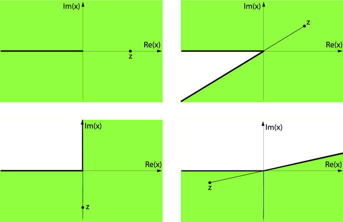

  

  The argument of the variable x is restricted to the sector $\arg x\in (\arg z-\pi ,\arg z+\pi )\bigcap (-\pi ,\pi ]$. The green region in all the pictures shows the different shapes of the $x-$section of the region $\Lambda _1$ for different arguments of z

  The remainder term is bounded in the form

  $$\begin{aligned} |R_n(\beta ',\beta ,\alpha ;x,y)|\le & {} \frac{e^{\pi \vert \Im \beta \vert }}{|\sin \theta |^{\Re \beta }} \frac{|\alpha |\,\,\Gamma (n+\Re \beta ') \vert x\vert ^n }{\vert \Gamma (\beta ')\vert \, n! \ (n+\Re \alpha )} \\&{}_3F_2\left( \left. \begin{array}{c} 1, n+\Re \beta ', n+\Re \alpha \\ \\ n+1 , n+\Re \alpha +1\end{array} \right| \left| x\right| \right) . \end{aligned}$$

Either, the right hand side of (37) or of (38) is a uniform convergent expansion of $F_1(\alpha ;\beta ,\beta ';\alpha +1;x,y)$ with an exponential order of convergence.

Proof

Comparing (36) to (10) we have that

$$\begin{aligned} F_1(\alpha ;\beta ,\beta ';\alpha +1;x,y)=\alpha \, F(\beta ',\beta ,\alpha -1;-x,-y). \end{aligned}$$

Then, the results follow from Theorems 3.1 and 3.2. $\square$

Note 4.1

Uniform expansions of the first symmetric standard elliptic integral $R_F(x,y,z)$ in terms of elementary functions are given in [5], and we refer the reader to this reference for details. Alternatively, those expansions can be derived from Theorems 3.1 and 3.2 by using the relation

$$\begin{aligned} R_F(x,y,z)=\dfrac{1}{2z^{1/2}}F\left( \frac{1}{2},\frac{1}{2},-\frac{1}{2};\frac{x-z}{z},\frac{y-z}{z}\right) . \end{aligned}$$

The function $R_{G}(x,y,z)$, [7, Sec 19.21, eq 19.21.11], may be written in the form

$$\begin{aligned} R_{G}(x,y,z)=\frac{1}{6}\sum x(y+z)R_D(y,z,x), \end{aligned}$$

where the summation extends over the three cyclic permutations of x, y, z. Therefore, uniform representations of the function $R_{G}(x,y,z)$ in terms of elementary functions can be directly derived from Corollaries 4.1 and 4.2.

Table 1 Relative error (with $G_2(x,y)=F_n(1/2,3/2,1/2,x,y)$ evaluated by using (30)) and relative error bound (31); for $x=1.8 e^{i\,\pi /5}$ and several values of $y =\vert y \vert \,e^{i\arg y }$ and order n of the approximation. We have taken the value of w(x) given by the second line of (12) and $\theta =\pi /2$ if $\Re y>0$ or $\theta =\text {arg }(y)$ otherwise

Table 2 Relative error (with $G_2(x,y)=F_n(1/2,3/2,1/2,x,y)$ evaluated by using (32)) and relative error bound (25) for $x=0.6 e^{i\,\pi /5}$ and several values of $y =\vert y \vert \,e^{i\arg y }$ and order n of the approximation. We have taken $w(x)=0$ and $\theta =\pi /2$ if $\Re y>0$ or $\theta =\text {arg }(y)$ otherwise

5 Final Remarks and Numerical Experiments

5.1 A Larger Domain of Applicability of Corollaries 4.1 and 4.2

An analytic representation of the first symmetric elliptic integral $R_F(x,y,z)$ is given in [5]. That expansion is first derived for $z>0$, and later extended to complex values of z in [5, Sec. 4] by using analytic continuation arguments. Identical arguments may be used here to enlarge the range of applicability of Corollaries 4.1 and 4.2 and deduce that the expansions derived for $G_1(x,y)$ in Corollary 4.1 hold, not only for $z>0$ and $x,y\in {\mathbb {C}}{\setminus }(-\infty , 0]$, but in the bigger domain:

$$\begin{aligned} \Lambda _1:=\lbrace (x,y,z)\in ({\mathbb {C}}{\setminus }(-\infty ,0])^3;\, \vert \arg x-\arg z\vert<\pi ,\,\,\vert \arg y-\arg z\vert <\pi \rbrace . \end{aligned}$$

Figure 2 illustrates the shape of the $x-$domain $\Lambda _1$ for fixed z (the $y-$domain for fixed z is analogous).

Fig. 3

Graphics of $G_1(x,y)=F(1/2,1/2,1/2;x,y)$ (black, dashed) and the approximations given by Corollary 4.1 with $n=1$ (blue), $n=2$ (brown) and $n=3$ (green) for different values of the fixed variable x and different intervals of the uniform variable y, with w(x) taken according to Lemma 2.2. We have taken $x=0.9$ and $y \in (-1,20)$ (top, left); $x=0.1$ and $y \in (-1,20)$ (top right); and $x=6.8 e^{\pi i /4}$ and $y \in (-5 e^{i\pi /3}, 5 e^{i\pi /3})$ (bottom). The bottom left picture corresponds to the real part of the functions, whereas the bottom right picture represents the imaginary part. The graphics are similar for others values of x and y. The graphics show the uniformly convergent character of the expansions in the variable y

Similarly, the expansions derived for $G_2(y,z)$ in Corollary 4.2 hold, not only for $x>0$ and $y,z\in {\mathbb {C}}{\setminus }(-\infty , 0]$, but in the bigger domain:

$$\begin{aligned} \Lambda _2:=\lbrace (x,y,z)\in ({\mathbb {C}}{\setminus }(-\infty ,0])^3;\, \vert \arg y-\arg x\vert<\pi ,\,\,\vert \arg z^3-\arg x^3\vert <\pi \rbrace . \end{aligned}$$

5.2 Numerical Experiments

Finally, in Tables 1 and 2 and Fig. 3, we give some numerical experiments that illustrate the accuracy and uniform character of the expansions derived in Theorems 3.1 and 3.2 (and therefore in Corollaries 4.1–4.3). In the numerical Tables 1 and 2 of this section we have computed the Relative Error ($E_{Rel}^n$) and compared to the relative error bound ($B_{Rel}^n$). They are defined in the form:

$$\begin{aligned} E_{Rel}^n:=\dfrac{|F_n(a,b,c;x,y)-F(a,b,c;x,y)|}{|F(a,b,c;x,y)|}, \qquad \qquad B_{Rel}^n:=\dfrac{|R_n(a,b,c;x,y)|}{|F(a,b,c;x,y)|}, \end{aligned}$$

where $F_n(a,b,c;x,y)$ represents the sum in the right hand side of (14) or (21), and $|R_n(a,b,c;x,y)|$ the corresponding error bound (16) or (22).

All the computations of this section have been carried out by using the symbolic manipulation program Wolfram Mathematica 12.2. In particular, the “exact” value of F(a, b, c; x, y) has been computed by means of numerical integration with the command “NIntegrate”.

References

Askey, R.A., Olde, A.B.: Generalized Hypergeometric Functions and Meijer G-Function, In: NIST Handbook of Mathematical Functions, Cambridge University Press, Cambridge, (2010), pp. 403–418 (Chapter 16)
Askey, R.A., Roy, R.: Gamma Fucntion, In: NIST Handbook of Mathematical Functions, Cambridge University Press, Cambridge, 136-147 (2010) (Chapter 5)
Bujanda, B., López, J.L., Pagola, P.: Convergent expansions of the incomplete gamma functions in terms of elementary functions. Anal. Appl. 16(3), 435–448 (2018)
Bujanda, B., López, J.L., Pagola, P.: Convergent expansions of the confluent hypergeometric functions in terms of elementary functions. Math. Comp. 88(318), 1773–1789 (2019)
Bujanda, B., López, J.L., Pagola, P., Palacios, P.: Uniform approximations of the first symmetric elliptic integral in terms of elementary functions. Rev. R. Acad. Cienc. Exactas Fís. Nat. Ser. A Mat. RACSAM 116(1), 1–17 (2022)
Byrd, P.F., Friedman, M.D.: Handbook of elliptic integrals for engineers and scientists. Springer, New York (1971)
Carlson, B.C.: Elliptic Integrals, In: NIST Digital Library of Mathematical Functions. https://dlmf.nist.gov/, Release 1.1.5 of 2022-03-15
Carlson, B.C.: A table of elliptic integrals of the second kind. Math. Comp. 49, 595–606 (1987)
Carlson, B.C.: A table of elliptic integrals of the third kind. Math. Comp. 51, 267–280 (1988)
Carlson, B.C.: A table of elliptic integrals: cubic cases. Math. Comp. 53, 327–333 (1989)
Carlson, B.C.: A table of elliptic integrals: one quadratic factor. Math. Comp. 56, 267–280 (1991)
Carlson, B.C.: A table of elliptic integrals: two quadratic factors. Math. Comp. 59, 165–180 (1992)
Carlson, B.C., Gustafson, J.L.: Asymptotic expansion of the first elliptic integral. SIAM J. Math. Anal. 16, 1072–1092 (1985)
Carlson, B.C., Gustafson, J.L.: Asymptotic approximations for symmetric elliptic integrals. SIAM J. Math. Anal. 25(2), 288–303 (1994)
Ferreira, C., López, J.L., Pérez Sinusía, E.: Uniform convergent expansions of the Gauss hypergeometric function in terms of elementary functions. Int. Transf. Spec. Func. 29(12), 942–954 (2018)
Ferreira, C., López, J.L., Pérez Sinusía, E.: Uniform representations of the incomplete beta function in terms of elementary functions. Elect. Trans. Num. Anal. 48, 450–461 (2018)
Fukushima, T.: Series expansions of symmetric elliptic integrals. Math. Comp. 81(278), 957–990 (2012)
Ghandehari, M., Logothetti, D.: How elliptic integrals K and E arise from circles and points in the Minkowski plane. J. Geom. 50, 63–72 (1994)
Gustafson, J.L.: Asymptotic formulas for elliptic integrals, Ph. D. Thesis, Iowa State Univ., Ames, IA, (1982)
Lawden, D.F.: Elliptic functions and applications. Applied Mathematical Sciences, vol. 80. Springer, New York (1989)
López, J.L.: Asymptotic expansions of symmetric standard elliptic integrals. SIAM J. Math. Anal. 31(4), 754–775 (2000)
López, J.L.: Uniform asymptotic expansions of symmetric elliptic integrals. Constr. Approx. 17, 535–559 (2001)
López, J.L.: Asymptotic expansions of Mellin convolution integrals. SIAM Rev. 50(2), 275–293 (2008)
López, J.L.: Convergent expansions of the Bessel functions in terms of elementary functions. Adv. Comput. Math. 44(1), 277–294 (2018)
López, J.L., Pagola, P.J., Palacios, P.: Uniform convergent expansions of integral transforms. Math. Comput. 90, 1357–1380 (2021)
Olde, A.B.: Hypergeometric Function, In: NIST Handbook of Mathematical Functions, Cambridge University Press, Cambridge, (2010), pp. 383–402 (Chapter 15)
Pólya, G., Szegö, G.: Inequalities for the capacity of a condenser. Amer. J. Math. 67(1), 1–32 (1945)
Razpet, M.: An application of elliptic integrals. J. Math. Anal. Appl. 168, 425–429 (1992)
Temme, N.M.: Special functions: An introduction to the classical functions of mathematical physics. Wiley, New York (1996)
Temme, N.M.: Large parameter cases of the Gauss hypergeometric function. J. Comput. Math. 153, 441–462 (2003)
Temme, N.M.: Asymptotic Methods for Integrals. World Sci, New Jersey (2015)
Urbina, A.M., et al.: Elliptic integrals and limit cycles. Bull. Austral. Math. Soc. 48, 195–200 (1993)
Van de Vel, H.: On the series expansion method for computing incomplete elliptic integrals of the first and second kinds. Math. Comput. 23(105), 61–69 (1969)
Weiglhofer, W.S.: Electromagnetic depolarization dyadics and elliptic integrals. J. Phys. A. 31, 7191–7196 (1998)
Wong, R.: Asymptotic approximations of integrals. Academic Press, New York (1989)
Acknowledgements
The anonymous referees are acknowledged for their careful examination of the manuscript and their improving suggestions.
Funding
Open Access funding provided by Universidad Pública de Navarra. This work was supported by the research grant RTI2018-095499-B-C31 Io Train and Universidad Pública de Navarra.
Author information
Authors and Affiliations
Contributions
All authors contributed to the study, conception and design. All authors read and approved the final manuscript.
Corresponding author
Ethics declarations
Competing Interests
The authors have no relevant financial or non-financial interests to disclose.
Additional information
Publisher's Note
Springer Nature remains neutral with regard to jurisdictional claims in published maps and institutional affiliations.
Rights and permissions
Open Access This article is licensed under a Creative Commons Attribution 4.0 International License, which permits use, sharing, adaptation, distribution and reproduction in any medium or format, as long as you give appropriate credit to the original author(s) and the source, provide a link to the Creative Commons licence, and indicate if changes were made. The images or other third party material in this article are included in the article’s Creative Commons licence, unless indicated otherwise in a credit line to the material. If material is not included in the article’s Creative Commons licence and your intended use is not permitted by statutory regulation or exceeds the permitted use, you will need to obtain permission directly from the copyright holder. To view a copy of this licence, visit http://creativecommons.org/licenses/by/4.0/.
About this article
Cite this article
Bujanda, B., López, J.L., Pagola, P.J. et al. An Analytic Representation of the Second Symmetric Standard Elliptic Integral in Terms of Elementary Functions. Results Math 77, 171 (2022). https://doi.org/10.1007/s00025-022-01707-3
Received:
Accepted:
Published:
DOI: https://doi.org/10.1007/s00025-022-01707-3
Keywords
- Symmetric standard elliptic integrals
- appell function
- convergent expansions
- uniform expansions