
Abstract
Magnets are at the core of both circular and linear accelerators. The main function of a magnet is to guide the charged particle beam by virtue of the Lorentz force, given by the following expression:where q is the electrical charge of the particle, v its velocity, and B the magnetic field induction. The trajectory of a particle in the field depends hence on the particle velocity and on the space distribution of the field. The simplest case is that of a uniform magnetic field with a single component and velocity v normal to it, in which case the particle trajectory is a circle. A uniform field has thus a pure bending effect on a charged particle, and the magnet that generates it is generally referred to as a dipole.
You have full access to this open access chapter, Download chapter PDF
8.1 Magnets, Normal and Superconducting
8.1.1 Introduction
Magnets are at the core of both circular and linear accelerators. The main function of a magnet is to guide the charged particle beam by virtue of the Lorentz force, given by the following expression:
where q is the electrical charge of the particle, v its velocity, and B the magnetic field induction. The trajectory of a particle in the field depends hence on the particle velocity and on the space distribution of the field. The simplest case is that of a uniform magnetic field with a single component and velocity v normal to it, in which case the particle trajectory is a circle. A uniform field has thus a pure bending effect on a charged particle, and the magnet that generates it is generally referred to as a dipole.
By equating the Lorentz force to the centripetal force, we obtain the bending radius ρ of the motion of a particle of charge q under the action of a magnetic field B perpendicular to the motion:
By expressing the momentum p in practical units [GeV/c], we can write:
where Z is the charge number of the particle, with q = Ze.
The product Bρ is known as magnetic rigidity and provides the link between dipole strength and length based on the momentum of a charged particle in a circular accelerator. Note how the formula shows clearly the trade-off between the bending magnetic field B and the size of the machine (related to ρ).
Besides bending magnets, a number of other field shapes are required to focus and control the beam. Most important are magnets that generate a pure gradient field, i.e. a field that is zero on the axis of the magnet and grows linearly with distance. This type of magnet is referred to as a quadrupole and is used to focus the particles on the central trajectory of the accelerator. The strength of a quadrupoles is customarily quoted in terms of the field gradient G, in units of [T/m]. A normalised quadrupole strength for a quadrupole of length l is defined as the ratio of the integrated quadrupole gradient to the beam rigidity, or: K = Gl/(Bρ). The angular deflection α (in radians) of a particle passing at a distance x from the centre of a quadrupole can be computed using the normalised quadrupole strength as:
which shows that a particle on the quadrupole axis (x = 0) has a straight trajectory, while a particle off-axis receives a kick proportional to its distance from the centre, i.e. the expected focussing effect. Higher order gradient fields, such as sextupoles, or octupoles, behave similarly and provide further non-linear means to control, correct and stabilize the dynamics of the motion of the particles, as described elsewhere in this handbook.
The accelerator magnets considered here have typically slender, long apertures (the space available for the beam), where the magnetic field has components only in the plane of the magnet cross section. In this plane, 2-D configuration, the most compact representation of the magnetic field shape in the magnet aperture is provided by the complex formalism [1] and its multipole expansion. Defining the complex variable z = x + iy, where the plane (x,y) is that of the magnet cross section, the function B y + iB x of the two non-zero components of the magnetic field is expanded in series:
The coefficients B n and A n of the series expansion are the multipoles of the field, and determine the shape of the field lines. As an example, a magnet in which only the term B 1 is non-zero, corresponds to a magnetic field:
i.e. a perfect dipole field (constant in amplitude and direction) oriented in y direction. If the y direction is taken perpendicular to the plane of the accelerator (e.g. vertical), this is usually called a normal dipole, which provides bending in the plane of the accelerator (e.g. horizontal). A magnet in which only A 1 is non-zero results in a perfect skew dipole field:
which is in the plane of the accelerator (e.g. horizontal) and provides bending perpendicular to it (e.g. vertical). Multipoles B 2 and A 2 correspond to magnets generating a pure normal and skew quadrupole field. Higher order gradients (sextupole, octupole, etc.) are obtained by simple analogy in the continuation of the series.
The explicit expressions of the field components corresponding to the first four multipoles, and a sketch of the corresponding field lines are reported in Table 8.1. It is useful to remark that the coefficients B n and A n appearing in Table 8.1 have units of [T/mn − 1] and are hence the generalized normal and skew gradient of order n. Specifically, B 2 corresponds to the normal quadrupole gradient G discussed earlier. To complete this short review of field configuration, we use the complex expansion to evaluate the module of the field B in the case of a pure normal multipole (chosen for convenience, the case of a pure skew multipole field yields identical results). Simple algebra, writing that z = Reiθ where R is the module and θ is the argument of z, gives the following result:
which shows that the field strength in a pure multipole field of order n is proportional to the generalized gradient and grows with the power n−1 of the distance from the magnet centre. This extends the case of the dipole (n = 1, constant field), and quadrupole (n = 2, linear field), to higher order multipoles such as the sextupole (n = 3, quadratic field profile), octupole (n = 4, cubic field profile), and so on.
Besides its compact form, the complex notation is useful because there is a direct relation between multipoles (order and strength) and beam properties. This is why accelerator magnets are often characterised using their harmonic content in terms of the B n and A n coefficients of the field expansion. Indeed, the pure multipolar fields discussed so far can only be approximated to a suitable degree in real magnets. The field generated by a magnet contains then all multipoles, normal and skew, i.e. a dense harmonic spectrum. Symmetries cause cancellation effects, resulting in low (ideally zero) non-allowed multipoles when compared to the multipoles allowed by the magnet symmetry. Selected multipoles can be further reduced by using design features such as optimization of the coil and iron geometry, or corrections such as passive and active magnetic shims.
We define the field quality of an accelerator magnet as the relative difference between the field produced and the ideal field distribution, usually a pure multipole, in the region of interest for the beam, which is generally referred to as the good field region. Depending on the shape of the good field region, it may be convenient to quote field quality as an overall homogeneity (i.e. ΔB/B, typically done for magnets with a rectangular or elliptic aperture), or providing the spectrum of multipoles other than the one corresponding to the main magnet function (ratio of A n and B n to the main field strength, typically done for magnets with round bore). Whichever the form, the field quality of accelerator magnets is generally requested to be in the range of few 10−4. To maintain practical orders of magnitude, field errors are then quoted in relative units of 1 × 10⁻⁴ of the main field, or simply units.
Gradient magnets (i.e. quadrupole and higher order) are also characterised by a magnetic axis, which is usually taken as the locus of the points in the magnet aperture where the field is zero. Magnets are aligned with respect to their axis (or an average of the locus when it deviates from a straight line) to the specified beam trajectory to avoid unwanted feed-down effects. Typical alignment tolerances in circular machines range from few tens of μm in synchrotron light sources to fractions of mm in large colliders (e.g. the LHC). Linear colliders are more demanding, with typical tolerances at the sub-μm level.
Dipoles and quadrupoles are the main elements of the linear optics in modern synchrotrons. Depending on the beam specifications, any residual field and alignment imperfections, as well as drift in magnet properties, may require active correction to ensure stable and efficient operation. This is done using corrector magnets that are powered using information established from previous knowledge on the main magnets, or parameters measured on the beam, or both. Corrector magnets are often designed to generate a single multipole, so to act on the beam as an orthogonal knob, thus making the correction easier to execute.
8.1.2 Normal Conducting Magnets
“Normal conducting”, and alternatively “resistive”, “warm” or “conventional” magnets, are electro-magnets in which the magnetic field is generated by conductors like copper or aluminium, which oppose an electrical resistance to the flow of current. The magnetic field induction provided in the physical aperture of these magnets rarely exceeds 1.7 to 2.0 T, such that the working point of the ferromagnetic yoke remains below saturation. In these conditions, the yoke provides a closure of the magnetic path with small use of magneto-motive force, and its pole profile determines the magnetic field quality.
The integral form of the static part of the last Maxwell equation, the Ampere’s law, provides a simple analytical expression for the relationship between magnetic field and magneto-motive force in most of magnet configurations used in particle accelerators.
As an example, we illustrate in Fig. 8.1 a non-saturated C-type dipole magnet, made of two coils of N/2 turns each, connected in series and supplied by a current I.

C-dipole magnetic circuit, of physical vertical aperture l air, supplied with a total magnetomotive force NI
If μ r ≫ l iron/l air we can neglect the magneto-motive force “used” in the iron and obtain:
If part of the iron is saturated, its permeability will be lower and part of the ampere-turns NI will be used to magnetize the iron as discussed later.
In case the magnetic field exceeds a value of typically about 1.5 T along the path corresponding to l iron the magneto-motive force used in the iron may become no longer negligible with respect to that used in the air. As the iron yoke gathers also the stray field, the field induction in the iron poles is always higher than the one between poles. To reduce the iron portion working at fields above 1.5 T, the iron pole can be tapered. This allows designing iron-dominated magnets capable of producing magnetic fields intensities in their physical aperture rather close to the saturation limit of the iron, i.e. up to about 1.7–2.0 T. A quantitative example of the effect of saturated iron in dipole magnet is given in Fig. 8.2.

C-dipole magnetic circuit of physical vertical aperture l air = 10 mm, supplied with N tot I = 12,000 A
8.1.2.1 Magnetic Design
Transfer function (the ratio of the magnetic field intensity in the magnet aperture to the supply current) and inductance can be computed starting from the Ampere’s law and considering the relationship between magnet inductance (L), current (I) and energy (E) as E = ½·LI 2.
In practical cases the theoretical transfer function of an ideal magnetic circuit is reduced by an “efficiency” η, typically of the order of η = 0.95…0.98, which depends on the length, stacking factor and working conditions of the magnetic yoke. The formulas in Table 8.2 provide an analytical formulation of the inductance values for different magnet configurations.
The inductance depends on how the pole geometry is trimmed (shims, tapered poles, chamfers) and on saturation. For quadrupole and sextupole magnets different tapering of the poles can strongly modify the inductance. For such magnets these simplified formulas can cover only standard designs.
The field homogeneity typically required by an accelerator magnet within its good field region is of the order of few parts in 10−4. Transfer line and corrector magnets may be specified with lower homogeneity.
Field quality in a given volume is determined by several factors:
-
the size of the magnet aperture with respect to the good field region
-
the shape of the iron poles
-
manufacture and assembly tolerances
-
the position of active conductors (coils), in particular in window-frame magnets
-
the ferromagnetic properties at the working conditions of the steel used for the yoke
-
dynamic effects
Optimizing field quality is achieved considering all above aspects. In particular magnets operating below 2 T, as the ones treated in this chapter, are also described as iron dominated magnets because the shape of the magnetic field induction is dominated by the shape of the ferromagnetic poles. At the interface between the magnet aperture and the poles, i.e. between steel and air, the component of the magnetic field induction B ⊥ perpendicular to the interface surface is the same on both media. The tangential component of the magnetic field H t also remains the same in case no surface currents are present: this corresponds to a change of the tangential components Bt of the field induction by the ratio of the magnetic permeability between the two media. As a result, in case of infinite permeability the direction of the magnetic field induction in the air at the exit of a magnet pole is always perpendicular to the pole surface.
An example of trimming field quality with pole shims in a dipole magnet is shown in Fig. 8.3.

C-dipole with pole shims. The shims extend the good field region
8.1.2.2 Coils
The coils generate the magneto-motive force necessary to produce the required magnetic field induction in the magnet physical aperture. Coils produce losses due to their electrical resistance.
The power dissipated in a conductor of electrical resistivity ρ, volume V, effective current density J rms, is:
where S is the conductor section, l its length, I rms = SJ rms the effective current, R the electrical resistance. In case the current is not uniformly distributed in the conductor section, in particular for fast transients where the penetration depth is smaller than the conductor size, an effective section has to be considered.
We recall the resistivity of copper and aluminium as a function of the temperature T:
The effective current density J rms determines coil size, power consumption and cooling: the designer shall consider the right balance between requirements, technological limits, investment and operation cost.
Typical values of J rms are around 5 A/mm2 for water cooled magnets, and around 1 A/mm2 for air cooled magnets. Air cooled coils with favourable configurations (large heat exchange surface with respect to their section) can be operated at higher current densities.
Introducing l av as the average coil turn length, it is easy to show that the power dissipated in a magnet is:
In case of water-cooled magnets, heat is removed by water circulating in the coil (hollow) conductors.
The choice of cooling parameters and number of circuits is based on a few main principles: set the water flow corresponding to the allowed temperature drop for a given power to be removed, having a moderate turbulent flow to provide an efficient cooling, keeping the water velocity within reasonable limits to avoid erosion-corrosion and impingement of the cooling pipes and of the junctions, keeping the pressure drop across the circuit within reasonable limits (typically within 10–15 bars). Properties of water cooling circuits are provided in Table 8.3
Finally, we remark that coils are submitted to forces: their own weight and the electromagnetic forces produced by the interaction between magnetic field and current.
The interaction between a moving charge and the magnetic field is described by the so called Lorentz force, which in the macroscopic form for a wire carrying a current I is referred as Laplace force:
where the length l is oriented towards the direction of the current flow. For example 1.5 m of straight coil immerged in an average magnetic field component perpendicular to the coil of 0.5 T, carrying a total current of 60,000 ampere-turns, is subjected to a force of F = 60,000 ∙ 1.5 ∙ 0.5 = 45 kN.
8.1.2.3 Yoke
The magnet yoke has the function of directing and shaping the magnetic field generated by the coils. While magnets operated in persistent mode can be built either with solid or with laminated steel, the yokes of cycled magnets are composed of laminations electrically insulated from each other to reduce the eddy currents generated by the change of magnetic field with time. This electrical insulation can be inorganic (oxidation, phosphating, Carlite) or organic (epoxy). Epoxy coating in a B-stage form can be used to glue laminations together, a technique widely used for small to medium magnets, possibly reinforced by welded bars on the yoke periphery.
The magnetic properties of steel depend on the chemical composition and on the temperature/mechanical history of the material. Important parameters for accelerator magnets are the coercive field H c and the saturation induction. The coercive field has an impact on the reproducibility of the magnetic field at low currents. A typical requirement for the steel used in accelerator magnets is H c < 80 A/m. Tighter constraints (H c < 20 A/m) apply when the operation covers a large field factor starting from low field inductions (few hundred gauss). The saturation induction is highest with low carbon steel (carbon content in the final state <0.006%). It is common to specify points along the normal magnetization curve, with the condition that the magnetic induction B shall exceed specification values at given field levels H.
To increase its electrical resistivity and at the same time narrow the hysteresis cycle, laminated steel used in cycled magnets usually contains 2…3% of silicon.
With 3% of Si the electrical resistivity increases from ρ = 2 ∙ 10−7 Ωm to ρ = 5 ∙ 10−7 Ωm.
The work performed during the hysteresis cycle and the eddy currents produce losses in cycled magnets. An estimate of hysteresis losses can be obtained by the Steinmetz law:
where f is the frequency and η = 0.01…0.1, about 0.02 for silicon steel, and of eddy current losses, for silicon steel, by:
where d lam is the lamination thickness in mm.
8.1.2.4 Costs
We can distinguish
-
fixed costs: design, coil tooling (winding, molding), yoke tooling (punching, stacking), quality assurance (including tools for specific measurements/checks, as magnetic measurements if requested);
-
unitary costs: main materials (conductor, insulation, steel), manufacture of parts (coil, laminations, yoke), final assembly, ancillaries (connectors, interlocks, hoses), tests (mechanical, electrical, magnetic);
-
other systems: cooling, power converters, controls and interlocks, electrical distribution. These parameters have to be taken into account at the magnet design phase: for example for cycled magnets a low inductance can minimize the voltage levels, however the corresponding higher current would require larger supply cables from the power converters to the magnets.
-
running costs: electric power, maintenance over the life of the project.
A compromise between capital and operational cost is typically found with magnets operating with:
-
current densities of about 5 A/mm2: higher current densities correspond to smaller coils and consequently smaller and cheaper yokes, lower current densities correspond to lower power consumption (less electricity, smaller cooling plant) but to larger magnets;
-
field induction levels in the region between 1.2 T and 1.7 T: a given required integrated strength can be provided by short magnet with high field induction, long magnets with low field induction or a compromise between the two. Since, below saturation, the pole width size depends essentially on the good field region size and not on the field induction level, the highest possible field and the corresponding lowest magnetic length represent in most cases a cost-optimized yoke design.
8.1.2.5 Undulators, Wigglers, Permanent Magnets
Wigglers and undulators produce a periodic field variation along the beam trajectory causing relativistic charged particles to wiggle emitting electromagnetic radiation with special properties, in particular with a small angle α = 1/γ where γ is the relativistic factor.
To a first approximation, these magnets produce a series of dipole fields with alternated directions, of period λ. This is typically obtained with conventional electromagnets when the period is relatively large allowing sufficient space for the coils, and with permanent magnets for shorter periods. Superconducting windings, in general cryo-cooled, are used in case the required field exceeds 2 T and/or for small periods where a high current density is needed.
The difference between wigglers and undulators is in the nature of the radiation produced by the particle. When the amplitude of the beam excursion expressed in meters is small with respect to the angle of the synchrotron radiation emission expressed in radians, the device is called undulator: the emitted radiation is concentrated in a small opening angle and the radiation produced by the different periods interferes coherently producing sharp peaks at harmonics of a fundamental wavelength. Wigglers on the contrary produce particle displacements of larger amplitude: the emitted radiation is similar to the continuous spectrum generated by bending magnets, with in addition the effect coming from the incoherent superposition of radiation from individual poles.
It is useful to introduce the deflection parameter K = δ 0/α as the ratio between the maximum trajectory deflection δ 0 (in meters) and the emission angle α (in radians). For electrons:
In case K < 1 the device is an undulator, in case K >> 1 the device is a wiggler.
As anticipated, these magnets are often built with the use of permanent magnets.
Two types of high performance permanent magnet materials, both composed of rare earth elements, are available: Neodymium-Iron-Boron (NdFeB) and Samarium-Cobalt (in the form SmCo5 or Sm2Co17, also referred as SmCo 1:5 and SmCo 2:17).
NdFeB materials show the highest remanent induction, up to B r~1.4T, and the highest energy product up to BH max~50 MGOe, they are ductile, but they require coating to avoid corrosion and have a relatively low stability versus temperature. Their relative change of remanent field induction with temperature (temperature coefficient) is ΔB r/B r~ − 0.11% per °C: field induction decreases when temperature increases.
SmCo magnets show a lower remanent induction, up to B r~1.1 T, are brittle, but they are corrosion and radiation resistant. Furthermore, their temperature coefficient is about −0.03%, lower than that of NdFeB.
The use of permanent magnets in particle accelerators is not limited to wigglers and undulators. For example, the 3.3 km long recycler ring at FNAL, commissioned in May 1999, stands as a pioneer, as it is solely composed of permanent magnets dipoles and quadrupoles [2]. More recently, permanent magnets are used in compact quadrupoles for LINAC4 at CERN [3], in the main bending magnets of the ESRF-EBS light source [4], and even as spectrometers as for example in the nTOF experiment at CERN [5].
8.1.2.6 Solenoids
Solenoids are made by electrical conductors wound in the form of a helix. The magnetic field induction inside an ideal solenoid is parallel to the longitudinal axis and its intensity is B = μ 0 NI/l where NI is the total number of ampere-turns and l the solenoid length. By introducing the coil thickness t, the formula can be written as B = μ 0 Jt, where J is the current density.
Solenoids can be built as ironless magnets or can have an external ferromagnetic yoke, used for shielding and to increase the magnetic field uniformity particularly at the solenoid extremities.
The design and construction of solenoids, thanks to their use in many electrical and electro-mechanical devices, is well assessed since more than a century. A comprehensive treatment of solenoid electromagnets was compiled by C. Underhill already in 1910. The treatment issued by Montgomery in 1969 is still a reference [6] nowadays, in spite of new materials now available in particular for wire dielectric insulation and for the containment of stresses.
In solenoids the electromagnetic forces produced by the interaction between the magnetic field and the currents in the coils can reach extremely high values capable of breaking the wires or even, especially for pulsed magnets, leading to an explosion of the device. Their design should consider conductor characteristics and reinforcements, winding tension during manufacture and the containment structure.
8.1.3 Superconducting Magnets
Superconducting magnet technology has been instrumental to the realization of the largest particle accelerators on Earth. Table 8.4 reports the main characteristics of the four large scale hadron accelerators built and operated since the beginning of superconducting magnet technology for accelerators. In parallel, superconductivity has fostered the construction of high field and large volume detector magnets that have become commonplace in high energy physics. The first such detector magnet was installed at Argonne National Laboratory, and operated in the mid 1960s as an instrument in the Zero Gradient Synchrotron (ZGS) [11]. Atlas [12] and CMS [13] at the LHC are the latest and most impressive example of superconducting detector magnets.

Cross section (to scale) of the dipoles of the four major superconducting hadron accelerators built to date
The prime difference between superconducting and normal conducting magnets is in the way the magnetic field induction is generated. While in normal conducting magnets the field is dominated by the magnetization of the iron yoke, in their superconducting “siblings” the field is generated by a suitable distribution of currents, properly arranged around the beam aperture. This is possible because a superconducting material can carry large currents with no loss, and ampere-turns become cheap, thus opening the way to magnetic fields much above saturation of ferromagnetic materials. Very schematically, superconducting magnets for large scale accelerators consist of a coil wound with highly compacted cables, tightly packed around the bore that delimits a vacuum chamber hosting the beam. The coil shape is optimized to maximize the bore field and achieve acceptable field quality, as described later. The large forces that are experienced by the coil (several tens to hundreds of tons/m) cannot be reacted on the winding alone, that has the characteristic shape of a slender racetrack. The force is hence transferred to a structure that guarantees mechanical stability and rigidity. The iron yoke that surrounds this assembly closes the magnetic circuit, yields to a marginal gain of magnetic field in the bore, and shields the surrounding from stray fields. Finally, the magnet is enclosed in a cryostat that provides the thermal barrier features necessary to cool the magnet to the operating temperature, which is in the cryogenic range (1.9 to 4.5 K for accelerators built to date). Various implementations of this basic concept can be seen in Fig. 8.4 that shows the cross sections of the superconducting dipoles of the four large superconducting hadron accelerators listed in Table 8.4.
Superconducting magnet technology relies heavily on the ability to produce technical superconducting materials in the form of high current cables. Beyond considerations on the magnetic field that are specific to the arrangements described above, the design of superconducting magnets must take into account issues related to the superconductor, such as stability, quench protection, magnetization and AC loss. The magnet powering requires warm-to-cold transitions capable to transport the large currents in the range of few to few tens of kA with minimal thermal loss. The construction of the magnet, and in particular the insulation, coil winding, assembly in the mechanical structure and yoke, and the placement in a cryostat necessary for thermal management, all have aspects specific to superconducting magnet technology. Finally, cooling by helium is a science by itself. In the following sections we will discuss some of the main principles, without entering into detail, and provide extensive references on the above matters. The bibliography in the references directs the reader to excellent books on superconducting magnet engineering and science, especially [14,15,16,17,18].
8.1.3.1 Superconducting Materials
A superconductor is such only if it operates below the critical surface, a combination of temperature T, magnetic field induction B and current density J that delimits the boundary between the superconducting and normal-conducting phases. This surface is best expressed using a function J C(B,T), the critical current density which is the main engineering characteristic of a superconductor. A good example is the critical current density for the highly optimised Nb-47%Ti alloy used for the production of the LHC magnets, shown in Fig. 8.5. When cooled to 4.2 K, this superconductor can carry a current density up to 3000 A/mm2 in a background field of 5 T. Indeed, this is the order of magnitude of current density that is of interest to make the design of a superconducting accelerator competitive. As we see from Fig. 8.5, higher fields or higher temperatures result in a reduction of the critical current density, while a decrease of any yields an increase in J C.

Critical current density of Nb-47%Ti representative of the LHC production. The superconductor carries 3000 A/mm2 at a temperature of 4.2 K and in a background field of 5 T (marked point). The LHC dipoles operate at 1.9 K, taking advantage of the increase of J C at lower temperature to reach a nominal field of 8.33 T
Table 8.5 reports a summary of the critical temperature T C and critical field B C for the technical superconducting materials that have found practical applications over the past 50 years, as well as materials that are expected to come into use in a few years. The materials are generally classified as low-temperature superconductors (LTS) and high-temperature superconductors (HTS). This classification was originally based on the temperature of the superconducting transition TC, but now it refers rather to the different mechanisms that explain the existence of a superconducting phase. According to this classification, the alloy of Niobium and Titanium (Nb-Ti), the inter-metallic compounds of Niobium and Tin or Aluminium (Nb3Sn, Nb3Al) and of Magnesium and Boron (MgB2) are LTS materials. On the other hand, the Perovskites formed by Bismuth, Strontium, Calcium and Copper oxide (conventionally referred to as BSCCO) and a Rare Earth (e.g. Yttrium), Barium and Copper oxide (referred to as REBCO) are HTS materials. The details of the material composition and production route influence the values of T C and B C. For this reason the values quoted in the table should be regarded as indicative, especially for developmental materials such as MgB2, BSCCO and REBCO.
Note for completeness that many other elements and compounds become superconducting when cooled to sufficiently low temperatures and, in some cases, when submitted to large pressure. The family of superconductors is hence still developing. The recent discovery of a new class of HTS, the iron based superconductors [25] (also named IBS, FeSC, or ferropnictides), bears the promise of understanding the theory of high-temperature superconductivity, as well as the potential development of a new class of technical materials for high field applications. At the time of writing, the search for the highest possible T C has reached the maximum verified value of 203 K in a hydrogen sulphide under a pressure of the order of 155 GPa[26].
Though exciting and promising, these recent developments are still far from being ripe for applications. In the following sections we will focus on the main characteristics of the technical superconductors of Table 8.5, which are at present the only ones available in sufficient quantity and quality for magnet applications.
8.1.3.1.1 Nb-Ti
The alloy of Nb-47%Ti [19] is undoubtedly the most successful practical superconductor, and has been used in all superconducting particle accelerators built to date. Nb-Ti is a ductile and tough material, easily available in long lengths (a few km piece length) in the form of multi-filamentary wires where the superconductor is dispersed in a copper matrix of high purity and low electrical resistivity. Nb-Ti at 4.2 K has a critical current density of about 1500 A/mm2 at 7.5 T. Cooling it to 1.9 K shifts this point up to 10.5 T. This field range represents the upper (quench) limit for the use of Nb-Ti in accelerator magnets. Standard industrial production yields filament size of a few μm (5 to 10), which is beneficial to reduce the field perturbations induced by persistent currents (see later). Smaller filaments (1 to 3 μm) have been produced to reduce magnetization and losses, but this R&D products are not industrial standards. Homogeneity of the production is at the level of few % for key parameters such as critical current, magnetization, wire composition and geometry, which demonstrates the maturity of the technology. Figure 8.6 shows multi-filamentary Nb-Ti strands used in the LHC.

One of the multi-filamentary Nb-Ti strands used in the LHC. The strand has a diameter of approximately 1 mm, and each Nb-Ti filament (shown in the detail micrograph) has a diameter of 7 μm. The matrix is pure copper
8.1.3.1.2 Nb3Sn
The inter-metallic compound Nb3Sn [20] is the second LTS material that founds its way from material research to large-scale applications. Nb3Sn is a brittle and fragile compound, which is why after an initial success in high field solenoids of the 1960’s, attaining record fields of 10 T, it was quickly replaced by the ductile Nb-Ti for more modest field values. All manufacturing routes involve assembly of the precursor elements Nb and Sn into large size billets that are extruded and/or drawn to the final diameter wire. The Nb3Sn is then formed by a chemical reaction induced by a heat treatment to temperatures in the range of 650 °C for durations of few tens to few hundreds hours. Various manufacturing routes have been established industrially, resulting in wires with different properties of critical current density and filament size. Most common fabrication methods are based on the so-called “bronze-route”, or “internal-tin”, which distinguish themselves by the way that the relatively mobile Sn is made available for reaction with Nb. The interest in Nb3Sn comes from the improved TC and BC with respect to Nb-Ti, resulting in record critical current density exceeding 1500 A/mm2 at 15 T and 4.2 K. This potential is commonly exploited in commercial solenoids built for NMR spectroscopy or other laboratory applications, but to date found no accelerator applications due to the technical difficulties associated with the heat treatment and the handling of a fragile magnet coil. In addition, high JC Nb3Sn has presently larger filament size than Nb-Ti, in the range of 50 to 100 μm. This material is nonetheless very relevant to extend the reach of present accelerators such as the LHC beyond the limit of Nb-Ti (e.g. the High-Luminosity upgrade of the LHC and the R&D on magnet technology for a Future Circular Collider), or to build compact accelerators that could be of interest for industrial and medical applications (e.g. high-field compact cyclotrons for proton therapy).
8.1.3.1.3 MgB2
The most recent of the technical superconductors [22], the inter-metallic compound MgB2 is a relatively inexpensive material obtained from readily available precursor elements. Superconducting MgB2 wire can be produced through the powder-in-tube (PIT) process. Variants of this process exist, depending on whether the MgB2 is formed at the end of the wire processing from Mg and B precursors (in-situ variant), or rather powders of pre-reacted MgB2 are sintered in the finished wire (ex-situ variant). In both cases, a heat treatment is required in the range of 600 °C to 1000 °C. As for Nb3Sn, the wires and tapes of MgB2 are fragile and require careful handling to limit deformation. In spite of a high critical field, which in thin films has reached values above 70 T, the bulk material becomes irreversible at much smaller applied fields. MgB2 is hence of interest in the range of low to medium field applications (presently up to a maximum 5 T range), but for operating temperatures up to 20 K, i.e. well above boiling helium conditions. The main technical realizations presently based on MgB2 are open MRI systems at modest magnetic field (0.5 T), and cables for power transmission planned for the High Luminosity upgrade of the LHC (the so called SC links) or electric energy distribution. This material is to date still in the developmental state, with specific interest in enlarging the field range for magnet applications. While the main motivation remains helium-free MRI magnets, MgB2 could be an option for accelerator magnets subjected to radiation loads that require high operating temperature and energy margin (see later).
8.1.3.1.4 Cuprate Superconductors
These are the two HTS materials that seem to bear the largest potential for future use in accelerator magnets, mainly because of the high critical field at low operating temperature that makes them the ideal candidates to break the 20 T barrier. Both BSCCO and REBCO are ceramic compounds obtained respectively by chemical synthesis of B, Sr, Ca, Cu and O, or Y, Ba, Cu and O. As for all other HTS materials, their production is a complex process that may involve assisted crystal growth, at high temperature, and under very well controlled chemical conditions. BSCCO and REBCO still have unresolved engineering issues, they are fragile, and have comparatively high material and production costs. One of the main limitations to critical current in HTS materials comes from the effect of grain boundaries. Mis-aligned grain boundaries are a barrier to the free flow of the super-currents. In principle, this means that HTS conductors would require solving the tantalizing task of growing single crystals of km length. Different ways have been found to deal with this limitation in BSCCO and REBCO. BSCCO is manufactured using a Powder in Tube (PIT) technique, filling Ag tubes with a precursor BSCCO oxide powder. Two different techniques are used to produce the 2212 and 2223 variants of the BSCCO compound. In the case of BSCCO-2212, the tubes are stacked and drawn to wires that can be wound, cable and finally reacted, much like Nb3Sn, albeit at higher temperature (900 °C) and under controlled oxygen atmosphere. BSCCO-2212 undergoes a melt process, critical to produce the connected grain structure required for high critical current. For BSCCO-2223 the common form is tape. An initial liquid-mediated reaction of the precursor is used to form the 2223 compound. In this case the required grain alignment cannot be obtained upon heat treatment, but can be induced by mechanical deformation. This is why reacted BSCCO-2223 is mechanically deformed to the final tape dimension, and undergoes a final sintering heat treatment. REBCO is also manufactured in the form of tape. A robust substrate such as stainless steel or hastelloy, is polished and prepared with a series of buffer layers that imprint a crystal texture to a thin layer of REBCO superconductor. This is the crucial step to induce aligned crystal growth of the superconducting phase. The superconductor growth can be achieved by various chemical or physical deposition techniques. The tape is then capped with a sealing Ag layer, finally adding Cu as a stabilizer. When cooled down to 4.2 K, REBCO and BSCCO attain exceptional current densities at high-field, surpassing the performance of LTS materials at fields of 10 to 15 T. In spite of the early phase of development, the HTS BSCCO-2223 already found a large-scale application in the current leads of the LHC, where the gain in operating efficiency and margin has offset the additional investment.
8.1.3.2 Superconducting Cables
Wires and tapes manufactured with the LTS and HTS materials listed above carry currents in the range of few hundreds of A, and are appropriate to wind small magnets, where the magnet inductance and stored energy are not an issue (see later discussion on protection). On the other hand, the large-scale dipole and quadrupole magnets of an accelerator are connected in km-long strings, and stored energy that can reach hundreds of MJ. To decrease their inductance and limit the operating voltage, it is mandatory to use cables made of several wires in parallel, able to carry much larger currents, typically in the range of 10 kA. An additional benefit of a cable is to provide parallel paths for the current in case of local wire defects. Such cables must insure good current distribution through transposition, combined with precisely controlled dimensions necessary to obtain coils of accurate geometry, as well as good winding characteristics. These properties are the characteristic of the flat cable invented at the Rutherford Laboratory in England [27]. A typical Rutherford cable, shown in Fig. 8.7, is composed of fully transposed twisted wires (Nb-Ti in Fig. 8.7). The transposition length, also referred to as twist pitch, is usually kept short, a few cm. To improve winding properties the cable is slightly keystoned, i.e. the cable width is not constant from side to side. The angle formed by the planes of the cable upper and lower faces is called the keystone angle, usually in the range of 1 to 2 degrees. A summary of cable characteristics for the major superconducting accelerator projects is reported in Table 8.6.

The Rutherford cable for the inner layer of the LHC dipoles, showing the Nb-Ti filaments in a few etched strands. The schematic in the inset shows the definition of the quantities reported in Table 8.6
The concept of Rutherford cables can be easily applied to LTS materials that come in the form of round wires and has been recently extended to round BSCCO-2212 HTS wires. The rectangular geometry of the cable provides high strand packing and a flexible cable for winding magnet coils of various geometries. The cabling process is invariably associated with large deformations at the edges of the cable, where the wires are plastically deformed. This is necessary to achieve mechanical stability of the cable, but can lead to a degradation of the critical current of the superconductor. Optimization of this delicate balance between limited wire deformation and desired cable compaction is done empirically, and the I C degradation in an optimized cable is in the range of a few %.
The electro-dynamic and mechanical requirements for a cable are essentially independent of the superconducting material, at least to first order, and apply both to LTS and HTS. Cabling of HTS materials, however, and in particular those only available in the form of tapes, is far by being standard practice. Several configurations are under development, from compact stacks and Roebel bars, to twisted assemblies of tapes, or wound tapes around cores. Indeed, the matter of HTS cabling is an R&D that will need to be resolved before these materials can become a viable superconductor for accelerator magnets.
8.1.3.3 Stability and Margins, Quench and Protection
We have already remarked that a superconductor is such only when it operates below its critical surface. Once in normal conducting state, e.g. because of a sudden temperature increase caused by internal mechanical energy release or a beam loss, the superconductor generates resistive power, causing a thermal runaway, i.e. an unstable behaviour. It is for this reason that the operating point of current density J op, field B op and temperature T op are chosen by design well inside the allowable envelope, i.e. with proper margins that ensure stability at the operating point. The typical metrics used for operating margins are:
-
Critical current margin i, expressed as the operating fraction of the critical current density i = J op/J C(B op,T op), where the critical current is evaluated at the operating field and temperature;
-
Margin along the loadline f, expressed as the ratio of operating to critical current f = J op/J C(t/J C,T op) where the critical current is evaluated at the intersection of the magnet loadline, i.e. the straight line with slope t = B/J and the critical surface;
-
Temperature margin ΔT, given by the difference in temperature from operating conditions T op to current sharing conditions T CS, evaluated at the operating field and current density ΔT = T CS(J op,B op) − T op. The current sharing temperature is defined as the temperature at which the operating current density equals the critical current, or J op = J C(B op,T CS).
The margins defined above are shown graphically in Fig. 8.8. Representative values for the design of the large-scale Nb-Ti accelerator dipoles listed earlier are i ≈ 0.5, f ≈ 0.8, and ΔT = 0.5…1.5 K.

Definition of the operating margins discussed in the text
An additional quantity that measures the stability of the operating point is the energy margin, i.e. the quantity of heat necessary to drive the superconductor normal. The energy margin depends on the time and space structure of the heat deposition. A lower bound of the energy margin is given by the enthalpy difference between operating and current sharing conditions ΔH = H(T CS) − H(T op). A robust magnet design is such that the energy margin is larger than the expected amplitude of perturbation over the whole spectrum of operating conditions and characteristic times, which is the basic idea behind all stabilization strategies adopted.
In spite of good design, an irreversible transition to the normal conducting state is always possible, resulting in a thermal runaway process that is referred to as a quench. Superconducting magnets in general, and more specifically the highly compact accelerator magnets, tend to have large stored magnetic energy density. Local dissipation of this energy has the potential to lead to material damage and cause loss of electrical insulation. For this reason all superconducting magnets must be protected against quench by detecting any irreversible resistive transition (quench detection electronics) and discharging the magnet. The peak temperature T hot reached during a quench can be estimated by equating the Joule heat produced during the discharge to the enthalpy of the conductor, or H(T hot) − H(T op) = ∫ρJ 2 dt, where ρ is the specific resistance of the superconductor composite in normal conducting state. We see from the above concept, borrowed from electrical blow-fuses design, that it is always advantageous to reduce the normal state resistance and the time of the discharge. The normal state resistance is decreased by backing the superconductor with a matrix of a material with good conductivity properties (e.g. copper, aluminium or silver). The discharge can be made faster by reducing the inductance of the magnet, which is the reason why large scale magnets are wound using cables with large operating current in the place of single wires. There are various possibilities to dump the magnetic energy, based on one or more of the following standard strategies:
-
Energy extraction, in which the magnetic energy is extracted from the magnet and dissipated in an external circuit (e.g. a dump resistor or diode);
-
Coupling to a secondary circuit, in which the magnet is coupled inductively to a secondary that absorbs and dissipates a part of the magnetic energy;
-
Subdivision, a partition of the magnet in sections, with each section shunted by an alternative current path (resistance or diode) in case of quench;
-
Active quench initiation, that relies most commonly on heater embedded in the winding pack, fired at the moment a quench is detected to spread the normal zone over the whole magnet mass and thus reduce the peak temperature. Alternative means to actively initiate quench have been revisited, based on over-current or fast field changes induced by capacitive discharge in the coil.
8.1.3.4 Magnetization, Coupling and AC Loss
An ideal superconductor (type-I) tends to exclude field variations from its bulk, i.e. a perfect diamagnetic behaviour. In practice, in the superconducting materials listed above (type-II) the magnetic field can penetrate the bulk, still resulting in partial diamagnetism. Macroscopically seen, a field change induces shielding currents, which, in a superconductor, do not decay. For this reason these currents are referred to as persistent. The magnetic moment per unit volume M associated with persistent currents is proportional to the current density J C of the shielding currents, and the characteristic size D of the superconductor, i.e. M ≈ J C D. This magnetic moment can attain large values, perturb the field generated by the magnet, and lead to instabilities in case the magnetic energy inside the superconductor is dissipated in a process referred to as flux-jump. For this reason, the superconductor in wires and tapes is subdivided in fine filaments that have characteristic dimension in the range of 10 to 100 μm. Persistent currents and the associated magnetization produce a significant field perturbation in accelerator magnets, and must be subject to optimization and tight control.
Similar to the bulk behaviour described above, field variations also induce shielding currents between the superconducting filaments. These currents couple the filaments electromagnetically by finding a return path crossing the wire matrix. The amount of filament coupling depends on the resistivity of the matrix, which has to be low for good protection, and the geometry of the current loop. In the extreme case of wires and tapes with untwisted filaments, coupling currents could travel along long lengths (e.g. the km length in a magnet) and find a low cross-resistance. The net effect would be that the multi-filamentary matrix would respond to field changes as a single bulk filament, losing the advantage of fine subdivision. Decoupling of the filaments is achieved by shortening the current loop, twisting the wire with typical pitch in the range of few mm. This procedure cannot be applied in tapes that thus suffer from a higher degree of coupling. Similar reasoning applies to the superconducting cable, which explains why the strands in the cable must be transposed by twisting them. In addition, the cross resistance can be controlled in cables by applying resistive coating to the strands, or inserting resistive barriers (sheets, wraps) in the cable itself.
A typical value of magnetization due to persistent and coupling currents is shown in Fig. 8.9 for an LHC Nb-Ti strand. The magnetic moment has a hysteresis, and the area of the loop is proportional to the energy density dissipated during a powering cycle. This means that in superconducting magnets a field ramp is invariably associated with an energy loss, which is referred to as AC loss. When compared to other heat loads on the magnet, AC losses become relevant only at high ramp-rates, of the order of 1 T/s, which is of interest for fast cycled accelerators.

Magnetization loops measured on an LHC Nb-Ti strand for the inner layer of the dipole magnets. The Nb-Ti strand has filaments of 7 μm geometric diameter. (Data by courtesy of S. Le Naour, CERN, Geneva)
8.1.3.5 Magnetic Design of Superconducting Accelerator Magnets
Field calculations for superconducting magnets are very different from those described earlier for iron dominated normal-conducting magnets. The task in this case is to find the current distribution that generates the desired multipole magnetic field. Among the many possible solutions, the cos(nθ) and intercepting ellipses of Beth [1] and Halbach [28] are most instructive examples and the reader should familiarise with their theory. These ideal current distributions are, however, not practical for winding coils with cables of the type described later. A good approximation of a coil cross section is obtained considering sectors of current shown in Fig. 8.10. The sectors have uniform current density J, a high degree of symmetry, but produce only an approximate multipolar field. The configuration depicted in Fig. 8.10a generates an approximate dipole B 1, with higher order field errors. Because of symmetry, the only field errors produced (allowed multipoles) are normal multipoles of order (2n + 1), i.e. B 3, B 5, B 7… Similarly, the configuration of Fig. 8.10b produces an approximate quadrupole B 2 with normal higher order multipoles of order 2(2n + 1), i.e. B 6, B 10, B 14… The strength of field and field errors are reported in Table 8.7 that can be used as a starting point for an analytical design of multipole coils.

Principle of sector coils that generate an approximate dipole field (a), and quadrupole field (b)
Examining the equations in Table 8.7a for the field of a sector coil dipole, we see that the strength of the field produced is directly proportional to the current density J and the coil width (R out-R in). In order to keep the coil cross section as small as practically feasible, it is always beneficial to maximise the coil current density, compatibly with mechanical limits (stress) and quench protection (heating rate in case of quench). A maximum current density results in the smallest possible coil, which is associated with minimum overall magnet dimension and cost. This is the simple and clear explanation for the push towards high current density in accelerator magnets.
Similar considerations also hold for a quadrupole, as we see from the expression of the field gradient in Table 8.7b. In this case, however, it is interesting to note that while the quadrupole gradient is proportional to the current density, as for the dipole, the dependence on the coil width is logarithmic. This limits the interest of increasing the coil size in the case of a quadrupole, and makes the role of current density even more prominent.
With respect to field quality, we note further that a choice of φ = 60° in the sector dipole coil cancels the sextupole error b 3. The first non-zero multipole error is then the decapole b 5. For typical coil dimensions, the b 5 error is a few percent, i.e. much larger (two orders of magnitude) than acceptable field quality specification in an accelerator magnet. Better field quality can be obtained by segmenting the sectors using insulating wedges, and using two (or more) nested layers. This adds degrees of freedom in the coil geometry that can be used to improve the field homogeneity, at the cost of an increased complexity of the winding. In Fig. 8.11 we show the coil cross sections of the four large-scale superconducting world synchrotrons. It is evident from this how the coils have evolved in complex structures to follow the increased demand of field quality. Similar considerations, and optimization, are valid in the case of a quadrupole magnet.

Coil cross section, to scale, for the dipole magnets of the Tevatron, HERA, RHIC and LHC
Considering further field quality, it is important to recall that the magnetic moment associated with persistent and coupling currents produces field errors that are typically in the range of 10−4 to 10−3. These field errors are not easy to predict and control in production, can exhibit large non-linearity and time dependence, and hence require due attention through direct measurement and appropriate corrections in accelerator operation.
The forces reported in Table 8.7 are intended as resultants on a coil quadrant (for a dipole) or octant (for a quadrupole). We see that the forces generally scale with the square of the current density, and hence with the square of the field both in a dipole and in a quadrupole (i.e. proportional to the magnetic pressure). The same holds for the magnetic energy per unit length, scaling with the square of the field in the bore. Practical values for the loads seen by the coils of accelerator dipoles are compiled in Fig. 8.12, which reports the Lorentz forces in the plane of the coil (referred to a coil quadrant) for the dipoles of the large scale accelerators discussed. We clearly see in Fig. 8.12 the progression in the level of electromagnetic forces and stored energy, from the modest field values of RHIC (3.5 T) to the state-of-the-art of the LHC (8.3 T). Large forces and stored energy are indeed the main engineering challenges of superconducting accelerator magnets, with increasing challenges in the mechanics (supporting structures and internal stress) and quench protection (quench detection and dump time) as the field is pushed to higher values.

Force on a coil quadrant (see inset), at nominal operating conditions, for the dipole magnets of the Tevatron, HERA, RHIC and LHC plotted vs. the magnetic energy
Finally, the expressions of Table 8.7 do not take into account the presence of magnetic iron, that surrounds the coil and produces an additional contribution to the field and field errors. The magnitude of the iron contribution is usually small (in the range of 10 to 20%, with the exception of super-ferric magnets, described later) compared to the field generated by the coil current. When the iron is not saturated, its contribution can be approximated analytically using the method of images, which is simple in the case of a round iron cavity. A compact treatment of this method can be found in [17]. For complex geometries, or in the presence of saturation, it is mandatory to resort to computer codes to perform the appropriate calculations and optimizations.
8.1.3.6 Current Leads
The powering of superconducting magnets is done via current leads from room temperature, where the warm power cables are connected, to the cold mass at cryogenic temperature, where the magnets are operated. Current leads are often the dominant source of heat leak into the cryogenic environment because of thermal conduction under a large temperature gradient, as well as ohmic loss. The goal of a current lead design is the minimization of these losses, aiming at the optimum geometry which enables stable operation with a minimum heat in-leak.
Conventional current leads are made from metal, and are cooled either by conduction or by heat exchange to the cryogen (commonly helium) boil-off. The heat leak to cryogenic temperature for optimized conduction cooled leads at operating current is about 47 W/kA, while leads cooled by helium boil-off have a much more efficient value of 1.1 W/kA. These values are representative of the minimum heat leak that can be achieved. They are independent of the properties of the material chosen because of the proportionality relation between electrical conductivity (which governs Joule dissipation) and thermal conductivity (which rules heat in-leak) established by the Wiedemann-Franz law, to which most metals and alloys obey. The geometry of the lead that corresponds to the optimum performance (length and cross section) is however strongly dependent on the materials chosen.
The loss of a conventional lead can be further decreased replacing the cold part with High Temperature Superconducting (HTS) material, which is characterized by low thermal conductivity and zero electrical resistivity. The use of HTS leads was first pioneered on large scale at the LHC machine [29], where more than 1000 HTS leads operate at currents ranging from 600 A to 13,000 A and power the superconducting magnet circuits. The high temperature superconductor incorporated in the LHC leads is the Bi-2223 tape with a gold-doped silver matrix [30]. The HTS operates in a temperature range spanning from 50 K to 4.5 K, while a resistive heat exchanger, cooled by helium gas, provides the link between 50 K and the room temperature. In the LHC leads, the heat load into the helium bath is reduced by a factor 10 with respect to conventional self-cooled leads [29]. An additional heat load appears at intermediate temperature, which can however be removed with much better thermodynamic efficiency. The typical gain on the overall heat balance that can be achieved by proper use of high temperature superconductor in current leads is then a factor of 3 with respect to the optimized values quoted earlier.
8.1.3.7 Mechanics, Insulation, Cooling and Manufacturing Aspects
The performance of a superconducting magnet is invariably determined by proper consideration of the material physics and engineering aspects discussed earlier. Good material and magnet design, however, are not sufficient, and success relies heavily on a sound mechanical concept and the adapted manufacturing technology. The main issue in the mechanics of a superconducting magnet is how to support the electromagnetic force in situations of both large forces and large force density, at cryogenic conditions, maintaining the conductors in their nominal position, and avoiding excessive stress on superconducting cables, insulating materials and the structure itself. This simple task can be addressed using different strategies that depend on the level of field and electromagnetic force, on space and other operation constraints, on material selection, and, not last, on the specific choice of the magnet designer.
A few general lessons have been learned in the past 40 years of development, and are common practice in superconducting magnet engineering. It is important to constrain the winding pack in all directions, with a force that is greater than the Lorentz load, including an appropriate safety factor. This is done to reduce the energy inputs of mechanical origins that can trigger instabilities. For simple magnetic configurations (e.g. a solenoid) the coil itself can be the bearing structure. In the more complex situations encountered in accelerator magnets, the winding must always be in contact with a force-bearing surface. An initial load is applied on this surface, sometimes just a few MPa sufficient to remove the fluff. Caution must be used to avoid cracking or tearing at the interfaces, and in particular those bonded or glued during an impregnation process. In some cases, it may be of advantage to intentionally remove the bond between the windings and the surfaces that are not supporting the Lorentz load, especially at the surfaces that tend to separate. In this case the coil would be allowed to move as much as required, e.g. by field quality considerations. These principles may be difficult to apply in cases where the force distribution is complex, e.g. in high order field configurations such as nested multipole corrector magnets of particle accelerators. These magnets are then designed with larger operating margin to cope with the increased perturbation energy spectrum.
Coils can be dry-wound, in which case the conductor has free surfaces and can be permeated by the cryogen. Alternatively, they can be impregnated with a polymer resin that fills the coil spaces and once cured provides mechanical strength but prevents direct contact to the coolant. Common resins do not have sufficient mechanical strength to withstand thermal and mechanical stresses, and are loaded with fibers (e.g. glass). It is important to avoid volumes of unloaded resin, as these tend to crack and release energy that can lead to magnet quenches. Nb-Ti based conductors, ductile and strain tolerant, are well adapted to both techniques, while impregnation is favoured in the case of Nb3Sn or HTS based conductors that are strain sensitive and require stress homogenization in the winding. Coil support is usually achieved using a stiff clamping system. For magnets working at moderate fields (up to about 5 T) a simple structure acting on the coil (referred to as collars), and locked by dowels or keys, may be adequate. This is the type of structure used for the Tevatron dipole (see Fig. 8.4), in which the collared coil assembly is enclosed in a cryostat (for thermal management) and centreed in the warm iron yoke by means of spring-loaded bolts. Higher fields require additional force transfer structures, for example the collared coil can be further clamped inside the magnetic yoke, thus increasing rigidity, as in the case of the RHIC, HERA and LHC dipoles, also shown in Fig. 8.4. In this case the collared coil assembly has a well defined outer surface that mates with the inner surface of the iron yoke. The iron yoke, assembled from packs, is held by an outer shell that takes part of the mechanical load.
Force transfer from cold to warm parts is usually kept to a minimum, and possibly reduced to the bare support of gravity loads. This is because any massive mechanical component also acts as a thermal bridge, affecting heat loads and cooling efficiency. Due to differential thermal contraction, any warm-to-cold transition is also subjected to relative movements, which shall be accomodated by adjusted kinematics or flexibility.
One of the recurrent issues in the manufacture of a superconducting magnet is the choice of electrical insulation between coil turns and between coil and ground. Most important is to include in the consideration of insulation all coil discontinuities (e.g. terminations, contact surfaces, coil heaters) as well as the instrumentation. The insulation of accelerator magnets is submitted to moderate dielectric stresses (in the range of few hundred V to a kV), but extremely high mechanical stresses under cryogenic temperatures (in the range of few ten to hundred MPa), and possibly in a radiation environment. Good coil insulation must rely in materials capable of retaining their dielectric and mechanical properties at cryogenic temperatures, such as polyimide tapes, cryogenic-grade epoxy resins and relevant glass-fiber composites. The dielectric strength of impregnated coils can be as good as for resistive magnets. In the case of insulation porous to the coolant, such as obtained by dry-winding the coil, the dielectric strength depends on the properties of the coolant itself. Liquid helium has a high breakdown strength, about 30 kV/mm which is one order of magnitude larger than that of dry air. Gaseous helium, on the contrary, has a much lower breakdown voltage, typically one tenth than that of air at the same pressure, while at sub-atmospheric pressures it decreases to a Paschen minimum of about 150 V [31]. In this case it is important to consider all possible operating conditions (e.g. the decrease of helium density during a magnet quench).
A further issue in the design of superconducting magnets is cooling. Any heat load from internal or external origin (e.g. particle energy deposition, heating at resistive splices, heat conduction and radiation to the cold mass, AC loss), of both steady state and transient nature, must be removed to a suitable cryogenic installation that provides the heat sink at the lowest temperature of the system. Magnets subjected to small heat loads (in the range of few mW) can be indirectly cooled by thermal conduction. This is the case of small-size magnets, operated at low current, and well shielded. The recent advance in cryo-coolers has made cryogen-free operation a convenient solution for this class of instrumentation magnets. At the other extreme, large cold masses, and high current cables, subjected to much larger heat load (few W to few tens of W) require the direct use of the coolant as a thermal vector. The magnet can then be cooled by immersion in a bath of liquid, either normal or superfluid helium, or by force-flow cooling. A further option in case of force-flow is to either cool the magnet as a whole, or to distribute the cooling channel within the coil using, as an example, internally cooled cables. An important aspect of any cooling method, either direct or indirect, is the temperature gradient that is established under the heat load between the superconductor and the heat sink. This temperature gradient affects the temperature margin discussed earlier. With the exception of internally cooled cables, the temperature gradient is directly proportional to the thermal resistance of the coil. Low thermal resistance insulation schemes can be obtained by proper choice of insulation thickness and overlap, as demonstrated by recent work [32] devoted to the upgrade of the quadrupoles for the inner triplet of the LHC.
The fabrication of a superconducting magnet resorts on the standard techniques, tools and instruments used in electrical and heavy industries, adapted to specificities of the materials used. Particular attention is devoted to preserve the physical properties of the conductor throughout the coil fabrication and handling, as these can be degraded by excessive strain during the winding or by heat treatments (e.g. curing of the resin). The case of Nb3Sn magnets fabricated by the wind-and-react technique poses additional constraints on the structural and insulating materials. These need to withstand the high temperature heat treatment required for the formation of the superconducting phase (approximately 700 °C for a few hours to a few days). When compared to standard electrical equipment, superconducting coils have very tight manufacturing tolerances originating from demands of field quality (recall that the field is dominated by the current distribution) and to avoid movements during energization that could trigger quenches (recall the discussion on stability). Indeed, the level of accuracy demanded is often beyond the standard experience in electromechanical constructions. Which is why trained personnel and field experience are often critical to the successful performance of a superconducting magnet.
8.1.3.8 Super-Ferric Magnets
Super-ferric magnets are a special case of electromagnets, where the ferro-magnetic yoke, producing the dominant portion of the magnetic field in the useful aperture, is magnetized by superconducting coils. These electromagnets resemble the normal conducting magnets described earlier, apart for their cryogenic features. The prime interest of super-ferric magnets is to profit from the power advantage of superconductors (no ohmic loss). Provided the design is well optimized, the cost of cryogenic cooling is smaller than the cost of powering the resistive coils, resulting in a net gain. Part of this optimization is the trade-off between a cold or warm yoke, affecting the amount of required cooling power at cryogenic temperatures. In addition, super-ferric magnets provide operational flexibility. In particular, steady operation at nominal field is possible with no significant overhead. By contrast, high field operation can be very power-intensive, and costly, in normal conducting magnets. Finally, the high current density which can be achieved in superconducting coils is more than one order of magnitude larger than in normal conducting coils. This can bring additional benefits to the reduction of the overall magnet dimension, also thanks to a reduced yoke reluctance.
The limitation of super-ferric magnets is similar to normal conducting electromagnets, namely that the field is limited by the saturation of the ferro-magnetic material of the yoke. In fact, super-ferric magnets for accelerators, such as the Nuclotron [33] and FAIR [34] dipoles, achieve maximum field in the aperture of the order of 2 T. Super-ferric correctors are a good niche application, because the peak field at the pole tip remains modest. Recent examples of these magnets are the super-ferric high-order correctors of the new interaction regions of the High-Luminosity upgrade of the LHC [35].
8.2 RF Cavities
The acceleration of charged particles is possible with electromagnetic fields thanks to the Lorentz force F = q(E + v × B). Since the increase of particle energy is given by
neither the magnetic field nor the transverse components of the electric field contribute to energy exchange with the particle. Only the longitudinal electric field component can be used to accelerate particles to higher energies; RF cavities for acceleration thus must provide a longitudinal electric field.
In addition to the necessity that the electric field must have a longitudinal component, a second condition is that the net electric field (or force) integrated through the RF cavity on the path of the particle trajectory (taking its finite speed into account) must not vanish. For substantial acceleration, this latter condition naturally leads to the need for a time-varying field, as can be concluded from the following line of thought: For field quantities constant in time, it follows from Maxwell’s equations that the electric field is the gradient of a potential; to increase the kinetic energy of a charged particle, it will thus have to pass through a potential difference, which for technical (and safety) reasons will be limited to a few MV at best, which in turn will limit the possible energy gain to a few MeV just once, i.e. without the possibility to add stages. To reach larger energy gains, time-varying fields are necessary. RF cavities provide time-varying fields at high frequencies (radio frequency = RF, typically ranging from a few kHz to some 10 GHz).
However, when averaging over one period of the RF, the fields at any one location inside an RF cavity average out to zero; so if a particle travels a large distance through the time-varying fields in an RF cavity, it may experience both accelerating and decelerating fields, which will lead to a reduction of the net acceleration. For this reason, RF cavities are designed to concentrate the accelerating field over a relatively short distance (the accelerating gap). Cavities may have more than one gap, but in this case the distance between gaps must be adjusted to the particle velocity (see Sect. 8.2.6 below).
Since the particle beam is normally travelling in a vacuum pipe, the RF cavity must be compatible with this requirement as well. This can be done either by using an insulating, vacuum-tight tube inserted into the beam pipe at the location of the accelerating gap; this insulating tube is often itself referred to as the gap. Gaps are typically made of ceramic or glass (Fig. 8.13). Another possibility to make the cavity compatible with the vacuum requirements is to use the cavity itself as a vacuum vessel. In this case, the RF power has to be coupled into the cavity through vacuum tight feed-through. The design of high power RF couplers is a complex task and has almost become a discipline of its own.

Example of an accelerating gap with glass insulation. It is chosen for illustration; modern insulating gaps use opaque ceramics typically from SiO2
Since RF electromagnetic fields radiate, RF cavities must be entirely closed on their outside with a well-conducting shield to prevent both power loss and electromagnetic interference. For this reason, cavities are normally fabricated from metal. This RF shield continues around the power coupler, the feeder cable and the RF amplifier. The beam pipe does not break this RF shield since due to its diameter it presents a hollow waveguide well below cut-off, through which electromagnetic field cannot propagate at the cavity operational frequency. A generic RF cavity (see Fig. 8.14) thus forms almost naturally an enclosed volume around the accelerating gap—the name “cavity” derives of course from this very property.

A generic RF cavity. The arrow indicates the particle trajectory
8.2.1 Parameters of a Cavity
If the metallic enclosure that forms the RF cavity were a perfect conductor and the cavity volume would not contain any lossy material, there would exist solutions to Maxwell’s equations with non-vanishing fields even without any excitation. These so-called eigensolutions are also known as the cavity (oscillation) modes. Each mode is characterized by its (eigen-)frequency and its characteristic field distribution inside the cavity. If the cavity walls are made of a good rather than a perfect conductor, modes still exist and are useful to characterize the cavity, but their eigenfrequencies will become complex, describing damped oscillations, so each mode will be characterized by its frequency and its decay rate. If the field amplitudes of a mode decay as ∝e−αt, the stored energy decays as ∝e−2αt. Thequality factor Q is defined as
Here ω n denotes the eigenfrequency and W the stored energy. The expression—dW/dt in the denominator of Eq. (8.15) describes the power that is lost into the cavity walls (or any other loss mechanism); it is equally the power that will have to be fed into the cavity in order to keep the stored energy at a constant value W. It is clear that the larger Q, the smaller will become the power necessary to compensate for cavity losses. In other words, one can design the cavity to be operated at or near one of its eigenfrequencies (often the lowest order mode, which is the one with the lowest eigenfrequency) and thus make use of the high Q by using the resonance phenomenon that will lead to large fields.
We define the “accelerating voltage” of a cavity (or more precisely of one cavity oscillation mode) as the integrated change of the kinetic energy of a traversing particle divided by its charge:
where ds denotes integration along the particle trajectory, taking the fields at the actual position of the particle at the time of passage. With the fields varying at a single frequency ω and particles moving with the speed of light in the direction z, this expression simplifies to
The underscore denotes now that we understand the field as the complex amplitude of the field of the cavity oscillation mode, with the real fields oscillating as \( \operatorname{Re}\left\{\underset{\_}{\boldsymbol{E}}\left(x,y,z\right){e}^{j\omega t}\right\} \) in time. The exponential accounts for the movement of the particle with speed c through the cavity while the fields continue to oscillate. It is clear that the expression (8.17) is generally complex; the phase angle accounts for the phase difference between the RF field and the bunches of the passing beam; the complex amplitude is generally referred to as accelerating voltage. Since the energy W stored in the cavity is proportional to the square of the field (and thus the square of the accelerating voltage), it can be used to conveniently normalize the accelerating voltage; this leads to the definition of the quantity R-upon-Q:
The R-upon-Q thus simply quantifies how effectively the cavity converts stored energy into acceleration. Note that R-upon-Q is uniquely determined by the geometry of the cavity and not by the loss mechanism that leads to a finite Q. Multiplying the R-upon-Q with the quality factor Q, one obtains the shunt impedance R, which describes how effectively the cavity converts input power into acceleration voltage, as long as beam loading can be neglected:
Following this line of thought, the R-upon-Q may be considered a fundamental quantity and the shunt impedance R a derived quantity, in spite of the names that suggest otherwise. Note that there are a number of different definitions for these quantities in the technical literature. The definition given here is often used for synchrotrons, while in the definition used for linacs (Eq. 7.7), the factor 2 on the right hand side of Eqs. (8.18) and (8.19) is missing (“Linac-Ohms”).
A cavity oscillation mode is conveniently described in an equivalent circuit as depicted in Fig. 8.15; driven by a current from the power source (or by the beam), the accelerating voltage develops across a parallel resonance circuit with resonance frequency ω 0 and quality factor Q. Losses appear in its resistive element R; the name “shunt impedance” now becomes obvious—it is “shunting” the gap.

Equivalent circuit of an RF cavity
When plotting the accelerating voltage versus frequency for different values of Q (Fig. 8.16), the resonance phenomenon becomes apparent that allows developing large voltages with modest powers. Consequently one trend in RF technology development has been to optimize the Q of cavities by design. Superconducting (SC) RF cavities are pushing this trend to the extreme; Q’s in the order of 1010 are typical of SC cavities (Sect. 7.5.2). Also normal conducting cavities use high Q’s to minimize the power losses; the technically obtained values depend on frequency and size and are typically in the range of some 104.

Resonant behaviour of a cavity
But high Q’s also have disadvantages. As can be seen in Fig. 8.16, a high Q leads to a very sharp resonance or a very narrow bandwidth resonator, which has to be tuned very precisely and may become very delicate and sensitive to error (machining tolerances, temperature, pressure, vibrations…). A large stored energy will not allow for rapid changes of the field amplitude, frequency or phase. For a small ion synchrotron for example, one may wish to apply RF with non-sinusoidal form and/or with rapidly varying frequency to the beam; these requirements call for cavities which either have a large instantaneous bandwidth (i.e. a low Q) or cavities that can be rapidly tuned. In these cases moderate or even extremely small Q’s can become optimum.
In addition to the fundamental mode, the field distribution of which is normally optimized for acceleration, other modes exist in the cavity, which can (and will) also interact with the particle beam. Even if not actively driven by an amplifier, these so-called higher order modes (HOM’s) still present their impedance to the beam and may lead to instabilities and consequently have to be considered in the design. They are normally selectively coupled out and damped using external loads (HOM damper), thus reducing their Q.
8.2.2 The RF Cavity as Part of the System
The RF cavity is only one part of an RF system for a particle accelerator; the complete RF system typically consists of the following elements: (1) a master RF signal generator, controlled to have the correct frequency, phase and amplitude for acceleration, (2) the RF amplifier chain amplifies this signal to often very large power, (3) this power is then fed through the power coupler into the RF cavity, in which it leads to the desired large electromagnetic RF field, designed to optimally interact with the particle beam. As explained above, the cavity often uses resonance to build up large fields with relatively modest powers. In modern RF systems, the behaviour of the beam is constantly monitored and a multitude of feedback and feed-forward loops is constantly correcting the phase and amplitude of the RF; this latter is generally referred to as (4) low-level RF system (LLRF). Ancillary systems assure the correct tune of the resonance frequency (see below), correct vacuum and temperature conditions and interlocks for safety and protection.
8.2.3 Ferrite Cavities
In relatively small synchrotrons for protons and heavier ions, the speed of the particles is still changing substantially during acceleration. This requires the frequency to be swept over a large range during the acceleration cycles. For the CERN PS Booster e.g., which accelerates protons from to 50 MeV to 1.4 GeV, the proton velocity and consequently the revolution frequency varies by roughly a factor 3 in about 500 ms. In order to still take advantage of a resonance phenomenon, the resonance frequency must be varied simultaneously with the ramping of the magnetic field and the acceleration of the particles; in the PS Booster the corresponding frequency swing for the h = 1 system (where h denotes the harmonic number) is 0.6 MHz to 1.8 MHz, which was implemented as a ferrite cavity system with magnetic tuning[36].
A typical ferrite cavity is a double coaxial resonator with the accelerating gap in the middle, half of which is conceptually sketched in Fig. 8.17. The inner conductors of the coaxial are the beam pipes—the outer conductor is the cavity housing. Ferrite rings between the two will present their magnetic permeability to the azimuthal RF magnetic field. A DC bias current allows controlling the magnetization of the magnetically soft ferrite material, which effectively changes the effective RF permeability and thus the resonance frequency of the cavity—a large bias current will magnetize the ferrites up to their saturation, which results in a small RF permeability and consequently a smaller inductivity in the equivalent circuit and thus a larger resonance frequency. The bias current windings form a figure of eight around the two separate blocks of ferrite rings, which ensures the DC circuit to be decoupled from the RF circuit.

Schematic of a ferrite cavity. The bias current allows magnetization of the ferrite rings which influences the resonant frequency
Figure 8.18 shows the practical implementation at the example of one of the four CERN PS Booster cavities with the top cover removed. Air cooling ducts are visible on the left; the power amplifier is connected on the right.

The CERN PSB ferrite cavity with the top cover removed
8.2.4 Wide-Band Cavities
Instead of rapidly tuning the resonance frequency, a relatively new idea is to use a very low Q instead, which allows to operate in a large frequency range without any tuning at all. Cavities with this feature can for example be built using amorphous, nanocrystalline magnetic alloys like Finemet® or Metglas®. The price to pay in operation is a higher power necessary to obtain the same voltage, but this may be well worth it since there is no need for a tuning circuit or a tuning power supply. This technique has been pioneered by KEK in the nineties for the J-PARC facility [37]. An example for a wide-band cavity is that of LEIR (Low Energy Ion Ring) at CERN [38]. LEIR accelerates Pb ions from 4.2 to 72 MeV/n—the corresponding revolution frequency varies from 360 kHz to 1.42 MHz (2 octaves). The RF system is designed to have an instantaneous bandwidth of almost 4 octaves (350 kHz to 5 MHz), which allows operation with Pb ions at harmonics 1 and 2 simultaneously with the necessary large frequency swing and still could allow acceleration of other ion species if required. Due to the extremely low Q, the relatively modest accelerating voltage of 2 kV required a 60 kW amplifier for each of the two LEIR systems.
Figure 8.19 shows the longitudinal section of a LEIR cavity with 3 Finemet® cores on either side of the central ceramic gap. Figure 8.20 shows the large instantaneous bandwidth in excess of a decade measured for the complete system (blue curve). Comparison with Fig. 8.16 above indicates an effective Q in the order of 0.5.

The LEIR wide-band cavity. 3 water-cooled Finemet® cores are placed symmetrically on each side of the central gap

The LEIR cavity gap impedance (blue curve). In the frequency range from 350 kHz to 5 MHz it varies from 275 Ω to 560 Ω
8.2.5 Single-Gap Vacuum Cavities
Once the particles are travelling close enough to the speed of light, their acceleration will not significantly change their speed anymore; electrons have reached 99.9% of the speed of light with a kinetic energy of 11 MeV, protons with 20 GeV—at larger energies their speed and thus the frequency varies less than 1‰, At larger energies, the operation frequency lies inside the natural bandwidth of the cavity, which makes rapid tuning of the resonance frequency unnecessary. In this case, vacuum cavities can be used, which do not require a ceramic gap and thus can potentially reach much larger accelerating voltages. Fixed frequency cavities are used in the CERN PS to form the bunch pattern for the LHC, which requires very short bunches (<4 ns) spaced at integer multiples of 25 ns. This bunching process requires not only relatively large RF voltages (hundreds of kV) at both 40 MHz and 80 MHz, but also fast switching of these voltages (20 μs).
As example of a single-gap fixed frequency cavity, a longitudinal section of the CERN PS 80 MHz cavity is sketched in Fig. 8.21. The gap on the left can be opened and closed by a pneumatically operated mechanical short-circuit, which allows to make the cavity “invisible” to the beam. Piston tuners entering from the left allow to set the fundamental mode resonance frequency to the operation frequency. The cavity is fabricated from stainless steel, galvanically copper plated on the inside, leading to a Q of 22,600. The R/Q of this cavity is 56 Ω. Figure 8.22 shows the cavity in the RF power test-stand. The final amplifier (visible in the foreground) is strongly coupled to the cavity, which allows the rapid filling of the cavity [39].

CERN PS 80 MHz cavity, assembly drawing

CERN PS 80 MHz cavity in the RF test bunker. The final amplifier is visible in the foreground
It is also part of a fast feed-back loop, which allows making the cavity almost invisible to the beam if the gap is mechanically open. This works as follows: the voltage present in the cavity is constantly monitored by a pick-up, the signal of which is fed into the amplifier chain with the proper phase. If the set-point value of the accelerating voltage is zero but the beam induces a voltage in the cavity (current source on the right in Fig. 8.15), the pick-up will detect this induced voltage and the feedback loop creates an equal voltage with opposite phase, such that the beam induced voltage is exactly compensated. The fast RF feedback loops in the PS 40 MHz and 80 MHz systems have a loop gain in excess of 40 dB, thus reducing the beam induced voltage by more than a factor 100. The loop also stabilizes the voltage precisely around any other set-point value.
8.2.6 Multi-Gap Cavities
In a normal-conducting, single-gap vacuum cavity, there exists a maximum value for the shunt impedance that can be obtained after full optimisation of the cavity. This value is in the order of a few MΩ, the exact value will depend on the frequency range. Limited by the available RF power and the cavity, this sets a upper limit to the accelerating voltage; for larger voltages one has to increase the number of RF systems and the power accordingly.
To introduce multi-gap cavities let us see what happens if one just increases the number of gaps, keeping the total power constant: consider n single-gap cavities with a shunt impedance R, as sketched in Fig. 8.23. The available power is split in equal parts and evenly distributed to the n cavities. According to Eq. (8.19), each cavity will produce an accelerating voltage of \( \sqrt{2R\left(P/n\right)} \), so with the correct phasing of the RF the total voltage will be just the sum, \( {V}_{\mathrm{acc}}=\sqrt{2(nR)P} \). If we now consider the assembly consisting of the n original cavities and the power splitter as a single cavity with n gaps, we notice that this new cavity has the shunt impedance nR; this is a significant increase. Consequently by just multiplying the number of gaps one can make much more efficient use of the available RF power to generate very large accelerating voltages.

Distributing a given power P to n cavities
Instead of using n individual power couplers and a large power splitter, much more elegant ways of distributing the available RF power to many gaps have been invented—one can combine the individual gaps in one vacuum vessel and one can in fact use this vacuum vessel itself as a distributed power splitter, which leads to standing wave or travelling wave cavities. In a travelling wave structure (Sect. 7.5.1), the RF power is fed via a power coupler into one end of the cavity, flowing (travelling) through the cavity, typically in the same direction as the beam, creating an accelerating voltage at every gap. An output coupler at the far end of the cavity is connected to a matched power load. By design it is assured that the phase velocity of the travelling wave is equal to the speed of the particles, i.e. the phase advance over a cell of length d is equal to 2πd/λ for particles travelling with the speed of light. If this condition is satisfied, one can imagine the particles “surfing” on this forward travelling wave.
As an example for a travelling wave structure, Fig. 8.24 shows a view inside one of the 4 SPS 200 MHz travelling wave cavities [40] with the end covers removed. The phase advance per cell is π/2, corresponding to a regular gap distances of 375 mm. The presently operating 4 SPS travelling wave cavities produce an unloaded accelerating voltage of 12 MV with a total power of about 4 MW at 200 MHz, but in the framework of the LHC injector upgrade project, the cavities will be shortened to allow for higher beam current and their number will be increased from 4 to 6.

A view inside the CERN SPS 200 MHz travelling wave cavity
Vacuum cavities can reach significantly higher voltages than cavities with a ceramic gap, which has a maximum hold-off voltage smaller than vacuum. Multi-gap accelerating structures, both travelling wave and standing wave, allow in addition to effectively convert available RF power to acceleration. For these reasons, multi-gap vacuum cavities are used where very large accelerating gradients are required, like in a future linear collider projects. Section 7.5 above is dedicated to the design of high gradient accelerating cavities for linear colliders.
8.2.7 Superconducting Cavities
Superconductivity denotes the effect of vanishing electrical resistivity in some materials at cryogenic temperatures. Superconductivity is applied in many present day high energy accelerators in coils to create very large (DC) magnetic fields (Sect. 8.1.3). If also the RF resistance were zero, one would be able to establish RF fields as cavity mode in a superconducting cavity without feeding any RF power, i.e. the shunt impedance would become infinite. The RF surface resistance is not exactly zero though, but it still can be made small enough to reach Q values in the order of 1010, which makes RF superconductivity still extremely attractive.
It should be noted that even if the power lost in a superconducting cavity is much smaller than in normal-conducting cavities, this power has to be cooled at cryogenic temperatures, which is much less efficient. As a rule of thumb, an AC power for the refrigerator plant of about 1 kW is necessary to cool a lost RF power of 1 W lost at 2 K (Sect. 8.3.5).
The more serious limitation for superconducting RF cavities is however the maximum possible accelerating field: the RF magnetic field at the cavity surface of the accelerating mode is equal to a surface current density, which must stay below a critical value. For niobium, the best RF superconductor known today, this effect limits the accelerating gradient to below 50 MV/m. But already accelerating gradients above of 5 MV/m require extraordinary care, since also other effects like field emissions from impurities on the surface or multipactor induced quenches have to be dealt with. In order to obtain very large accelerating fields, a very complex technology has been developed over the last decades, primarily driven by the TESLA collaboration (and later the ILC Global Design Effort) with the aim to develop cavities for a linear collider. This R&D allowed pushing the practical values for reliably obtained accelerating gradients from a few MV/m to levels close to the above mentioned limit; the accelerating gradient considered practical for the ILC is 31.5 MV/m. Also the European XFEL, now under construction near Hamburg, uses this technology. The developed technology includes the forming and welding of niobium sheets, different abrasive and non-abrasive, chemical and electrochemical cleaning processes, a special technique with ultra-pure water applied under high pressure, and the strict application of clean-room methods.
Since Sect. 7.5.2 above is dedicated to superconducting accelerating structures for linacs, we will here give an example of a superconducting cavity using a different technology, which has been initially developed for LEP at CERN and is now also used for LHC. The cavities are fabricated from sheet metal copper—a process well understood—and eventually sputtered from the inside with a thin layer of Nb. The advantage of this technique is that the good thermal conductivity of copper will rapidly equalize the temperature distribution if local heating occurs caused by a surface defect or an impurity; this retards the onset of a quench significantly and thus reduces the sensitivity to impurities. Due to the significant cost of niobium, this technique can also be very cost effective. The maximum accelerating fields however are still in the order of 10 MV/m today, well below what has been obtained with bulk Niobium cavities, which makes this technology less attractive for linacs, but very attractive for large synchrotrons.
The LHC 400 MHz cavities [41], sketched in Fig. 8.25 in a longitudinal section, are fabricated using this technique. One cryostat contains 4 individual cavities, each equipped with its helium tank, tuner, HOM dampers and variable power coupler. A total of 16 cavities (4 cryostats) are installed in LHC, 8 for each beam. They are operated at the relatively modest accelerating gradient of 5.5 MV/m resulting in a total accelerating voltage of 2 MV per cavity or 16 MV per beam.

Longitudinal section of LHC 400 MHz cryostat containing 4 single-cell cavities
8.2.8 RF Cavities for Special Applications
The use of RF cavities is not limited to particle acceleration in the direction of their motion. Cavities with longitudinal fields are also used for bunching, de-bunching and deceleration. Radio frequency quadrupoles (RFQ’s), for example, serve at the same time transverse focussing, bunching and acceleration in a very effective way; most modern ion injectors make use of RFQ’s.
Three examples for deceleration shall be mentioned here: antiprotons are decelerated for example in the CERN AD facility to enable studies of antiprotons at rest or for the creation of antimatter. Decelerating cavities knows as PETS (for Power Extraction and Transfer Structure) are used to slow down the CLIC drive beam in order to extract its kinetic energy as high frequency electromagnetic energy (12 GHz in the case of CLIC), which allows to use the drive beam as a high efficiency, high power microwave source [42]. And finally in energy recovery linacs (ERLs), one and the same cavity is used for both acceleration and deceleration to recover the beam energy (Sect. 7.9).
8.2.9 Deflecting Cavities: Crab Cavities
Another class of RF cavities employ the transverse, not the longitudinal component of the force to kick particles sideways. If a beam bunched at a frequency f travels through a deflecting cavity oscillating at a frequency f/2, every even bunch will be kicked in one direction, every odd bunched in the other. This can be used to separate the beam in two beams bunched at half the frequency. It can equally be used to combine two beams, interleaving the bunches and thus creating one beam with twice the current and bunched at double the frequency. This scheme is a basic building block of the drive beam recombination scheme in CLIC (see Sect. 7.4.3 above) and has been thoroughly tested in the CTF3 facility.
Probably the most important application of deflecting cavities is their use as so-called crab cavities. In a high energy collider like the LHC, very small bunches of counter-running beams are colliding in the interaction points. The beams are normally not colliding exactly head on, but with a small crossing angle in order to minimize long-range beam-beam effects. Due to this non-vanishing crossing angle, only some particles of one bunch will collide with some particles of the oncoming bunch (see Fig. 8.26, top). If the head and the tail of the bunches are kicked sideways in opposite directions in the plane of the collision, the bunches become tilted after some drift—they start to move sideways like crabs. If this tilt is equal to half the crossing angle at the interaction point, the bunches are again oriented exactly as in a head-on collision and the geometrical loss of luminosity is compensated (Fig. 8.26, bottom).

With a finite crossing angle, only part of the colliding bunches interact without crab crossing (top). Crab cavities allow aligning the bunches such as to maximize interaction
The plan to upgrade the LHC to reach larger luminosity contains a number of important elements: In addition to increasing the bunch intensity by an upgrade of the LHC injector chain, stronger final focus magnets (the inner triplet) are planned with larger apertures. These will allow working with smaller beam sizes at collision and larger crossing angles. In order to take full advantage of this upgrade, crab cavities are essential [43]. An important additional feature of the operation with crab cavities is the possibility to change the crab cavity voltage during the coast to compensate for the loss of particles (luminosity levelling).
For the construction of crab cavities for the LHC, RF engineers were confronted with an additional difficulty resulting from the proximity of the two beam pipes, which in most of the machine are spaced by only 194 mm. Conventional, elliptically shaped RF cavities have a radius of roughly half a wavelength, which in the case of LHC is not consistent at a frequency of 400 MHz. A special straight section near point 4 is provided for the 400 MHz accelerating cavities described in Sect. 8.2.7 above, but it is desirable that the crab cavities are located upstream and downstream of the high luminosity collision points.
In a rigorous R&D program over recent years, a collaboration between CERN, FNAL, JLAB, BNL, LBNL and ODU in the US, the STFC in the UK, KEK in Japan and industry has successfully designed, prototyped, fabricated and tested crab cavities compact enough to meet the demanding LHC constraints and specifications. The “Double Quarter-Wave” (DQW) cavity was optimized for vertical crossing; its inside geometry is sketched in Fig. 8.27a, indicating also the location of the second beam pipe. The “RF Dipole” (RFD) cavity with similar topology but different coupling for both fundamental and higher-order modes, was optimized for horizontal crossing and is sketched in Fig. 8.27b. Both designs are needed since the LHC high-luminosity interaction points IP1 (ATLAS) and IP5 (CMS) utilize different crossing planes. Each cavity produces a transverse kick voltage in the order of 4 MV; two cavities will be assembled in one cryomodule. A total of 16 cavities (8 cryomodules) will initially be installed in the LHC, two per beam per side and per IP.

Conceptual cross section of the DQW crab cavity, indicating the crossing plane and the second beam tube (a). Conceptual cross section of the RFD crab cavity indicating the crossing plane and the HOM couplers (b). Cut-open view of the 2-cavity cryomodule equipped with DQW cavities (c)
Figure 8.27c shows a cut-open view of a 2-cavity cryomodule (illustrated by means of the DQW cavities). The cavities are located in individual helium vessels and equipped with tuners, power couplers and HOM couplers. The cryomodules are equipped equally with thermal and magnetic shields. A large cryogenic line (2 K) connected to a cryogenic service box can be seen on the left. The fundamental mode couplers are connected to two 400 MHz waveguides on the top. The beam tube for the second LHC beam passes through the cryomodule. The cryomodule shown was built for the test of the LHC crab cavities in the SPS for full validation in 2018, but it is conceptually compatible with the LHC requirements.
8.3 Cryogenics
8.3.1 Introduction
Cryogenics has become a key technology for particle accelerators, primarily as ancillary to the developing use of superconducting magnets and RF cavities [44, 45]. In this class of applications, the superconductor must operate at a fraction of its critical temperature in order to preserve current-carrying capability at high field (magnets) or to limit a.c. losses (RF cavities), thus imposing the use of helium in the case of low-temperature superconductors. Additional important benefits of operating the accelerator beam pipes at low temperature are the achievement of high vacuum through cryo-pumping of all residual gas species except helium, and the reduction of wall resistance which controls image-current losses and transverse impedance. Following pioneering work at the TeVatron and first large-scale applications (HERA, LEP2), accelerators at the energy frontier (RHIC, LHC) use superconducting magnets, while high-intensity proton accelerators (SNS, ESS) and high-energy electron linacs (European X-FEL, ILC) are based on superconducting RF cavities, all requiring large helium cryogenic systems. A recent example of such a system is sorely described in [46]. On a smaller scale, cryogenics is also at work cooling compact superconducting cyclotrons for radionuclide production or particle therapy, as well as compact synchrotron sources for X-ray lithography.
8.3.2 Cryogenic Fluids
8.3.2.1 Thermophysical Properties
The simplest way of cooling equipment with a cryogenic fluid is to make use of its latent heat of vaporization, e.g. by immersion in a bath of boiling liquid. As a consequence, the useful temperature range of cryogenic fluids [47,48,49] is that in which there exists latent heat of vaporization, i.e. between the triple point and the critical point, with a particular interest in the normal boiling point, i.e. the saturation temperature at atmospheric pressure. This data are given in Table 8.8. In the following, we will concentrate on two cryogens: helium which is the only liquid at very low temperature and thus the coolant of low-temperature superconducting devices [50, 51], and nitrogen for its wide availability and ease of use for pre-cooling equipment and for thermal shielding.
To develop a feeling about properties of these cryogenic fluids, it is instructive to compare them with those of water (Table 8.9). In both cases, but particularly with helium, applications operate much closer to the critical point, i.e. in a domain where the difference between the liquid and vapour phases is much less marked: the ratio of liquid to vapour densities and the latent heat associated with the change of phase are much smaller. Due to the low values of its critical pressure and temperature, helium can also be used as a cryogenic coolant beyond the critical point, in the supercritical state. It is also interesting to note that, while liquid nitrogen resembles water as concerns density and viscosity, liquid helium is much lighter and less viscous. This latter property makes it a medium of choice for permeating small channels inside magnet windings and thus stabilizing the superconductor.
8.3.2.2 Liquid Boil-off
The factor of ten in latent heat of vaporization between helium and nitrogen, combined with the lower density of the former, induces a large difference in vaporization rates under the same applied heat load (Table 8.10). This illustrates the need for implementing much better insulation techniques in liquid helium vessels to achieve comparable holding times. Vaporization flow measurements during steady-state boil-off constitute a practical method for assessing the heat load of a cryostat holding a saturated cryogen bath.
8.3.2.3 Cryogen Usage for Equipment Cooldown
For both fluids, the specific heat of the vapour over the temperature range from liquid saturation to ambient is comparable to or larger than the latent heat of vaporization. This provides a valuable cooling potential at intermediate temperature, which can be used for thermal shielding or for pre-cooling of equipment from room temperature. The heat balance equation for cooling a mass of, say iron m Fe of specific heat C Fe(T) at temperature T by vaporizing a mass dm of cryogenic liquid at saturation temperature T v, latent heat of vaporization L v and vapour specific heat C p (taken as constant), is assuming perfect heat exchange with the liquid and the vapour:
Hence the specific liquid cryogen requirement for cool-down from temperature T 0:
Calculated values of specific liquid cryogen requirements for iron are given in Table 8.11, clearly demonstrating the interest of making use of the specific heat of helium vapour, as well as that of pre-cooling equipment with liquid nitrogen.
8.3.2.4 Phase Domain
Typical operating domains with cryogenic helium and nitrogen are shown in Figs. 8.28 and 8.29, superimposed on the phase diagrams of the substances. While nitrogen shows a classical phase diagram, that of helium shows several peculiarities. The solid phase of helium only exists under pressure and the normal liquid He I undergoes below 2.2 K a transition to another liquid phase, He II, instead of solidifying. There is no latent heat associated with this phase transition, but a peak in the specific heat, the shape of which gave the name “λ-line” to the phase boundary. He II exhibits superfluidity, a macroscopic quantum behaviour entailing very high thermal conductivity and very low viscosity which make it a coolant of choice for advanced superconducting devices [52, 53]. Besides the thermodynamic penalty of lower temperature, the use of He II imposes that at least part of the cryogenic circuits operate at sub-atmospheric pressure, thus requiring efficient compression of low-pressure vapour and creating risks of dielectric breakdown and contamination by air in-leaks.

Phase diagram of helium, showing typical operating domains

Phase diagram of nitrogen, showing typical operating domains
While saturated He I provides fixed (saturation) temperature and high boiling heat transfer at moderate heat flux, it may develop instabilities in two-phase flow and is prone to boiling crisis above the peak nucleate boiling flux (about 1 W/cm2). The use of mono-phase supercritical helium in forced-flow systems avoids the problems of two-phase flow. However, the strongly varying properties of the fluid in the vicinity of the critical point may create other issues, such as density wave oscillations. More fundamentally, supercritical helium exhibits no latent heat, so that applied heat loads result in temperature increases which must be contained by high flow-rate or periodic re-cooling in extended systems.
8.3.3 Materials at Low Temperatures
Designing and building cryogenic apparatus require good knowledge of material properties at low temperatures [54,55,56], some of which may vary by orders of magnitude between ambient and cryogenic conditions, or even exhibit discontinuous behaviour. Of particular concern is the ductile-to-brittle transition undergone by metals and alloys of body-centered cubic and to a lesser extent, hexagonal close-packed structures: these materials should always be used above their ductile-to-brittle transition temperature.
Thermal contraction, shown in Fig. 8.30 for selected materials, range from very low to a few per mille (metals and alloys) up to a few percent (polymers). For practical purposes, it is important to note that most of the contraction occurs between ambient and 80 K.

Thermal contraction of selected materials at low temperature
Specific heat of materials always shows a marked drop at low temperatures, asymptotic to zero as one approaches absolute zero (Fig. 8.31). Solid state physics describes specific heat as the sum of several terms due to the contributions from:
-
the crystal lattice, with a T 3-dependence (Debye law),
-
the free electrons, with a T-dependence (Fermi gas model), and
-
the phase transition undergone by the material, e.g. magnetic ordering or superconductivity.

Specific heat of selected materials at low temperature
Specific heat of compounds can be approximately predicted by the Kopp-Neumann additivity principle: the molar heat capacity of a compound is equal to the sum of the atomic heat capacities of its constituents. To be noted that, at liquid helium temperature, the specific heat of the fluid is several orders of magnitude higher than that of solid materials.
The thermal conductivity of technical materials spans across several orders of magnitude, from high-purity metals down to insulators (Fig. 8.32). The bulk thermal conductivity results from two basic mechanisms, namely:
-
thermal conduction by electrons, scattered by lattice phonons and imperfections; this process dominates in metals and alloys,
-
thermal conduction by lattice phonons, scattered by lattice imperfection or other phonons; this process, far less efficient than electronic conduction, dominates in non-metals.

Thermal conductivity of selected materials at low temperature
It must be noted that, for pure metals, low temperature thermal conductivity is strongly influenced by the impurity level and microstructure (e.g. cold work).
Electrical resistivity at low temperatures is a most interesting property both for engineering applications, assessment of material purity and microstructure, and understanding of its solid-state physics. Low temperature resistivity spans across several orders of magnitude, depending upon the type of material, degree of alloying and purity (Fig. 8.33). In all cases, the decrease of electrical resistivity upon cooldown shows a plateau, corresponding to a residual value ρ 0. Matthiessen’s rule expresses total resistivity ρ(T) as the sum of two terms,

Electrical resistivity of selected materials at low temperature
where ρ 0 is the residual resistivity due to electron scattering by impurities and lattice imperfections, and ρ i(T) is the intrinsic resistivity due to electron scattering by phonons, strongly temperature dependent.
A convenient way to characterize a pure metal or dilute alloy is to measure its residual resistivity ratio RRR:
8.3.4 Heat Transfer and Thermal Design
With the exception of superfluid helium, the heat transfer processes at work in cryogenics are basically the same as for any engineering temperature range. The strong variation of thermal properties of materials and fluids at low temperature however has two consequences: the relative and absolute magnitudes of the processes may be very different from those at room temperature, and the equations become non-linear, thus requiring numerical integration. Cryogenic thermal design is the art of using these processes adequately, either for achieving thermal insulation (cryostats, transfer lines) or for improving thermal coupling between equipment and coolant (cool-down & warm-up, thermal stabilization, thermometry) [57, 58]. The diversity and complexity of convection processes cannot be treated here. Fortunately, in the majority of cases, the correlations established for fluids at higher temperature are fully applicable to the cryogenic domain [59], and reference is made to the abundant technical literature on the subject.
8.3.4.1 Solid Conduction
Heat conduction in solids is represented by Fourier’s law, expressing proportionality of heat flux with thermal gradient
This equation also defines the thermal conductivity k(T) of the material, which varies with temperature. Conduction along a solid rod of length L, cross section S spanning a temperature range [T 1, T 2], e.g. the support strut of a cryogenic vessel, is then given by the integral form
where \( {\int}_{T_1}^{T_2}k(T)\mathrm{d}T \) is called the thermal conductivity integral.
Thermal conductivity integrals of standard materials are tabulated in the literature [54]. A few examples are given in Table 8.12, showing the large differences between good and bad thermal conducting materials, the strong decrease of conductivity at low temperatures, particularly for pure metals, and the interest of thermal interception to reduce conductive heat in-leak in supports. As an example, the thermal conductivity integral of austenitic stainless steel from 80 K to vanishingly low temperature is nine times smaller than from 290 K, hence the benefit of providing a liquid nitrogen cooled heat sink on the supports of a liquid helium vessel.
8.3.4.2 Radiation
Blackbody radiation strongly and only depends on the temperature of the emitting body, with the maximum of the power spectrum given by Wien’s law
and the total power radiated by an surface area A given by Stefan-Boltzmann’s law
with Stefan-Boltzmann’s constant σ ≃ 5.67 10−8 W m−2 K−4. The dependence of the radiative heat flux on the fourth power of temperature makes a strong plea for radiation shielding of low-temperature vessels with one or several shields cooled by liquid nitrogen or cold helium vapour. Technical radiating surfaces are usually described as “gray” bodies, characterized by an emissivity ε smaller than 1:
The emissivity ε strictly depends on the material, surface finish, radiation wavelength and angle of incidence. For materials of technical interest, measured average values are found in the literature [60], a subset of which is given in Table 8.13. As a general rule, emissivity decreases at low temperature, for good electrical conductors and for polished surfaces. As Table 8.13 shows, a simple way to obtain this combination of properties is to wrap cold equipment with aluminium foil. Conversely, radiative thermal coupling requires emissivity as close as possible to that of a blackbody, which can be achieved in practice by special paint or adequate surface treatment, e.g. anodizing of aluminium.
The net heat flux between two “gray” surfaces at temperature T 1 and T 2 is similarly given by
with the emissivity factor E being a function of the emissivities ε 1 and ε 2 of the surfaces, of the geometrical configuration and of the type of reflection (specular or diffuse) between the surfaces. Its precise determination can be quite tedious, apart from the few simple geometrical cases of flat plates, nested cylinders and nested spheres.
8.3.4.3 Gas Conduction
Since J. Dewar’s invention (1898) of the cryogenic vessel which bears his name, evacuated envelopes provide the best insulation against heat transport in gaseous media. At low pressure, convection becomes negligible and only residual gas conduction is at work. This process operates in two distinct regimes, depending upon the value of the mean free path of gas molecules ℓ relative to the typical distance d between the cold and warm surfaces.
The mean free path of gas molecules, as predicted by kinetic theory, scales with the square root of temperature and inversely with pressure and the square root of molar mass. It therefore becomes large at low pressure, high temperature and for light gas species.
When ℓ is much less than d corresponding to higher pressure, the probability of interaction of a given molecule with others before it travels distance d is high (viscous regime), and heat diffuses as in any continuous medium:
Note that the thermal conductivity k(T) of the gas is independent of pressure.
When ℓ is much greater than d at low pressure, the molecular regime prevails and the heat transfer between two surfaces at temperatures T 1 and T 2 is given by Kennard’s law:
where Ω is a parameter depending upon the gas species, and α is the “accommodation coefficient” representing the thermalization of molecules on the surfaces; its value depends on T 1, T 2, the gas species and the geometry of the facing surfaces. Note that the conductive heat flux in molecular regime is proportional to pressure P and independent of the spacing between the surfaces (and therefore not amenable to the concept of thermal conductivity). Typical values of heat flux by gas conduction at cryogenic temperature are given in Table 8.14.
8.3.4.4 Multilayer Insulation
Multi-layer insulation (MLI) is based on n multiple reflecting shields wrapped around the cryogenic piece of equipment to be insulated, with the aim of benefiting from the n + 1 reduction factor in radiative heat in-leak. In practice, this is implemented in the form of aluminium or aluminized polymer films, with low packing density achieved by crinkling or by insertion of a net-type spacer between layers. The wrapping can be made by winding the layers and spacer in situ, or by pre-fabricated blankets installed and held in place by insulating fasteners.
In all cases, MLI is a complex thermal system, involving the combination of radiation, solid-contact conduction, and residual-gas conduction between layers. As a result, increasing the number of layers, while beneficial for cutting radiation, usually results in increased packing with more contacts and trapped residual gas between layers, two effects which increase heat transfer. In view of the nonlinearity of these elementary processes, thermal optimization requires layer-to-layer modelling and efficient control of the critical parameters. In practice, performance is measured on test samples and measured data is available from an abundant literature. Typical values for some practical MLI systems are given in Table 8.14.
Of particular interest is the case of operation in degraded vacuum, where the heat in-leak by molecular conduction is directly proportional to the residual pressure. The presence of a multilayer system which segments the insulation space into many cells thermally in series, significantly contains the increase in heat in-leak to the low-temperature surface (Table 8.14). In this respect, the multilayer system is no longer used for its radiative properties, but for the reduction of molecular gas conduction. In the extreme case of complete loss of vacuum in a liquid helium vessel, MLI also efficiently limits the heat flux which would otherwise become very high due to condensation of air on the cold wall, thus alleviating the requirements for emergency discharge systems.
8.3.4.5 Vapour-Cooling of Necks and Supports
The enthalpy of cryogen vapour escaping from a liquid bath can be used to continuously intercept conduction heat along solid supports and necks connecting the cryogenic bath with the room temperature environment (Fig. 8.34).

Vapour cooling of necks and supports with perfect heat exchange
Assuming perfect heat exchange between the escaping vapour and the solid, the energy balance equation reads
where Q v is the heat reaching the liquid bath and \( \dot{m} \) is the vapour mass flow-rate. In the particular case of self-sustained vapour cooling, i.e. when the vapour mass flow-rate \( \dot{m} \) precisely equals the boil-off from the liquid bath,
Combining Eqs. (8.32) and (8.33) and integrating yields the value of Q v
The denominator of the integrand clearly acts as an attenuation term for the conduction integral. Numerical results for helium and a few materials of technical interest appear in Table 8.15. If properly used, the cooling power of the vapour brings an attenuation of one to two orders of magnitude in the conductive heat in-leak.
Vapour cooling can also be used for continuous interception of other heat loads than solid conduction. In cryogenic storage and transport vessels with vapour-cooled shields, it lowers shield temperature and thus reduces radiative heat in-leak to the liquid bath. In vapour-cooled current leads, a large fraction of the resistive power dissipation by Joule heating is taken by the vapour flow, in order to minimize the residual heat reaching the liquid bath [61, 62].
Worked-out example of how these diverse thermal insulation techniques are implemented in real designs are given in [63,64,65].
8.3.5 Refrigeration and Liquefaction
Refrigeration and liquefaction of gases are historically at the root of cryogenics, as they constitute the enabling technology which gave access to the low-temperature domain. They have developed over the years along several lines, to become a specialized subject which would deserve a thorough presentation. In the following, we shall briefly describe the basic thermodynamics, the cooling processes at work and the corresponding equipment in the case of helium. For more complete reviews, see [66, 67].
8.3.5.1 Thermodynamics of Refrigeration
A refrigerator is a machine raising heat Q i from a low-temperature source T i to a higher-temperature sink (usually room temperature) T 0, by absorbing mechanical work W i; doing so, it rejects heat Q 0 (see Fig. 8.35). These quantities are related through the application of the first (Joule) and second (Clausius) principles of thermodynamics:

Thermodynamic scheme of a refrigerator
In Eq. (8.36), the equality applies to the case of a reversible process. From the above
This expression can be written in three different ways. Introducing the reversible entropy variation ∆S i = Q i/T i:
Another form isolates the group Q i(T 0/T i − 1) as the proportionality factor between Q i and W i, i.e. the minimum specific refrigeration work,
As Carnot has shown in 1824 [68], the minimum work can only be achieved through a cycle constituted of two isothermal and two adiabatic transforms (Carnot cycle). All other thermodynamic cycles entail higher refrigeration work for the same refrigeration duty.
A third form of Eq. (8.37) is
This introduces the variation of “exergy” ∆E i = Q i(T 0/T i − 1), a thermodynamic function representing the maximum mechanical work content (Gouy’s “énergie utilisable”) of a heat quantity Q i at temperature T i, given an environment at temperature T 0 [69].
Equation (8.39) enables to calculate the minimum mechanical power needed to extract 1 W at 4.5 K (saturated liquid helium temperature at 1.3 bar pressure, i.e. slightly above atmospheric) and reject it at 300 K (room temperature), yielding a value of 65.7 W. This is the power that would be absorbed by a refrigerator operating on a Carnot cycle between 4.5 K and 300 K. In practice, the best practical cryogenic helium refrigerators have an efficiency of about 30% with respect to a Carnot refrigerator, hence a specific refrigeration work of about 220 W/W.
Cryogenic refrigerators are often required to provide cooling duties at several temperatures or in several temperature ranges, e.g. for thermal shields or continuous heat interception. Equation (8.39) can then be applied to the cooling duty at every temperature and every elementary mechanical power W i summed or integrated in the case of continuous cooling. This also allows comparison of different cooling duties in terms of required mechanical work.

A helium refrigerator (a) performs the duty by condensing cold helium vapour (red area). A helium liquefier (b) additionally needs to precool helium gas from room temperature (green area)
8.3.5.2 Helium Refrigerators vs. Liquefiers
A 4.5 K helium refrigerator absorbs heat isothermally at this temperature, by re-condensing the cold helium vaporized at saturation (saturation pressure 1.3 bar). A liquefier also eventually condenses cold helium vapour at saturation, but starting from gaseous helium at 300 K which it must first pre-cool to 4.5 K (Fig. 8.36). From Eq. (8.38), the minimum mechanical power W liq for helium liquefaction is:
The heat quantities Q condens and Q precool exchanged at constant pressure are—by definition—equal to the enthalpy variations ΔH condens and ΔH precool. With T 0 = 300 K and the entropy and enthalpy differences taken from thermodynamic tables, one finds W liq = 6628 W per g/s of helium liquefied. Given the minimum specific mechanical work of 65.7 at 4.5 K, this yields an approximate equivalence of about 100 W at 4.5 K for 1 g/s liquefaction. More precisely, a liquefier producing 1 g/s liquid helium at 4.5 K will absorb the same power (and thus have similar size) as a refrigerator extracting about 100 W at 4.5 K, provided they both have the same efficiency with respect to the Carnot cycle. For machines with mixed refrigeration and liquefaction duties, this equivalence can be approximately verified by trading some liquefaction against refrigeration around the design point and vice versa. An example is given in reference [70].
8.3.5.3 Real Cycles and Refrigeration Equipment
So far we have only addressed cryogenic refrigeration and liquefaction through thermodynamics, i.e. through the exchanges of mass, heat and work at the boundaries of machines seen as “black boxes”. We will now consider cycles, cooling methods and equipment of real refrigerators.
In order to minimize the specific mechanical work requirement (and hence the size and power consumption), an efficient refrigerator should try to approximate the Carnot cycle, which is represented by a rectangle on the temperature-entropy diagram: the two isotherms are horizontal lines, while the two isentropic transforms are vertical lines. To liquefy helium, the base of the rectangle should intercept the liquid-vapour dome (Fig. 8.37).

A hypothetical Carnot cycle for helium liquefaction
However, superimposing this cycle on the temperature-entropy diagram of helium shows that one should operate at a high pressure of about 613 kbar (!), with a first isentropic compression from 1.3 bar to 82 kbar (!), followed by an isothermal compression. This is clearly impractical, and real helium cycles are elongated along isobar (or isochoric) lines, thus involving transforms which require heat exchange between the high- and low-pressure streams. This heat exchange can be performed in recuperative or regenerative heat exchangers, respectively for continuous or alternating flows. In the following, we focus on the continuous-flow cycles using recuperative heat exchangers which constitute the operating principles of large-capacity helium refrigerators and liquefiers.
Practical elementary cooling processes are shown on the temperature-entropy diagram in Fig. 8.38. Apart from the quasi-isobar cooling of the gas stream in a heat exchanger (segment AB1), refrigeration can be produced by adiabatic (para-isentropic) expansion with extraction of mechanical work, usually in a gas turbine (segment AB2′), and isenthalpic Joule-Thomson expansion in a valve or restriction (segment AB3).

Elementary cooling processes shown on temperature-entropy diagram
This latter process does not produce any cooling for ideal gases, the enthalpy of which is a sole function of temperature. For real gases, however, enthalpy depends both on temperature and pressure, so that isenthalpic expansion can produce warming or cooling, depending upon the slope of the isenthalps on the diagram in the region of interest. In order to cool the gas stream, Joule-Thomson expansion must start below a limit called the inversion temperature. The values of inversion temperature for cryogenic fluids (Table 8.16) show that while air can be cooled from room temperature by Joule-Thomson expansion (the risk of freezing the pressure reducer on the air bottle is well known to scuba divers), helium must first be pre-cooled down to below its inversion temperature of 43 K. The moderate downward slope of isenthalps on the temperature-entropy diagram indicates that in any case, Joule-Thomson expansion generates substantial entropy. Its relative inefficiency with respect to adiabatic expansion is however accepted in view of the simplicity of its implementation, particularly when it results in partial condensation of the stream entailing two-phase flow conditions which would be difficult to handle in an expansion turbine.
These elementary cooling processes are combined in practical cycles, a common example for helium refrigeration is provided by the Claude cycle and its refinements. A schematic two-pressure, two-stage Claude cycle is shown in Fig. 8.39: gaseous helium, compressed to high pressure (HP) in a lubricated screw compressor, is re-cooled to room temperature in water-coolers, dried and purified from oil aerosols down to the ppm level, before being sent to the HP side of the heat exchange line (HX1 to HX5) where it is refrigerated by heat exchange with the counter-flow of cold gas returning on the low pressure (LP) side. Part of the flow is tapped from the HP line and expanded in the turbines before escaping to the LP line. At the bottom of the heat exchange line, the remaining HP flow is expanded in a Joule-Thomson valve and partially liquefied.

Schematic example of two-pressure, two-stage Claude cycle: flow scheme (left) and T-S diagram (right)
Large-capacity helium refrigerators and liquefiers operate under this principle, however with many refinements aiming at meeting specific cooling duties and improving efficiency and flexibility of operation, such as three- and sometimes four-pressure cycles, liquid nitrogen pre-cooling of the helium stream, numerous heat exchangers, many turbines in series or parallel arrangements, Joule-Thomson expansion replaced by adiabatic expansion in a “wet” turbine, cold compressors to lower the refrigeration temperature below 4.5 K.
The capital cost of these complex machines is high, but scales less than linearly with refrigeration power, which favours large units. Operating costs are dominated by that of electrical energy, typically amounting to about ten percent of the capital cost per year in case of quasi-continuous operation. For overall economy, it is therefore very important to seek high efficiency, which is also easier to achieve on large units. For a review of these aspects, see [70].
8.4 High Precision Power Converters for Particle Accelerators
8.4.1 Introduction to Magnet Power Converters
The trend in power electronics is evolving rapidly, mainly due to progress in power semiconductors. Since the nineties, the IGBT (Insulated Gate Bipolar Transistor) took the leadership in medium and large power, with the development of new converter topologies called switch-mode power converters [71, 72]. With the progress of electronics (analogue and digital) and measurement systems, the performance of the power converters made a step forward in precision and stability. This chapter will give an overview of the state of the art for high precision power converters for particle accelerators (conventional and superconducting magnet, RF klystrons, solenoids, …).
8.4.2 Main Parameters of Magnet Power Converters
The powering of particle accelerator magnets are mainly DC power converters and in most cases, the feedback control system regulates the magnet current. The choice of the power converter topology and thus the technology will be defined by the required performance, translated into a precise specification. First of all, the peak and the rms ratings of the current and voltage to power the magnet should be defined. Then, the operation in different quadrants has to be identified: shall the power converter be bipolar in current and/or in voltage? Shall the power converter operate as a generator and/or as a receptor? Figure 8.40 defines the 4-quadrants of operation of a power converter.

Definition of the 4-quadrant operation
In quadrant 1 and 3, the power converter operates as a generator. In quadrant 2 and 4, the power converter operates as a receptor. In this mode, the magnet is giving back its stored energy during the ramping down of the current. The power converter can dissipate this energy, give it back to the mains, or store it locally making it available for the next cycle. The power converters can be classified in 3 categories: one-quadrant power converter; unipolar in current and voltage, two-quadrant power converter; unipolar in current but bipolar in voltage, and 4-quadrant power converter; bipolar in current and voltage.
The power converter can be controlled with different strategies: steady DC current control, variable current reference, or pulsed current.
Another important parameter for the design of the power converters is the voltage and current ripple. The power converter topology and the performance of the inner control loops define the voltage ripple. The current ripple is defined by the load transfer function (cables, magnet inductance…). To get good current ripple estimation, a good identification of the converter load is required.
To identify the optimal topology of the power converter, a complete list of parameters has to be reviewed between the accelerator physicists, the magnet designers and the power converter designers.
8.4.3 Power Converter Topologies
Three main families of power converters are used for particle accelerators: Thyristor-controlled rectifier, switch-mode power converter and discharged power converter. Each type will be described in the following paragraphs.
8.4.3.1 Thyristor Controlled Rectifier
The thyristor-controlled rectifier was the main topology used from the seventies up to the nineties. Many different topologies can be implemented with thyristor devices, but only the three main types will be described here. First, the simplest one is the 6-pulse thyristor rectifier with freewheeling diode, see Fig. 8.41.

6-pulse thyristor rectifier
The topology includes a transformer, a 6-pulse thyristor bridge with a free-wheeling diode and an output filter. The output voltage is controlled by the firing angle of the thyristor bridge. Due to the free-wheeling diode, the output voltage can only be positive, as well as the current. This topology is a one quadrant power converter. Second, the most used is the 12-pulse rectifier. This topology includes a transformer with two secondaries with a phase shift of ±15°, two 6-pulse thyristor bridges connected in series, and an output filter, see Fig. 8.42.

12-pulses thyristor rectifier
This topology allows positive and negative output voltages, but imposes a minimum current to control the thyristors. The first harmonic of the output voltage is 600 Hz which helps to reduce the current ripple compared to the previous topology. When the voltage is negative, the energy is given back to the grid. It is a two-quadrant power converter.
Last, a back to back thyristor rectifier is shown as an example of 4-quadrant power converter. In this case, two 6-pulse rectifiers are connected back to back, see Fig. 8.43.

Back-to-back thyristor rectifier with circulating current
This topology requires placing inductors between the rectifiers to limit the circulating current which is necessary to control the thyristor rectifiers. In this case, the current can be positive and negative in the load as well as the voltage.
Thyristor devices are known to be robust, with low losses, and easy to drive. The main drawbacks of this type of power converters are their high susceptibility to perturbations from the grid, they generate reactive power on the grid, and they have a slow dynamic response. It also requires 50Hz transformers which can be bulky. Nevertheless, this type of power converter is widely used for particle accelerators. It was for example, the main type for the LEP accelerator. Nowadays, the thyristor controlled rectifiers are mainly used for high power converters (above 500 kW) which requires very often a reactive power compensator on the grid.
8.4.3.2 Switch-Mode Power Converter
Switch-mode power converters incorporate power semiconductors which switch quickly between full-on and full-off states. The voltage regulation is provided by varying the ratio of on, off time, which is called duty cycle. Pulse-Width Modulation is the most familiar technique used to control the duty cycle. The main advantages are a better efficiency and a smaller size due to the reduction of the magnetics component size, at the cost of a greater complexity. Many types of switch-mode power converters exist and are too numerous to be listed in this chapter. Two main types will be presented, first, a topology with a 50Hz transformer and second, a topology with a high frequency transformer.
8.4.3.2.1 Switch-Mode Power Converter With 50 Hz Transformer
A transformer is always required to isolate the magnet from the grid. If the volume of the power converter is not an issue, 50 Hz transformers can be used as they are produced by industry for other applications at affordable prices. The most classical topology used for particle accelerators can be seen in Fig. 8.44. The 50 Hz transformer adapts the voltage for the rectifier, then an H-bridge comprising of IGBTs, control the voltage applied to the magnet. The switching frequency of the IGBT depends on the DC-link voltage and on the current to control. For power converters above 10 kW, the classical switching frequency is in the range of 1 kHz to 20 kHz.

Switch-mode power converter with 50 Hz transformer, connected to the grid at the left and connected to the magnet at the right
The H-bridge topology allows 4-quadrant operation. When the magnet gives back its energy, the return energy can be dissipated in a brake chopper or stored in the capacitor bank of the DC-link. Another possibility is to replace the diode rectifier by an active front end provided by IGBTs. In this case, the energy is returned to the grid. The main advantage of this topology is the use of the IGBT semiconductors which are widely used and produced at reasonable cost. They can be easily controlled with PWM (pulse-width modulation) technique at a switching frequency above few kHz; this helps to reduce the current ripple and improve the feedback loop performance. The IGBT rating ranges from 600 V to 6.5 kV and from 50 A to 3 kA, allowing a large scale of the requirements to be met.
8.4.3.2.2 Switch-Mode Power Converter with High Frequency Transformer
One of the main interests of using a high frequency transformer is to reduce the volume of the power converters. Ferrite cores are widely produced which allow the use of high frequency transformers at a competitive price. A classical topology is shown in Fig. 8.45.

Switch-mode power converter with high frequency transformer
The diode bridge is directly connected to the grid. An inverter drives a high frequency transformer. A diode bridge is connected at the output of the secondaries of the transformer to obtain a DC voltage to apply to the magnet. This type of power converter operates only in one-quadrant mode. 4-quadrant operation can be obtained by adding another stage but the return energy has to be dissipated at this level (Fig. 8.46) [73].

4-quadrant switch-mode power converter with high frequency transformer
Energy recovery to the grid can be achieved, but with a much more sophisticated topology which will not be described here [71]. The switching frequency of the inverter is usually from 10 kHz to several 100 kHz. Due to the high frequency spectrum of the semiconductor’s commutation, an important design constraint for the power converters is the EMC (Electro Magnetic compatibility) immunity and emission. Soft commutation of the inverter semiconductors is an elegant solution to reduce the switching losses and to improve the EMC. In the case of the CERN LHC, where power converters have to be installed underground with limited space, the switch-mode power converter was chosen for power converter up to 200 kW. In this case, many sub-converters have to be placed in parallel to reach this power level. The superconducting magnets require a high current (many kA) but few volts (less than 20 V); for this application, the solution was to drive many high-frequency transformers in series with one inverter. All the transformer secondaries are connected in parallel after the output filter, see Fig. 8.47.

Switch-mode power converter with 2 high frequency transformers
To improve reliability by increasing redundancy, N+1 sub-converters are placed in parallel, where a sub-converter comprises one inverter with 8 transformers. In case of failure of one sub-converter, the other sub-converters compensate without any disturbance to the load. A modulator construction of the power converter can be done due to the high number of converters in parallel which eases the operation and maintenance of it.
For power converter below 1 kW, the preferred semiconductor is the MOSFET which has lower losses than the IGBT thereby allowing a higher switching frequency. Nevertheless, its voltage range is limited from 5 V to 500 V.
8.4.3.3 Fast Pulsed Power Converter
When the presence of the magnetic field in the magnet is required for a very short duration, discharged power converters are a very interesting technique to reduce power consumption. This is the case for example for beam transfer lines where the beam can be present for few μs every second or minute. It is also the case for the Klystron Modulators in a Linac. An example of a discharged power converter topology is shown in Fig. 8.48.

Klystron modulator with pulse transformer
In this case, a capacitor bank is charged to a nominal value (less than 15 kV) which can be low compared to the need of the load (from 60 kV to 140 kV). A main switch discharges the capacitor bank via a pulse transformer.
The voltage is applied to the load while the switch stays ON but generally for a short time (2.4 ms for LINAC4 at CERN), as the capacitor bank voltage decreases (few %), the droop voltage has to be compensated by a bouncer which is a passive resonant circuit. The main challenges are the design of the pulse transformer and of the main switch. In case of an arc in the Klystron, the energy deposit has to be limited to few joules (~20 J). This needs a fast turn OFF of the main switch. A redundancy policy has to be implemented to be sure to be able to open the circuit. For LINAC4, 4 IGCT (Integrated Gate-Commutated thyristor) are placed in series where only 3 are required.
8.4.3.4 High Power System with Local Energy Storage
For high power system (above 1 MW), Thyristor rectifiers are the preferred technology. The principal drawbacks are:
-
the reactive power generated on the grid which needs to be compensated to stabilize the network voltage,
-
the pulsed active power on the grid which requires a strong electrical network. To avoid the flow of pulsed power on the grid, local energy storage can be used.
One example is the new POPS system [74] designed for the CERN PS accelerator, see Fig. 8.49.

Power system with capacitive energy storage
The principle is to store energy in capacitor banks and to exchange this energy with the magnets during the cycles. As the rating power is very high (60 MW peak), many switch-mode power converters are associated in series and in parallel. Only the losses of the system (magnets and converters) are taken from the electrical network (5 MW peak). 20 MJ are stored in the capacitor banks where 14 MJ can be exchanged during each cycle with the magnets. A redundancy is also implemented; the system can operate without one capacitor bank or one DC/DC converter or one transformer. In this case, no reactive power is generated on the grid and the active power taken from the grid is reduced to the minimum. This new type of power system helps reduce the energy consumption of particle accelerators.
8.4.4 High Accuracy in Power Converters for Particle Accelerators
Magnets in particle accelerators are powered by electrical power converters. These can be seen as controlled current sources in which a feedback loop ensures that the output current follows the reference to the best possible accuracy. The accuracy that can be achieved is greatly determined by the current measurement transducer and, in the case of digitally controlled power converters, the control algorithm and the ADC employed in the feedback loop.
As energies reached by particle accelerators become greater, accuracy requirements for the magnet current increase proportionally. Accuracy requirements depend also on the powering strategy chosen for the accelerator. In a synchrotron, the main dipole and quadrupole circuits are normally powered in series to ensure synchronism and homogeneity in the magnetic field around the circumference. However this is not always true: in the case of the LHC the main circuits are divided into eight sectors due to the very high stored magnetic energy and constraints in the protection of the superconducting magnets. As a consequence, individual sector currents must be controlled with very high absolute accuracy in amplitude and time [75] to ensure tracking between all sectors. Requirements for accuracy in current control are also determined by the type of magnet and its function: the need for accuracy in the current control for corrector magnets is much less stringent than for the main quadrupole and dipole magnets.
8.4.4.1 Power Converter Control
In the past, power converter control in accelerators was usually based on analogue feedback loops using PID (Proportional/Integral/Derivative) control. In such systems, the reference value at the input of the loop is often given by a DAC (Digital to Analogue Converter) and the output current of the power converter measured by a precision current transducer which provides the feedback signal for the control loop [76]. The accuracy achieved with such techniques is limited by errors due to drift, linearity and temperature dependency. Moreover, adjustment of control parameters can be cumbersome, as it might require trimming of potentiometers or replacement of components.
Developments in digital electronics and in particular DSPs, PLDs and Microcontrollers, as well as the need for increased performance in power converter applications fuelled significant progress in digital control during the last decades. The first applications using digital control in power converters for accelerators were implemented in the late 1980s [77]. Amongst the advantages of using digital control are increased stability and reproducibility, less susceptibility to noise and thermal effects, easy implementation of different control methods (state-space, robust, fuzzy) as well as easy loop parameterization. On the other hand, the use of digital control increases system complexity and introduces new sources of error such as the ones resulting from ADC measurement uncertainty and limited resolution on arithmetic calculations, which might lead to arithmetic errors.
When high accuracy is required, one effective power converter control strategy is to have an external current loop controlling a power supply that works as a voltage source. In a digitally controlled system, the output current of the converter is measured by a current transducer connected to an ADC and then compared with a digital reference. The error is fed into a digital regulator and the result sent to a DAC that provides an analogue signal to control the voltage source [77].
This solution is implemented in the control of the LHC power converters at CERN. In this case, the control challenge is even more demanding due to the 8-sector powering strategy used for the main dipole and quadrupole circuits. This powering strategy requires not only an accurate control of the current of each power converter but also an accurate generation and synchronization of the current references sent to the converters along the 27 km circumference of the LHC. For this purpose each power converter in the LHC has a dedicated controls electronics which is actually an embedded microcontroller-based computer capable of performing full local state control, reference function generation and measurement acquisition as well as running a digital current regulation loop. Reference functions are synchronized using a timing network. Each digital controller is connected to a field bus (WorldFIP) and the timing network is used to synchronise the cycles of all segments of the field bus. The digital controller disciplines a phase-locked loop to align its clock to the start of each WorldFIP cycle guaranteeing synchronism of the references along the machine.
The digital control strategy implemented in the LHC power converters is based on an R-S-T algorithm. The canonical structure of an RST controller is presented in Fig. 8.50 [78].

Canonical structure of a digital RST controller
This structure has two degrees of freedom, i.e. the digital filters R and S are designed in order to achieve the desired regulation performance and the digital filter T is designed to achive the desired tracking performance. The structure can be described by the following discrete equation [79]:
where u(t) and y(t) are the input and output of the plant, r(t) the desired tracking trajectory, R, S and T are z −1 polynomials and t is the normalized discrete time.
The corresponding time domain expression is given by:
The RST controller makes it possible to obtain the desired tracking behaviour (following the reference) independent of the desired regulation behaviour (rejection of a disturbance) [80].
The application of this control strategy to the LHC power converter control resulted in excellent performance. Recent results proved that the tracking error on the LHC main power converters is in the order of one ppm and that tracking between different sectors is within a couple of ppm [78].
8.4.4.2 Current Measurement in Particle Accelerators
Traditionally, accurate current measurement devices for particle accelerators are associated with beam current measurement. Magnetic transducers and in particular current transformers have been for a long time the preferred transducers to measure beam currents. The requirements for beam current measurement have driven progress in transducer technology, culminating with the introduction of the DCCT (Direct-Current Current Transformer) for beam current measurement at CERN in late 1960s. The idea was to build a magnetic beam current transformer with frequency response extended down to DC to measure beam current in the ISR accelerator. The new transducer combined the zero flux detection principle used in flux-gate magnetometers since the 1930s, with the active transformer circuit as originally proposed by H.G. Hereward (and already used to measure the circulating beam in the CERN PS accelerator) [81]. Although the new transducer was not initially intended for power supply regulation applications, its advantages compared with previous DC instrument transformers (e.g. Kramer and Hingorani [82]) soon became obvious. The concept got picked up by industry and the new transducer was soon being used at accelerators such as DESY in Hamburg. In late 1970s, DCCTs were used for the first time in large quantities in the SPS project at CERN [83].
The use of DCCTs spread to other applications but it continued to be widely used in particle accelerators. In particular, the beginning of the twenty-first century saw important progress in DCCT technology with the development and deployment of the DCCTs for the main dipole and quadrupole power supplies of the LHC, at CERN [84]. Short term stability in the order of two part-per-million (ppm), yearly drifts better than fifteen ppm and linearity better than two ppm have been achieved.
8.4.4.2.1 Current Measurement Technologies
The most common current measurement technologies used in electrical power converters include resistive shunts and current sense resistors, Hall-Effect current transducers (based on the polarization of charges in an electrical conductor in the presence of an external magnetic field), Current Transformers, Rogowsky Coils (high current, high bandwidth applications), Active CTs and DCCTs (both based on the zero flux detection principle).
The choice of a current measuring device for a specific application depends on factors such as current range, bandwidth, required accuracy, required output signal, need for isolation, reliability, installation constraints, availability and cost. DCCTs provide isolated measurements for different current ranges and can reach very high accuracy, albeit with a higher cost.
8.4.4.2.2 DCCTs (Direct-Current Current Transformers)
A DCCT is a magnetic current transducer of the zero-flux type where a second harmonic or a peak detector is used in a feedback loop to generate a compensation current which is a fractional image of the current being measured, keeping zero flux in the magnetic cores. The working principle of a DCCT is illustrated in more detail in Fig. 8.51: two DC flux sensing cores are modulated by an oscillator. The resulting current peaks are unequal if there is a DC flux in the cores (originated by the DC current being measured). A balanced peak detector circuit will detect any unbalance and give a non zero output when a DC flux is present. The output of the peak detector is combined with the AC component measured by a third core which works as a normal transformer. A control loop is set up to generate the secondary current that will bring the total DC flux back to zero [84].

The DCCT working principle
The secondary current is therefore a fractional image of the primary current, and it can be fed into a precision burden resistor to get a measurable voltage signal. This signal is amplified by an output amplifier to produce a 0…10 V output.
DCCTs have the potential of reaching short term stability and repeatability in the order of a few part-per-million. This requires not only a careful design of the magnetic part (magnetic “head”) as well as the use of high quality burden resistors and very stable precision amplifiers, usually in a temperature controlled environment.
A DCCT “head” used in the LHC is shown in Fig. 8.52.

A 13 kA DCCT “head”, used in the LHC
The head design and in particular the magnetic shielding are important to increase the sensitivity to the primary magnetic field while minimising the sensitivity to external magnetic fields, head centring and return bus-bar fields. Soft magnetic materials and in particular amorphous and nanocrystalline alloys are the most commonly used in the DCCT core and inner shielding design because of their magnetic properties such as high initial permeability and low coercivity. As for the outer layer of the shielding, a doughnut-shaped shell containing the cores and the inner shielding, ferromagnetic materials of lower permeability and high saturation are normally used. During the last couple of decades, improvements in the manufacturing process of amorphous alloys contributed to their widespread use and to the development of new materials hence making for a greater availability of candidate materials for magnetic sensors. More recent developments include progress in reducing coercivity and increasing saturation induction of amorphous and nanocrystalline materials [85]. These new breakthroughs have still to find their application in DCCT head design.
The current output of the DCCT is usually connected to a burden resistor, a 2-terminal or 4-terminal resistor depending on the required accuracy. The performance of this component is one of the dominant factors in the overall accuracy of the transducer. Well known effects that can cause resistance change and therefore can affect the performance of DCCTs are temperature coefficient, self heating and thermal settling as well as ageing. Less well know effects include power coefficient, humidity absorption and hysteresis under power cycling. The highest accuracy available in DCCT burden resistors known at the moment is offered by a proprietary Zeranin wire design from PM special measuring systems, which is used in the LHC main dipole and quadrupole DCCTs, but its price limits its use only to the most critical DCCTs. Otherwise there is only one resistor type on the market offering the performance needed: Bulk Metal Foil or “foil”. This technique, pioneered by Vishay, but now widely spread, tightly bonds a rolled metal foil to a substrate and seeks to compensate the resulting consistent stress effects as part of the overall resistor performance [86].
The voltage across the burden resistor normally needs to be amplified to produce a voltage output adequate for subsequent ADC conversion. This task is done by a precision amplifier, usually a difference amplifier circuit making use of high precision network ratio resistors to establish the gain. Presently, the consumer electronics market offers a range of choice in precision amplifiers, including low offset, low drift amplifiers that can be used as the output amplifiers in the DCCT. However, this does not exempt the designer from careful design and implementation of the output circuit. Parameters such as offset and gain stability, noise, common mode rejection and output impedance depend strongly on circuit design and implementation.
8.4.4.2.3 ADCs (Analogue to Digital Converters)
With the advent of digital control, Analogue to Digital Converters have become essential components for ensuring the accuracy of the current measuring chain in the control loop of power converters. If in the past, most of the control was implemented using analogue electronics, in the last couple of decades digital control has almost completely taken over. The advantages of having a digital representation of the signal are numerous and not limited to power converter control: calibration, traditionally done by adjusting gain and offset potentiometers, is now performed using calibration constants which can be memorised and used to correct the output of the measuring device. If these constants are also kept in a database and updated whenever a calibration takes place, the task of following the behaviour of high precision devices becomes much simpler and less error prone. Another advantage is the possibility of using correction algorithms. A typical example is the use of a temperature sensor and a correction algorithm to correct for the temperature dependency of a measurement device.
ADC technology has significantly evolved in the last couple of decades fuelled mainly by the telecommunications industry. As a consequence, a wide range of solutions in AD conversion are available on the market with tradeoffs in resolution, speed and accuracy. In power converter control for accelerators, ADC speeds above the MHz are seldom required. As for resolution, requirements often range from 16 bits to 24 bits with accuracy following along. In this context Successive Approximation Register ADCs (SAR) have recently become of the most interesting technologies to follow as they are now competing with Delta Sigma ADCs and multi slope integrating ADCs in the high resolution, high accuracy segment. However, to reach effective resolution figures beyond 20 bits, they must operate in oversampling mode. Some ICs have built-in provisions for it, while for others it has to be implemented in external logic [87]. Therefore, Delta Sigma ADCs still remain the most commonly used solution in the segment. They do not require external components, their oversampled nature simplifies circuit design by relaxing the requirements of the analogue anti-aliasing filter and they are often simpler to drive than SARs. However, higher accuracy also requires more complex digital decimation filters which, for linear phase FIR filters, corresponds to increased latency. Filter latency limits the maximum loop bandwidth which means that high accuracy is normally associated with lower speed. The use of minimum phase FIR filters can substantially decrease latency.
ADC accuracy depends greatly on the voltage reference employed. Precision external voltage references are preferred in applications demanding high accuracy as they have lower temperature coefficient, thermal hysteresis and long term drift than an on-chip voltage reference. High end Zener based high precision references usually use buried Zener technology. They can include internal temperature control or temperature compensation. However, for higher accuracy, they might need to be stabilised inside a temperature controlled oven. Reference annealing can also be used to accelerate the ageing process and reduce initial drift.
The main dipole and quadrupole power converters on the LHC use a Delta Sigma converter with a resolution of about 22 bits. The voltage reference is a buried zener type, previously submitted to a burn-in process for minimum drift. Sub-ppm accuracy is achieved albeit at very low sampling speeds (1 kHz) and in a temperature controlled environment.
Figure 8.53 shows the architecture of the Delta-Sigma Analogue to Digital converter used in the LHC [88].

The architecture of the Delta-Sigma Analogue to Digital converter used in the LHC main power converters
8.4.4.2.4 Calibration
There can be different motivations for calibration of measurement devices in accelerator applications. The first is the requirement to keep long term drift within specified limits. Another motivation is to minimise the impact of replacements. When an operational equipment is replaced by a spare, the impact on the accuracy of the power converter depends on the difference between the measurement errors of the two devices. This difference can be kept within specified limits by means of periodic calibration. Finally, calibration might be necessary to guarantee good tracking between different transducers. Such is the case in the LHC at CERN, where the main dipole and quadrupole circuits are divided into eight sectors. In this case, calibration of the current measurement chain using the same reference ensures that all sectors track each other, allowing the beam to circulate around the machine without “seeing” any difference in the magnetic field between sectors.
The periodicity of calibrations must be set according to the accuracy requirements of the power converter. Some devices include automatic calibration mechanisms: a common practice is to use a multiplexer that connects the ADC input to a voltage reference for calibration. However, the references themselves might need periodic calibration, so human intervention might be unavoidable.
Calibration procedures usually involve the use of dedicated equipment which must be previously characterised in a laboratory using well known reference devices. The complexity of the necessary calibration infrastructure depends on the accuracy one is trying to achieve. Some of the methods employed to calibrate DCCTs and ADCs and required calibration equipment are described below.
DCCTs can be calibrated through different methods:
-
1.
The reference DCCT method, where the output of the DCCT being calibrated is compared against the output of a “reference” DCCT measuring the same current.
-
2.
The output stage method, which involves injecting a reference current in the burden resistor of the DCCT and measuring its output with a calibrated ADC or with a DVM. The value of the error is then memorised by the digital controller. This method has the disadvantage that it only calibrates the DCCT output stage (burden resistor + precision amplifier) and it requires a precision current source to generate the calibration current.
-
3.
The calibration winding method, which involves injecting a reference current in an auxiliary winding in order to produce an Ampere-Turn value equivalent to the one produced by the primary current hence simulating real primary current. The output of the DCCT is measured with a calibrated ADC or with a DVM and the value of the error is memorised by the digital controller.
The latter method requires a precision current source to generate the calibration current. At CERN, a programmable current reference has been developed for the calibration of DCCTs equipped with calibration windings [89]. It can produce DC currents ranging from −5 A to 5 A with sub-ppm accuracy. In the LHC, in-situ calibration systems equipped with these devices are installed close to the main power converters. They are housed in temperature controlled racks and can be remotely controlled via an ethernet connection in order to calibrate one or several DCCTs in the main dipole and quadrupole power converters.
The remotely controlled calibration system used in the LHC is depicted in Fig. 8.54.

The remotely controlled calibration system for the main power converters in the LHC
In applications where a reference current source is not available, DCCTs are usually calibrated using the reference DCCT method. However, since in-situ deployment of a reference device is not always easy, the calibration procedure often requires bringing the DCCT to a laboratory. As removal and transport of the magnetic heads is a difficult process, the calibration in the laboratory is normally performed using a different magnetic head. This can introduce errors that must be accounted for.
ADCs can be calibrated using different methods depending on the requirements of the application. The most common is a three point calibration i.e. calibration at ± FS (Full Scale) and at zero. Calibration at FS can be performed using a voltage standard connected to the input of the ADC. The use of voltage standards requires constant monitoring and maintenance of these devices, including periodic calibration in an independent standards laboratory. In the LHC case, a set of voltage and resistor standards as well as forty unique 10 mA portable current standards [90] are kept in a controlled environment to be used as the basis for CERN’s calibration infrastructure. Some units are used for field calibration whilst a set of standards is kept constantly in the laboratory, under permanent monitoring.
8.5 Ultra-High Vacuum
8.5.1 Introduction
In particle accelerators, beams are travelling under vacuum primarily to reduce the beam-gas interactions i.e. the scattering of beam particles by the molecules of the residual gas. These interactions are responsible for machine performance limitations such as reduction of beam lifetime (nuclear scattering) and of luminosity (multiple coulomb scattering), intensity limitation by pressure instabilities (ionization) and, for positive beams only, electron (ionization) induced instabilities, e.g. beam blow up.
Beam-gas scattering can also increase the background to the detectors in the experimental areas (non-captured particles or nuclear cascade generated by the lost particles upstream the detectors) and the radiation dose rates in the accelerator tunnels. Thus leading to material activation, dose rates to intervention crews, premature degradation of tunnel infrastructures like cables and electronics and finally higher probability of electronic single events induced by neutrons which can destroy the electronics in the tunnel but also in the service galleries.
In addition, the design of an accelerator vacuum system must observe severe additional constraints which have to be considered at the design stage since retrofitting mitigation solutions is often impossible or very expensive. Among them, the vacuum system has to be designed to minimise beam impedance and radiofrequency higher-order-modes (HOM) generation as well as to optimise the beam aperture in particular in the magnets. It also must provide enough ports for the pumps and for the vacuum diagnostics and allow for bake-outs in order to achieve Ultra-High Vacuum (UHV) pressures (<10−8 Pa). The impact of other constraints like integration, safety (material and personnel), operational issues (conditioning of RF and HV devices) and costs often lead to a compromise in performances of all systems of an accelerator. This explains why these issues must be addressed at the design stage [91].
For accelerators operating at cryogenic temperatures [92], the heat load induced by scattered beam particles and synchrotron radiations can also be an issue for the cryo-magnets since local heat loads can lead to a magnet quench i.e. a transition from the superconducting to the normal state. The heavy gases are the most dangerous because of their higher ionisation cross-sections. Thus, the beam-pipes shall be designed to intercept heat loads induced by synchrotron radiation, energy loss by nuclear scattering, image currents, energy dissipated during the development of electron clouds. In the LHC, these constraints required, for the first time in a particle accelerator, the use of a beam screen [93]. Increasing further the luminosity of a storage ring operating at cryogenic temperature, such as in the High-Luminosity LHC (HL-LHC), the very large production of collision debris must be intercepted at the level of the beam screen by heavy material, e.g. tungsten. This shielding is designed to offer a protection of the superconducting coil against radiation induced ageing and extract the beam induced heat load at an elevated temperature, e.g. 60 K, to optimise the Carnot efficiency [a].
8.5.2 Vacuum Fundamentals
Vacuum is defined as the absence of matter or a space empty of matter. These are idealistic definitions since a perfect vacuum is a theoretical limit. Realistically, whenever a pressure in an enclosed space is less than the pressure of the surrounding atmosphere, the enclosed space is defined to be under vacuum. Hence, vacuum is obtained by removing molecules of gas from an enclosed space to the necessary level required for a specific process or experiment. A gas in an enclosed space can be physically described by its volume, its temperature and the amount of molecules or the pressure.
8.5.2.1 Total, Partial and Vapor Pressures
The residual gas is usually composed of several types of molecules (ex: air, gas in vacuum systems). The total pressure, P tot, is the sum of all the partial pressure, P i, as shown by the Dalton law:

Saturated vapour pressure [94]
The saturated vapor pressure of gasses (Fig. 8.55) is of major importance for the accelerators operated at cryogenic temperatures. Above ambient temperature, only water condensation is a limitation justifying the use of bake-out to improve the outgassing. At 1.9 K, the operating temperature of the LHC cold mass, helium is of concern in case of leaks. In the 5–20 K range, the hydrogen is pumped onto the cold bore due to the beam screen’s perforation which has a conductance designed to maintain the partial pressures below the 100 h life time limit. If operated between 20 and 40 K, then the scheme is less favorable and strong pressure oscillations can be expected in presence of temperature variations. This is one reason why this range of temperature is avoided others are the cryogenic implications and magneto-resistance of the beam-pipe materials.
8.5.2.2 Gas Laws and Gas Densities
The vacuum system of an accelerator will behave as the gas it contains. The major Laws of interest to predict the behaviour of gasses are Boyle’s Law, Charles’s Law, Gay-Lussac Law and the General Gas Law which resulted from the combination of Boyle’s and Charles’ Laws.
The Avogadro’s Law is very useful to convert pressures, P, into gas densities, n, for a given volume, V. Under the same conditions of pressure and temperature, equal volumes of all gases have the same number of molecules: called a mole.
with:
For T = T RT = 296 K (23 °C):
in other words, a volume of 1 l at room temperature and 1 mbar contains 2.5 × 10¹⁹ molecules.
8.5.2.3 Gas Flow, Mean Free Path, Throughput and Ultimate Pressure
After having pumped out the gas molecules from the volume (Fig. 8.56), the residual pressure in the beam-pipe is dominated by the surface desorption then, at much lower pressures, by the diffusion from the beam-pipe walls and the permeation through them. Modern pumping systems allow roughing the accelerator beam-pipes quickly enough to have only to consider the molecular regime, laminar and intermediate regimes being ruled out in few minutes. The molecular flow regime occurs when molecules are so far apart that they no longer have any influence on each other. Their motion is strictly random and their mean free path, i.e. the path length that a molecules traverse between two successive impacts with other molecules becomes larger than the beam-pipe dimensions. The mean free path for air at room temperature is given by:

Typical pump down curves observed in accelerator beampipes [b]
In steady-state or equilibrium conditions, the throughput (quantity of gas per unit of time), Q, is conservative: the same at one end of a vacuum system as it is at the other.
S being defined as the pumping speed [m3/h], often in l/s.
In reality, Eq. (8.49) becomes Eq. (8.50) where, P 0, is defined as the ultimate pressure. In general, S varies in the range of three orders of magnitude (~1 → 1000 l s−1) while Q can extend over more than 10 orders of magnitudes: ~10−5 mbar∙l∙s−1∙cm−2 for plastics → 10−15 mbar∙l∙s−1∙cm−2 for metals [95]. The right choice of materials and treatments is compulsory in the design of vacuum systems especially those for accelerators. In this respect the measurement of outgassing rates is a basic activity for an ultra-high vacuum expert.
Equation (8.50) shows that the ultimate pressure which is intrinsic to the system dominates at low pressure regimes. At a given stage, increasing the pumping speed will not lead to the expected pressure decrease.
8.5.2.4 Outgassing of Materials
The outgassing is the spontaneous evolution of gas from solids or liquids. To be compared with the degassing which is the deliberate removal of gas from a solid or a liquid and with the desorption which is the stimulated release of adsorbed chemical species from the surface of a solid or liquid.
The intrinsic outgassing rate is the quantity of gas leaving per unit time and per unit of exposed geometric surface, or per unit of mass, at a specified time after the start of the evacuation. The geometric surface is the visible surface without correction for roughness or open porosity. The measured outgassing rate is the net difference between the intrinsic outgassing rate and the rate of re-adsorption in the test chamber. The re-adsorption rate depends on test chamber and on method of measurement.
For unbaked metals, water is the main gas desorbed. The outgassing rate of water decreases following a 1/t law. The outgassing of unbaked metals is not an intrinsic value. However, measurements have shown that the water outgassing does not depend significantly on the nature of metals, on surface treatments and on operating temperature for temperatures lower than 110 °C. At present no methods, except heating (bake-out), exist to quickly remove water from unbaked metals. The fact that desorption rates depend exponentially on temperature allows a faster reduction of outgassing through heating (bake-out procedure). If a heat of adsorption of 15 kcal/mol and a bake-out temperature of 150 °C are assumed, the rate of gas removal will be increased by a factor of roughly 5000 relative to the value at room temperature.
The outgassing of baked systems is dominated by H2 diffusing out of the metallic walls. The remaining outgassing species CH4 and CO are believed to be related to the presence of H2 and its recombination with the surface contaminants. These species will decrease if the H2 level is reduced. Contrary to water outgassing, the value of the outgassing rate of hydrogen is stable at room temperature. When the thermal history is known, the outgassing of hydrogen is an intrinsic property of metals. The diffusion model predicts values for the hydrogen outgassing that are in agreement with experimental observations. For the vacuum-fired chambers (950 °C × 2 h, 10−3 Pa H2), the outgassing rate is limited by the background signal induced by the gauges. The upper limit at room temperature is 10−14 mbar∙l s−1∙cm−2. In UHV systems, the outgassing of the beampipes can often be compared to the outgassing of the vacuum instrumentation. Therefore, the outgassing of the instrumentation has to be considered in the design of an accelerator, in particular close to the detectors in the experimental areas or in regions where non-evaporable getter (NEG) coatings are used.
8.5.2.5 Kinetic Theory of Gasses
The gas density velocity distribution (mass of gas m) at a temperature, T, in a stationary large volume and at equilibrium follows a Maxwell-Boltzmann distribution law:
The average velocity of molecules is given by Eq. (8.52) in m/s with T in K and M the molar mass. The number of molecular hits on a wall per second is given by (8.53).
8.5.2.6 Conductance and Effective Pumping Speed
The conductance of an orifice of surface A, and of a tube of diameter D and length L, can be derived from the previous expression and are given for air at room temperature by Eqs. (8.54) and (8.55), respectively.
to be noted that both equations show that the conductance varies with \( \sqrt{T/M} \). The conductances add when in parallel (C = ∑ C i) and they add in the inverse when in series (1/C = ∑ (1/C i)). The flux through a conductance is given by: Q = C(P 2 − P 1) [96, 97].
As any type of discrete pump is connected to the beampipe through a connecting piece with a conductance, C, the efficient pumping speed is given by:
in practice, S eff ~ S if C >> S, S eff ~ C if C << S, and S eff ~ S/2 if C ~ S. It is therefore of great importance to optimise the conductance of the connecting pieces to benefit as much as possible of the pumping system.
8.5.3 Vacuum Dynamics
8.5.3.1 Synchrotron Radiation
When a particle beam circulates in a bending magnet or circulates off-axis in a quadrupole magnet, it might radiates photons and lose energy by synchrotron radiation (SR). The interaction of the synchrotron radiation with the vacuum chamber wall stimulates molecular gas desorption and dissipates heat load. Therefore, the vacuum chamber design must take into account these effects [98, 99].
The synchrotron radiation is due to the acceleration (centripetal or longitudinal) of the charged particles. Therefore, these charged particles loose energy which must be compensated by the RF system in order to keep the particles on the closed orbit. The dissipated power due to the centripetal acceleration is much larger than the longitudinal acceleration. The proportional factor is equal to the relativistic factor γ to the square. Due to the relativistic effects, the radiation is strongly emitted in the forward direction. The opening angle is roughly 1/γ. The energy of the emitted photons varies from meV to MeV.
The synchrotron radiation spectrum is characterised by the critical energy εc. This energy separates the power spectrum in two equal amounts. However, 90% of the emitted photons have energy below the critical energy. The critical energy is given by Eq. (8.57) where h is the Planck constant, c the speed of light and ρ the curvature radius.
A practical equation for engineers is given by Eq. (8.58) for electrons and protons.
At CERN, the critical energy of the Large Electron Positron Collider (LEP) was varying from 6 keV at injection till 660 keV at 104 GeV. For the Large Hadron Collider (LHC), the critical energy varies from 10 meV at injection till 44 eV at 7 TeV.
Practical equations for engineers of the dissipated power, P 0, and photon flux, Γ, as a function of beam energy, E, and beam current, I, are given by Eqs. (8.59) and (8.60).
In accelerators with synchrotron radiation (SR), e.g. LEP, DIAMOND, SOLEIL, … , the heat load of some 10 kW/m requires the use of coolant and dedicated engineering design in order to evacuate the heat deposited on the beam-pipe wall. In the LHC, the heat load of 0.2 W/m is evacuated by the beam screen’s cooling circuit maintained between 5 and 20 K while the cold bore is operating at 1.9 K.
The photo-desorption of neutral gas from the oxide layer is a 2 steps process where photo-electrons and secondary electrons desorb molecules from the near surface and excite strongly bounded molecules which subsequently desorb thermally. The desorb species are H2, CH4, H2O, CO, O2 and CO2. The phenomenon is characterised by the photo-desorption yield η, which is the ratio of the desorb molecules to the number of incident photons. The photodesorption yield increases when decreasing the angle of incidence. Below 1 keV, the photo-desorption yield scales roughly like the critical energy and is almost constant above 1 keV. The desorption yield, which decreases under photon irradiation, can be expressed as a function of the initial desorption yield, η 0, initial and accumulated photon dose, D 0 and D, by Eq. (8.61) with D 0 ~ 1021…1022 ph/m and a ~ 0.9…1.3.
At 3.75 keV, after a period of beam cleaning of 1024…1025 ph/m accumulated, the photo-desorption yield is reduced from 10−2…10−3 to 10−5…10−6 molecules/ph for unbaked and baked Cu or baked stainless steel surfaces. The desorption yield of aluminium is a factor 10 higher, most probably owing to the fabrication process. The amount of gas desorbed during the process varies from 0.5 in the baked case to ~10 monolayers in the unbaked case. At large doses, the irradiated surfaces have a pumping speed of ~100 l/s/m for CO and CO2. The pumping capacity is however very small (10−4 monolayer). Figure 8.57 shows typical curves measured during photon stimulated desorption studies.

Photo-desorption yields of unbaked stainless steel irradiated by 3.75 keV critical energy photons [100]
Beside its pumping characteristics, Non Evaporable Getter (NEG) coating such as TiZrV is also used to reduce the desorption yield. The diffusion barrier created during the activation after the surface oxide layer has diffused into the bulk could be the origin the low intrinsic yields. At 4.5 keV critical energy, the intrinsic photodesorption yield is as low as 10−5 H2/ph and even lower for other gas species. When the film is saturated with CO, the photo desorption yields remain constant. Photon induced pumping by the getter is also observed for CO at a rate of 10−5 CO/ph [101]. A cleaning rate a = 0.4 (Eq. 8.61) was observed with 20 keV critical energy.
At cryogenic temperature, the photo-desorption yields are reduced by one order of magnitude as compared to room temperature. The primary desorption equals 10−4 molecules/ph for unbaked Cu held at 5 K when irradiated by SR of 200 eV critical energy. The cleaning rate a equals ~0.6. During irradiation, the previously strongly bounds molecules are weakly bounded (physisorbed/condensed) to the cold surface. In a closed geometry, these molecules can in turn be recycled into the gas phase by the subsequent irradiation. A recycling yield as large as 1 H2/ph is reached at one monolayer. In this case, the pressure level inside the vessel can increase up to the saturated vapour pressure. However, the operating pressure, P op, inside a cold bore can be controlled by inserting a perforated liner with a conductance c. In this case P op is given by Eq. (8.62) [102].
8.5.3.2 Electron Cloud
Operation with trains of bunches of high intensity can lead to the formation of a cloud of electrons. This was and is the case of machines such as ISR, PSR, KEK-B, PEP-II, SPS, RHIC and LHC. This electron cloud affects the beam properties but also contribute to the vacuum dynamics. When an electron is in the vicinity of the beam potential, it can be attracted or repelled in the case of a positive or negative beam. In both cases, there can be beam conditions which produce photoelectrons, ionise the residual gas and/or allow the multiplication of secondary electrons with time. Once the energy given to electrons is above the binding energy of physisorbed and/or chemisorbed molecules (0.1…1 eV) the bombardment stimulate gas desorption from the vacuum chamber wall. Clearly, the highest gas load is observed in the multipacting regime. For instance, in the LHC, the proton bunch intensity is large enough to give a kick of ~100 eV to the stray electrons. At the wall, these electrons stimulate gas desorption but also produce secondary electrons. The secondary electrons are further accelerated to ~100 eV by the following bunch, 25 ns apart, leading to a multiplication of electrons in the vacuum system.
Similarly to photon stimulated molecular desorption, electron simulated molecular desorption is characterised by the electron desorption yield. The electron desorption yield is also decreased under electron bombardment according to Eq. (8.61). The electron desorption yield increases almost linearly with the electron energy. Table 8.17 shows the initial yield and cleaning rate for unbaked and baked copper when perpendicularly irradiated by 300 eV electrons. At an integrated dose of 5 × 10¹⁶ e/cm2, the desorption yield of the baked Cu is about one order of magnitude lower than unbaked Cu. After an accumulated dose of 1018 e/cm2, i.e. 1.6 mC/mm2, 1…10 monolayers of gases have been desorbed, mainly H2. The hydrogen electron desorption yield can be explained by a diffusion model (a ~ 0.5). The H atoms are produced by the dissociation of the hydroxides and diffuse under the electron bombardment.
Electron desorption yields of metallic surfaces are about the same. As a comparison to the baked case, after activation, the initial yields for NEG coatings are further reduced by 1 and 2 orders of magnitude for H2 and CH4, CO, respectively. Like the SR case, electron induced pumping is observed for CO at a rate of 10−3 CO/e [105]. At 4.2 K, the electron desorption yield of physisorbed/condensed molecules is linear up to a monolayer and then levels-off. Values up to 500 H2/e were reported with 300 eV electrons [106].
The secondary electron yield (SEY) is another key parameter which defines the vacuum level in a beam tube. It is defined as the ratio of the number of produced electrons to the number of incident electrons. The SEY value determines the amount of stray electrons between each bunch and therefore the electron flux to the wall. Therefore, there are strong interests to reduce the SEY for the vacuum scientist. The maximum of the SEY curve δ max, lies in the range 200…300 eV. Typical δ max values for as received metallic surface are ~2. Baked Cu has 1.8 and atomically cleaned Cu has 1.5. Water condensation on atomically cleaned Cu resets δ max to 2 which correspond to the as received state. Coating such as baked TiN, activated TiZrV or amorphous carbons are used to reduce δ max close to 1. Due to graphitization of the carbon oxides, an accumulated electron dose of a few mC/mm2 is also effective by beam scrubbing to reduce δ max of a metallic surface (except Al) close to 1 [107]. These methods are used in recent machines to control the multipacting process. Thanks to their morphology, laser engineered structured surfaces can reduce δ max below 1. However, their exploitation in future accelerator is still under study.
8.5.3.3 Vacuum Stability
In storage rings, the circulating particle beam ionise the residual gas. The produced ions are then repelled toward the vacuum chamber wall desorbing neutral gasses. As a consequence, the amount of beam-ionisation is increased leading to a higher gas load. Ultimately, this mechanism, which was first observed in the Intersecting Storage Rings (ISR), can conduct to a particle loss and a pressure run-away [108]. Modern accelerators operated with high beam intensities are designed to maintain vacuum stability (SNS, LHC).
The flux of molecules Q(I), inside the vacuum chamber is a function of the ion desorption yield, η, the gas pressure, P, the ionisation cross section, σ, and the thermal outgassing, Q 0. It is given by Eq. (8.63) where I is the beam intensity and e the electron charge.
With a linear pumping speed, S, the dynamic pressure is given by Eq. (8.64).
The stability limit is then given by Eq. (8.65) when the denominator of Eq. (8.64) equals zero. During operation, when the beam current approaches the critical current, the pressure increases drastically leading to strong particle losses and ultimately to beam dump.
In practice, a treatment to reduce the ion desorption yield and the optimisation of the pumping speed at each position of the vacuum system is required to achieve vacuum stability. Ex-situ Argon glow discharge with in-situ bake-out was successfully applied in the ISR.
In the LHC, the ion impact energy is ~500 eV. For baked materials, ion desorption yields are a few 0.1 molecules/ion while minor beam conditioning is expected during operation. When using NEG coatings, the vacuum stability is ensured by lumped pumping to constraint CH4. This allows to achieve a critical current larger than 4 A in the LHC experiments and in the long straight sections [109]. At 4.2 K and 5 keV, the ion desorption at a monolayer for a condensed gas is as large as 2000 and 2 for H2 and CO2 respectively. Due to the closed geometry of the beam tube and the possibility to physisorbed/condensed gas, the critical current of Eq. (8.65) is modified into Eq. (8.66). It is a function of the sticking probability α and the ion desorption yield at cryogenic temperature, η'.
For such a closed geometry when operating at cryogenic temperature, the critical current is less than 1 A for vacuum chambers of 1 m length. However, the perforation of the LHC beam screen inserted inside the cold bore guarantee a minimum pumping speed. Thus, the equilibrium coverage of the condensed gas is below a monolayer and the product (ηI)crit is ~ 100 [98, 99].
8.5.3.4 Particle Losses
In heavy ions storage rings or accelerators, beam losses linked to charge transfer induce large pressure rises (RHIC, LEAR, GSI, LHC …) which could trigger the beam dump. These pressure rises are due to heavy ions bombarding the vacuum chamber wall at grazing incidence. At high energy, the heavy ions lose energy in the solid by electronic losses (stopping power) which determines the desorption yield. The reported desorption yields are very large but decrease when increasing impact energy above the Bragg maximum (1 MeV/u for lead ions on Cu). At grazing incidence, the yields range from 102 to 105 molecules/ion as a function of surface treatment and impact energy. Possible mitigation techniques implemented in operating machines are the use of dedicated collimators, beam conditioning (2 orders of magnitude is gained after 100 h i.e. 1013 ions/cm2), NEG coatings, etc. [110]. For machines operating at cryogenic temperatures, the dominant factor is the quench level of the cryomagnets. For these typical loss rates, pressure rises are often negligible.
8.5.4 Vacuum Engineering
The engineering of the vacuum system of a particle accelerator has to be started right from the beginning of the project. Indeed, if considered later on, the resulting integration and performance issues will lead to a significant increase of the cost of the vacuum system (complex shapes, more pumps, retrofitted modifications, etc.) and even into performance limitations. Experience has shown that the vacuum engineering shall proceed in parallel on the following topics: expertise provided to beam-related components (magnets, beam instrumentation, radio-frequency systems, etc.), engineering of vacuum related components (beampipes, bellows, pumping ports, etc.) and machine integration including cabling and services.
8.5.4.1 Vacuum Pumping
The pumping scheme is often decided at the early stages of the design since it affects the overall engineering of the accelerator. Indeed, the pumping scheme will define the reserved space for the pumping and in case of integration problems will lead to alternative solutions to preserve the expected performances or to compromise. The number and types of pumps will allow reaching the design operating pressure which is linked to the beam lifetime, a parameter in relation with the beam-gas scattering.
As the pumping speeds vary between a few litre-per-seconds to thousands of litre-per-seconds while the outgassing rates of materials in the vacuum system vary by up to 8 orders of magnitude, an appropriate selection of material and design is required to achieve the specified vacuum performances. Said differently, increasing the installed pumping speed in an accelerator by a factor 2 is already challenging and costly, whereas losing several orders of magnitude in outgassing rates could easily result from an inappropriate use of materials or bad vacuum engineering or cleaning of the materials.
8.5.4.1.1 Discrete Pumping
In particle accelerators, discrete pumping is the most commonly used solution and is often obtained by ion pumps combined with sublimation or non-evaporable getter (NEG) cartridge pumps, cryogenic and turbomolecular pumps.
Ion pumps [111] are widely used since they are very reliable and provide a large pumping speed, up to 800 l/s. In addition, the discharge current of an ion pump is directly proportional to the pressure, and thereby provides an indication of pressure for a limited cost. This signal is often used to trigger vacuum interlocks for machine protection. Ion pumps have also the advantage of pumping all gas species and once baked-out at 250–300 °C, the ultimate pressure is in the low 10−10 Pa. Special attention has to be taken while pumping noble gasses and water. Above a given quantity of gas pumped, part of the pumped noble gasses will be released as hydrogen (via dissociation of the water molecules) when pumping water.
Sublimation pumps [112] are often used to speed up the pump down to the UHV pressure range or as a complement to ion pumps at very low pressures (<10−10 Pa). If used at high pressures, the pump’s bodies must be water cooled to prevent the heating induced by the frequent activations (several per minute). Similarly to NEG pumps, the major limitation of the sublimation pumps is that the pumping speed of noble gasses and methane is very small.
NEG pumps are commercially available as different types: cartridges [113], strips and coatings. Only the first type is used as discrete pumping, strips and coatings are, by nature, used as distributed pumping. NEG cartridges offer a huge pumping speed for hydrogen, carbon mono- and dioxide. Once the NEG material is saturated, the pumping capacity can be recovered by heating via Joule effect, most of the commercial products include this option in the body of the NEG cartridge.
Turbo-molecular pumps are widely used by the industries and this has resulted in a significant decrease of prices and increase in reliability. Most vacuum suppliers provide a large variety of turbo-molecular pumps off-the-shelf. The improvement in performance and lifetime over the last decades has stimulated their use in particle accelerators. The major limitation comes from the radiation inherent in particle accelerators. Indeed, this requires decoupling the power supply and associated electronics from the body of the pump, a technical solution contrary to the needs of industry. Thus explaining why most of the suppliers are reluctant to develop and maintain such products in their catalogues.
Cryogenic pumps are also widely used by industry and similarly to turbo-molecular pumps, the prices have decreased. Cryogenic pumps are used in accelerators to cope with huge local outgassing, mainly on unbaked systems. Special operating precautions have to be taken to limit the back streaming of condensed gasses in case of power cuts or compressor failure.
8.5.4.1.2 Distributed Pumping
Distributed pumping has been used for decades in particle accelerators and is of special interest for conductance limited beam pipes. The most commonly used distributed pump was the ion pumps cells inserted in the dipole beampipes [114]; the dipole magnet field serving also for the ion pump cells. Later on and in particular in the large electron-positron collider (LEP), NEG strips were used. The NEG strips [115] were activated by the Joule effect.
More recently, the large hadron collider (LHC) could profit from the development of the NEG coatings [116], a technology developed and industrialized at CERN. These coatings provide many advantages such as a huge pumping speed, large pumping capacity for hydrogen and low yields for secondary electrons and stimulated desorption by electrons, photons and ions. The activation temperature has decreased; 180 °C is enough to obtain nominal pumping speed and capacity.
8.5.4.2 Vacuum Instrumentation
8.5.4.2.1 Pressure Sensors
Similar to the pumps, the evolution of the pressure sensors is stimulated by the needs of the industry and the tendency is to use pressure sensors with electronics on their heads. All types of pressure sensors are now available in catalogues covering the range of pressure from several atmospheres (106 Pa) down to UHV pressures (10−10 Pa). These products are cheap, reliable and easy to maintain.
However, their use in particle accelerators is also compromised by the inherent radiation. An alternative are the so-called passive gauges with the electronics decoupled from the pressure sensor. The existing sensors can be placed far away, up to 2 km, from their controllers. It should be noted that the installation of appropriate cables is an important issue to allow use of the sensors up to their design specifications. Special attention has to be taken while laying the cables, to avoid electromagnetic incompatibility and interference (EMI) perturbations; it is recommended to lay these cables in special cable trays or with instrumentation cables and to pay special attention to cable shielding and grounding loops.
The ion pumps are also often used as pressure indicators since their discharge current is proportional to the pressure. Modern controls electronics allow a fast conversion of the currents into pressures. The stability of the discharge current explains why these signals are used as pressure interlocks.
8.5.4.2.2 Residual Gas Analyzers (RGA)
The residual gas analysers are of primary importance to understand the beam-gas scattering since, as mentioned earlier, the ionisation cross-section varies with the gas species. Therefore, while operating an accelerator with beams, knowing the residual gas composition can allow calculating the beam lifetime and predicting potential limitations.
As the modern accelerators require more and more UHV conditions to operate, the RGAs must provide partial pressure resolutions in the low 10−11 Pa range to provide useful information. This type of residual gas analyser is available off-the-shelf, but in many cases, the electronics is attached to the head or placed at a few meters. This limitation still exists and the demand being very small, most of the suppliers do not plan to modify the position of the electronics thereby limiting the use of RGA to radiation free environment.
8.5.4.3 Vacuum Sectorisation
The sectorisation of the beam vacuum system results from the combination of various constraints, the major being: venting and bake-out requirements, conditioning requirements (RF and HV devices), protection of fragile and complex systems (experimental areas and ceramic chambers), decoupling of baked vacuum parts, which are at room temperature, from non-baked parts at cryogenic temperature, radiation issues, etc.
For UHV beam vacuum systems, all-metal gate valves are preferred in order to allow for bake-out at temperature above 250 °C. VITON-sealed valves are less expensive but limited in bake-out temperature. A special treatment of the VITON seals is recommended prior to their use nearby NEG coatings or pumps since minor outgassing of Fluor will degrade the pump characteristics.
Interlocking the sector valves is not an obvious task. Indeed, increasing the number of sensors will provide more pressure indications but might results in a degradation of the overall reliability. Protection at closure (pressure rise, leaks) is treated differently from the protection while recovering from a technical stop. In the latter case, parts of the accelerator beampipe vented or being pumped down must not be put in communication with upstream or downstream sectors which remained under vacuum.
8.5.4.4 Corrosion Issues
In vacuum systems, feed-throughs and bellows are particularly exposed to corrosion. Feed-throughs, particularly those of the ion pumps where high voltage is permanently present, are critical parts. Despite the design optimization made by many suppliers, a direct heating of the protective cover to reduce the relative humidity around the feed-through is the most efficient and commonly used technique to limit the corrosion.
The bellows are also vulnerable due to their thinness, often between 0.1…0.15 mm. Aluminum bellows are exposed to corrosion by nitric acid (HNO3) which is generated by the combination of O3 and NOx. In presence of PVC material, radiation can lead to the creation of hydrochloric acid (HCl) which corrodes stainless steel materials. This corrosion is strongly penetrating, and once seen at the surface, it is often too late to mitigate the effects.
Relative humidity is the critical parameter and must be kept below 50%. However, accidental spillage can compromise locally the conditions and therefore, corrosion-resistant design are strongly recommended.
Corroded components like feed-throughs and bellows normally start to leak after a mechanical action or a venting to atmosphere. If several components are affected, this could result in a long sequence of pumping, leak searching, venting, repumping, etc., leading to a long downtime and often subsequent radiation dose rates to personnel doing the interventions.
8.5.4.5 Experimental Areas
Their design must include the following additional constraints: integration, reliability, availability, engineering and performances.
The installation of the vacuum system follows the closure of the detector. Therefore, the design has to be validated beforehand in order to prevent integration issues which could prevent the closure of the detector and lead to significant delay and increase of costs. Temporary supports and protection are required at each stage of the installation. Indeed, as compared to the size of the detectors, the beam pipes are small, fragile and need to be permanently supported and protected while moving the detector components.
The leak tightness and bake-out testing are compulsory at each step of the installation since all vacuum systems are later on encapsulated in the detector, thereby preventing any access, even for repair. Their reliability is critical.
The installation of the detectors dictates the speed and sequence of installation of the beam-pipes. To avoid delays, the vacuum components must be available (tested and ready for installation) in advance in order to adapt to the installation sequence.
The experimental beam-pipe must be thin and manufactured from light material in order to allow the particles created inside the beam-pipe to escape from it through the vacuum envelope. Since the detectors are extremely demanding in terms of operating pressure (normally expressed in gas densities) light materials are mandatory. Beryllium and aluminium materials are the most commonly used. Titanium is sometimes an alternative. These materials can be NEG coated by plasma discharge and baked-out in-situ. Beryllium being is extremely expensive and dangerous in case the beampipe breaks; beam-pipe design attempts have been made to replace the beryllium by composite chambers. Carbon-carbon materials have been used with metallic layers but the ultimate pressure is not yet in the range of the specification of the modern detectors. The engineering solutions for the bake-outs have also to be studied in details since the bake-out solutions (heaters, probes and cables) must fit within the limited space available between beam-pipes and the detector parts.
The excellent performances of the vacuum system in the experimental areas are a determinant factor for the performances of the detectors themselves. The most important issues to follow are the beam-pipe transparency, gas density and residual gas composition, impedance and high order mode trapping and precise alignment. The last point is difficult to achieve once the beam-pipes are installed in large detectors.
8.6 Beam Instrumentation and Diagnostics
Beam instrumentation and diagnostics [117, 118] combines the disciplines of accelerator physics with mechanical, electronic and software engineering, making it an extremely interesting field in which to work. The task of a beam instrumentation physicist or engineer is to design, build, maintain and improve the diagnostic equipment for the observation of particle beams with the precision required to tune, operate and improve the accelerators and their associated transfer lines. This chapter will give an overview of the instrumentation in use in modern accelerators, although the choice available today is so vast that inevitably it will not be possible to cover them all.
8.6.1 Beam Position Measurement
A beam position monitoring system can be found in every accelerator. Its role is to provide information on the position of the beam in the vacuum chamber. In linacs and transfer lines Beam Position Monitors (BPMs) are used to measure and correct beam trajectories, while in synchrotrons such monitors are distributed around the ring, providing the global orbit. Their location is usually chosen to be close to the main quadrupole magnets where the β-functions are largest and so any orbit distortion a maximum.
8.6.1.1 Pick-Ups
The measurement of beam position relies on processing information from pick-up electrodes located in the beam pipe.
Four pick-up families are commonly employed (see e.g. [118]):
-
Electrostatic
These consist of two electrodes insulated from and located on opposite sides of the vacuum chamber (either left & right for the measurement of horizontal position and/or up & down for the measurement of vertical position). As the beam passes inside the pick-up it charges up the electrodes, which act as capacitors. The amount of charge collected by each electrode will depend on the position of the beam. Hence, by comparing the charge on opposite electrodes, a beam position can be calculated. A so called “shoe-box” design (Fig. 8.58) is often used for linearity, while a button design (Fig. 8.59a, b) is favored for short bunches and its low cost, but needs correction for its non-linear response [119].
-
Electromagnetic
Fig. 8.58 
Example of a horizontal shoe box pick-up from the CERN SPS showing right electrode, left electrode and the full assembly in its vacuum chamber
The most common type of electromagnetic pick-up is the stripline coupler (Fig. 8.59c). These consist of two strip electrodes located on opposite sides of the vacuum chamber, with an output port at each end. The particularity of this pick-up is that the beam induced signal is only produced at one end of each strip and depends on the direction of the beam. Commonly known as directional couplers, they are used to distinguish between counter rotating beams present in the same vacuum chamber. Due to their relatively high signal level they are also sometimes exploited instead of electrostatic monitors for low intensity beams. Striplines also provide beam signals with a fast time response, in excess of a few GHz, and are used to observe transverse beam instabilities [120].
Fig. 8.59 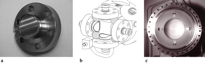
(a) Example of a button electrode from the CERN LHC. (b) Schematic of the full LHC button pick-up assembly for dual plane measurement using four electrodes. (c) Example of a stripline pick-up from the CERN-SPS
Fig. 8.60 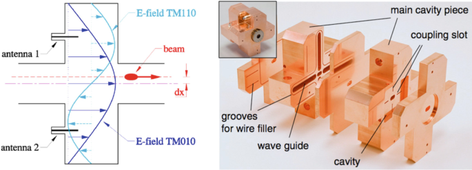
Principle and example of a cavity pick-up (ATF2, KEK, Japan)
A second type of electromagnetic monitor is the cavity pick-up (Fig. 8.60). These are constructed to exploit the fact that an off-centre beam excites a dipole mode (TM110) in the cavity, with the amplitude of excitation directly proportional to the off-axis displacement of the beam. This dipole mode has a slightly different frequency from the main monopole mode (TM010) of the cavity, which allows an excellent suppression of the intensity related signal. This in turn can lead to very good accuracy and nanometre scale resolution 121].
-
Resistive/Inductive
These monitors make direct use of the image current flowing on the wall of the vacuum chamber. A ceramic gap is used to force the image current through external resistors, in the case of the resistive (wall current) monitor, or through metallic rods fitted with transformers in the case of the inductive pick-up [122]. The position is calculated by comparing the output from suitably placed resistors or rods.
-
Magnetic
Such monitors are usually exploited for their relative insensitivity to stray particles. In this case the two electrodes are replaced by two loops orthogonal to the plane of measurement which couple to the magnetic field of the beam.


8.6.1.2 Beam Position Acquisition Systems
In order to extract an intensity independent position from all of these monitors a normalised difference signal needs to be obtained, i.e. a difference signal which is independent of the beam intensity [123]. In the case of the cavity this is simply done by dividing the output of the dipole (difference) cavity with that of a separate monopole (sum) cavity. In all the other cases one of the following methods is employed (A and B being the signal from each electrode):
-
Difference over sum (Δ/Σ)
The sum and difference are obtained either using a 0°/180° passive hybrid, a differential amplifier or calculated by software after digitising the signal from each electrode The resulting transfer function is highly linear with Normalised Position = (A−B)/(A+B).
-
Logarithmic ratio
The two input signals are converted into their logarithmic counterparts and subtracted. In practice this is done using logarithmic amplifiers followed by a differential amplifier. The transfer function is an S-shaped curve which becomes highly non-linear when exceeding 70% of the normalised aperture: Normalised Position = Log (A/B) = Log(A) − Log(B).
-
Amplitude to Phase or Time
The two input signals are converted into signals of equal amplitude but varying phase by combining them in a 90° passive hybrid. Normalised Position = φ = 2×arctan(A/B). The transfer function is again an S-shaped curve but does not diverge for large excursions. In addition, the gradient is larger around zero, making it more sensitive towards the middle of the pick-up.
The type of normalisation to be used will depend on the choice of processing electronics, which in turn depends on the type of measurements to be performed (single pass, single bunch, average orbit etc.). In all cases the non-linearity is taken into account by calibration circuits and correction algorithms. Common acquisition electronics include:
-
Multiplexed
Each electrode is multiplexed in turn onto the same, single acquisition electronics chain. This eliminates channel to channel variations, giving very good accuracy. However, since the switching is generally quite slow such an acquisition only tends to be used in circulating machines where the average position is of importance.
-
Sigma/Delta
A passive hybrid is generally used to produce sum (Σ) and difference (Δ) from opposite electrodes. The resulting signals are then directly digitised, or downmixed to lower frequency before digitisation using homodyne detection (self-mixing the signal) or heterodyne detection (external mixing using a clock related to the accelerator radio-frequency). Once digitised, the position is computed as K×Δ/Σ with K a scaling factor dependent on the pick-up geometry (typically close to ¼ of the aperture).
-
Individual Treatment
Each electrode is acquired separately but in parallel either by direct digitisation or logarithmic amplifiers. Position is calculated by difference over sum or logarithmic ratio normalisation by the central processing unit of the acquisition system.
-
Passive Normalisation
Such electronics convert the amplitude difference from opposite electrodes into a phase or time difference, which can then be detected using standard phase detection or time to digital conversion techniques. The position is extracted from this measurement using amplitude to phase or time normalisation as described above.
8.6.2 Beam Current and Intensity Measurement
The measurement of beam current or bunch intensity is one of the most basic measurements performed at any accelerator [124]. This is usually done by means of a Faraday Cup or Beam Current Transformer (BCT).
8.6.2.1 Faraday Cup
The Faraday cup technique relies on measuring the charge deposited in a metallic cup when intercepting the whole beam. This requires careful design, often using a bias voltage or magnetic field at the entrance of the cup, to avoid the secondary charges created by the interaction of the beam with the metal from escaping. They are usually used for relatively low current measurements due to problems related to the heat-load for higher intensity beams. Such devices act as an absolute calibration standard and are capable of providing fA resolution [125].
8.6.2.2 AC Beam Transformers
In order for a transformer to interact with the magnetic field of the beam it has to be placed over a ceramic gap in the vacuum chamber. The wall current accompanying the beam along the metallic wall of the vacuum chamber is deviated around the transformer using a low impedance radio-frequency bypass. A beam current, I B, can be considered as the primary winding of the transformer, with the output voltage from the secondary windings given by V α L dI B /dt, L being the transformer inductance. An ideal transformer would give a differentiated response, with the integrated charge being zero, which is not of much use as a measuring device. In reality the secondary windings of the transformer have some capacitance and are terminated by some finite resistance. This leads to signals that closely resemble the beam intensity distribution, with the added inconvenience of a DC offset due to the transformer droop. This DC offset can be corrected for either electronically or by software treatment of directly digitised data. Bandwidths from 200 Hz to 1 GHz are now available, using ferromagnetic cores wound with high permeability metal tape to avoid eddy currents. Such transformers are capable of resolving the charges contained within single short bunches, acquired either by direct digitisation or using fast integrator electronics. Resistive or inductive wall current monitors can also be used to provide such signals, but again require DC offset compensation [126].
8.6.2.3 DC Beam Transformers
In storage rings and accelerators with cycle times of several seconds a DC beam Current Transformer (DCCT) can be used to measure the total current. Such an instrument has a bandwidth that extends from a few kHz down to DC (hence its name) and was developed for the CERN-ISR (Intersecting Storage Rings), the first machine to sustain beams for hours [127].
A DC transformer is based on a pair of matched, toroidal, ferromagnetic cores, which are driven into saturation by a modulation current at frequencies of up to a few kHz. The principle of operation makes use of the hysteresis loop of the toroid. If an equal but opposite modulation current is applied to both cores with the beam not present, then the voltage induced in the detection windings on each core will be equal but opposite. When, however, there is a beam current present, the starting point in the hysteresis loop for zero modulation current is offset due to the static magnetic field generated by the beam current. Since the modulation is opposite in each toroid, the time spent in saturation will be different for the two branches of the hysteresis loop. This results in the generation of voltage pulses at twice the modulation frequency when the induced voltage in the detection windings on each core is combined. The demodulation of this signal gives a train of pulses, with the width of each pulse being a direct measure of the beam current, i.e. by how much the hysteresis curves are offset.
In the “zero flux detector” implementation of the DC beam transformer, the result of the demodulation is fed back through the pair of transformers by a compensating current loop (Fig. 8.61). Once the compensation current and the beam current are identical the net static magnetic field seen by the toroids is zero (hence zero flux) and the output from the demodulator is also zero. The beam current is then simply obtained by measuring the voltage produced by this compensation current across a known resistor. For modern DC transformers such a zero flux detector is combined with an AC transformer. The AC transformer is used to feedback on fast changes which are not compensated by the DC transformer and hence significantly increases the bandwidth of the system, allowing measurement from DC to a few MHz.

Schematic of a Modern DCCT. The two cores on the right form the “zero flux” DCCT, while the left hand core is an AC transformer that extends the bandwidth of the system to higher frequency
8.6.3 Diagnostics of Transverse Beam Motion
The instrumentation used to look at transverse beam motion is very important for the efficient operation of any circular accelerator [128]. There are three main parameters that can be measured using such diagnostics: the betatron tune, chromaticity and coupling.
8.6.3.1 Tune Measurement
All betatron tune measurements are based on measuring the characteristic frequency of the transverse motion of the beam. In the simplest case the beam is given a single kick using a powerful stripline or magnetic kicker and allowed to oscillate freely. A position pick-up is then used to measure the resulting beam motion, with the betatron tune being the frequency which has the highest amplitude response in the power density spectrum obtained using Fourier Transform techniques. If the detection technique is sufficiently sensitive (see e.g. [129, 130]) and there is enough external excitation from other sources such as ground motion then the method also gives useful information without any specific, additional beam excitation (Fig. 8.62).

Beam response to a single-turn kick excitation (top, left) and corresponding magnitude spectrum (top, right). Example of continuous tune measurement in the CERN Super Proton Synchrotron (left)
What is usually of more interest is to be able to track the tune evolution during the whole of the acceleration cycle. The simplest way of achieving this is to repeat the tune measurement at regular intervals, with the results displayed as a spectrograph. In order to minimise the frequency range over which power is put into the beam, a swept excitation frequency or “chirp excitation” is often used (so-called because if listened to at audio frequencies such a signal sounds like the chirp of a bird). The chirp range is set around the expected betatron tunes and the sweep time is determined depending on the requested time resolution and precision of the tune measurement. The advantage of this technique is that in addition to an amplitude response it also gives phase information. This makes it more sensitive than the single kick method and so allows smaller excitation amplitudes to be used.
To have a fully continuous measurement of the tune when no signal is visible due to external sources, a Phase Locked Loop (PLL) needs to be implemented. A voltage or numerically controlled oscillator (VCO or NCO) is used to put a sine wave excitation, Asin(ωt), on the beam. The beam response to this signal is then observed using a pick-up and will be of the form Bsin(ωt+ϕ), where ϕ is the phase difference between the excitation and the observed signal. A phase detector multiplies the excitation and observed signals together, giving a signal of the form ½ABcos(−ϕ) − ½ABcos(2ωt+ϕ) which has a DC component proportional to the cosine of the phase difference. This will therefore be zero when the phase difference is 90° and the amplitude response is a maximum, i.e. at the tune frequency. The aim of the PLL is to “lock-in” to this 90° phase difference between excitation and observed signal by correcting the VCO frequency until the DC component of the phase detector output is zero. Since the PLL will always try to maintain this 90° phase difference, the VCO frequency will track any tune changes, so giving a continuous tune measurement.
In practice things are not quite that simple. Many parameters have to be optimised in order to for the PLL to find, lock-in and subsequently track the tune peak. The beam spectra and dynamics also have to be well understood if the PLL is not to lock or jump to a spurious line, resonance, synchrotron sideband etc. In addition, for hadron machines, the continuous excitation will lead to some emittance blow-up. In order for this to be kept to a minimum the applied excitation has to be small and therefore the observation pick-up and following electronics very sensitive. This is less of a problem for lepton machines, where radiation damping takes care of any emittance blow-up caused by the excitation, making PLL systems much easier to implement on such machines.
8.6.3.2 Chromaticity Measurement
For any high energy synchrotron, the control of chromaticity is very important for beam stability and quality. If the chromaticity is of the wrong sign (positive below transition energy or negative above) then the beam quickly becomes unstable due to a head-tail instability. If the chromaticity is too large then the tune spread increases such that particles are inevitably lost as they hit resonance lines in tune space. The most common method of measuring the chromaticity of a circular machine is to measure the betatron tune as a function of the beam momentum and then to calculate the chromaticity from the resulting gradient. This is usually done by varying the RF frequency, keeping the magnetic field static. The equations of interest are:
where ΔQ is the change in tune, Δp/p the momentum spread (or relative change in momentum), ΔR/R the relative change in average radius, Δf/f the relative change in RF frequency and ξ the chromaticity. Please note that the chromaticity, ξ, is often expressed as Q' = Qξ, where Q is the total betatron tune including the integer part. A typical chromaticity measurement therefore consists of performing a tune measurement for several different RF frequency settings. What is usually measured is the average change in closed orbit, due to dispersion, from which the relative change in radius, and hence momentum change can be calculated. The chromaticity is then simply the measured tune change divided by the applied momentum change.
In order to obtain a continuous chromaticity measurement the technique of RF modulation can be combined with PLL tune measurement [131].
8.6.3.3 Coupling Measurement
The control of coupling (the degree to which horizontal and vertical betatron motion is linked) is also important for circular accelerators. Excessive coupling will make tune and chromaticity measurements almost impossible, as the information from both planes are mixed-up in the observed signal. A direct measure for the total coupling coefficient |C -| can be obtained by the “closest tune approach” method. Both betatron tunes are measured during a linear quadrupole power converter ramp which crosses the values of the horizontal and vertical tunes. Any coupling present in the machine will introduce a forbidden band through which the tune cannot cross, instead jumping from one side to the other. The width of this band is given by the total coupling coefficient |C -|.
In order to obtain a continuous measurement of coupling the PLL tune measurement can again be used, comparing the amplitude of the tune response in the plane of excitation with that of the other plane [132].
8.6.4 Beam Profile Measurements
Transverse beam distribution measurements are performed in all accelerators. As well as providing a direct measure of the beam quality, they can be used verify accelerator lattice functions and to calculate the emittance of particle beams. There are many ways to measure the beam size with the most commonly used techniques described in this section.
8.6.4.1 Secondary Emission Grids
Secondary Emission (SEM) Grids, also known as harps, consist of ribbons or wires which are placed in the beam [133]. See Fig. 8.63. As the beam intercepts the grid, secondary emission occurs leading to a current in each strip which is proportional to the beam intensity at that location. By measuring this current for all strips a beam profile is obtained. SEM-grids are the most widely used means to measure the density profile of beams in transfer lines. In addition, sets of three, properly spaced grids (i.e. with the right phase advance between monitors), allow a direct determination of the complete emittance ellipse. What makes them popular is their simple and robust construction, the fact that there is little doubt about the measured distribution, and their high sensitivity, in particular at low energies and for ions. At higher energies they can be considered semi-transparent. Amongst their drawbacks are the limited spatial resolution (difficult to get the wire spacing much below 0.25 mm) and the rather high cost for the mechanisms and electronics.

Secondary emission grid and its insertion mechanism
8.6.4.2 Scintillator and Optical Transition Radiation Screens
Scintillator screens have been used for nearly a century and are the simplest and most convincing device when one has to thread a beam through any accelerator. The modern versions used in accelerator instrumentation applications [134] are typically based on an activated inorganic ceramic or crystal structures, such as chromium activated alumina (Al2O3) or Cerium doped YAG (Y3Al5O12). These screens are directly inserted into the beam’s path and can stand high intensities and large amounts of integrated charge. In its simplest form a graticuled screen is observed using a TV-camera. It can deliver a wealth of information to the eye of an experienced observer, but precautions need to be taken into account to extract quantitative measurements. Much can be done about that with modern means of rapid image treatment, but questions concerning the linearity of these screens at high beam densities remain.
Optical Transition Radiation (OTR) [135] screens are a cheap substitute for scintillator screens. OTR radiation is generated when a charged-particle beam transits the interface between two media with different dielectric constants (e.g. vacuum to metal or vice versa) [136]. Since this is a surface phenomenon, the screens can be made of very thin foils which reduces beam scattering and minimises heat deposition. The radiation produced when the beam enters the foil is emitted in a narrow cone around the angle of reflection for backward (vacuum to metal) OTR so that if the foil is placed at 45° to the beam direction, the radiation produced is at 90° to the beam direction. In addition, forward OTR (metal to vacuum) is also produced around the beam direction when the beam exits the foil. The angular distribution of the emitted radiation has a central hole and a peak located at 1/γ. The higher the value of γ the sharper the peaks and the more light can be collected, which is why OTR is generally suited to lepton or high energy hadron machines. The imaging can again be performed using simple optics followed by a CCD camera. See Fig. 8.64. Recent studies have demonstrated that OTR imaging systems are capable of measuring a beam size below one micron [137, 138]. A non-invasive alternative to OTR screens has been developed using diffraction radiation from slits [139], which has also demonstrated good performance [140].

(Left) Combined OTR and scintillator screen mechanism showing chamber in the out position and (bottom) an example of images obtained during the very first injection into the LHC
8.6.4.3 Wire Scanners
Of all the instruments used for measuring the emittance of circulating beams, wire-scanners are considered to be the most trustworthy. They come in two different types; rotative and linear. Rotative wire scanners can reach speeds of up to 20 ms−1 and consist of a thin wire (some tens of microns in diameter) mounted on a fork which is attached to a rotating motor, while linear scanners use motors which push/pull the wire across the beam. There are two ways of obtaining a beam profile with wire scanners; by measuring the secondary emission current in the wire as a function of wire position (similar to SEM-grid acquisition) or by measuring the flux of secondary particles created as the beam interacts with the wire. This latter technique is often used for high intensities, where the heating of the wire produces thermal emission which falsifies the secondary emission results. It relies on the use of radiation detectors, typically scintillators followed by photo-multipliers, placed downstream of the wire scanner to detect the γ-radiation and secondary particles produced when the wire intercepts the beam. To make the flux collected independent of the wire position may require the summation of the signals from two or more detectors positioned around the beam chamber. Fast wire scanners are nearly non-destructive over a wide range of energies. Their spatial resolution can reach the micrometer range [141] and, with fast gated electronics, the profiles of individual bunches can be observed. Their great sensitivity also allows them to be used for the study of beam halo.
For H− and lepton accelerators the wire can be replaced by a laser beam, with the detection of stripped electrons [142] or Compton scattered [143] electrons respectively. This technique is ideally suited to high power machines, where a wire would not survive, or to machines where the transverse beam size is extremely small requiring a very thin ‘wire’ which is obtained by tightly focussing the laser beam.
8.6.4.4 Residual Gas and Luminescence Monitors
Rest gas monitors are used in many high energy accelerators in order to reconstruct transverse beam distributions [144]. The signal results from the collection of either the ions or the electrons produced by the beam ionising the small amount of residual gas in the vacuum chamber. These ions or electrons are accelerated using a bias voltage of several kilovolts and typically collected on a micro channel plate (MCP). The avalanche of electrons produced by the MCP are then collected on strip detectors or hit a phosphor screen to give an image of the beam profile that can be monitored using a CCD camera. Due to their rigidity, ions are less sensitive to the distorting effects of the space charge from the circulating beam, but their slow drift time, even with high bias voltages, means that they spend a long time in this beam field, making it difficult to analyse beam dimensions smaller than one millimetre. However, in order to use electrons to produce an image, a transverse magnetic field needs to be added around which the electrons spiral on their way to the MCP. This eliminates, to a large extent, the space charge effects of the beam and allows sharper images to be produced than with ions. This additional magnetic field is also seen by the beam and has to be compensated by two corrector magnets either side of the ionisation profile monitor. Direct detection of ionized particles using in-vacuum pixel sensors has recently been demonstrated as an alternative to MCP detection [145], providing a more sensitive monitor and eliminating the ageing effects associated with micro channel plates.
Luminescence monitors [144] also rely on the interaction of the beam with a gas in the vacuum chamber. In this case electrons are excited from the ground state to a higher energy level by the passing beam. Once the beam has passed the electrons return to the ground state and emit photons. In the case of nitrogen the dominant photon wavelength is 391.3 nm, corresponding to light at the lower end of the visible range, for which many detectors are available. In general, the residual gas alone does not produce enough photons for accurate imaging and hence a local pressure bump is usually created by injecting a small amount of additional gas to enhance the photon production.
Most users consider both the residual gas ionisation and luminescence profile monitors to be semi-quantitative and not to be relied upon for absolute emittance measurements, even after calibration against some other instrument such as a wire scanner. Their virtual transparency for the beam, however, makes them useful for the continuous on-line tracking of beam size.
8.6.4.5 Synchrotron Radiation Monitors
Synchrotron radiation monitors [146] are limited to highly relativistic particles and offer a completely non-destructive and continuous measurement of the 2-dimensional density distribution of the beam. These monitors make use of the light produced when highly relativistic particles are deflected by a magnetic field. They are therefore usually positioned to make use of parasitic light produced by a dipole magnet in the machine or behind a purpose built “undulator” magnet in which the beam is deflected several times to enhance the photon emission.
The most common way of measuring the beam size with synchrotron radiation is to directly image the extracted light using traditional optics and a camera. The spatial resolution for such systems is usually limited by diffraction and depth-of-field effects which can be overcome using interferometers [147]. If the beam is sufficiently relativistic then the photon emission extends into the hard X-ray region of the spectrum and X-ray detectors can be used [148], for which diffraction effects become less important.
8.6.5 Beam Loss Monitoring
Beam loss monitors (BLMs) have three main uses in particle accelerators: Damage prevention, diagnostics and machine optimisation [149]. The job of the BLM system is to establish the number of lost particles at a certain position within a specified time interval. Most BLM systems are mounted outside the vacuum chamber, so that the detector observes the shower caused by the lost particles interacting in the vacuum chamber walls or in the materials of the magnets. The number of detected particles and the signal from the BLM should be proportional to the number of lost particles. This proportionality depends on the position of the BLM with respect to the beam, the type of lost particles and the intervening material. It also, however, depends on the momentum of the lost particles, which may vary by a large amount during the acceleration cycle. One has to distinguish between two types of losses; fast losses, where a large amount of beam is lost in a short time (for circular machines) or distance (for LINACs and transport lines) and slow losses, where partial beam loss occurs over some time or distance. In storage-rings, the lifetime is defined by slow losses. Superconducting accelerators use the BLM system to prevent beam loss induced quenches. The fact that BLM systems have to cover both of these cases means that they are often required to function over a very large dynamic range, typically in the region of 104 to 106. BLMs can be classed into two main families: global—containing a few long detectors covering most of the accelerator; distributed—with many units of relatively small active area.
8.6.5.1 Global BLM Systems
The first global system was proposed by Panowsky for SLAC in 1963 [150] and was composed of a 3.5 km hollow coaxial cable filled with Ar (95%) + CO2 (5%), mounted on the ceiling of the LINAC, about 2 m from the beam. When a beam loss occurs the secondary particles produced traverse the monitor and induce an electrical signal which propagates to both ends of the cable. Position sensitivity is achieved by comparing the time delay between the direct pulse from one end and the reflected pulse from the other. The time resolution achievable with such systems is about 30 ns (~8 m), which can be reduced to about 5 ns by using shorter cables. This principle of space resolution works for relativistic linear accelerators and transport lines with a bunch train much shorter than the machine. For particles travelling significantly slower than the signal in the cable the resolution of multiple hits in the cable becomes difficult. In this case, and for circular machines, it is necessary to split the cable. Each segment has to be read out separately, with a spatial resolution which becomes approximately equal to their length. A similar measurement can these days be achieved using Cherenkov or scintillation light created in long optical fibres [151]. The fast response of the Cherenkov signal is detected using photomultipliers at the ends of the fibre, allowing a longitudinal position resolution of 20cm to be achieved.
8.6.5.2 Distributed BLM Systems
By far the most common, distributed BLM systems are comprised of many individual beam loss monitors located throughout the accelerator, each acquired in parallel. The active medium in these systems is tailored to the type of loss to be measured. Ionisation chambers are commonly used due to their robustness and large dynamic range (see e.g. [152]). The chamber provides some medium with which the secondary particles created by the beam loss can interact, typically a gas such as nitrogen or argon. This interaction produces electron-ion pairs that are collected by a series of high voltage gaps along the length of the chamber. The resulting current is then measured and is proportional to the beam loss at the location of the monitor.
The drawback of the ionisation chamber is its relatively slow response time, dominated by the drift velocity of the ions created during a beam loss. In cases where a fast response is required scintillation counters are often employed. These come in plastic or liquid form and are read-out using a photomultiplier. The disadvantages of these systems are the susceptibility of plastic scintillators to radiation damage and long term drift of photomultiplier gain. It is also possible to directly use the photomultiplier as a detector by replacing the photocathode with an aluminium foil that works as a secondary electron emitter when irradiated. Known as an Aluminum Cathode Electron Multiplier (ACEM) it gives response times in the nanosecond regime [153]. Diamond detectors, consisting of a biased monocrystalline or polycrystalline diamond wafer with an active area of a few cm2, have also recently been demonstrated to give nanosecond response times while being relatively radiation resistant [154].
In order to distinguish beam losses in accelerators where there are sources of background ionising radiation such as X-rays or synchrotron radiation, Cherenkov or PIN photodiode detectors can be used. Cherenkov detectors are useful as the threshold for light production is above the typical Compton-electron energies produced by such background radiation, while back to back PIN photodiodes can be used to distinguish between the hadronic shower created by beam losses and synchrotron radiation [155]. In the latter case only the charged particles will interact with both photodiodes, giving a coincidence signal, with the photons absorbed by the first diode. In contrast to the charge detection of most other BLM systems, PIN photodiode detection depends on counting coincidences, with the count rate proportional to the loss rate so long as the number of overlapping coincidences is small.
8.6.6 Short Bunch Length Diagnostics
Recent developments for Free Electron Laser (FEL) accelerators and studies for linear colliders in the TeV range are driving the typical bunch length of accelerated lepton beams down to the 10–100 femtosecond level. To measure the longitudinal behaviour of such beams is not trivial and a lot research has been carried out over the last decade to develop instruments that allow their characterisation. They broadly fall into three categories: direct beam observation; coherent radiation techniques; radio-frequency and electro-optic sampling techniques.
8.6.6.1 Direct Beam Observation
Direct Beam Observation, as its name suggests, relies on the direct measurement of longitudinal beam structure by means of fast detectors. Wall Current Monitors followed by fast sampling oscilloscopes are able to probe time structures down to well below the nanosecond, while streak cameras can reach some 200 femtoseconds [156]. The latter relies on analysing an optical replica of the longitudinal bunch distribution obtained by means of synchrotron, transition, diffraction or Cherenkov radiation.
8.6.6.2 Coherent Radiation
For wavelengths shorter than the bunch length, the particles within the bunch radiate incoherently, with the power emitted proportional to the number of particles. However, for wavelengths equal to or longer than the bunch length, the particles emit radiation in a coherent way with the emitted power dependent on the bunch length and scaling as the square of the number of particles.
where S(ω) represents the radiation spectrum, S p(ω) the single particle spectrum, N the number of particles and F(ω) the longitudinal bunch form factor, which depends on the longitudinal particle distribution ρ(s).
Measuring the power spectrum therefore allows the form factor to be calculated from which an indirect estimate of the bunch length is possible. This method is relatively simple to implement and has already demonstrated its capacity for the measurement of extremely short bunches [157].
8.6.6.3 Radio-Frequency and Electro-optic Sampling Techniques
These techniques rely on encoding the longitudinal bunch length information into spatial or optical information. Radio-frequency manipulation makes use of a transverse RF deflecting cavity [158] to kick the head of the bunch in one direction and the tail of the bunch in the opposite direction. By measuring the transverse beam size downstream, it is then possible to reconstruct the longitudinal bunch profile. This technique is the standard method for measurement of femtosecond bunches, with the drawbacks being its destructive nature and cost.

Electro-optic sampling techniques for the measurement of short bunch lengths
Electro-optic sampling [159] (Fig. 8.65) is an alternative to the RF technique and relies on converting the coulomb field of the bunch into an optical intensity variation by means of an electro-optic crystal. The crystal is placed close to the beam so that the charged particles in the bunch induce a polarization change of a laser beam passing through the crystal at the same time. Three main types of encoding are in common use; spectral, temporal and spatial. In spectral decoding the beam passes the electro-optic crystal at the same time as a chirped wavelength laser pulse. The longitudinal distribution of the bunch is hence encoded as an optical power variation at different wavelengths in the chirped laser pulse. A spectrometer is used to separate out the wavelengths and so reconstruct the longitudinal profile. Temporal decoding [160], works in much the same way as spectral decoding, with the spectrometer replaced by a non-linear crystal. A femtosecond laser pulse is mixed with the chirped laser pulse in this crystal to produce a frequency doubled replica of the longitudinal distribution. Spectral encoding can characterise bunch distributions down to the picoseconds level, while temporal encoding works down to some 100 femtoseconds. Spatial decoding [161] uses a short laser pulse that crosses the crystal at an angle such that when it interferes with the beam signal, the temporal profile of the electron bunch is encoded onto the transverse profile of the laser, i.e. mapping time into space.
Such techniques all rely on the use of very short laser pulses and precise laser to beam synchronization.
8.7 Injection and Extraction Related Hardware: Kickers and Septa
This chapter describes the main hardware elements involved in single-turn injection and fast extraction, as well as resonant slow extraction: fast pulsed systems (kickers) and magnetic and electrostatic septa. For a description of the beam processes involved reference is made to Sect. 6.3. For space reasons other associated components, such as stripping foils used for multi-turn injection, injection and extraction related protection systems, or specific beam instrumentation, are not discussed here. For certain of these components information can be found in the corresponding chapters of this volume.
Injection and extraction regions are particularly challenging areas in accelerators in several respects. The space allocated for these parts, which are usually located in straight sections, is naturally rather limited so that the space available for bending sections (in the case of a circular machine) or accelerating structures (in the case of a linear accelerator) can be maximized, and with it the achievable energy for a given circumference or length of the accelerator. As a result injection and extraction related elements are often required to be as physically short and electrically or magnetically strong as technically feasible (yet remaining reasonable in cost). Although magnetic kickers and septa are dipole magnets, following the same principles as ordinary bending elements, they have very distinct features and must often fulfil conflicting design requirements. They are typically purpose-built single elements or only produced in a small series. Many of these elements are installed under vacuum, with the resulting implications.
Figure 8.66 shows an example of fast single-turn injection in one plane [162, 163]. The injected beam passes through the homogeneous field region (aperture) of the septum: circulating beam is in the field-free region. The septum deflects the injected beam onto the closed orbit at the centre of the kicker magnet; the kicker magnet compensates the remaining angle. The septum and kicker are either side of a quadrupole (defocusing in the injection plane) which provides some of the required deflection and minimizes the required strength of the kicker magnet.

Fast single-turn injection in one plane
Magnetic septa usually have high current densities (in the order of 100 A/mm2); a short interruption in the cooling can lead to their destruction. Electrostatic septa are operated with very high fields and must also cope with the heat load from the impinging beam. To reduce the particle losses septa (coils, or foils/wires in case of electrostatic septa) must be as thin as possible; nevertheless, the characteristics of the beam processes involved mean that septa are usually among the most radioactive parts of an accelerator, together with collimators and dumps. This has to be taken into account during the design, for example, it must be possible to quickly assemble and release electrical, water and vacuum connections.
The rise time of the field produced by the kicker magnets must be very short (ranging from several tens of μs down to several ns), while the requirements for low ripple and good reproducibility of the flat-top amplitude are stringent (at least considering the pulse-type excitation). Redundancy can also be an important design criterion: if one of the devices fails the remaining devices should be sufficient, in combination with special protection elements, to handle the beam safely. For single-turn injection or extraction there is only one action on the beam and the timing needs to be precisely set up; although it may be feasible to compensate for small, non-ideal, deflection of the first and last bunches of a train [164], significant online corrections are not possible. Applications are often safety critical (beam abort systems) and imminent failures must be recognized in real time.
8.7.1 Fast Pulsed Systems (Kickers)
Apart from their use for injection and extraction purposes specific kickers are also used to excite the beam, for instance to measure the tune or probe the machine aperture. Kicker magnet yokes are frequently made out of NiZn ferrite because of its relatively high resistivity and magnetic permeability: with the NiZn ferrite field rise can track current rise to within ~1 ns [165], while slower kickers can use laminated steel yokes. Fast rise times are particularly required in smaller machines to optimize the filling factor (amount of beam which can be injected). Useable pulse durations are in the range of a few 100 ns to 100 μs (case of the CERN LHC beam dump kicker which must empty the whole 27 km circumference at once; here the fall time is not important as all beam is anyway extracted after one turn). Even faster rise times, in the range of a few ns, can be achieved with yoke-free stripline kickers, where the field is created by a pulse running along two longitudinal electrodes [166, 167].
The main design options for kicker systems include the type of magnet (“travelling wave” (also known as “transmission line”) or “lumped inductance”), the installation of the magnet in- or outside of the machine vacuum, the type of aperture (window-frame or C-core), and the type of termination (impedance-matched or short-circuited) [162]. The actual choice depends on the demands and constraints of the application, but is also impacted by cost considerations. Applications where a considerable number of bunches must be placed at a precise position on the circumference of an accelerator, without disturbing the already circulating bunches, or where only a part of the circulating beam needs to be extracted, requires kickers with fast rise and fall time. Low flat-top ripple reduces the injection oscillations which could lead to emittance blow-up (in hadron machines), and ensures constant deflection angle for a train of extracted bunches. To achieve fast rise and fall times and low flat-top ripple, quasi-rectangular pulses are applied to “transmission line” kicker magnets. For space reasons most of the discussion below will be devoted to such systems.

Simplified block diagram of a typical transmission line kicker system
A simplified block diagram of the power circuit is given in Fig. 8.67. Shortly prior to the required kicker pulse a resonant charging power supply (RCPS) charges either a high voltage coaxial cable (also known as a Pulse Forming Line (PFL)) or a Pulse Forming Network (PFN); the choice between a PFL and a PFN is discussed below. At the appropriate time the main switch (thyratron or semiconductor) is turned on (closed) and the pulse current is sent through a coaxial transmission line into the kicker magnet. In the schematic of Fig. 8.67, once the current pulse has passed through the magnet the energy is absorbed in a terminating resistor. If for any reason the pulse current must not be sent to the kicker magnet (for instance if the accelerator turns out to be no longer ready to receive beam or the kicker system exhibits an internal fault, e.g. a charging voltage not matching the beam energy), the dump switch is turned on and the PFN is thus discharged. The dump switch is also turned on when the pulse duration, in the kicker magnet, needs to be reduced. An additional “clipper switch” can be used to connect the magnet side of the PFN to ground in order to improve the fall time. The main components of the electrical circuit are all matched to a characteristic impedance Z (typically in the range of a few Ohms to a few tens of Ohms) to avoid unwanted reflections and thus distortions of the pulse shape. The interplay of the different components is therefore important and a carefully chosen set of parameters and a coherent design are required to achieve optimum performance. Computer aided design tools (electric circuit simulation and finite element analysis software) are used extensively to predict and verify the performance achieved by the hardware, or to study how an existing system can be improved [162]. The main components of a kicker system are presented in more detail below.
8.7.1.1 Kicker Magnets
A transmission line magnet consists of typically between 5 and 30 cells (Fig. 8.68) to approximate the behaviour of a coaxial cable. The cells consist of either a sequence of metallic plates which are alternately connected to the high voltage conductor and ground, thus forming capacitors, or commercial capacitors. Ferrite cores are sandwiched between the high voltage plates (Fig. 8.69).

Simplified equivalent electric circuit of a transmission line kicker magnet

Cut-away of a transmission line kicker magnet
After general considerations, such as available space, deflection angle, rise time, flat-top ripple, and fault tolerance, the system design usually commences with the choice of the charging voltage (V) and the characteristic impedance (Z) of the system. The impedance is given by Z = (L c/C c)1/2, where L c and C c are the inductance and capacitance of a cell, respectively (Fig. 8.68). The choice of Z depends on the required field rise time and the space available. The field rise time is given approximately by the sum of the current pulse rise time, at the terminating resistor, and the fill time of the magnet [162]. The fill time (t m) of a kicker magnet, terminated in its characteristic impedance, is given by t m = L m/Z; to achieve a short fill time the series inductance of the magnet, L m, should be small and the impedance rather high. In addition high impedance provides for a relatively high cut-off frequency [162] which in turn helps achieve a low flat-top ripple. In the case of a C-core kicker magnet the high voltage conductor usually consists of a single straight bar (single turn) which helps to ensure the low inductance. In practice impedances up to that of commercially available coaxial high voltage cables are used (50 Ω), within the boundaries dictated by the available length for the kicker magnets and the chosen PFN voltage. The lower the impedance needs to be the greater must be the cell capacitance. In magnets using vacuum as dielectric, high cell capacitance requires that either the plate surfaces are very large (which would be impractical for space reasons) or the separation between high voltage and ground plates is small (however the distance must not be made so small so as to risk electrical breakdown). Therefore in some cases capacitor media with higher permittivity must be used, e.g. ceramic capacitors, as for instance is done for the LHC injection kickers.
A design where the whole kicker magnet is under vacuum allows for the minimum size of magnetic aperture; for out-of-vacuum magnets the magnetic aperture must also enclose a vacuum chamber. For a larger aperture the current must be increased to ensure that, for a given impedance, the same magnetic flux is achieved, which in turn implies an increase of the PFN voltage [162]. Hence, for a given current, under-vacuum magnets can be of a shorter length than the equivalent out-of-vacuum magnet, but also have some disadvantages. The magnet materials must be compatible with the vacuum requirements and the whole construction must allow for bake-out and resulting thermal expansion. In addition a vacuum tank and pumps are required, and the repair in case of magnet or vacuum equipment failures is usually very time consuming.
The termination of the kicker magnet with a resistor (Fig. 8.67) avoids unwanted reflections and ensures a fast filling time of the magnet. The resistor is usually formed by a stack of high power ceramic-carbon resistor disks housed in a coaxial metallic enclosure, which is the return path of the current, to minimize the inductance and thus allow good matching over a wide range of frequencies. For cooling and insulation purposes the resistors are usually immersed in oil. Where available length for the kicker magnet has priority over rise time, a short circuit at the pulse output end of the magnet has the advantage of doubling the kick strength, for a given PFN voltage and system impedance. However the fill time of the magnet is also doubled; to establish full field in the magnet the pulse has to travel to the magnet output and then reflect back to the driven end of the magnet. In addition, for a magnet terminated in a short-circuit, during the field pulse the magnet also experiences both polarities of voltage [162].
8.7.1.2 Beam Coupling Impedance
Kicker magnets with ferrite or laminated steel yokes, directly exposed to the beam, can contribute a major fraction of the longitudinal and transverse beam coupling impedance of a machine [168]. The passage of the beam, without providing an appropriate path for the beam image current, can also cause resonances within the volume of the tank and lead to higher order mode losses. Since these effects can results in beam instabilities their reduction is becoming increasingly important with rising beam intensity. Electromagnetic coupling with high-intensity beams also leads to heating of the ferrites, sometimes beyond their Curie temperature.
Where needed and possible these issues are being addressed in existing applications by various retrofitting techniques, thus avoiding a costly redesign of the whole kicker system and possible implicit layout changes. The kicker magnet vacuum tank can be shielded from the beam by incorporating metallic transition pieces between the tank flanges and the kicker magnet [169] and between subsequent magnet modules in a common tank, thus minimising changes in aperture dimensions and avoiding some resonances.
To reduce the temperature rise of the ferrites, due to beam induced heating, indirect water cooling has been implemented with electrically insulating but thermally conducting Aluminium-Nitride plates in contact with the ferrites [170]. Particular precautions must be taken here because of the presence of the high voltage. To reduce the coupling of the beam with the ferrite yoke, without loss of aperture, two comb structures of silver paint stripes can be serigraphed onto a ferrite (Fig. 8.70, left) [171]. Each of the two sets of stripes is connected to a high voltage plate; the capacitive coupling between the two sets of stripes, which is enhanced by the permittivity of the ferrite, provides the path for the beam image current, without creating eddy current loops which would adversely impact the field rise time. Nevertheless the overlapping length of the two serigraphed combs should be optimized to avoid resonances at undesirable frequencies [172]. The serigraphy technique is less attractive for short cells because of both high voltage breakdown issues and the relatively small capacitive coupling between the two sets of stripes.

Serigraphed ferrite yoke of the CERN SPS fast extraction kickers (left); ceramic tube with wires forming the beam screen of the LHC injection kickers (right)
In new designs, where the beam impedance is taken into account from the beginning of the design, or where the available aperture permits, a proper beam screen can be inserted between the magnet yoke and the beam. In the LHC injection kickers a 3 m long ceramic tube serves as support for up to 24 Nickel-Chrome (80/20) wires lodged in grooves around its inner circumference (Fig. 8.70, right). The tube also provides insulation between the wires and the ferrites and high voltage plates, but has no vacuum function. On one end the wires are directly connected to the beam pipe, on the other end through a capacitive coupling with a grounded metallization on the outside of the tube [173]. The LHC extraction kicker magnets, which have a rise time of approximately 3 μs, use a 1.4 m long ceramic vacuum chamber with a 3 μm thin uniform Ti layer on the inside which acts as beam screen [174]. To note that beam screening techniques have equally to be compatible with the particular demands from ultra-high vacuum, nearby high voltage and acceptably low secondary electron yield [175].
For certain applications, e.g. beam extraction, the problem of beam impedance and screening can be diminished or to some extent circumvented if the beam circulates most of the time outside of the kicker, and is only bumped into the magnetic aperture of an open C-core kicker shortly (few ms) before the kicker is used [176]. The advantage of such a configuration is that the kicker aperture can be smaller, because of the beam shrinkage during acceleration, than if the beam passes through its aperture right from injection. However the smaller aperture may increase beam coupling impedance again; detailed studies are required to find the best trade-off.
8.7.1.3 Pulse Generation and Forming
The simplest pulse forming circuit consists of a coaxial cable (a pulse forming line, PFL) charged to twice the required pulse voltage. A PFL provides fast and low-ripple pulses but requires low dispersion and attenuation, especially for longer pulses, to keep droop and “cable tail” within specification. Since semiconductor materials in the cable (used to improve the breakdown voltage) increase the attenuation and dispersion, SF6 pressurized polyethylene (PE) cables have historically been used for PFL voltages above 50 kV. The required length and cost of PFL cable, as well as the attenuation and dispersion, limits the practical application to pulse durations of less than approximately 3 μs.
Where long pulses with low droop are required, a PFN is used which acts as artificial coaxial cable. The PFN consists of a series of “cells” forming a delay line. There are many configurations for PFNs [177] but a commonly used design is where each cell consists of a series inductor (sometimes with a parallel damping resistor) and a capacitor connected to ground (Fig. 8.71, left). The precision of the mechanical and electrical dimensions is important for a good pulse shape, i.e. short rise and fall times with low over- and undershoot, and low ripple. To preserve the precise inductance and to avoid time consuming adjustment by hand, longer coils are often wound onto an insulating support (Fig. 8.71, right) [178]. To obtain good matching and thus low ripple, two parallel lines can be used (Fig. 8.71): in addition, to compensate for conduction losses along the coil, the values of the capacitors are selected prior to assembly. The first cell and last cell of a PFN are mechanically adjustable, to allow catering for as-built imperfections which cannot be simulated with precision. The whole assembly is normally immersed in a dielectric liquid (polydimethylsiloxane or ester oil) which permits a more compact design than with air insulation, and which serves also as coolant.

PFN of the LHC injection kickers, consisting of two parallel 10 Ohm lines
Prior to turning on the main switch, to send the pulse to the kicker magnet, the PFN is charged to the voltage V. The charging components are usually connected at the dump switch end of the PFN (Fig. 8.67). When the main switch closes a pulse with amplitude of V/2 is sent through the transmission line to the kicker magnet and a voltage pulse of −V/2 propagates from the main switch end of the PFN towards the dump switch end. If the kicker magnet is terminated in its own characteristic impedance there is no reflection of the pulse which propagated through the magnet. However if the kicker magnet is short circuited at its output the pulse which propagated through the kicker magnet is reflected and travels backwards through the magnet, doubling the current and hence the field in the magnet; the fill time is in this case also increased by a factor 2.
8.7.1.4 Power Switching
Various technologies are used for power switching [177]. Thyratrons are still commonly used for fast, high power, switching applications. These deuterium filled gas tubes are characterized by a short turn-on time, high rate of rise of current and generally good reliability. They need however careful tuning and supervision of parameters such as reservoir voltage and grid bias voltages, as well as requiring occasional HV conditioning, to ensure optimum performance. Thyratron faults include failure to become conducting when required (so called “missing” pulses), or on the contrary becoming conducting before being triggered (so called “erratic” turn-on). High power thyratrons are also relatively expensive (up to several 10 k$ each) and have a limited lifetime which is strongly determined by the conducted charge (typically several 100 thousand pulses for very high current and long duration (tens of μs) pulses, to 100 million pulses for lower current and shorter pulses). To lower the risk of erratic turn-on the anode-cathode voltage is only applied to the thyratron a short time (typically few ms) before the kick is required. Although not many companies produce thyratrons anymore they are still widely used in accelerators.
For many years high power semiconductors have been used as switches in those kicker applications which do not require the high rate of rise of current of thyratrons. Semiconductors have the advantage of requiring little or no maintenance in comparison with gas tubes and they have a less critical dependence on the anode-cathode voltage, but generally have a lower rate of rise of current rating. An example where these switches are preferred are the LHC extraction (dump) kickers: the associated PFNs need to be charged over hours and the switches must therefore withstand the high voltage over extended periods without erratic turn-on. Semiconductors used for power switching in kicker systems include GTOs (Gate Turn-off Thyristors, which have been improved for fast switch-on; they are also called Fast High Current Thyristors (FHCTs)), IGBTs (Insulated Gate Bipolar Transistors), and MOSFETs (Metal-Oxide Semiconductor Field-Effect Transistors).
Although in principle semiconductors require no maintenance and have a very long lifetime when used in normal conditions, their application in accelerators is not completely straightforward. Since the typical breakdown voltage of a representative GTO is in the order of a few kV, the high voltages used in kicker systems requires the assembly of the semiconductors in series stacks (in practice up to 10–15 per stack, including redundancy) (Fig. 8.72). The distribution of the total voltage within the stack of series GTOs and the synchronous injection of a sufficiently high trigger current into the gates are important, to avoid excessive voltage across individual GTOs which could lead to unwanted conduction of the whole stack (“erratic”) or destruction of the power semiconductors. It is noteworthy that such assemblies are often operated near or even beyond their normal specification limits; this is to achieve suitable high current with adequately fast rise time. In areas with a high background radiation (either from activated ambient materials or from beam losses) the radiation effects can be cumulative, with relatively slow deterioration of semiconductor performance, and/or sudden malfunction or failure [179]. Protection against particle-triggered breakdowns can be important. For installations in which the turn-on delay is critical, temperature stabilization of the semiconductors (usually through cooling of the surrounding air) is also an issue. High power GTOs used for the LHC extraction kicker systems (Fig. 8.72) have turn-on delay times in the order of 300 ns, a hold-off voltage of 2.5 kV per GTO for d.c. operation, a current rate of rise capability of 20 kA/μs, and conduct a current with an amplitude of 30 kA.

Semiconductor switch stack of the LHC extraction kickers, together with voltage grading networks and gate trigger transformer
To provide redundancy in critical applications, two switches can be installed in parallel for each pulse generator, as for example in the LHC extraction kickers [174]. It should be noted, however, that putting switches in parallel has the disadvantage of increasing the risk of unwanted erratic turn-on. Other switch configurations include for example an ignitron in parallel with a thyratron, where the faster thyratron ensures the rapid and precise start of the pulse while the sturdier but somewhat slower ignitron takes over the bulk of the current [180]. Ignitrons are being phased-out from existing applications due to their mercury content, and resulting safety and environmental risk.
Topologies such as the inductive adder [181,182,183] and Marx generator [184, 185], utilizing fast and high-voltage semiconductor switches such as MOSFETs, are being actively pursued by CERN as possible alternatives to both thyratron and PFL technologies. The inductive adder and Marx generator use the series and parallel connection of power semiconductor switches to achieve high pulse power designs. The required energy is stored in capacitors. The MOSFET semiconductor switches have the ability to both turn on and turn off the current pulse.
Other types of switches for particular applications include so called “pseudo spark gaps”, fast high-voltage MOSFETS and Fast Ionisation Dynistors (FID, also called Fast ionization Devices) [162]. With advances in semiconductor technology new, interesting, types of devices or switches with improved characteristics are expected to become commercially available.
8.7.1.5 Other Types of Circuits
In applications where only a few bunches need to be injected or extracted (e.g. LEP), fast deflection is most economically achieved by an oscillation system using half-sine wave pulses, where a capacitor is discharged into a purely inductive magnet terminated in a short circuit [186]. In this case no particular PFN is needed and the magnet does not need to be fitted with matching capacitors, permitting important economies. The charging voltage is half that for a travelling wave kicker system, with the same magnetic parameters, which often allows working with more economic air insulation in the pulse generator.
Capacitive discharge systems complemented by free-wheel circuits are mainly used for applications such as beam abort systems where a fast rise of the magnet pulse is required which can be followed by a long exponential decay (since all beam has been dumped after one turn), while the requirements of the flat-top are not very stringent. This is the case for instance for the LHC extraction kickers [174]. Here a capacitor is discharged into an inductive magnet with a stack of diodes in parallel. During the sinusoidal rise of the current the diodes are non-conducting, but when the magnet current pulse starts to reduce in magnitude the diodes conduct and the magnet current free-wheels in the low impedance circuit.
Where very fast rise times are required (order of few ns) stripline kickers are used [166, 167, 187]. These consist essentially of electrodes parallel to the beam direction, and contain no magnetic material. The deflection is provided by the electric and magnetic field between the plates. Generators with fast semiconductor (MOSFET) switches are typically used and sub-nanosecond jitter can be achieved. For an ultra-relativistic beam, the beam is deflected only if it is travelling from the terminated to the driven end of the striplines [188]. A schematic view of a stripline kicker system, for the tail clipper of the CTF3 facility, is given in Fig. 8.73.

Schematic view of a stripline kicker system
8.7.1.6 Electronics and Controls
The electronics and controls for a fast pulsed system is an important, complex and voluminous part of the overall system. They must be designed from the outset together with the power circuit. Typically they comprise systems for synchronization with the accelerators (mainly the radiofrequency and general timing system), systems to generate and distribute the timing across the system (including fine delays), and power triggers to drive the high voltage switches. A beam energy tracking system checks that the charging PFN/PFL voltage corresponds to the present energy of the accelerator. Fast interlocks, waveform acquisition and analysis hardware and software, as well as comprehensive software to monitor, follow-up and document the performance of the overall system complete the installation.
8.7.2 Electrostatic and Magnetic Septa
A septum, either electrostatic or magnetic, constitutes the separation between an area of ideally zero field, which is traversed by the circulating beam, from an area with high field in which the injected or extracted beam experiences a deflection. The septum should be as thin as possible to reduce particle losses and thus irradiation of the septum and the surroundings. If used in combination with a kicker (case of single-turn injection or extraction, Fig. 8.66) it serves also to keep the strength requirements for the kicker at an affordable level. Since the beam passes only once through the high field area of a septum its field homogeneity is not as critical as for normal bending magnets, however the stray field in the “field-free” region must be minimized, since the circulating beam experiences it at every passage. If the field homogeneity in the aperture is an issue, appropriate measures can help to improve it (e.g. deflectors, end plates).
8.7.2.1 Electrostatic Septa
Electrostatic septa [163, 189] for extracting beam provide an electric field in the direction of extraction, by applying a voltage between the septum and an electrode. Figure 8.74 left shows a schematic cross section of an electrostatic septum device. The septum and its support structure are marked in blue; they form an electrode which is in most cases, for practical reasons, at ground potential. The opposite electrode is marked in red. In the lower part of the figure the electric field E is shown as it could be measured along the x-axis. The field in the gap between the septum and the electrode is homogeneous on the axis and equal to E = V/d, where V is the voltage applied to the electrode and d the distance (gap) between the septum and the electrode. As shown in Fig. 8.74 the orbiting beam passes through the hollow support structure which is a field free region.

Schematic of an electrostatic septum (left); CERN PS foil septum (right)
During the process of slow extraction, which can take thousands to millions of turns, the beam is moved towards the septum, which is to be chosen very thin to have the least interaction with the beam. The part of the beam entering the gap between the septum and the electrode experiences an electric field which deflects it away from the circulating beam. The septum consists either of a series of wires (several 100 to over 1000, made for example out of tungsten-rhenium) or a set of foils (for instance of molybdenum), precision aligned on the support frame. Typical septum thicknesses range in the order of 50 to 100 μm, but can also be lower (10 μm). Figure 8.74 right shows an example of a foil septum in the CERN PS, Fig. 8.75 shows a photo of a wire septum used for slow extraction from the CERN SPS.

Electrostatic wire septum for the CERN SPS (left); zoom on wires with bottom ion trap electrode (right)
Beam impact leads to heating of the septum, and the thermal expansion can cause warping which increases the effective thickness seen by the beam (case of foil septa). Once the deformation becomes too important the device needs to be overhauled. Wires are typically spring-loaded such that damaged wires will be retracted from the beam and high voltage regions and not get stuck in an unwanted position. To further reduce deformations caused by thermal effects the septum support can be made out of Invar which is most relevant for high intensity or high energy extraction channels. The opposite electrode consists essentially of a bar made out of stainless steel or titanium and is at high voltage (up to over 300 kV). Careful preparation and high voltage conditioning of the surfaces exposed to the high field are essential for reliable operation.
To allow high electric fields electrostatic septa are installed under vacuum; the vacuum works as an insulator between septum and electrode. If the vacuum requirements are not too severe (order of 10−9 mbar) anodized aluminium can be used to eliminate the dark current on the cathode electrode, thus allowing operation with fields as high as 10 to 20 MV/m. To achieve a vacuum of up to 10−12 mbar septa may be designed to be bake-able at up to 300 °C. Electrostatic septa are usually fitted with remote positioning systems which allow alignment of the septum with respect to the circulating beam to minimize losses, optimize the trajectories, and adjust the gap width. This feature is also very helpful for HV conditioning purposes.
If the interaction with the beam is to be minimized, a wire septum is the preferred choice. However, it allows some of the field to penetrate into the circulating beam region, the degree of which depends on the wire diameter and spacing. Ions created by ionisation of the residual gas by the beam can cross through the wire array into the high field area and provoke HV breakdowns. To counteract this, clearing electrodes (so called “ion traps”, visible in Fig. 8.75) are added which provide a small electric field (few kV) in the circulating beam area and capture the ions before they can escape. The price to pay for the reduced beam interaction with a wire septum is the additional complexity of the clearing electrodes and their associated power supplies and electronics. Foil septa do not need clearing electrodes; to avoid ionised residual gas entering the high field region longitudinally, aluminium screens are sometimes mounted at the entry and the exit of the extraction channel (septum).
Beam impact leads to activation of the septum (either foil or wires), and, due to the scattered particles, also of the septum support and surrounding material and equipment. The radiation level has an impact on the cool-down time needed before maintenance or an intervention can be carried out on the equipment. To reduce the amount of beam interacting with the septum, a passive diffuser can be installed upstream of and in line with the septum [189, 190]. A diffuser is typically composed of an array of wires with a thickness greater than the septum, to scatter away the beam that otherwise would hit the septum. By scattering this finite part of the beam, the beam density that hits the septum is reduced, reducing the overall activation of both diffuser and electrostatic septum. Relevant for the effectiveness of a diffuser is the angular spread of the beam at the septum, the distance between diffuser and septum (phase advance), as well as the alignment of the diffuser with respect to the septum [191]. To ease the alignment with the septum, the diffuser can be installed on the same support. In case a bigger distance is required between diffuser and septum, the diffuser is a separate device upstream of the septum (mainly for high-energy extractions). A diffuser was deployed in the CERN PS upstream of the beam slicing septum used to extract the so-called Continuous Transfer beam (CT) towards the SPS. Figure 8.76 shows the wires diffuser in front of the foil septum used for the CT extraction in the PS.

A wire diffuser (left) on the common support in front of the foil septum (right) used for the CERN PS extraction towards SPS. The 4 wires directly in front of the foil are part of a beam observation system. The orbiting beam is circulating inside the hollow diffuser and septum support, while the extracted beam is passing through the high field of the septum outside the support (to the right)
8.7.2.2 Magnetic Septa
There are several major types of magnetic septa [163]: direct-drive septa (pulsed or d.c.) [189], eddy-current septa, Lambertson (steel) septa, massless septa and superconducting septa. Figure 8.77 left shows a schematic cross section of a direct-drive magnetic septum. The coil, consisting of the septum conductor (also called “septum blade”) and rear conductors, is marked in red. In the lower part of the figure the magnetic field B is shown as it could be measured on the axis O–X as indicated in the cross section. In this schematic drawing the field is homogeneous in the magnet gap, and dropping to zero in the septum conductor for the region with circulating beam. The stray (or leak) field of a septum magnet is kept to a minimum by using a magnetic yoke with a steel with a relative permeability as high as possible (thus limiting the use of the yoke near saturation), by assuring a uniform current density in the septum conductor (thus minimising the impact of the cooling channels on the current uniformity), by reducing the space between the current carrying septum conductor and the magnet yoke, as well as by using a magnetic shield between septum conductor and orbiting beam area.

Schematic drawing of a direct-drive magnetic septum (left); CERN SPS extraction septum (right)
Figure 8.77 right shows a septum used in the extraction of the SPS. Such type of septa are often housed under vacuum (in the range 10−9 to 10−10 mbar) to avoid adding vacuum chambers which would increase the apparent septum thickness. The steel yoke is made from thin laminations; bake-out of up to 200 °C must thus be foreseen to permit reaching the desired vacuum levels. As another example Fig. 8.78 shows the extraction septum of the PS Booster, with 4 magnets in 2 vacuum vessels (for the 4 superimposed machine rings), with bake-out heating lamps switched on.

PS Booster extraction septa for the four rings, before closing the vacuum vessels
The coil is generally constructed as a single turn to minimize magnet self-inductance. This allows the magnet to be pulsed, thus reducing its power dissipation and hence cooling requirements. The septum thickness is typically in the range of a few mm. Powering is through a capacitor discharge providing a half sine wave pulse of a few ms length with peak currents of the order of 5 to 40 kA. To improve the flat-top a 3rd harmonic circuit and active filtering can be added [163]. As for electrostatic septa, the magnet is often equipped with a positioning system, to allow precise matching of the septum position with the circulating beam trajectory. The mechanical forces on the thin septum conductor can be quite significant (up to 10 kN) and lead to fatigue failure. The coil fixation is usually done with beryllium-copper springs at regular intervals along the magnet.
Slowly pulsed or d.c. septa typically use thicker conductors with cooling channels inside the individual conductors to remove the heat, or use edge cooling. In the latter case non-homogeneous temperature distributions may lead to imperfect current distributions causing important stray fields. The thermal design, hence the cooling circuitry of a d.c. septum, is very critical and has a significant impact on the robustness of the device. Generally, the cooling circuit is designed to use the cooling water in turbulent regime to profit from the improved heat exchange between the copper conductors and the cooling water. Particular attention needs to be paid to avoid cavitation inside the cooling circuit. The water quality (electrical resistance, but also filtering of microparticles) is essential to assure a reasonable lifetime of the septum magnet. A d.c. septum magnet is often used outside vacuum. In this case the coil and the magnet yoke can be split into an upper and a lower part allowing the magnet to be “clamped” over the vacuum chamber [192], permitting magnet and coil maintenance or repairs without breaking the accelerator vacuum (Fig. 8.79). The magnet is usually fitted with a multi-turn (series) coil, so as to reduce the current needed. Nevertheless required currents range between 0.5 and 4 kA and can consume up to 350 kW; efficient high-flow cooling and temperature surveillance are therefore essential.

Schematic of a d.c. septum (left) and a d.c. septum coil (cut open) showing the cooling channels (right)
In an eddy-current septum magnet [193,194,195] the septum blade is not part of the coil. Instead, the drive coil is situated around the back leg of the C-shaped yoke. Coil dimensions are therefore less critical, and can be designed for a lower current density, while the fixation as well as the robustness of the septum conductor are improved with respect to a direct-drive septum. The coil is constructed as a single turn, therefore minimizing the self-inductance of the magnet. Eddy-current septa are powered with a half or full sine wave current with a period of typically 50 μs. To avoid a leak field being created next to the magnet, the magnet opening is screened off with a copper plate, the so-called septum. When the magnet is pulsed, the magnetic field induces eddy currents in the septum, counteracting the fringe field created. These induced eddy currents in the septum and return box help to keep the field inside the magnet gap, thus improving the field homogeneity in the gap as well as reducing the stray (leak) field of the magnet. The septum conductor can be made somewhat thinner than for the direct-drive septum, but cooling circuits may still be needed at the edges to cool the septum. A schematic drawing of an eddy-current septum is shown in Fig. 8.80.

Top: Schematic of an eddy current septum (left) with a return current box and magnetic shield (right). Photo shows the ESRF S3 eddy current septum constructed at CERN (1991)
Without additional measures the typical maximum leakage field would be 10% of that in the gap. Using a magnetic screen between the septum and the circulating beam, and by installing a copper “return box” around the septum the fringe field can be reduced to 0.01% of the gap field at all times and places [196]. These magnets are often under vacuum to minimise the distance between circulating beam and extracted beam axis. The need for a fast pulse to make the eddy current shield effective, calls for very thin yoke steel laminations (typically 0.23 mm or less) which adds significantly to the gas load for the vacuum system, in particular for large aperture magnets.
Lambertson (steel) septa [197,198,199,200] can be constructed as d.c. or pulsed devices, mostly outside vacuum. The conductors are enclosed in a steel yoke, and are relatively far away from beam which allows a robust low current density design. The septum is formed by a thinner part of the yoke, between the magnet aperture and the circulating beam; additional steel is required to avoid saturation. Figure 8.81 left shows a schematic cross section of a Lambertson septum; Fig. 8.81 bottom row shows a cross section of a Lambertson septum used in the LHC injection. Here the two counter-rotating LHC beams circulate through the holes in the upper yoke part. Their vacuum tubes are clad with mu-metal to shield the circulating beams from the stray field.

Schematic of a Lambertson septum (left); a Lambertson septum used in the LHC injection (bottom row)
A massless septum is a septum device that has a high field and a (near) zero field region, without a physical separation between them. The transition between the high field and zero field region is not instantaneous but gradual [201,202,203]. The septum thickness is defined as the space between the 2 regions, defined by chosen percentages of the main field (5–95% for example). Since the design of a massless septum is intimately linked to the performance of the magnetic material, the fields which can be achieved are relatively low (typically below 1 T), and the septum width is typically at least as big as the gap height. Massless septa require the injection or extraction to be designed to accommodate the particles that transit through the septum region. A fraction of these particles are only partially deflected, insufficiently deflected to enter the extraction channel. To deal with this, a dedicated absorber may need to be installed further downstream, to intercept these particles on a sufficiently robust device. Only few massless septa have been constructed and used in accelerators.
To limit electrical power consumption, superconducting septa are an attractive option [204], in particular for storage rings or accelerators with long cycle times. Although the direct-drive septum could be equipped with a superconducting coil, most superconducting septa are derived from superconducting cosine theta dipoles [205,206,207]. A novel concept under study uses a superconducting tube, used to shield a magnetic field (in principle generated by a superconducting magnet outside the tube), the tube becoming effectively the septum separation between the high field generated by the external magnet and the field-free region inside the tube [208]. This topology is often referred to as the SuShi (superconducting shield) septum. When using a superconducting septum, care must be taken to protect the superconductors from beam impact, hence heat load, to avoid quenching the septum. Also because of the superconductors, the use of superconducting septa is more suitable for slowly varying fields (extraction towards dump lines of high-energy accelerators for example) of constant energy application (such as injection into colliders or storage rings).
To reduce activation of magnetic septa, caused by beam hitting the septum blade, dummy septa can be installed upstream of the septum, see Fig. 8.81 (left). A dummy septum is a passive element that is to intercept the particles that otherwise would hit the septum blade [209]. This is relevant for unbunched beam transfer. To be effective, the dummy septum needs to be perfectly aligned with the downstream septum, and therefore can be equipped with its own displacement system. The dummy septum being a more robust device than the septum magnet, it needs far less maintenance and moves the activation (partially) from the septum magnet to the dummy septum. This facilitates the maintenance activities related to the septum. Of similar technology are extraction protection elements upstream of septa magnets. Their role is to protect the septa from mis-steered beams by diluting the beam sufficiently that no permanent damage occurs in case a beam be accidentally steered onto the septum, see Fig. 8.82 (right). This is most relevant for high energy accelerators where a direct impact could lead to damage of the septa. The requirements for the extraction protection elements is related to the impact resistance to the beam, but most importantly to the protection of the septum downstream, in terms of sufficient dilution of the beam energy to avoid damage to the septum coil (either mechanical stress in the conductors) or shock and pressure waves in the septum cooling circuits.

Dummy septum TPS15 from the CERN PS extraction being assembled in the laboratory (left). The copper dummy septum blade can be seen through the vacuum flange. The carbon blade of the extraction protection element TPSG6 as used in the CERN SPS extraction towards the LHC (right)
8.8 Collimators
8.8.1 Introduction
Several definitions are introduced for the topic of collimators:
-
Collimators are special accelerator devices that place scattering or absorbing blocks of materials around the beam. They can be fixed or movable with respect to the beam.
-
The collimator jaws are the blocks of material that are placed close to the beam. The jaw material is characterized by its nuclear properties, its thermal conductivity, its electrical resistivity, mechanical properties (surface roughness and flatness) and vacuum properties (residual outgassing rates).
-
A collimation system is an ensemble of collimators that is integrated into the accelerator layout to intercept stray particles and to protect the accelerator.
-
The impact parameter b is the typical transverse offset from the edge of a collimator jaw for particles impacting the collimator. It is measured in m and can be as small as a few hundred nano-meters for the collimator jaws that are closest to the beam to intercept primary beam losses.
-
Collimation is acting in the normalized phase space. With z = x or y, the Twiss functions βz and αz, and the emittance εz we define the normalized coordinates zn and zn′ as:
$$ {z}_n=z/\sqrt{\varepsilon_z{\beta}_z}\vspace*{-20pt} $$(8.70)$$ {z}_n^{\prime }=\frac{\alpha_zz+{\beta}_z{z}^{\prime }}{\sqrt{\varepsilon_z{\beta}_z}} $$(8.71)
It is noted that the transverse betatron beam size (Gaussian rms) for a beam with zero energy spread is given by:
-
An unperturbed particle describes a circle in normalized phase space with amplitude:
$$ {a}_z=\sqrt{z_n^2+{z}_n^{\prime 2}} $$(8.73)
-
Collimator settings (distance between jaw surface and beam center) are defined in normalized coordinates zn with zn = n1 being the collimator family setting closest to the beam, zn = n2 the second closed setting, and so on. Several families usually define a hierarchy that must be respected. Often this results in stringent mechanical and operational tolerances for collimators.
-
The radiation length X 0 can be defined as the mean distance over which the energy of a relativistic electron is reduced to 1/e of its initial value by bremsstrahlung.
-
The nuclear interaction length λ i is the mean path length that a relativistic charged particle can traverse through matter before its energy is reduced to 1/e of its initial value.
-
The nuclear collision length λ T is the mean free path of a particle before nuclear reaction.
Collimator technology has seen significant advances over the last 40 years, driven by the requirements of more and more performing accelerators. The first collimation systems were conceived in the 1970’s, see for example [210]. In the 1980’s more elaborate collimation systems were designed and constructed for the e+e− colliders LEP [211] and SLC [212]. The 1990’s saw the development of two-stage collimation theory [213,214,215,216,217,218], primarily for hadron beams with energies in the 100 GeV–10 TeV regime. The first two-stage collimation systems were constructed for HERA [219], Tevatron [220, 221] and RHIC [222]. The 2000’s took modern collimator technology to linac-based, GeV range energy, high power facilities [223,224,225,226,227,228,229,230,231], where multi-stage collimation is required for ensuring hands-on maintenance and reducing environmental impact of high power accelerators. At the same time collimator technology was developed for linear collider concepts [232]. A major effort in the 2000’s was spent at CERN to develop an ultra-efficient and robust collimation system for the LHC, in the end consisting of four stages and more than 100 fully movable collimators [213, 233, 234]. Recently, this design effort was further extended to cope with the challenges of the High-Luminosity upgrade of the LHC (HL-LHC) [235, 236], adding in-jaw orbit measurements [237] and conceiving improved designs for local protection of cold magnets with warm collimators [238, 239]. Recent R&D develops a new collimator design with low desorption for cryogenic accelerator regions [240].
8.8.2 Requirements for Modern Collimators
Modern collimators must support operation of accelerators with high power loss and beams that are often beyond the destruction limits of available materials [233]. At the same time collimators must be placed closer and closer to the beam and allowable tolerances have reached the micron regime [241]. A collimating slit is shown in Fig. 8.83 for the example of an LHC collimator. At the LHC, the closest jaws sit at distances as small as 1 mm from the circulating beam. Collimators become heavily cooled, high power devices, which are highly radioactive, must be good absorbers, extremely robust and work as precision tools under heavy beam loads. A few central requirements that drive the collimator design are introduced. The adopted solution must be closely targeted to the foreseen use case and requires a detailed analysis of accelerator physics and operational requirements before the design work is started.

Photograph of a collimating slit (LHC example) along the beam path. The collimator tank hosts two 1.2 m long parallel jaws that define a collimating slit. The beam passes through the middle. Collimator jaws, which are made of fiber-reinforced carbon (black material), intercept stray particles. RF contacts guide electro-magnetic image currents. The jaw material is tapered at its end to provide a smooth transition to the beam tank. More advanced designs implement orbit pick-up bottoms in the tapered part to measure the beam position [242]
8.8.2.1 High Power Loads
State-of-the-art accelerators have advanced into the regime of high beam brightness. This regime is characterized by high beam power that is compressed into small transverse beam size. The beam power can be characterized by considering the energy that is stored in one beam with N p charged particles:
Here, c is the light velocity. We consider particles with charge q = e and relativistic momentum p. The stored energy in the beams is compared in Fig. 8.84 for several accelerator facilities. It is seen that modern accelerators operate or are designed for beam momenta between a few GeV/c to a few TeV/c. The stored beam energies are in the range of 10 KJ to 500 MJ. Losses and power loads must be distinguished for different types of accelerators:
-
The highest stored energies are achieved in proton storage rings (RHIC, Tevatron, HERA, LHC) where the beam is kept for many hours [219, 220, 222, 233]. Power loss can be 1–500 kW if 0.1% of the beam is lost over 1 s. Several future accelerators are under study and plan to exceed the design goal of the LHC: the High-Luminosity upgrade of the LHC [236] is an approved project that will increase by a factor 10 the LHC integrated luminosity starting in 2026 and HE-LHC [243] and FCC-hh [244] are studies for machines up to 50 TeV. Assuming similar loss scenarios for future accelerators, entails power losses easily exceeding the MW levels. The loss will most often appear fully at the location of the smallest ring aperture, by design a collimator. In modern proton colliders, these power losses must be controlled in the presence of super-conducting magnets, placing high demands on the efficiency of collimators.
-
Lepton storage rings (like LEP2) have additional power loss due to synchrotron radiation [211]. The power loss can reach several MW, for example in LEP2 where 3% of the beam energy was lost per turn. Synchrotron radiation losses are distributed over the length of the accelerator. Collimators intercept only part of the synchrotron radiation, mainly at strategic locations at the end of the arcs or around any experimental detectors.
-
Linac-based accelerators (SNS, J-PARC, CLIC, ILC) do not store the beams but regenerate them at 5–100 Hz, using each beam pulse only once [223, 227, 232]. Power loss can range from a few kW at SNS to a few 10 kW at the ILC (for a 0.1% loss per beam pulse). Losses can appear concentrated at one collimator.

The stored energy (left) and the density of stored energy (right) are shown versus the beam momentum for various accelerators. Filled symbols refer to proton, while open symbols indicate electron/positron accelerators. ILC and CLIC are design studies
It is seen that modern collimators must usually be designed for an impacting power in the range from a few kW to 500 kW. Future projects must aim at designs capable to cope with multi-MW levels. Depending on the choice of jaw material and length only a fraction of the impacting beam power will remain in the collimator jaw, the rest being sprayed downstream. A proper design of thermal heat flow, collimator cooling and vacuum outgassing is essential.
8.8.2.2 Destructive Beam Densities
The transverse beam size σz at collimator locations has decreased over the years, either due to lower normalized emittances from injectors or due to the operation at high beam energies (adiabatic emittance damping). This increases the energy density in the beam:
The stored energy densities are compared in Fig. 8.84 for several facilities, the beam size taken at typical collimator locations. It is noted that this parameter is directly proportional to relevant performance parameters like luminosity and therefore is usually maximized.
The stored energy densities range from 10 kJ/mm2 to 4 GJ/mm2 for operating accelerators but exceeds 100 GJ/mm2 for future studies like the FCC-hh. Damage limits depend on the type and length of material that is hit by beam. Typical values for metals are around 50 kJ/mm2. Very robust materials like fiber-reinforced carbon can survive an impacting proton energy density of around 5 MJ/mm2 for 1 m long blocks. In many cases, collimators can only survive fractions of the collimated beam [233, 245]. A full beam impact must be avoided and collimators must be designed for maximum robustness, non-catastrophic failure in case of beam impact and in-situ handling of damaged surfaces.
8.8.2.3 Precision Tolerances
Precision requirements arise from various issues. Collimator settings are given in normalized distance to the beam center. Movable collimators are often designed to be placed as close as possible to the beam. Typical desired settings for half gaps are in the range of 5σz to 10σz. As transverse beam sizes at collimators are reduced to sub-mm (as small as 0.14 mm in the LHC), collimator full gaps can be as small as 1 mm in existing accelerators. Maintaining the correct full gap over long collimators (e.g. 1 m long parallel jaws) introduces tolerances on jaw flatness, deformation during power impact, reproducibility, parallelism, angular alignment, etc. that are all in the order of 50 μm (μrad) or lower [234].
Other requirements arise in the case that several collimators are combined to form a multi-stage collimation system. The collimators then belong to different stages (families), where all collimators of a given stage sit at the same setting (in normalized coordinates). Most notably, in colliders where the performance is maximized by reducing the transverse spot sizes of colliding beams, limitations often occur from the aperture of the triplet quadrupole magnets, ntriplet, that are used to squeeze the beams [246, 247]. The system will only work correctly if the collimators fulfill the hierarchy requirement. For the example illustrated in Fig. 8.85 the following condition would apply:

Illustration of various collimator families that are put at different settings n1, n2, n3, n4 to form a multi-stage collimation system. The example illustrates the protection of super-conducting magnets in the arcs and the experimental insertions. Robust collimators (low Z) are used for primary and secondary stages, while non-robust collimators (high Z) are used for the third and fourth stages
The smallest difference in this condition (for example ntriplet-n3) can be a fraction of σz and then imposes additional tolerances for the design and operational control of the collimators.
8.8.3 Collimator Solutions
Collimators can follow different concepts, from very simple to very advanced technology. A few typical concepts are illustrated in Fig. 8.86. Each concept has its use and one should always follow the simplest possible solution for the problem at hand. The different concepts are discussed:
-
In the simplest case, collimators consist of fixed masks with either elliptical or rectangular shape. Such objects are best used either in cases of well-defined aperture bottlenecks where the beam energy, the beam size and the center at the collimator location are constant or in cases where broad showers or synchrotron radiation must be intercepted. Such collimators can easily be cooled and (in case required) heavily shielded as no movable parts need to be accessible. Collimator jaw materials can be shrink-fitted into a metallic pipe. These simple collimators are not adequate for high-efficiency collimation close to the beam. In addition, fixed-aperture devices are not suitable for accelerators that need collimation during dynamic changes of beam energy or optics, where multiple aperture bottlenecks occur, potentially at different ring locations. Some improvement can be implemented by making the whole assembly movable with respect to the beam, however, the collimating gap cannot be adjusted. Fixed collimators with very low desorption (“catchers”) have recently been developed for handling losses from partly ionized beams, as foreseen for the FAIR project [240].
-
A more advanced concept is an L-shaped, one-sided collimator design as used for the Tevatron and RHIC primary collimators [220, 222]. A single L-shaped collimator jaw is placed into a vacuum tank. The L-shaped design is very cost-effective as one device can be used to collimate the beam in both horizontal and vertical directions. The L-shaped jaw is fully movable and can be adjusted to the beam center and size. It is adequate for high-efficiency collimation close to the beam. While it is very cost-effective, it is compromised in terms of operational stability. There is no direct measure of the distance to the beam. Also, the beam centering is not constrained and the beam can wander off in one direction without a practical limit.
-
The most advanced concept consists of a vacuum tank that hosts two parallel, fully movable jaws [234, 248]. The two jaws define a collimation gap that constrains the beam position. If the beam wanders off it will be collimated more deeply in one side. The design is operationally fail-safe and is adequate for high-efficiency collimation close to the beam. Each collimator can act only in one plane, depending on its azimuthal orientation.

Illustration of a few different collimator concepts, with fixed or moveable apertures, that have been used for various accelerators

Side view (left) and view along beam path (right) of the modernized two-jaw collimator design. Each jaw can be adjusted in distance and angle to the beam. The right view illustrates the possibility to measure the outside gap and jaw positions. Precision calibration during production allows inferring accurately the inside gap and jaw positions from the outside measurements
8.8.3.1 An Advanced Two-Jaw Collimator Concept
The two-jaw collimator design has been modernized for the purposes of the LHC [234, 248, 249]. The final design offers fully movable jaws (position and angle to beam), choice of jaw materials, redundant position monitoring, a concept of spare surface (by moving the full tank) and a precise measurement of the collimation gap that is placed on the beam. The conceptual solution is shown in Fig. 8.87. The decision to support the collimator jaws from the bottom reduces the width of the assembly and allows matching to tight space requirements in a two-beam pipe accelerator like the LHC. The second beam pipe can be passed besides the collimator vacuum tank. A further improvement on the initial design was achieved by adding at both jaw extremities beam position monitors for on-line measurements of the local beam orbit, as shown in Fig. 8.88 [236]. About twenty BPM collimators are already operational in the LHC [237].

(a) Photograph of collimator precision calibration during production (LHC example). The two jaws have been installed into a vacuum tank but the cover has not yet been welded, providing possibility for precise calibration of jaw positions versus mechanical stops. (b) New collimator jaw with integrated BPMs at each extremity. The active part if made of CFC. A detail of the BPM is given on the left-hand side. A variant of this design, made with a Glidcop support and tungsten inserts for the active jaw part, was used for adapting this concept to collimators made of higher-Z materials. From [236]
The adopted mechanical solution offers the additional benefit of an accurate online measurement of the collimator gap and the jaw positions. It is possible to infer the inside gap from measurements of the outside gap, using precision calibration data that can be obtained during production. The concept of inside versus outside gap is illustrated in Fig. 8.87. The precision calibration of an LHC collimator during production is shown in Fig. 8.88.
Each end of the collimator has two motors [250] and therefore 2 degrees of freedom (DOF). Monitoring it with two position sensors plus one gap sensor provides important redundancy: three measurements are performed for two DOF. Self-consistency can be checked in real time and possible sensor problems can be detected and addressed. The LHC collimator controls system allows a synchronization to other accelerator systems like magnets and radio-frequency to the micro-second level. Motors are used in a dedicated tool to align in parallel several collimators, at frequencies up to 50 Hz, in a feedback loop that uses 100 Hz beam loss measurements [251, 252]. The recent addition of orbit measurements [242] improves further the on-line diagnostic capabilities, allowing an earlier detection of possibly critical shifts of the local beam orbit.
8.8.3.2 Mechanical Design, Cooling and Vacuum
The demanding requirements in modern high power accelerators were already shortly reviewed. These requirements translate into important constraints for the design of collimators. We summarize some of them:
-
The design of mechanical movement must be precise, robust and reproducible. The lifetime of the collimator movement system should be a few 10,000 cycles for slowly ramped accelerators (like LHC) up to a few million cycles for rapidly cycled accelerators. The tolerances for mechanical plays and setting reproducibility can be as small as a few 10 μm.
-
The use of traditional grease is often not permitted due to the presence of high beam losses and radiation. Grease could age and become sticky. Instead, advanced techniques like dry grease (graphite powder) or surface coatings must be used.
-
Thermal heat flow must be carefully designed, from the jaw where heat is deposited to the cooling pipes that take it out. Heat loads from direct particle losses and electro-magnetic currents must be taken into account (W to 100 kW). Thermal expansion coefficients of materials must be well adapted to ensure minimal deformations during power gradients (few 10 μm for several kW) and good thermal contact for heat transfer [253].
-
The impacting power loads often require powerful cooling of the jaw materials. High-pressure water flow (20 bar) must be integrated into the jaw design. Sometimes, it is required to also cool the vacuum tank and flanges.
-
Safety and robustness against beam shock impacts (accidents) often requires that cooling pipes do not have brazed parts under vacuum.
-
Many accelerators require ultra-high vacuum (~10-8 mbar) and the collimators must not disturb this. As heated materials show outgassing, additional constraints on maximum jaw temperatures and cooling must be respected.
-
Intense beams induce electro-magnetic image currents on the surrounding materials: machine impedance or wakefields are induced [254,255,256]. As collimator materials are very close to the beam, their electro-magnetic properties must be well designed. Critical are good electrical resistivity (~μΩm) and smooth geometrical shapes. Tapering of jaws is used to avoid sharp edges close to the beam. RF fingers need to be used to guide image currents.
-
The high irradiation at collimators [257] often requires special measures. Possibilities include quick plug-ins for cables and water pipes, absence of shielding (to have easy access to devices), heavy shielding (to provide radiation-free passage), robotic survey techniques and remote handling. All active components, like motors, and sensors must be compatible with high radiation operation.
The use of modern programs is important for precise calculation of halo impact, heat deposition, heat transfer, deformations, electro-magnetic fields and currents [258,259,260,261,262,263,264]. The calculations must be used to verify the adequate performance of the chosen design before construction starts as well as to optimize the performance of operating system (see for example [265]).
8.8.3.3 Precision Actuation and Monitoring
The collimator is a mechanical system that (if movable) requires actuation and monitoring. In dependence of the design chosen, one or several motors must be used for moving the system. The motor of choice should be a stepping motor with a resolver mounted to count the steps performed. The mechanical system translates the rotary into a lateral movement. The absolute position of jaws in the collimator tank can be determined in presence of a precise calibration with well-known mechanical stops. Similar is true for collimator gaps.
The precise monitoring of jaw positions is often required for safety reasons. In this case independent position sensors should in real-time monitor the jaw positions. The measurements provide redundancy to the setting procedure that relies on stepping motors and mechanical stops. The sensors also monitor positions when the jaws are away from the mechanical stops. The addition of orbit measurements from in-jaw pickups [242] is complementary to mechanical jaw/gap measurements.
Actuation and monitoring is more complicated for large accelerators where issues of radiation resistance and signal transport over long cables arise. Specialized solutions must be adapted [250, 266].
8.8.3.4 Examples of Installed Collimators
Two examples of recently constructed and installed collimators are shown in Fig. 8.89. The selected examples from SNS and LHC illustrate the strong differences that are possible in collimator design, reflecting different requirements and boundary conditions.

Photographs of an installed collimator for the SNS linac (left, courtesy G. Murdoch) and an installed collimator for the LHC ring (right). The difference in design choices is clearly visible: SNS relies on heavily shielded, massive collimators (18 tons per collimator) while LHC implemented a non-shielded, cooled and heavily instrumented solution (0.5 tons per collimator). The SNS solution becomes highly activated inside but has little radiation outside. The LHC design avoids radiation hot spots but dilutes radiation over a larger volume
8.8.4 Choice of Collimator Jaw Material and Length
The purpose of a collimator is to intercept stray particles and its performance is determined by the choice of the collimator jaw material. The material must be adapted to the specific boundary conditions that the collimator should fulfill.
A summary of often-used collimator materials is listed in Table 8.18 [267]. The interaction with the beam particles is determined by the nuclear properties of the collimator material. Full descriptions of beam-matter interactions are published in literature and cannot be repeated here, but see for example [221]. We note a few general observations that can be important for collimator design:
-
Energy loss of charged beam particles in matter (ionization and excitation) is described by the Bethe-Bloch equation. The average lost energy for relevant materials is in the range of 0.5 GeV/m to 5.8 GeV/m. Highly energetic particles can therefore traverse collimator blocks with small energy change. For example, a 7 TeV proton would lose 0.7 GeV in a 1m long carbon collimator, a relative energy loss of 10−4.
-
Multiple Coulomb-scattering (MCS) will induce a net deflection for charged particles by some angle θMCS:
$$ {\theta}_{MCS}=\frac{13.6\ MeV}{\beta cp}z\sqrt{\frac{x}{X_0}}\left[1+0.038\ \ln \left(\frac{x}{X_0}\right)\right] $$(8.77)
-
Here, βc is the velocity of the particle, p its momentum, z its charge number, x the length of material traversed and X0 the radiation length of the material. The MCS-induced kick increases the normalized amplitude of the particle oscillation. This effect is used in collimation system to intercept amplitude-increased (scattered) particles in a second stage downstream or in following turns. As seen from Table 8.18, it is advantageous to select high Z materials for maximizing MCS.
-
Particles are considered “stopped” in the collimator material if they undergo an inelastic interaction and a secondary particle cascade is initiated. A short nuclear collision length and a long collimator jaw length are desirable for ensuring that particles are efficiently “stopped”. This favors high Z materials. In case of high power beams, the deposited energy may become too large and low Z or low length solutions are required.
-
As highly energetic particles traverse even long collimator blocks with small energy loss and reduced MCS kicks, it becomes more likely that their energy is dissipated through inelastic nuclear collisions. Some processes can become limiting for collimation performance. For example, the cross-section for single-diffractive scattering is as follows:
$$ {\sigma}_{SD}=0.68\ \mathrm{mb}\ \ln \left(0.3 pc\right) $$(8.78)
It is seen, that the effect of single-diffractive scattering becomes stronger with higher beam energies. Protons that experience single-diffractive scattering can lose significant amounts of energy while escaping the material with small transverse kicks. An off-center proton can acquire an off-momentum component that might be important for their loss location.
-
Ions must be treated specially [240, 268, 269]. Ion-specific processes like dissociation and fragmentation can dominate the processes that are used for efficient collimation of elementary particles like electrons, protons, etc. See for example some recent results from an LHC run [270].
It can be seen that long collimator jaws often seem beneficial. It is, however, important to take into account the edge feature of beam collimation. Most particles will impact close to the jaw edge. The typical impact parameters on primary collimators, for a circular machine like the LHC, can range from 100 nm to a few μm. Surface roughness and MCS will result in many particles exiting from the jaw before its full length has been traversed. It is seen that longer collimators jaws are often not useful for interception of primary beam particles. In addition, longer jaws also require a better design to control static and dynamic deformations to the required accuracy.
The optimum choices of collimator jaw length and material must be based on simulations with special programs [258,259,260,261,262,263, 271]. These programs take into account the beam properties (beam type, energy, impact parameters), the accelerator type (single-pass or multiple-pass) and the material properties (geometry, nuclear properties). Results from beam simulations are then put into programs for calculating energy deposition [264]. Figure 8.87 shows a FLUKA energy deposition calculation for 1m long carbon block.
A few common directions in collimator design are described:
-
Short, high-Z collimators (for example W) are often used as primary scatterers, which increase particle amplitudes via MCS, while still limiting the energy deposited on the jaws. Length can range from a few 100 μm to a few cm.
-
Long, high Z collimators (for example W) are often used as absorbers, which effectively stop the particles that hit with large impact parameters. Length can range from 10’s of cm to several meters.
-
Long, low Z collimators (for example C) are used as primary scatterers when energy deposition with short, high Z collimators would be too high for material survival. The use of special materials (for example fiber-reinforced graphite CFC) can maximize the robustness. Such solutions are important for high power beams. Length can range from 10’s of cm to several meters.
It is noted that research on modern composite materials is ongoing [249, 272] and can provide new directions and solutions in the future. A key aspect for this development is to take into account effects related to specific aspect of materials’ response to beam losses [273] while optimizing the machine impedance. Reviews of recent developments that are already being implemented for the upgrade of the LHC can be found in [236]. Promising results were achieved recently that identified valid solutions for a new generation of secondary collimators for the HL-LHC made of a novel Molybdenum-Graphite composite [274], possibly Mo-coated, as well as for metallic composites suitable for tertiary collimators, but about 15 times more robust against beam impact than the tungsten alloy used presently at the LHC [275, 276] (Fig. 8.90).

8.8.5 Advanced Collimator Concepts
The traditional collimator design places materials close to the beam to intercept the beam halo. It is noted that several research efforts investigate alternative technological solutions for collimation:
-
The technique of bent crystals investigates the channeling of stray particles (see for example [277] and references in there). Instead of amorphous scattering in a material block, particles enter into the channel of a bent crystal that guides them onto a different trajectory. The particles receive a net deflection (equivalent to the crystal bent angle). Large controlled deflections (~mrad) can be realized over a small distance (~mm). The crystals would replace primary collimators. Absorbers would be used to intercept the channeled beam halo. Research challenges include (1) the edge effects of crystals, (2) the design of an appropriate halo dump system and the (3) operational procedures for alignment of halo particles with the crystal channels [278]. Promising results were achieved in the LHC with a test system installed in the betatron cleaning insertion [279], demonstrating for the first time channeling of proton and heavy ion beam halos at 6.5 TeV. This technique is now being considered for the upgrade of LHC collimation system.
-
The technique of a hollow e-beam lens [280] investigates the usage of a low energy, hollow electron beam for inducing a diffusion boundary for particles beyond some amplitude. Such a device could act as a scraper that cannot be destroyed by beam and could therefore act close to the beam core. The reduction of beam tails could lead to lower peak loss rates and higher feasible intensities. Research challenges include (1) the design of such a device with controllable diffusion rates and (2) the emittance preservation of the beam core. A well-advanced design for the LHC was produced and is being considered to enhance the performance of the LHC collimation system in view of the challenging requirements of the HL-LHC beams (see [281] and references in there).
-
The technique of non-linear collimation [282] investigates the creation of non-linear fields with magnets, inducing a diffusive boundary for the beam. The goal is to replace primary collimators with such a device, while obtaining larger impact parameters at the absorbing collimators. Research challenges include the emittance preservation of the beam core.
-
The concept of a rotatable collimator [283] uses a circular jaw with many facets. Such a solution can be used for applications where occasional damage to the jaw surface cannot be avoided. After a damaging beam impact, the jaw is rotated and a fresh facet is presented to the beam. The collimator only needs to be exchanged once all facets have been used up. The testing of this concept is well advanced, thanks to beam tests carried out recently on a prototype developed at SLAC for the LHC upgrade [284]. Another, even more advanced variant of a circular jaw design uses liquid metal coating that is continually refreshed [285].
8.9 Geodesy and Alignment for Particle Accelerators
8.9.1 Introduction
Particle accelerators require very tight tolerances for the positioning of their components. These tolerances are coming mainly from optics requirements but can also be triggered by aperture and mechanical considerations as is the case for the LHC.
The task of the surveyors in this domain is to measure and align the position, the orientation, the shape and the size of big objects, such as electro-magnets and particle detectors with an accuracy never requested elsewhere. This activity is deeply linked to the geodesy.
8.9.2 Alignment Tolerances
The alignment precision requirements are the key values that will drive any survey study. The absolute accuracy in the vertical direction is the deviation to the theoretical plane of the collider, while it is the variation of its radius R with respect to the theoretical value in the transversal direction. The differential variations between several consecutive magnets represent the relative accuracy. This latter type of error has a more direct effect on the closed orbit of the particles.
8.9.3 Reference and Co-ordinate Systems
For the positioning of an object, one has to define a Reference system, a frame to which the position and the orientation of the object are referenced. A co-ordinates system is attached to this frame and defines the position of the object in units (m for distances, gon for angles) and ways of describing the position (Polar or Cartesian system).
At CERN, the reference system has evolved with the increase of the size of its installations. At the epoch of the PS (50’s) and the ISR (60’s), the surface of the earth could be considered as a plane without significant error. The XY plane adopted was the plane of the PS synchrotron and a polar co-ordinate system was used. The Z co-ordinate was the difference of height measured with respect to the XY plane.
With the extension towards the SPS (70’s) with a total surface of 3 km by 3 km of CERN installations, the earth couldn’t be considered any longer as a plane. A sphere, materializing the average sea level extended through the continents, was chosen as the reference surface and a new co-ordinate H, the altitude, was defined as the distance measured with respect to this surface (Fig. 8.91).

The spherical model (left) and the Geoid (right)
In the 80’s, the size of the LEP, with its 27 km circumference, obliged to reconsider the reference surface for the earth as an ellipsoid of revolution. But, this surface is not accurate enough to take into account the anomalies of the vertical provoked by the neighboring Jura mountains and Geneva lake. An equipotential surface of gravity, called the Geoid, to which the force of gravity is perpendicular everywhere (Fig. 8.92) has been defined by means of zenithal camera and gravimetric measurements. The measurements taken with survey instruments are therefore linked to this Geoid. In the case of the LEP and of the LHC, the Geoid was calculated as a hyperbolic paraboloid tangent to a local ellipsoid in the CERN area.

Absolute and relative tolerance
The CERN reference system is therefore a local ellipsoid which fits the earth in CERN area, a geoid model has been calculated to take into account the deviation of vertical between the local vertical and the perpendicular to this ellipsoid. A Cartesian XYZ co-ordinate system has been defined; the XY plane being the PS synchrotron plane, and the Z is perpendicular to the XY plane. An H co-ordinate has been added to take into account the shape of the earth and the anomalies of the vertical due to the presence of mountains and valleys masses. This geoid model will have to be refined in the future in order to fit with the tight tolerances requested by the Compact Linear collider (CLIC) or by the Future Circular Collider (FCC).
8.9.4 Definition of the Beam Line on the Accelerator Site
A circulating particle beam is not influenced by gravity, therefore the physicists calculate the theoretical trajectory of a beam line in a local Cartesian co-ordinate system xyz. A specific software application (Beatch, MADx) providing the optics can also generate a 3D co-ordinate file in this local system. In order to obtain the co-ordinates in a global site co-ordinate system XYZ, the geodesists provides parameters for the geographical location of the accelerator with respect to the existing installations or geological/technical constraints. These parameters are typically the co-ordinates of a starting point and two angles, a slope and an orientation. They can also be three translations and three rotations, allowing the transformation from the local co-ordinate system one into the global one.
The 3D co-ordinates of the accelerator components will be used in particular for the 3D definition of the civil engineering works as well as for the accurate positioning of these components.
8.9.5 Geodetic Network
The absolute positioning of accelerator components, known in a XYZ co-ordinate system, is ensured by means of a geodetic network. The accuracy of this framework has, of course, a direct influence on the control of the absolute geometry of the accelerator to be built.
The first level of this network is a surface network. It is constituted of monuments solidly anchored to the earth by means of concrete works, forming a very well-defined basic framework and from which the links to national and international reference system can be established. It will also be used for regular checks and eventual extension of the project. The determination of the co-ordinates of these monuments is done by very accurate triangulation, trilateration, leveling measurements and nowadays when possible by Global Navigation Satellite System (GNSS) measurements. The accuracy of these network points has to be in the range of a few mm (1σ). It could be advisable to equip some network points with permanent GNSS receivers in order to have their position permanently recalculated together with permanent GNSS stations located in the vicinity of the site.
This surface network is transferred to an underground network by the means of several techniques among which one can mention:
-
Angles and distances measurements with total stations
-
Azimuthal orientation with gyro measurements
-
Plumb lines measured by theodolites at the top and at the bottom of the shaft at the same time
-
Nadiro-zenithal telescope
-
Calibrated Electronic Distance Measurers (EDM) and optical levels for the altitude determination.
All the observations are processed together as a spatial block. Deflections of the vertical and meridians convergence are also taken into account. For a pit as deep as 140 m, the accuracy is estimated to be in the range of one mm in the XY plane and better than 2 mm in H (altitude), both values given at 1σ.
The underground network is constituted of tripods regularly spaced out along the accelerator tunnel, the distance between them being often directly linked to the lattice of the machine. The topographical traverse linking one access shaft to the adjacent one is realized by gyro-theodolites, theodolites and very accurate Electronic Distance Measurer, namely the Mekometer. Offset distances with respect to a nylon stretched wire are also frequently measured in order to improve the “smoothness” of the network. As an example, for a distance of 3.3 km between two points transferred from the surface network, as is the case for the LHC, the transverse deviation is estimated to be 4 mm (1σ) in the middle between these two points (Fig. 8.93).

From surface to the underground network
In the vertical direction, the determination of the altitude of the points of the underground network is done by leveling measurements using optical or digital levels. The accuracy is of the order of 0.4 mm (1σ) per km. In order to have a stable reference plane, for calculation and future stability comparison, it is advisable to anchor references at a depth of 25 to 30 m under the tunnel level in stable rock. Two of these references installed in the SPS have given proof of their utility and therefore such a reference has been installed in the vicinity of each of the eight LHC shafts.
8.9.6 Tunnel Preliminary Works
The geometrical checks of the civil engineering works is done by the firm itself, often with the help of a consultant specialist in geodesy. They are done with respect to the geodetic surface network provided by CERN.
Once the civil engineering works are delivered to CERN, the beam line is marked on the tunnel floor, with respect to the underground network, as well as the longitudinal and transversal position of the components and their supporting systems. This information is also very useful for the installation of all the services from this early stage of installation.
8.9.7 The Alignment References
The “beam” points, entering and exiting each magnet, provided by the physicists are often not accessible in the tunnel at the time of the alignment. The surveyors, therefore, recommend the installation of “fiducials” or alignment references directly on the magnets. In order to align a component along its 6 degrees of freedom, at least two “fiducials” are requested and a reference surface for the measurement of the transverse inclination also called the roll (Fig. 8.94). At CERN, these “fiducials” are equipped with forced centering system. It allows not only the measurements of a Taylor-Hobson sphere located on top of it but also the installation of a theodolite or any specific device, considering then this point as part of the network (Fig. 8.95).

Fiducials and local magnet co-ordinate system

LHC fiducials and fiducialisation equipment
The “fiducialisation” is the operation during which the position of the fiducials is determined with respect to a reference axis (magnetic or mechanic). It can be done using:
-
Magnetic measurements for most of the main magnetic components (quadrupoles and dipoles) which are realized by magnet people;
-
Coordinate Measuring Machine (CMM) Mechanical measurements in a metrology laboratory;
-
Laser tracker measurements when the size of the component is such that a metrological control is inadequate or impossible (Fig. 8.95).
For CLIC components, the fiducialisation has to be performed with an accuracy better than 10 microns. To achieve it, several techniques and instruments have been developed. Among them, one has to mention the micro-triangulation and the Frequency Scanner Interferometry (FSI). The principle of the micro-triangulation (Fig. 8.96) is based on angle measurements taken automatically by several theodolites. This technique allows to measure at the same time the fiducials located on the magnet and the wire used for the determination of the magnetic axis. The FSI (Fig. 8.97) technique measures very accurate absolute distances between points located around the magnet, including the fiducials.

Micro-triangulation

FSI principle and instrumentation
In the case of cryogenic components, the magnet is located inside a vacuum vessel. The fiducialisation having been done at warm or at cold temperature, it could be necessary to monitor the movement of the magnet with respect to the fiducials at different state. This determination could be done using the FSI technique or an optical measuring system called Brandeis Camera Angle Monitor (BCAM). It is a three points measuring system composed of a CCD camera measuring a light flashing through a lens (Fig. 8.98).

BCAM
8.9.8 Determination of the Co-ordinates of the Fiducials
The combination of the theoretical position of the “beam” points and the position of the “fiducials” with respect to a reference axis provides the coordinates of the fiducials in the CERN Co-ordinates System (CCS) XYZ. The H co-ordinate is also generated (Fig. 8.99).

Fiducials in the CCS
8.9.9 Alignment of Accelerator Components
The initial alignment is the phase during which the components are aligned at their absolute position, therefore with respect to the underground geodetic network. As the function of the quadrupoles magnets is to focus/defocus the particle beams, these are the most critical components in terms of alignment and consequently they are aligned first, followed by the dipole magnets. Optical or digital levels are used for the vertical positioning while total stations and wire offset measuring devices are used for the horizontal (Fig. 8.100). The roll angle is adjusted thanks to accurate inclinometers which are installed on the magnet reference surface. The adjustment of the components is realized thanks to three mechanical jacks, an auxiliary hydraulic device is sometimes needed when the necessary force to move the jack in the vertical direction is too important.

Vertical (left) and horizontal (right) alignment of a magnet
As the major requirement for the geometry of an accelerator is that the relative errors must be very small, a compulsory step is to check the alignment by measuring and—if needed—improving the smoothness of the initial alignment. The magnets are finally positioned around an unknown mean trend curve contained within the envelope of maximum errors (Fig. 8.101). The measurements are done using only the “fiducials”, the underground network is not used anymore. Digital levels and “ecartometers”, a device developed at CERN to measure an offset with respect to a stretched wire installed directly on the “fiducials”, are used for this smoothing operation. Some software has been developed in-house in order to determinate the trend curve. The principle is to fit, in a sliding window, a portion of an accelerator line with polynomials and to reject from the calculation a component located further than a defined tolerance. It can be compared to a carpenter's plane used for smoothing an irregular plank: depending on the length of the tool and on the adjustment of its blade, one can obtain different qualities of smoothness with more or less waves on the wood.

Position of the components around the trend curve
The polynomial degree of the curve depends on the redundancy, the overlap of measurements, and the betatron harmonics of the beam.
The relative position of the quadrupole magnets with respect to the trend curve is achieved with an accuracy better than 0.15 mm (1σ).
After this operation, the less critical components from the alignment point of view are positioned with respect to the “smoothed” components.
During the exploitation of the accelerator, when making successive maintenance surveys of these long and flexible figures, absolute comparisons would be a non sense and the differences between trend curves, corresponding to each survey, must be analytically eliminated. The state of the alignment is expressed by the statistical dispersion observed around the mean trend curve in these successive comparisons. In any case, and for successive measurements as well, the problem is the difference between these distorted curves and the theoretical geometry. Each “image” of the ideal line has the same likelihood of being "true", within the envelope of errors, but is nevertheless different. This difference has (globally) no physical meaning, but local discrepancies or distortions may be the signal of a move, either for a single element or for a group, depending on the deformations of the supporting structure (floor and tunnel) due to geo-mechanical forces, and/or to some constraints along the machine (vacuum, dissipated energy, etc.).
8.9.10 Permanent Monitoring and Remote Alignment of Low Beta Quadrupoles
The low beta quadrupoles magnets ensure the final focus of the particle beam before the collisions and for this purpose they are located in close vicinity to the experimental detectors. Their positioning accuracy (1σ) is requested to be as followed:
-
0.1 mm (1σ) for the positioning of one triplet of quadrupoles with respect to the triplet located on the other side.
-
A few microns of stability of the position of one quadrupole inside its triplet
These tight tolerances, the absence of a direct line of sight through the detectors and the difficult environment (radiations, magnetic fields) have justified the permanent monitoring of the position of these critical components and the addition of dedicated survey galleries (Fig. 8.102).

Survey galleries
In the vertical direction, the permanent monitoring is realized by Hydrostatic Leveling System (HLS). The principle is based on communicating vessels, the sensors measuring the distances to a water level by means of capacitive technology with a resolution below the micron. This high accuracy can only be obtained by taking into account the temperature gradients, the difference of pressure, the tidal effects and the influence of the deviation of the vertical. Both sides of the experiment are linked by a network of pipes (Fig. 8.103—below) running along the cavern and avoiding big changes in height which would generate temperature gradients.

The HLS and WPS around an LHC experiment
In the horizontal plane, on each side of the experiment, a “short” (30 m to 45 m) stretched wire detected by biaxial sensor from Wire Positioning Systems (WPS), also using the capacitive technology, measures the relative position of the quadrupoles. To link both sides, a “long” (120 m) wire has been installed in dedicated Survey galleries and goes through the experimental cavern (Fig. 8.103). The distances between the “long” and the “shorts” wires are measured by invar rods and proximity sensors in six locations to have redundant measurements. The accuracy obtained is in the range of several microns for the quadrupole magnets located along the same “short” wire and 0.1 mm between both sides of the experiment.
In addition, a motorized system has been installed to enable a remote readjustment for the improvement of the beam trajectory. This is not an active alignment system, the alignment is allowed only when the beam is off.
8.9.11 Alignment of Detector Components
Modern Experiments are complex structures made up of many individual modules, assembled concentrically, each one being design to detect a certain physics phenomena and can be likened to a set of Russian dolls. In the working position, only the outer skin of the experiment is visible, the position of the inner detectors has to be reconstructed from the position of the external ones. Their impressive size (several thousand tons, and thousands of m3) combined with their confinement in caverns make the alignment operation difficult in such a restrictive environment.
Furthermore, in order to obtain good results in the analysis of the events (reconstruction of particle paths), a precise knowledge of detector positions both with respect to the beam and respect to each other is required. The geodesists have therefore to ensure that the dimensional parameters of the experiment are fulfilled during fabrication and assembly and to give the final position of the whole detector with respect to the theoretical beam line.
The positioning of the experiment with respect to the beam line is done using a geodetic experiment network. This network of points is composed of forced centering sockets distributed in the whole cavern volume on walls and floor. It is used during all the steps of the assembly and positioning of the detectors. The design of the network is a very important step as its configuration influences the final accuracy of the measurements. It is measured, once the cavern has been delivered and is still empty, using mainly distances, angles and leveling measurements. The use of laser tracker technology, which uses a very accurate distance-meter, could also be envisaged. The network accuracy has to be within a few tenths of a mm (1σ) with respect to the underground network and later to the accelerator components. It must be periodically controlled knowing that some points may become physically inaccessible or hidden from the others (Figs. 8.104 and 8.105).

Experimental network in the Atlas cavern

Fiducialisation of a CMS big wheel by photogrammetry
To obtain the final co-ordinates of each detector of the experiment, a succession of survey operations is needed from the first availability of an individual object through its final positioning. Each individual sub-detector has to be equipped with fiducial marks geometrically linked to the sensitive components. These references must be included in the design of the detectors with the right specifications and at the most strategic positions to allow their coordinate measurement in the future with the required accuracy. The surveyors have to be involved at an early stage of the projects.
One of the first in field operations, called the link geometry, is carried out in labs, workshop or assembly hall by means of micro-triangulation/trilateration. Fifteen years ago, the close range digital photogrammetry was added to these techniques and is now extensively used. Its principle relies on the reconstruction of an object simultaneously from several images taken from different positions and with the best possible perspective to ensure a suitable geometry of intersecting rays. The pictures are taken from free camera positions stationed in the object space and without a camera tripod. The photogrammetric network and the object coordinates are reconstructed from a bundle adjustment of rays. The valuable advantages are the non necessity to have stable stations, the short time of on-site intervention, nearly independent from the number of object points, coupled with a high measuring accuracy, even for voluminous objects.
After the survey involvement in all the phases of the detector construction: the preparatory work, the prototyping, the tests, the step-by-step adjustment and alignment of sub-detectors, the final stage of the complex geodetic process is carried out when the whole experimental equipment is installed on the beam line. From the experiment geodetic network, a control is done on a sufficient number of visible marks located on the outer skin of the object using techniques such as close range photogrammetry, leveling, angles, distances and offset measurements. From the obtained co-ordinates, successive 3D transformations will allow the calculation of each detector internal reference position both in the experimental local co-ordinate system and in the CERN co-ordinate system, the one in which the accelerator components, in particular the low beta quadrupoles, are also known.
The operation of the opening and the closure of all the parts of the detectors at the beginning and the end of each shut-down of an accelerator is quite delicate. During these two phases, the detectors shall remain within a few mm with respect to their nominal trajectory in order not to be damaged during the longitudinal movement. To limit the survey interventions, a positioning system based on the principle of the BCAM has been developed. The design of the lines of sight has been chosen either vertical or parallel to the movement of the detectors so that the BCAM can measure the most critical deviations during the movement of the detectors.
References
R.A. Beth: Complex representation and computation of two-dimensional magnetic fields, J. Appl. Phys. 37(7) (1966) 2568.
H.D.Glass: Permanent magnets for beamlines and the recycler ring at Fermilab, FERMILAB-CONF-98-267
D. Tommasini et al., “Design, Manufacture and Measurements of Permanent Quadrupole Magnets for Linac4,” IEEE Trans. Appl. Superc., v. 22, n. 33, Jun. 2012
C. Benabderrahmane, J. C. Biasci, J. F. Bouteille, J. Chavanne, L. Farvacque, L. Goirand, G. Le Bec, S. M. Luizzo, P. Raimondi, and F. Villar, Magnetf for the ESRF-EBS Project, Proceedings of the 7th International Particle Accelerator Conference, Busan, Korea (JACoW, Geneva, 2016), p. 1096.
P. Thonet, Use of Permanent Magnets in Multiple Projects at CERN, IEEE Trans. Appl. Supercond. 26 (2016) 4101404
B.D. Montgomery: Solenoid Magnet Design, Wiley-Interscience 1969, Krieger Publ. Co. 1980.
R.R. Wilson: The Tevatron, Fermilab Report TM-763, 1978.
R. Meinke: Superconducting Magnet System for HERA, IEEE Trans. Mag. 27(2) (1991) 1728.
M. Anerella, et al.: The RHIC magnet system, Nucl. Instrum. Meth. Phys. Res. Sect. A 499(2-3) (2003) 280-315.
L. Evans, P. Bryant (eds.): CERN 2004 LHC Design Report: The Main Ring Design Report, Vol. 1 CERN-2004-003, 2008 LHC Machine: J. Instrum. 3 (2008) S08001
M. Derrick, L.G. Hyman, E.G. Pewitt: History of the Superconducting-Magnet Bubble Chambers, Argonne National Laboratory Report ANL-HEP-CP-80-19 (1980) (unpublished).
H.H.J. ten Kate. The ATLAS superconducting magnet system at the Large Hadron Collider, Physica C 468 (15-20) (2008) 2137.
A. Herve (CMS Collaboration): The CMS Detector Magnet, IEEE Trans. Appl. Supercond. 10 (2000) 389.
P.J. Lee (ed.): Engineering Superconductivity, Wiley Interscience (2001), ISBN 0-471-41116-7.
M.N. Wilson: Superconducting Magnets, Oxford Univ. Press (1983) ISBN 0-019-854805-2.
Y. Iwasa: Case Studies in Superconducting Magnets, Plenum Press, New York (1994), ISBN 0-306-44881-5.
K.H. Mess, P. Schmuser, S. Wolf: Superconducting Accelerator Magnets, World Scientific, (1996) ISBN 981-02-2790-6.
F.M. Asner: High Field Superconducting Magnets, Oxford Univ. Press (1999) ISBN 0 19 851764 5.
J.K. Hulm, R.D. Blaugher: Superconducting Solid Solution Alloys of the Transition Elements, Phys. Rev. 123(5) (1961) 1569.
B.T. Matthias, et al.: Superconductivity of Nb 3 Sn, Phys. Rev. 95(6) (1954) 1435.
E. Corenzwit: Superconductivity of Nb 3 Al, J. Phys. Chem. Solids 9(1) (1959) 93.
J. Nagamatsu, N. Nakagawa, T. Muranaka, Y. Zenitani, J. Akimitsu: Superconductivity at 39 K in magnesium diboride. Nature 410(6824) (1 March 2001) 63. doi:https://doi.org/10.1038/35065039. PMID 11242039.
M.K. Wu, et al.: Superconductivity at 93-K in a new Mixed-Phase Y-Ba-Cu-O Compound System at Ambient Pressure, Phys. Rev. Lett. 58 (9) (1987) 908.
H. Maeda, Y. Tanaka, M. Fukutomi, T. Asano: A New High-Tc Oxide Superconductor without a Rare Earth Element, Jpn. J. Appl. Phys. 27(2) (1988) L36l-4.
Kamihara, Yoichi; Hiramatsu, Hidenori; Hirano, Masahiro; Kawamura, Ryuto; Yanagi, Hiroshi; Kamiya, Toshio; Hosono, Hideo (2006). "Iron-Based Layered Superconductor: LaOFeP". J. Am. Chem. Soc. 128 (31): 10012–10013. doi:https://doi.org/10.1021/ja063355c. PMID 16881620.
A. P. Drozdov, M. I. Eremets, I. A. Troyan, V. Ksenofontov & S. I. Shylin. Conventional superconductivity at 203 Kelvin at high pressures in the sulfur hydride system. Nature 525, 73 (2015).
G.E. Gallagher-Daggitt: Superconductor Cables for Pulsed Dipole Magnets, Rutherford Laboratory Memorandum No. RHEL/M/A25 (1973) (unpublished).
K. Halbach: Fields and First Order Perturbation Effects in Two-Dimensional Conductor Dominated Magnets, Nucl. Instrum. Meth. 78 (1970) 185.
A. Ballarino: Large capacity current leads, Physica C 468 (2008) 2143.
A. Ballarino, L. Martini, S. Mathot, T. Taylor, R. Brambilla: IEEE Trans. Appl. Supercond. 17 (2007) 2121.
F. Paschen: Ueber die zum Funkenübergang in Luft, Wasserstoff und Kohlensäure bei verschiedenen Drucken erforderliche Potentialdifferenz, Annalen der Physik (1889) 273.
M. La China, D.Tommasini: Comparative study of heat transfer from Nb-Ti and Nb 3 Sn coils to He II, Phys. Rev. ST Accel. Beams 11 (2008) 082401.
A.M. Baldin, et al., Superconducting Fast Cycling Magnets of the Nuclotron, IEEE Trans. Appl. Sup., 5(2), 875-877, 1995.
E. Fischer, et al., Full Size Model Magnets for the FAIR SIS100 Synchrotron, IEEE Trans. Appl. Sup., 18(2), 260-263, 2008.
M. Sorbi, et al., Status of the Activity for the Construction of the HK-LHC Superconducting High Order Corrector Magnets at LASA Milano, IEEE Trans. Appl. Sup., 28(3), 4100205, 2018.
A. Krusche, M. Paoluzzi: The New Low Frequency Accelerating Systems for the CERN PS Booster, 6th Eur. Part. Accel. Conf. (EPAC98), Stockholm, 1998.
C. Ohmori, et al.: High Field-Gradient Cavities Loaded with Magnetic Alloys for Synchrotrons, Proc. 1999 Part. Accel. Conf. (PAC99), New York, 1999.
M. Paoluzzi, et al.: The LEIR RF System, Proc. 2005 Part. Accel. Conf. (PAC 2005), Knoxville, 2005.
D. Grier, et al.: The PS 80 MHz Cavities”, 6th Eur. Part. Accel. Conf. (EPAC98), Stockholm, 1998.
M. Benedikt, et al. (ed.): LHC Design Report, Vol. 3: The LHC Injector Chain, Chapter 16, CERN-2004-003, Geneva, 2004.
D. Boussard, T. Linnecar: The LHC Superconducting RF System, Cryogenic Engineering and Intern. Cryogenic Materials Conf. (CEC-ICMC'99), Montreal, 1999.
M. Aicheler et al. (ed.): A Multi-TeV Linear Collider based on CLIC Technology: CLIC Conceptual Design Report, CERN-2012-007, JAI-2012-001, KEK Report 2012-1, PSI-12-01, SLAC-R-985
R. Calaga: Crab Cavities for the High-Luminosity LHC, SRF2017, Lanzhou, China, THXA03
Ph. Lebrun: Cryogenic systems for accelerators, in: Frontiers of Accelerator Technology, World Scientific (1996) 681-700.
Ph. Lebrun: Superconductivity and cryogenics for future high-energy accelerators, Proc. ICEC21 Prague, Icaris (2006) 13-21.
O. Bruning, et al. (eds.): LHC design report, CERN 2004-003, Vol. I, Chapter 11.
R.D. Mc Carty: Thermodynamic properties of helium 4 from 2 to 1500 K at pressures to 10 8 Pa, J. Chem. Phys. Ref. Data 2 (1973) 923.
V. Arp: HEPAK, Thermophysical properties of helium, www.cryodata.com
R.D. Mc Carty: GASPAK, Thermophysical properties of 36 fluids, www.cryodata.com
J. Wilks, D.S. Betts: An introduction to liquid helium, Clarendon Press, Oxford (1987).
S.W. van Sciver: Helium cryogenics, 2nd ed., Springer, New York (2012).
F. Vinen: The physics of superfluid helium, CERN-2004-008, Geneva (2004) 363.
Ph. Lebrun, L. Tavian: Cooling with superfluid helium, CERN-2014-005, Geneva (2014) 453.
NIST Cryogenic Technologies Group: Cryogenic properties of materials, www.cryogenics.nist.gov
P. Duthil: Material properties at low temperature, CERN-2014-005, Geneva (2014) 77.
J.G. Weisend (ed.): Handbook of cryogenic engineering, Taylor & Francis, Philadelphia (1998).
G. Vandoni: Heat transfer, CERN-2004-008, Geneva (2004) 325.
B. Baudouy: Heat transfer and cooling techniques at low temperature, CERN-2014-005, Geneva (2014) 329.
M.C. Jones, V. Arp: Review of hydrodynamics and heat transfer for large helium cooling systems, in: Advances in refrigeration at the lowest temperatures, IIR-IIF Commission A1-2, Zürich (1978) 41.
W. Obert, et al.: Emissivity measurements of metallic surfaces used in cryogenic applications, Adv. Cryo. Eng. 27 (1982) 293.
Yu.L. Buyanov: Current leads for use in cryogenic devices, principle of design and formulae for design calculations, Cryogenics 25 (1985) 94.
A. Ballarino: Current leads, links and buses, CERN-2014-005, Geneva (2014) 547.
Ph. Lebrun: Design of a cryostat for superconducting accelerator magnets: the LHC main dipole case, CERN-2004-008, Geneva (2004) 348.
V. Parma: Cryostat design, CERN-2014-005, Geneva (2014) 353.
J.G. Weisend (ed.): Cryostat design: case studies, principles and engineering, Springer, New-York (2016).
U. Wagner: Refrigeration, CERN-2004-008, Geneva (2004) 295.
A. Alekseev: Basics of low-temperature refrigeration, CERN-2014-005, Geneva (2014) 111.
S. Carnot: Réflexions sur la puissance motrice du feu et sur les machines propres à developper cette puissance, Bachelier, Paris (1824) and Librairie philosophique Vrin, Paris (1978).
Z. Rant: Exergie, ein neues Wort für “technische Arbeitsfähigkeit”, Forsch.-Ing.-Wes., 22 (1956).
S. Claudet, et al.: Economics of large helium cryogenic systems: experience from recent projects at CERN, Adv. Cryo. Eng. 45B (2000) 1301.
F. Bordry: Power Converters for Particle Accelerators, Keynote presentation, 11th Eur. Conf. Power Electronics EPE 2005, Dresden, Germany, Sept. 2005.
F. Bordry: Power converters: definitions, classification and converter topologies, Specialised CERN Accelerator course "Power Converters" -Warrington, UK, May 2004.
A. Beuret, F. Bordry, J.P. Burnet, C. De Almeida Martins: A 4-quadrant 300kW-peak high precision and bandwidth switch mode power converter for particle accelerator magnets supply, 12th Eur. Conf. Power Electronics and Applications, Aalborg, Denmark, Sept. 2007.
C. Fahrni, A. Rufer, F. Bordry, J.P. Burnet: A novel 60 MW Pulsed Power System based on Capacitive Energy Storage for Particle Accelerators, EPE Journal 18(4) (Dec. 2008) 5.
G. Fernqvist, B. Halvarsson, J. Pett, J. Pickering: A Novel Current Calibration System up to 20kA, IEEE Trans. Instrum. Meas. 52(2) (April 2003) 445.
I. Barnett, G. Fernqvist, D. Hundzinger, J.-C. Perréard, J.G. Pett: A strategy for controlling the LHC magnet currents, 5th Eur. Part. Accel. Conf., Sitges, Barcelona, Spain, 10 - 14 Jun 1996, pp. 2317-2319.
J. Carwardine, F. Lenkszus: Trends in the Use of Digital Technology for Control and Regulation of Power Supplies, Intern. Conf. Accelerator and Large Experimental Physics Control Systems, 1999, Trieste, Italy.
H. Thiesen, M. Cerqueira Bastos, G. Hudson, Q. King, V. Montabonnet, D. Nisbet, S. Page: High Precision Current Control for the LHC Main Power Converters Digital, IPAC’10, Kyoto, Japan.
I.D. Landau: The R-S-T digital controller design and applications, Control Eng. Pract. 6 (1998) 155-165.
F. Bordry, H. Thiesen: RST Digital Algorithm for controlling the LHC magnet current, Electrical Power Techonology in European Physics Research EP2, Grenoble (France), Oct. 1998.
K. Unser: Beam current transformer with DC to 200 MHz range, IEEE Trans. Nucl. Sci. 16(3) (1969) 934-938.
C. Adamson, N.G. Hingorani: New transductor type DC transformer particularly applicable to HV DC systems, Proc. IEE 110(4) (April 1963) 739-750.
H. Appelo, M. Groenenboom, J. Lisser: The zero-flux DC current transformer – a high precision bipolar wide-band measuring device, IEEE Trans. Nucl. Sci. 24(3) (June 1977) 1810-1811.
G. Hudson, K. Bouwknegt: 4-13kA DC Current Transducers Enabling Accurate In-Situ Calibration for a New Particle Accelerator Project, LHC, Eur. Conf. Power Electronics and Applications, 2005.
R. Hasegawa: Advances in amorphous and nanocrystalline magnetic materials, J. Magn. Magn. Mater. 304(2) (Sept. 2006) 187-191.
G. Fernqvist, P. Dreesen, G. Hudson, J. Pickering: Characteristics of Burden Resistors for High precision DC Current Transducers, Particle Accelerator Conference, June 2007, Albuquerque, New Mexico.
N. Beev, Analog-to-digital conversion beyond 20 bits: Applications, Architectures, State of the Art, Limitations, and Future Prospects, I2MTC 2018.
A. Belcher, J. Pett, J. Pickering: Design and evaluation of a metrology class delta-sigma analogue to digital converter for the LHC project at CERN, IEE NMC/BEMC 2001, 2nd National Measurement Conference, Harrogate, UK, p. 4.
G. Femqvist, B. Halvarsson, J. Pett: The CERN Current Calibrator – a new type of instrument, Conf. Precision Electromagnetic Measurements 2002.
G. Fernqvist, G. Hudson, J. Pickering, F. Power: Design and Evaluation of a 10-mA DC Current Reference Standard, IEEE Trans. Instrum. Meas. 52(2) (April 2003) 440.
C. Wyss (ed.): LEP Design Report, Vol. 3, CERN-AC-96-01-LEP-2, CERN (1996) 224 pages.
O.S. Brüning, P. Collier, P. Lebrun, S. Myers, R. Ostojic, J. Poole, P. Proudlock (eds.): LHC Design Report, Vol. 1: The LHC Main Ring, CERN-2004-003-V-1, CERN (2004) 548 pages.
O. Gröbner: Overview of the LHC vacuum system, Vacuum 60 (2001) 25-34.
V. Baglin: Cold/sticky systems, CAS - CERN Accelerator School and ALBA Synchrotron Light Facility: Course on Vacuum in Accelerators, Platja d’Aro, Spain, 16 - 24 May 2006, pp. 351-368.
Handbook of Vacuum Technology, new edition, New York, NY: Wiley, (2008) 1040 pages.
J.M. Lafferty: Foundations of Vacuum Science and Technology, New York, NY, Wiley, (1998) 728 pages.
A. Roth: Vacuum Technology, 3rd ed., Amsterdam : North-Holland, (1990) 554 pages.
CAS - CERN Accelerator School: Vacuum Technology, CERN 1999-05 19, CERN (1999).
CAS - CERN Accelerator School: Vacuum in Accelerators, CERN-2007-003, CERN (2007).
C. Herbeaux, et al.: J. Vac. Sci. Technol. A 17(2) (Mar/Apr 1999) 635.
O.B. Malyshev, et al.: Vacuum 75 (2004) 155.
V. Baglin, et al.: Proc. EPAC 2002, Paris, France.
N. Hilleret, et al.: Proc. EPAC 2002, Paris, France.
J. Gómez-Goñi, et al.: J. Vac. Sci. Technol. A 15(6) (Nov/Dec 1997) 3093.
O.B. Malyshev, et al.: J. Vac. Sci. Technol. A 28(8) (Sep/Oct 2010) 1215.
H. Tratnik, et al.: Vacuum 81 (2007) 731.
N. Hilleret, et al.: Proc. EPAC 2000, Vienna, Austria.
R. Calder: Ion induced gas desorption problems in the ISR, Vacuum 24 (1974) 437-443
A. Rossi, et al.: Proc. PAC 2001, Chicago, USA.
E. Mahner: Phys. Rev. ST Accel. Beams 11 (2008) 104801.
M. Audi, M. de Simon: Vacuum 37 (1987) 629.
A.K. Gupta, J.H. Leck, Vacuum 25 (1975) 362.
NEG cartridge pumps.
M.D. Malev, E.M. Trachtenberg: Vacuum 23 (1973) 403.
C. Benvenuti, F. Froncia: J. Vac. Sci. Technol. A 6 (1988) 2528.
C. Benvenuti, et al.: Vacuum 53 (1999) 317. Ref [a]: High-Luminosity Large Hadron Collider (HL-LHC) Technical Design Report V.0.1, CERN-2017-007-M Ref [b]: J. F. O’Hanlon, A user’s guide to vacuum technology, Wiley, 2003.
J. Bosser (ed.): Beam Instrumentation, CERN-PE-ED 001-92, Rev. 1994.
D. Brandt (ed.): Beam Diagnostics for Accelerators, Proceedings of the CERN Accelerator School, Dourdan, CERN-2009-005 (2009).
A. Nosych et al: Overview of the geometrical non-linear effects of button BPMs and methodology for their efficient suppression, Proceedings of the International Beam Instrumentation Conference, Monterey, USA (2014) p. 298
T. Levens, K. Lasocha and T. Lefevre: Recent developments for instability monitoring at the LHC, Proceedings of the International Beam Instrumentation Conference, Barcelona, Spain (2016) p. 852
S. Walston et al: Performance of a High Resolution Cavity Beam Position Monitor System, Nuclear Instruments and Methods in Phys. Rev. A578, 2007, 1-22
M. Gasior: An inductive pick-up for beam position and current measurements, Proceedings of the Beam Diagnostics and Instrumentation for Particle Accelerators Conference, Mainz, Germany, (2003) p. 53
G. Vismara: Signal Processing for Beam Position Monitors, Proceedings of the Beam Instrumentation Workshop, Cambridge, MA, USA, (2000) p.36-60
R.C. Webber: Charged particle beam current monitoring tutorial, Proceedings of the Beam Instrumentation Workshop, Cambridge, MA, USA (2000)
K. L. Brown et G. W. Tautfest: Faraday-Cup Monitors for High-Energy Electron Beams, Review of Scientific Instruments 27 (1956) 696
M. Krupa and M. Gasior: The wall current transformer – A new sensor for precise bunch-by-bunch intensity measurements in the LHC, Proceedings of the International Beam Instrumentation Conference, Barcelona, Spain (2016) p. 568
K. Unser: IEEE Trans. Nucl. Sci. NS-16 (1969) p. 924-938
H. Schmickler: Diagnostics and Control of the Time Evolution of Beam Parameters, Proceedings of the Beam Diagnostics and Instrumentation for Particle Accelerators Conference, Frascati, Italy, (1997)
M. Gasior and R. Jones: High Sensitivity Tune Measurement by Direct Diode Detection, Proceedings of the Beam Diagnostics and Instrumentation for Particle Accelerators Conference, Lyon, France (2005), p. 310
M. Gasior: Farady cup award - High Sensitivity Tune Measurement by Direct Diode Detection, Proceedings of the Beam Instrumentation Workshop, Newport News, USA (2012) p. 1
A. Marusic: Chromaticity Feedback at RHIC, Proceedings of the International Particle Accelerator Conference, Kyoto, Japan (2010) p. 525
R. Jones, et al.: Towards a robust phase locked loop tune feedback system, Proceedings of the Beam Diagnostics and Instrumentation for Particle Accelerators Conference, Lyon, France (2005) p. 298
M. Plum: Interceptive Beam Diagnostics-Signal Creation and Materials Interactions, Proceedings of the Beam Instrumentation Workshop, Knoxville, TN, USA, (2004) p. 23-46
B. Walasek-Höhne et al: Scintillating screen applications in accelerator beam diagnostics, IEEE Transactions on Nuclear Science Vol. 59, No. 5 (2012) p. 2307
V. Ginsburg: Sov. Phys. JETP 6, 1079, (1958) and 10, 372 (1960)
J. Bosser, et al.: Optical transition radiation proton beam profile monitor, Nuclear Instrument And Methods In Phys. Res. A 238 (1985) 45
P. Karataev et al: First observation of the point spread function of optical transition radiation, Physical Review Letters 107 (2011) 174801
B. Bolzon et al: Very high resolution optical transition radiation imaging system, Physical Review special topics on Accelerator and Beams 18 (2015) 082803
P. Karataev et al, “Beam-size measurement with Optical Diffraction Radiation at KEK Accelerator Test Facility”, Physical Review Letters 93 (2004) 244802
A. Cianchi, M. Castellano, L. Catani, E. Chiadroni, K. Honkavaara, and G. Kube: Non-intercepting electron beam size monitor using optical diffraction radiation interference, Physical Review special topics on Accelerator and Beams 14 (2011) 102803
J.L. Sirvent: Performance assessment of pre-series fast beam wire scanner prototypes for the upgrade of the CERN LHC injector complex, Proceedings of the International Beam Instrumentation Conference, Grand Rapids, Michigan, USA (2017) p.338
T. Hofmann et al: Demonstration of a laserwire emittance scanner for hydrogen ion beams at CERN, Physical Review special topics on Accelerator and Beams 18 (2015) 122801
S.T. Boogert et al, “Micron-scale laser-wire scanner for the KEK Accelerator Test Facility extraction line”, Physical Review Special Topics –Accelerators and Beams 13 (2010) 122801
P. Forck: Minimal invasive beam profile monitors for high intense hadron beams, Proceedings of the International Particle Accelerator Conference, Kyoto, Japan (2010) p. 1261
H. Sandberg et al: First use of Timepix3 hybrid pixel detectors in ultra-high vacuum for beam profile measurements, Journal of Instrumentation 14 (2019) C01013
A. Hofmann: The Physics of Synchrotron Radiation, Cambridge university press (2000)
T. Naito and T. Mitsuhashi: Very small beam-size measurement by a reflective synchrotron radiation interferometer, Physical Review Special Topics –Accelerators and Beams 9 (2006) 122802
S. Takano et al: X-ray imaging of a small electron beam in a low-emittance synchrotron light source, Nuclear Instruments and Methods in Phys. Rev. A 556 (2006) 357
R.E. Shafer: A tutorial on beam loss monitoring, Proceedings of the Beam Instrumentation Workshop New-York, USA (2002) p. 44
W. Panofsky: The SLAC long ionisation chamber for machine protection, SLAC Internal Report TN-63-57 (1963)
F. Wulf and M. Korfer: Local beam loss and beam profile monitoring with optical fibers, Proceedings of the Beam Diagnostics and Instrumentation for Particle Accelerators Conference, Basel, Switzerland (2009) p.411
E.B. Holzer et al: Beam loss monitoring system for the LHC, CERN-AB-2006-009, Proceedings of the IEEE Nuclear Science Symposium and Medical Imaging Conference, San Juan, Puerto Rico (2005) p.1052
S.S. Gilardoni et al: Beam loss monitors comparison at the CERN proton synchrotron, Proceedings of the International Particle Accelerator Conference, San Sebastián, Spain (2011), p. 1341
E. Griesmayer, et al: A Fast CVD Diamond Beam Loss Monitor for LHC, Proceedings of the Beam Diagnostics and Instrumentation for Particle Accelerators Conference, Hamburg, Germany, (2011) p. 143
K. Wittenburg: The PIN-diode beam loss monitor system at HERA, Proceedings of the Beam Instrumentation Workshop, Conference, Cambridge, Massachusetts, USA (2000), p. 3
C.P. Welsch, et al: Longitudinal beam profile measurements at CTF3 using a streak camera, Journal of Instrumentation 1 (2006) P09002
M. Castellano, et al: Measurement of Coherent Diffraction Radiation and its Applications for Bunch Length Diagnostics in Particle Accelerators, Physical Review E 63 (2001) 056501
J. Maxson et al: Direct Measurement of sub-10fs Relativistic Electron Beams with Ultralow Emittance, Physical Review Letters 118 (2017) 154802
I. Wilke et al: Single-Shot Electron-Beam Bunch Length Measurements, Physical Review Letters 88 (2002) 124801
G. Berden et al: Benchmarking of Electro-Optic Monitors for Femtosecond Electron Bunches, Physical Review Letters 99, (2007) 164801
A.L. Cavalieri et al: Clocking Femtosecond X-rays, Physical Review Letters 94, (2005) 114801
M.J. Barnes, et al.: Injection and Extraction Magnets: Kicker Magnets, Proc. CERN Accelerator School on Magnets, Bruges, Belgium, June 16–25, 2009.
M.J. Barnes, J. Borburgh, B. Goddard, M. Hourican: Injection and Extraction Magnets: Septa, Proc. CERN Accelerator School on Magnets, Bruges, Belgium, June 16–25, 2009.
W. Bartmann et al, Impact of LHC and SPS Injection Kicker Rise Times on LHC Filling Schemes and Luminosity Reach, Proc. 8th Intern. Particle Accelerator Conf. (IPAC17), Copenhagen, Denmark, May 14–19, 2017.
D. Fiander, K.D. Metzmacher, P.D. Pearce: Kickers and septa at the PS complex, CERN, KAON PDS Magnet Design Workshop, Vancouver, Canada, October 3–5, 1988, pp. 71–79.
T. Naito, et al.: Development of strip-line kicker system for ILC damping ring, Proc. 22nd Particle Accelerator Conf. (PAC’07), Albuquerque, New Mexico, USA, June 25–29, 2007, pp. 2772–2774.
D. Alesini, S. Guiducci, F. Marcellini, P. Raimondi: Fast injection kickers for Daphne collider and ILC damping rings, DAPHNE Technical Note, INFN - LNF, Accelerator Division. Note I-17, June 6, 2006.
M.J. Barnes, F. Caspers, T. Kroyer, E. Métral, F. Roncarolo, B. Salvant: Measurement of longitudinal and transverse impedance of kicker magnets using the coaxial wire method, Proc. 23rd Particle Accelerator Conf. (PAC’09), Vancouver, Canada, May 4–8, 2009.
F. Caspers, A. Mostacci, H. Tsutsui: Impedance Evaluation of the SPS MKE Kicker with Transition Pieces between Tank and Kicker Module, CERN CERN-SL-2000-071 (AP).
E.H.R. Gaxiola, J.A. Uythoven, M.A. Timmins: Upgrade of the SPS Extraction Kickers for LHC and CNGS Operation, Proc. 8th Eur. Particle Accelerator Conf. (EPAC’02), Paris, France, June 3–8, 2002.
F. Caspers, et al.: The Fast Extraction Kicker System in SPS LSS6, Proc. 10th Eur. Particle Accelerator Conf. (EPAC'06), Edinburgh, Scotland, June 26–30, 2006.
C. Zannini, Electromagnetic Simulation of CERN Accelerator Components and Experimental Applications, Thesis No. 5737 (2013), EPFL. https://cds.cern.ch/record/1561199
M.J. Barnes, F. Caspers, L. Ducimetière, N. Garrel, T. Kroyer: An improved beam screen for the LHC injection kickers, Proc. 22nd Particle Accelerator Conf. (PAC'07), Albuquerque, New Mexico, USA, June 25–29, 2007.
E. Carlier, F. Castronuovo, L. Ducimetière, E.B. Vossenberg: A High Power Pulse System for the Beam Extraction from CERN’s Large Hadron Collider, Proc. 2008 IEEE Intern. Power Modulators and High Voltage Conf., May 27–31, 2008.
M.J. Barnes et al., Operational Experience of the Upgraded LHC Injection Kicker Magnets During Run 2 and Future Plans, Proc. 8th Intern. Particle Accelerator Conf. (IPAC17), Copenhagen, Denmark, May 14–19, 2017.
M.J. Barnes, B. Goddard: Considerations on a New Fast Extraction Kicker Concept for SPS, CERN sLHC Project Note 0018, June 2010.
K. Takayama, R.J. Briggs (eds.): Induction Accelerators, 2011, ISBN 978-3-642-13916-1 (hbk).
L. Ducimetière, U. Jansson, G.H. Schröder, E.B. Vossenberg, M.J. Barnes, G.D. Wait: Design of the injection kicker magnet system for CERN's 14TeV proton collider LHC, Proc. 10th Intern. Pulsed Power Conf., Albuquerque, New Mexico, USA, July 10–13, 1995.
V. Senaj, N. Voumard, M.J. Barnes, L. Ducimetière: Optically isolated circuit for failure detection of a switch in an HV series connected stack, Proc. 17th IEEE Intern. Pulsed Power Conf., Washington DC, USA, June 29 – July 2, 2009.
V. Senaj, L. Ducimetière, E. Vossenberg: Upgrade of the Super Proton Synchrotron Vertical Beam Dump System, Proc. 1st Intern. Particle Accelerator Conf. (IPAC10), Kyoto, Japan, May 23–28, 2010.
E.G. Cook, Review of Solid-State Modulators, Linac 2000, Proc. XX Int. Linear Accelerator Conf., Monterey, CA, USA, Aug. 21-25, 2000.
J. Holma, M.J. Barnes, Measurements on a 20-Layer 12.5 kV Prototype Inductive Adder for the CLIC DR Kickers Magnet, to be Publ. in Proc. 2017 IEEE Pulsed Power Conference, Brighton, U.K., June 18-22, 2017.
J. Holma, A Pulse power modulator with extremely flat-top output pulses for the Compact Linear Collider at CERN, Ph.D. Thesis, Aalto University publication series, Doctoral Dissertations 196/2015, Helsinki, Finland, 2015.
M.A. Kemp, A. Benwell, C. Burkhart, R. Larsen, D. MacNair, M. Nguyen, J. Olsen, Status Update on the Second-Generation ILC Marx Modulator Prototype, Power Modulator and High Voltage Conference (IPMHVC), 2010 IEEE International, Atlanta, GA, USA, 23-27 May, 2010.
L.M. Redondo, A. Kandratsyeu, M.J. Barnes, T. Fowler, Design Strategies for a SiC Marx Generator for Kicker Magnet, to be Publ. in Proc. 2017 IEEE Pulsed Power Conference, Brighton, U.K., June 18-22, 2017
G.H. Schröder, J. Bonthond, U. Jansson, H. Kuhn, M. Mayer, E.B. Vossenberg: The Injection Kicker Systems of LEP, Proc. Eur. Particle Accelerator Conf. (EPAC’88), Rome, Italy, June 7–11, 1988, Vol. 2, p. 1381, ISBN 9971-50-642-4, and CERN SPS/88-26 (ABT).
I. Rodriguez, F. Toral, M.J. Barnes, T. Fowler, G. Ravida: Design, Manufacturing and Testing of the CTF3 Tail Clipper Kicker, Proc. 1st Intern. Particle Accelerator Conf. (IPAC10), Kyoto, Japan, May 23–28, 2010.
A.W. Chao, M. Tigner (eds.): Handbook of Accelerator Physics and Engineering, World Scientific, 1998, ISBN 9180238584 (pbk).
M. Thivent: Développements Liés à la Construction des Deflecteurs Electrostatiques, CERN PS/PSR/Note 83-8 (in French).
A. Durand, Scattering of protons in a wire array, N.I.M. 127 (1975) 349-354
V. Nagaslaev et al., Mars tracking simulations for the MU2E slow extracted proton beam, Proc. 6th Intern. Particle Accelerator Conf. (IPAC15), Richmond, USA, May 3–8, 2015.
J. Borburgh, M. Crescenti, M. Hourican, T. Masson: Design and Construction of the LEIR Extraction Septum, IEEE Trans. Applied Superconductivity 16(2) (June 2006).
M.J. Barnes, et al.: Development of an Eddy Current Septum for LINAC4, Proc. 11th Eur. Particle Accelerator Conf. (EPAC’08), Genoa, Italy, June 23–27, 2008.
Z. Szoke et al., Direct-drive and eddy current septa magnet designs for CERN’s PSB extraction at 2 GeV, IEEE trans. On appl. Superconductivity, vol. 26, No.4, June 2016.
M. Barnes et al., Development of an eddy current septum for LINAC4, Proc. 11th Europeans Particle Conf. (EPAC2008), Genoa, Italy, June 23-27, 2008.
P. Lebasque et al., Eddy current septum magnets for booster injection and extraction, and storage ring injection at synchrotron Soleil, Proc. 10th Europeans Particle Conf., Edinburgh, Scotland, June 26-30, 2006.
M. Sassowsky, et al.: Steel Septum Magnets for the LHC Beam Injection and Extraction, Proc. 8th Eur. Particle Accelerator Conf. (EPAC’02), Paris, France, June 3–8, 2002.
M. Hub, Measuring machine and results of the magnetic measurements for the steel septum magnets for the ISR injection, CERN-ISR/BT/71-19, CERN internal note, 1971.
J. Rank et al., The extraction lambertson septum magnet of the SNS, Proc. Particle Accelerator Conf. 05 (PAC’05), Knoxville, Tennessee, May 16-20, 2005
R. Muto et al., Development of Lambertson magnet and septum magnets for splitting 30-GeV proton beam in Hadron experimental Facility at J-Parc, IEEE trans. On appl. Superconductivity, vol. 26, No.4, June 2016
Y. Yonemura et al., Beam extraction of the POP FFAG with a massless septum, Proc. Particle Accelerator Conf. 03 (PAC’03), Portland, Oregon, May 12-16, 2003
Y. Iwashita et al., Massless septum with hybrid magnet, Proc. 11th Europeans Particle Conf. (EPAC2008), Genoa, Italy, June 23-27, 2008.
O. Payir et al., Massless beam separation system for intense ion beams, Proc. 6th Intern. Particle Accelerator Conf. (IPAC15), Richmond, USA, May 3–8, 2015.
P. Brindza et al., Superconducting septum magnet design for Jefferson Lab hall A, IEEE trans. On appl. Superconductivity, vol. 11, No.1, March 2001
F. Krienen, The truncated double cosine theta superconducting septum magnet, N.I.M. in Physics research sec. A, Vol. 283, Issue 1, pages 5-12, 20 October 1989
A. Yamamoto et al., The superconducting inflector for the BNL g-2 experiment, N.I.M. in Physics Research A 491 (2002) 23-40
K. Sugita, Novel concept of truncated iron-yoked cosine theta magnets and design studies for FAIR septum magnets, IEEE trans. On Appl. Superconductivity, vol. 22, NO. 3, June 2012
D. Barna, High field septum magnet using a superconducting shield for Future Circular Collider, Physical Review Accelerators and beam 20, 2017
H. Bartosik et al., Proposal of a dummy septum to mitigate ring irradiation for the CERN PS multi-turn extraction, Proc. 3rd Intern. Particle Accelerator Conf. (IPAC15), New Orleans, Louisiana, USA, May 20-25, 2012.
T. Risselada et al, “The ISR Collimation System”. PAC 1979, San Francisco, NS-26, No. 3, 4131-3.
G. von Holtey, “Electron Beam Collimation at LEP Energies”, Proc. PAC 1987 Washington, IEEE Cat. No. 87CH2387-9), Vol. 2, 1252-4.
D.R. Waltz, A. McFarlane, E. Lewandowski, J. Zabdyr, “Momentum Slits, Collimators and Masks in the SLC”. SLAC-PUB-4965, C89-03-20.1. Apr 1989.
L. Burnod, J.B. Jeanneret, “Beam Losses and Collimation in the LHC: A Quantitative Approach”, CERN SL/91-39 (EA), LHC Note 167 (1991).
M.A. Maslov, N.V. Mokhov, I.A. Yazynin, “The SSC Beam Scraper System”, SSCL-484 June 1991.
P. Bryant and E. Klein, “The Design of Betatron and Momentum Collimation Systems”. CERN/SL-42-90 (AP). Aug. 1992.
T. Trenkler and J.B. Jeanneret, “The Principles of Two-Stage Betatron and Momentum Collimation in Circular Accelerators”. Particle Accelerators, 1995, Vol. 50, pp. 287-311.
D. Kaltchev, M.K. Craddock, R.V. Servranckx, J.B. Jeanneret, “Numerical optimization of collimator jaw orientations and locations in the LHC”. CERN-LHC-PROJECT-REPORT-134. Sep 1997.
J.B. Jeanneret, “Optics of a two-stage collimation system”. Physical Review Special Topics – Accelerators and Beams, Vol 1, 081001 (1998).
M. Seidel, “The Proton Collimation System of HERA”, DESY 94-103 (1994).
M. Church, A.I. Drozhdin, A. Legan, N.V. Mokhov, R. Reilly. “Tevatron run-II beam collimation system”. FERMILAB-CONF-99-059, Apr 1999. Given at PAC 99, New York, NY, 29 Mar - 2 Apr 1999.
N. Mokhov et al, “Beam Collimation at Hadron Colliders”. ICFA Workshop on Beam Halo Dynamics, Diagnostics, and Collimation (HALO’03), Montauk, Long Island, NY, May 19-23, 2003. FERMILAB-Conf-03/220 July 2003.
A. Drees, R. Fliller, W. Fu, “RHIC loss limitations and collimation”. AIP Conf. Proc. 773 (2005) 55-59.
N. Catalan-Lasheras et al, “Optimization of the collimation system for the Spallation Neutron Source accumulator ring”. Physical Review Special Topics – Accelerators and Beams, Vol 4, 010101 (2001).
S. Cousineau, N. Catalan Lasheras, J. Holmes, D. Davino, H. Ludewig, “SNS beam-in-gap cleaning and collimation”. AIP Conf. Proc. 642 (2003) 170-173.
N. Simos, H. Ludewig, D. Raparia, J. Brodowski, N. Catalan Lasheras, G. Murdoch, “SNS collimating system design: Performance and integration”. AIP Conf. Proc. 693 (2004) 162-166.
M. Kinsho (JAERI, Tokai), “Lattice and collimation system for J-PARC”. AIP Conf. Proc. 773 (2005) 45-49.
M.J. Shirakata, H. Oki, T. Oogoe, Y. Takeuchi, M. Yoshioka, “Beam collimator system in the J-PARC 3-50BT line”. Proc. EPAC 06, 26-30 Jun 2006, Edinburgh, Scotland.
K. Yamamoto, M. Abe, H. Hanaue, A. Nakamura, Y. Takeuchi, Y. Hirooka, M. Okazaki, “Present status of beam collimation system of J-PARC RCS”. Proc. EPAC 06, 26-30 Jun 2006, Edinburgh, Scotland.
M. Tomizawa, A. Molodozhentsev, M. Shirakata, “Design of dynamic collimator for J-PARC main ring”. Proc. Particle Accelerator Conference (PAC 07), 25-29 Jun 2007, Albuquerque, New Mexico.
Y. Lee, M. Gandel, D. Kiselev, D. Reggiani, M. Seidel, S. Teichmann, “Simulation based optimization of a collimator system at the PSI proton accelerator facilities”. IPAC-2010-THPEC088. May 2010.
S. Di Mitri, “Geometric efficiency of a two-stage fully absorbing collimation system in single-pass linacs”. Physical Review Special Topics – Accelerators and Beams 13, 052801 (2010).
A. Drohzdin et al, “Comparison of the TESLA, NLC and CLIC Beam-Collimation System Performance”. Proc. PAC03.
R.W. Assmann et al. “Requirements for the LHC collimation system”. CERN-LHC-PROJECT-REPORT-599, 2002. EPAC02, La Vilette, Paris, France, 3-7 Jun 2002.
R. Assmann, “Collimation for the LHC High intensity beams”. Proc. 46th ICFA Advanced Beam Dynamics Workshop on High-Intensity and High-Brightness Hadron Beams (HB2010). Sep. 27 – Oct 1 2010, Morschach, Switzerland.
S. Redaelli, “Beam cleaning and collimation systems,” CERN Yellow Report CERN-2016-002, pp.403-437
G.Apollinari et al., “High-Luminosity Large Hadron Collider (HL-LHC): Technical Design Report V. 0.1.” CERN Yellow Reports: Monographs. CERN-2017-007-M, Geneva: CERN, 2017.
G. Valentino et al., “Final implementation, commissioning, and performance of embedded collimator beam position monitors in the Large Hadron Collider,” Phys. Rev. Accel. Beams 20 (2017) no.8, 081002
R. Bruce, A. Marsili, S. Redaelli, “Cleaning Performance with 11T Dipoles and Local Dispersion Suppressor Collimation at the LHC,” Proceedings, 5th International Particle Accelerator Conference (IPAC 2014): Dresden, Germany, June 15-20, 2014. DOI: 10.18429/JACoW-IPAC2014-MOPRO042
D. Mirarchi et al., “Cleaning Performance of the Collimation System of the High Luminosity Large Hadron Collider,” Proceedings, 7th International Particle Accelerator Conference (IPAC 2016): Busan, Korea, May 8-13, 2016, doi 10.18429/JACoW-IPAC2016-WEPMW007.
C. Omet, H. Kollmus, H. Reich-Sprenger, P.J. Spiller, “Ion Catcher System for the Stabilisation of the Dynamic Pressure in SIS18”. EPAC08-MOPC099. Jun 23, 2008.
R. Assmann et al, “The final collimation system for the LHC”. EPAC06. LHC-Project-Report-919.
D. Wollmann et al., “Beam feasibility study of a collimator with in-jaw beam position monitors,” Nucl.Instrum.Meth. A768 (2014) 62-68
The FCC collaboration (Abada, A. and others), “HE-LHC: The High-Energy Large Hadron Collider,” Eur.Phys.J.ST 228 (2019) no.5, 1109-1382
The FCC collaboration (Abada, A. and others), “FCC-hh: The Hadron Collider: Future Circular Collider Conceptual Design Report Volume 3,” Eur.Phys.J.ST 228 (2019) no.4, 755-1107
N.V. Mokhov, P.C. Czarapata, A.I. Drozhdin, D.A. Still, R.V. Samulyak. “Beam-induced damage to the Tevatron components and what has been done about it”. FERMILAB-CONF-06-415-AD, FERMILAB-APC, Nov 2006. Presented at HB2006, Tsukuba, Japan, 29 May - 2 Jun 2006.
R. Bruce, R. Assmann, S. Redaelli, “Calculations of safe collimator settings and β∗ at the CERN Large Hadron Collider,” Phys.Rev.ST Accel.Beams 18 (2015) no.6, 061001
R. Bruce et al., “Reaching record-low β∗β∗ at the CERN Large Hadron Collider using a novel scheme of collimator settings and optics,” Nucl.Instrum.Meth. A848 (2017) 19-30
A.Bertarelli et al, “The Mechanical Design for the LHC Collimators”. EPAC04. LHC-Project-Report-786.
A. Bertarelli, A. Dallocchio, L. Gentini, N. Mariani, R. Perret, M. Timmins, “Mechanical Engineering and Design of the LHC Phase II Collimators”. IPAC-2010-TUPEB071. May 2010.
A. Masi and R. Losito, “LHC Collimator Lower Level Control System,” 15th IEEE NPSS Real Time Conference 2007.
G. Valentino et al., “Semiautomatic beam-based LHC collimator alignment,” Phys.Rev.ST Accel.Beams 15 (2012) 051002
G. Valentino et al., “Successive approximation algorithm for beam-position-monitor-based LHC collimator alignment,” Phys.Rev.ST Accel.Beams 17 (2014) no.2, 021005
A. Bertarelli, O. Aberle, R.W. Assmann, A. Dallocchio, T. Kurtyka, M. Magistris, M. Mayer, M. Santana-Leitner. “Permanent deformation of the LHC collimator jaws induced by shock beam impact: An analytical and numerical interpretation.” Proc. EPAC 06, Edinburgh, Scotland, 26-30 Jun 2006.
D. Onoprienko, M. Seidel, P. Tenenbaum, “Measurement of resistivity dominated collimator wakefield kicks at the SLC”. SLAC-PUB-10192. Jun 2002.
P. Tenenbaum et al, “Collimator Wakefield Calculations for ILC-TRC Report”. SLAC-TN-03-038. LCC-0101. Aug. 2002.
E. Metral et al, “Transverse Impedance of LHC Collimators”. PAC2007. CERN-LHC-PROJECT-Report-1015.
M. Brugger, S. Roesler. “Remanent dose rates around the collimators of the LHC beam cleaning insertions”. Radiat. Prot. Dosim.115: 470-474, 2005.
A. Ferrari, T. Rancati, P.R. Sala, “FLUKA applications in high energy problems: From LHC to ICARUS and atmospheric showers”. 3rd Workshop On Simulating Accelerator Radiation Environments (SARE3). 7-9 May 1997, Tsukuba, Japan.
R. Assmann, M. Brugger, M. Hayes, J.B. Jeanneret, F. Schmidt, I. Baishev, D. Kaltchev, “Tools for predicting cleaning efficiency in the LHC.”. Proc. PAC03. CERN-LHC-PROJECT-REPORT-639.
S. Redaelli, R.W. Assmann, G. Robert-Demolaize (CERN), “LHC aperture and commissioning of the collimation system”. LHC Project Workshop 14th Chamonix Workshop, 17-21 Jan 2005, Chamonix, Switzerland.
G. Robert-Demolaize, R. Assmann, S. Redaelli, F. Schmidt, “A new version of SixTrack with collimation and aperture interface”. CERN-AB-2005-033, PAC-2005-FPAT081. Jun 2005. 3 pp.
M. Magistris, A. Ferrari, M. Santana-Leitner, K. Tsoulou, V. Vlachoudis. “Study for magnets and electronics protection in the LHC betatron-cleaning insertion”. Nucl. Instrum. Meth. A562:989-992, 2006.
S. Redaelli (Ed.), “ICFA Mini-Workshop on Tracking for Collimation in Particle Accelerators,” CERN-2018-011-CP, doi: 10.23732/CYRCP-2018-002.
E. Quaranta et al., “Modeling of beam-induced damage of the LHC tertiary collimators,” Phys.Rev.Accel.Beams 20 (2017) no.9, 091002.
A. Lecner et al., “Validation of energy deposition simulations for proton and heavy ion losses in the CERN Large Hadron Collider,” Phys.Rev.Accel.Beams 22 (2019) no.7, 071003
S. Redaelli et al., “Final Implementation and Performance of the LHC Collimator Control System,” Proceedings, 23rd Conference, PAC'09, Vancouver, Canada, May 4-8, 2009.
Particle Data Group, S. Eidelman et al., Physics Letters B592, 1 (2004).
H. Braun et al, “Collimation of Heavy Ion Beams in LHC”. EPAC2004. CERN-LHC-Project-Report-766.
R. Bruce, R.W. Assmann, G. Bellodi, C. Bracco, H.H. Braun, S.S. Gilardoni, Eva Barbara Holzer, J.M. Jowett, S. Redaelli, Th. Weiler, et al., “Measurements of Heavy Ion Beam Losses from Collimation”. EPAC08-WEOAG02, CERN-LHC-PROJ.REP-1109, 2008.
N. Fuster-Martinez et al., “Performance of the Collimation System During the 2018 Lead Ion Run at the Large Hadron Collider,” Proceedings, 10th International Particle Accelerator Conference (IPAC2019): Melbourne, Australia, May 19-24, 2019. DOI 10.18429/JACoW-IPAC2019-MOPRB050.
R. Bruce et al., “Simulations and measurements of beam loss patterns at the CERN Large Hadron Collider,” Phys.Rev.ST Accel.Beams 17 (2014) 081004
J. Stadlmann, H. Kollmus, E. Mustafin, I. Petzenhauser, P. Spiller, I. Strasik, N. Tahir, C. Trautmann, L. Bozyk, M. Krause, et al., “Collimation and Material Science Studies COLMAT at GSI”. IPAC-2010-THPEC079. May 2010.
A. Bertarelli, “Beam-Induced Damage Mechanisms and their Calculation,” CERN Yellow Report CERN-2016-002
J. Guardia Valenzuela et al., “Development and properties of high thermal conductivity molybdenum carbide - graphite composites,” Carbon 135 (2018) 72-84, DOI: https://doi.org/10.1016/j.carbon.2018.04.010
F. Carra et al., “Mechanical robustness of HL-LHC collimator designs,” Proceedings, 10th International Particle Accelerator Conference (IPAC2019): Melbourne, Australia, May 19-24, 2019. DOI:10.18429/JACoW-IPAC2019-MOPTS091
G. Gobbi et al., “Novel LHC collimator materials: High-energy Hadron beam impact tests and nondestructive post-irradiation examination,” Mech.Adv.Mat.Struct. (2019).
W. Scandale, “Crystal collimation as an option for the LHC”. Proceedings 2nd International Conference on Charged and Neutral Particles Channeling Phenomena (Channeling 2006), Frascati, Rome, Italy, 3-7 Jul 2006.
R. Assmann, S. Redaelli, W. Scandale. “Optics study for a possible crystal-based collimation system for the LHC”. CERN-LHC-PROJECT-REPORT-918, Jun 2006. 3pp. Proc. EPAC 06, Edinburgh, Scotland, 26-30 Jun 2006.
W. Scandale et al., Phys.Lett. B758 (2016) 129-133
J. Smith et al, “Prospects for Integrating a Hollow Electron Lens into the LHC Collimation System”. Proceedings PAC09.
S. Redaelli et al., “Plans for Deployment of Hollow Electron Lenses at the LHC for Enhanced Beam Collimation,” Proceedings, 6th International Particle Accelerator Conference (IPAC 2015): Richmond, Virginia, USA, May 3-8, 2015. DOI: 10.18429/JACoW-IPAC2015-WEBB1
J. Resta Lopez, R. Assmann, S. Redaelli, G. Robert-Demolaize, D. Schulte, F. Zimmermann, A. Faus-Golfe. “An alternative nonlinear collimation system for the LHC”. CERN-LHC-PROJECT-REPORT-939, Jun 2006. 3pp. Proc. EPAC 06, Edinburgh, Scotland, 26-30 Jun 2006.
J.C. Smith, J.E. Doyle, L. Keller, S.A. Lundgren, Thomas W. Markiewicz, L. Lari. “Design of a Rotatable Copper Collimator for the LHC Phase II Collimation Upgrade.” Proc. EPAC 08, Magazzini del Cotone, Genoa, Italy, 23-27 Jun 2008.
T. Markiewicz et al., “Design, construction, and beam tests of a rotatable collimator prototype for high-intensity and high-energy hadron accelerators,” submitted to PRAB (2019).
J. Frisch, E. Doyle, K. Skarpaas, VIII, “Advanced collimator engineering for the NLC”. SLAC-PUB-9417, PAC-2001-TPAH012. Aug 2002.
G.E. Fischer: Iron Dominated Magnets, AIP Conf. Proc. 153 (1987) 1120-1227.
P. Campbell: Permanent Magnet Materials and their Application, Cambridge Univ. Press, 1994.
B. Seeber (ed.): Handbook of Applied Superconductivity, UK Institute Physics (1998).
J.T. Tanabe: Iron Dominated Electromagnets, World Scientific, Singapore, 2005.
CERN Accelerator School Magnets, 16-25 June 2009, Bruges, Belgium, http://cas.web.cern.ch/cas/Belgium-2009/Lectures/Bruges-lectures.htm
R.L. Keizer: Dipole Septum Magnets, CERN PS/Int. 74-13, 1974.
J. Borburgh et al., Modifications to the SPS LSS6 septa for LHC and the SPS septa diluters, Proc. 10th Eur. Particle Accelerator Conf. (EPAC’06), Edinburgh, Scotland, June 26-30, 2002.
J. Gervaise and E.J.N Wilson, CERN, Geneva, High precision geodesy applied to CERN accelerator, CERN accelerator school on Applied Geodesy for Particle Accelerators, CERN, 14-18 April 1986
C. Lasseur, CERN, Geneva, Metrology for Experiments, CERN accelerator school on Applied Geodesy for Particle Accelerators, CERN, 14-18 April 1986
M. Mayoud, CERN, Geneva, Geodetic Metrology of Particle Accelerators and Physics Equipment, 1st International workshop on Accelerator Alignment, SLAC, July 31- Aug 2, 1989
M. Mayoud, CERN, Geneva, Specific Aspects of the Geodetic Metrology of Large Particle Accelerators, FIG XXIth Intern. Congress, Brighton, GB 1998.
J.C. Gayde, C. Humbertclaude, C. Lasseur, CERN, Geneva, Prospects of Close Range Digital Photogrammetry in large physics installations, IWAA97, Argonne, USA
M. Jones, CERN, Geneva, système de coordonnées et le référentiel géodésique CERN, internal presentation.
H. Mainaud Durand & al, CERN, Geneva, “Permanent monitoring of the LHC low beta triplets: latest results and perspectives”, IWAA2010, DESY, 13-17 September 2010
J.-C. GAYDE, D. MERGELKUHL, M. RAYMOND, CERN, Geneva, Switzerland, M. DÖNSZELMANN, Radboud University, Nijmegen, The Netherlands, M. DAAKIR, Université Paris-Est, Champs-sur-Marne, France, V. BATUSOV, JINR, Dubna, Russia, “The AtlAs DEtector POsitioning system to control moving parts during atlas closure”, IWAA 2016, ESRF, Grenoble
V.Vlachakis and al, CERN and ETH Zurich,Switzerland, “Recent development of micro-triangulation for magnet fiducialisation”, IWAA 2016, ESRF, Grenoble
S. W. Kamugasa∗, CERN, Geneva, Switzerland & ETHZ, Zurich, Switzerland “FREQUENCY SCANNING INTERFEROMETRY FOR CLIC COMPONENT FIDUCIALISATION”, IWAA 2016, ESRF, Grenoble
Author information
Authors and Affiliations
Corresponding author
Editor information
Editors and Affiliations
Rights and permissions
Open Access This chapter is licensed under the terms of the Creative Commons Attribution 4.0 International License (http://creativecommons.org/licenses/by/4.0/), which permits use, sharing, adaptation, distribution and reproduction in any medium or format, as long as you give appropriate credit to the original author(s) and the source, provide a link to the Creative Commons license and indicate if changes were made.
The images or other third party material in this chapter are included in the chapter's Creative Commons license, unless indicated otherwise in a credit line to the material. If material is not included in the chapter's Creative Commons license and your intended use is not permitted by statutory regulation or exceeds the permitted use, you will need to obtain permission directly from the copyright holder.
Copyright information
© 2020 The Author(s)
About this chapter

Cite this chapter
Bordry, F. et al. (2020). Accelerator Engineering and Technology: Accelerator Technology. In: Myers, S., Schopper, H. (eds) Particle Physics Reference Library . Springer, Cham. https://doi.org/10.1007/978-3-030-34245-6_8
Download citation
DOI: https://doi.org/10.1007/978-3-030-34245-6_8
Published:
Publisher Name: Springer, Cham
Print ISBN: 978-3-030-34244-9
Online ISBN: 978-3-030-34245-6
eBook Packages: Physics and AstronomyPhysics and Astronomy (R0)