
Abstract
Within the EuroClonality-NGS group, immune repertoire analysis for target identification in lymphoid malignancies was initially developed using two-stage amplicon approaches, essentially as a progressive modification of preceding methods developed for Sanger sequencing. This approach has, however, limitations with respect to sample handling, adaptation to automation, and risk of contamination by amplicon products. We therefore developed one-step PCR amplicon methods with individual barcoding for batched analysis for IGH, IGK, TRD, TRG, and TRB rearrangements, followed by Vidjil-based data analysis.
You have full access to this open access chapter, Download protocol PDF
Key words
1 Introduction
Recombination of the V (D) J genes of immunoglobulin (IG) and T cell receptor (TR) loci is an essential step in the differentiation of B and T cells, allowing the production of a unique antigen receptor which is present in all clonal progeny. As such, acute lymphoblastic leukemias (ALLs) are characterized by clonal, homogeneous IG /TR rearrangement patterns that are widely used for clonal tracking during evaluation of response to treatment, commonly referred to as quantification of minimal (or measurable) residual disease (MRD) [1]. The EuroMRD group has played a seminal role in developing, standardizing, and accompanying optimized use of IG /TR clonal markers in lymphoid malignancies, essentially using CDR3 clone-specific quantitation by PCR. Initial IG /TR target identification was based predominantly on EuroClonality/BIOMED-2 multiplex PCR-based protocols for IG /TR targets combined with heteroduplex analysis or fragment length (GeneScan) analysis, followed by Sanger sequencing and design of CDR3-specific PCR primers [2,3,4]. With the development of NGS immunogenetics [5,6,7,8,9], the EuroClonality-NGS working group developed a standardized two-step multiplex amplicon approach to IG /TR target identification in ALL that enabled switching of sequencing adaptors and a reduction of the total number of primers required for individual sample identification in mixed libraries [10].
Two-step PCR approaches, however, have several limitations, particularly in MRD laboratories, where contamination by PCR products can be a risk of false-positive results. These include more extensive sample handling with consequent increased overall cost and risk of contamination and reduced suitability for automation. We therefore developed a single-step PCR approach to screening for IG /TR rearrangements in lymphoid malignancies, as described here.
2 Materials
2.1 Sample Preparation
-
1.
15 mL polypropylene tubes.
-
2.
Phosphate-buffered saline (1xPBS) without Ca2+ and Mg2+ pH 7.4 (Invitrogen).
-
3.
Sysmex XE 2100.
-
4.
Maxwell RSC instrument (Promega).
-
5.
Maxwell RSC Buffy Coat DNA kit (Promega).
-
6.
Nanodrop ND2000 (Thermo Fisher Scientific).
-
7.
Centrifuge (1000 × g).
-
8.
2 mL tubes (Eppendorf).
2.2 PCR Amplification
-
1.
UltraPure Distilled Water DNase-/RNase-Free (Invitrogen).
-
2.
SafeSeal Microcentrifuge Tubes (Sorenson).
-
3.
0.2 mL Thin-walled Tubes with Flat Caps (Thermo Fisher Scientific).
-
4.
Kit FastStart High Fidelity PCR System, dntPack (Roche Diagnostic).
-
5.
Thermocycler BioRad T100 or Applied Biosystem Veriti 96.
2.3 Sample Purification
-
1.
Agencourt AMPure XP (Beckman Coulter).
-
2.
0.8 mL 96-well storage plate (Thermo Fisher Scientific).
-
3.
TE buffer pH 8 (Invitrogen).
-
4.
MicroAmp Optical Adhesive Film (Thermo Fisher Scientific).
-
5.
DynaMag-96 Side Skirted Magnet (Thermo Fisher Scientific).
2.4 Sample Assay
-
1.
Assay plate, 96 well (Costar).
-
2.
Kit QuantiFluor ONE dsDNA System (Promega).
-
3.
GLOMAX (Promega).
-
4.
Qubit 4 fluorometer (Thermo Fisher Scientific).
-
5.
Qubit assay tubes (Thermo Fisher Scientific).
-
6.
2100 Bioanalyzer Instrument (Agilent Technologies).
-
7.
Agilent High Sensitivity DNA Kit (Agilent Technologies).
2.5 Pool Sample (2 nM)
-
1.
TE buffer (Invitrogen).
-
2.
DNA low bind tubes 1.5 mL (Eppendorf).
2.6 Denaturation Step Before Sequencing
-
1.
Sodium Hydroxide solution, 10 M in H2O (Sigma Aldrich).
-
2.
PhiX Control v3 (Illumina).
-
3.
UltraPure Distilled Water DNase-/RNase-Free (Invitrogen).
2.7 Sequencing
-
1.
UltraPure Distilled Water DNase-/RNase-Free (Invitrogen).
-
2.
Tween 20 (Euromedex).
-
3.
Precision wipes (KIMTECH Science).
-
4.
MiSeq Reagent Kit V2 2x250pb (Illumina).
-
5.
MiSeq System (Illumina).
2.8 Bioinformatic Analysis
Access to a Vidjil server allowing hosting of patient data [11] (see http://www.vidjil.org/doc/healthcare/).
3 Methods
3.1 Sample Preparation
-
1.
Use blood or bone marrow cells.
-
2.
Enumerate white blood cells, e.g., with theSysmex XE2100 system.
-
3.
Extract DNA from ten million white blood cells with the Maxwell RSC Buffy Coat DNA kit.
-
4.
After extraction, quantify DNA by Nanodrop.
-
5.
If necessary, adjust DNA concentration to 100 ng/μL with TE buffer pH 8.
3.2 PCR Amplification
3.2.1 Prepare a Mix of Primers for each Target of Interest (See Notes Below)
-
1.
Prepare the primer mix for IGH VDJ FR2 (see Note 1).
-
2.
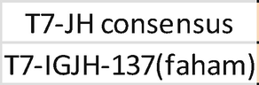
Prepare the primer mix for IGH DHJH (see Note 2).
-
3.
Prepare the primer mix for IGK (see Note 3).
-
4.
Prepare the primer mix for TRG (see Note 4).
-
5.
Prepare the primer mix for TRD (see Note 5).
-
6.
Prepare the primer mix for TRB DJ (see Note 6).
-
7.
Prepare the primer mix for TRB VDJ (see Note 7).
Importantly, each primermix should be prepared with the same index.
3.2.2 PCR Amplification
-
1.
Prepare the PCR mix for each reaction on ice (see Table 1).
-
2.
First, mix H20, buffer, and MgCl2 on ice.
-
3.
Then prepare a 0.1× dilution of Taq polymerase with H2O.
-
4.
Add primer indexes to the mix.
-
5.
Lastly, add 100 ng of patient DNA to each PCR (or 250 ng DNA for the TRG reaction).
-
6.
Run amplification protocol in a thermocycler (see Table 2).
3.3 Sample Purification
Remark: TRG samples do not need to be purified, but other targets must be purified with double purification ratio 0.6×/0.25×. Take out the AMPure XP Kit at least 30 min before use.
-
1.
Take a storage plate and add 28.8 μL of Agencourt beads per well.
-
2.
Add 48 μL of sample to the beads per well.
-
3.
Cover with an adhesive film.
-
4.
Centrifuge at 280 × g for 1 min.
-
5.
Put the plate on a microplate shaker at 200 × g for 2 min.
-
6.
Incubate the plate for 5 min at room temperature.
-
7.
Centrifuge at 280 × g for 1 min.
-
8.
Put the plate to the side skirted magnet for 5 min.
-
9.
Transfer 76 μL of supernatant to a new storage plate.
-
10.
Add to the new wells 19 μL beads for the IGH VDJ/IGK /TRD /TRB DJ/TRB VDJ reactions and 15.2 μL for the IGH-DJ reaction.
-
11.
Cover with adhesive film.
-
12.
Centrifuge at 280 × g for 1 min.
-
13.
Put the plate to the side skirted magnet for 5 min.
-
14.
Discard the supernatant and wash the beads twice with 190 μL 70% ethanol.
-
15.
Shift the plate on the side skirted magnet and wait 1 min.
-
16.
Discard all supernatant and wait 1 min.
-
17.
Leave the plate on the side skirted magnet and add 10 μL TE.
-
18.
Centrifuge at 280 × g for 1 min.
-
19.
Put the plate to the side skirted magnet for 5 min.
-
20.
Collect 8.5 μL of each sample.
3.4 Sample Assay Quantification
-
1.
Take an assay plate.
-
2.
Prepare a dilution of 199 μL ds DNA Dye buffer +1 μL purified library.
-
3.
Measure the concentration in ng/μL of samples at GLOMAX.
-
4.
Transform ng/μL into nM with this formula:
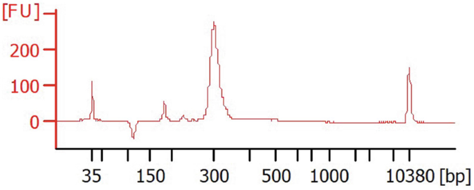
$$ =\left(\mathrm{conc}\ \mathrm{ng}/\upmu \mathrm{L}\times 10\hat{\mkern6mu} 6\right)/\left(\mathrm{size}\ \mathrm{of}\ \mathrm{library}\ \mathrm{in}\ \mathrm{base}\ \mathrm{pairs}\times 660\right). $$Option: One can verify the size of each library by electrophoresis on a Bioanalyzer 2100. Analyze 1 μL sample with the DNA High Sensitivity Agilent kit.
After migration, profiles and sizes should be as illustrated below (example is shown for TRB VDJ).
Locus
IGH R2
IGH DJ
IGK
TRG
TRD
TRB DJ
TRB VDJ
Median size (pb)
430
250
300
260
300
300
300

3.5 Pool Preparation (2 nM)
-
1.
Make a dilution at 2 nM of each sample with TE.
-
2.
Make an equimolar pool at 2 nM with 5 μL of each sample.
-
3.
Measure the concentration of the pool by Qubit.
-
4.
Transform ng/μL into nM with this formula:
$$ =\left(\mathrm{conc}\ \mathrm{ng}/\upmu \mathrm{L}\times 10\hat{\mkern6mu} 6\right)/\left(\mathrm{size}\ \mathrm{of}\ \mathrm{library}\ \mathrm{in}\ \mathrm{base}\ \mathrm{pair}\times 660\right). $$
3.6 Denaturation Step
-
1.
Normalize the library pool to 2 nM in Resuspension Buffer.
-
2.
Prepare 0.1 N NaOH: 5 μL 2 N NaOH +95 μL H2O (or 1 μL 10 N NaOH +99 μL H2O).
-
3.
Vortex.
-
4.
Put the HT1 tube in ice.
-
5.
Add in an Eppendorf tube: 5 μL library pool 2 nM + 5 μL 0.1 N NaOH.
-
6.
Vortex.
-
7.
Centrifuge quickly.
-
8.
Incubate for 5 min at room temperature (DNA denaturation).
-
9.
Add 823 μL ice-cold HT1 to prepare a 12 pM denatured library pool.
-
10.
Vortex.
-
11.
Centrifuge quickly.
-
12.
Place the Eppendorf tube on ice until it settles in the cartridge.
-
13.
Add in another Eppendorf tube 120 μL 20 pM denatured PhiX library +80 μL ice-cold HT1 to prepare a 12pM denatured PhiX library.
-
14.
Vortex.
-
15.
Centrifuge quickly.
-
16.
Place the Eppendorf tube on ice.
Adding 10% of PHIX control in pool library:
-
(a)
In 2 mL low bind tube: 540 μL 12pM denatured library pool +60 μL 12pM denatured PhiX library.
-
(b)
Vortex.
-
(c)
Centrifuge quickly.
-
(d)
Place the Eppendorf tube in ice.
-
(e)
Load 600 μL into the “load sample” well of the MiSeq cartridge V2.
3.7 Bioinformatic Analysis with the Vidjil Platform
-
1.
Copy each of the FASTQ files in the folder MiSeq Output.
-
2.
Connect to the Vidjil server [11] with a personal login and password.
-
3.
Create a “run” and as many “patients” as necessary (see Fig. 1).
-
(a)
Click on runs and then on new runs.
-
(b)
Fill information on the run (date, metadata on the sample using tags prefixed with a #). Afterwards, the samples can be searched by tags.
-
(c)
Add as many patients as required and specify a first and last name for each case.
-
(a)
-
4.
Open the created run and click on the Add samples button.
-
(a)
Select the pre-process M + R2: Merge paired-end reads (A in Fig. 2).
-
(b)
Click on Add other sample to have as many sample lines as required (B in Fig. 2).
-
(c)
Add each sample one by one.
-
Select the FASTQ file for the R1 reads in the first field (C in Fig. 2).
-
Select the FASTQ file for the R2 reads in the second field (D in Fig. 2).
-
Enter the sampling date.
-
In the last field, type the last name of the patient and select the corresponding one in the list that appears (E in Fig. 2). This will associate the sample to the patient, which will then be available from run or patient.
-
-
(a)
-
5.
Submit the samples.
-
6.
Choose the configuration of the algorithm: “multi+inc+xxx.” This is the advised configuration for target identification as it will detect both complete and incomplete recombinations (Fig. 3).
-
7.
Launch the analysis with the selected configuration for each sample.
-
8.
Click on reload, at the bottom left, to see the job status going through the different steps: QUEUED → ASSIGNED → RUNNING → COMPLETED. It is possible to launch several processes at the same time (some will wait in the QUEUED/ASSIGNED states).
-
9.
Once the jobs are completed, return to the patient list to visualize the results by clicking on the configuration name.
-
10.
Analyze the sample to determine the markers of interest (Fig. 4).
-
(a)
The percentage of analyzed reads should normally be above 90%; otherwise the sequencing run may be of poor quality (A in Fig. 4).
-
In case this percentage is too low, investigate the reason why by clicking on the info button in the upper left panel (B in Fig. 4).
-
Specifically, check the percentage of reads that are classified as:
-
UNSEG only V/5′ (reads only matching V genes).
-
UNSEG only J/3′ (reads only matching J genes).
-
UNSEG too few V/J (reads matching no V or J gene).
-
-
-
(b)
Identify the loci of interest, with at least 10,000 reads (C in Fig. 4).
-
(a)
-
11.
Study each clonotype of interest one by one.
-
12.
Switch in order to each of those loci.
-
13.
Cluster all sub-clonotypes linked to the clonotype being studied.
-
(a)
Select all the clonotypes with the same V and J genes as the studied clonotype .
-
(b)
Align the sequences (D in Fig. 4).
-
(c)
Remove the sequences that do not align properly with the studied clonotype .
-
(d)
Realign the sequences.
-
(e)
Restart steps c and d until all the sequences align with only few differences.
-
(f)
Cluster the aligned sequences (button cluster, E in Fig. 4).
-
(a)
-
14.
Send the clonotypes to IMGT/V-QUEST [12,13,14,15], by clicking on the IMGT button (F in Fig. 4). Next the V, D, and J genes as computed by IMGT/V-QUEST are underlined. This must be taken into account for the design of the patient-specific primer in case of MRD analysis by qPCR.
-
15.
Save the analysis by going to the menu at the top left corner and click on save.

Adding patients and runs in Vidjil

Adding samples in Vidjil. The rectangles refer to the different steps described in the main text

Selecting configuration and launching Vidjil-algo processes

Analyzing the clonotypes in the Vidjil client. Clonotypes are viewed at the same time in a Genescan-like view, a grid view (depending on V/J genes) and in a list. Moreover, the sequences of the selected clonotypes appear at the bottom
4 Notes
-
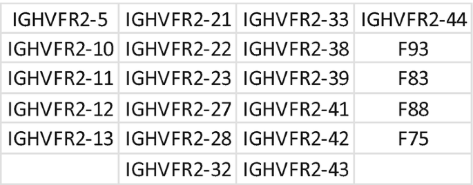
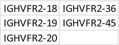
1.
Primer mix for IGH VDJ FR2. Each primer should be mixed with the same index; mixing of primers needs to be repeated for each unique index. Prepare a 1.5 mL low bind tube for primer mixes A, B, and C:
-
(a)
Tube A: combine primer for index D502.
-
Add 2 μL of each primer at 100 μM + 396 μL H2O; each primer is at 10 μM.
-
-
(b)
Tube B: combine primer for index D502.
-
Add 2 μL of each primer at 100 μM + 90 μL H2O; each primer is at 10 μM.
-
-
(c)
Tube C: combine primer for index D701.
-
Add 2 μL of each primer at 100 μM + 36 μL H2O; each primer is at 10 μM.

-
-
(a)
-
2.
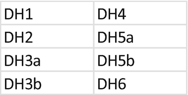
Primer mix for IGH DHJH. Each primer should be mixed with the same index; mixing of primers needs to be repeated for each unique index. Prepare a 1.5 mL low bind tube for primer mixes of DH primers and JH primers:
-
(a)
Tube DH primer: combine primer for index D502.
-
Add 2 μL of each primer at 10 μM; each primer is at 10 μM.
-
-
(b)
Tube JH primer: combine primer for index D701.
-
Add 2 μL of each primer at 100 μM + 36 μL H2O; each primer is at 10 μM.
-
-
(a)
-
3.
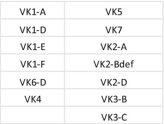
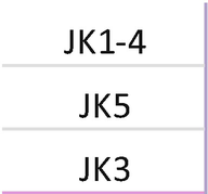
Primer mix for IGK . Each primer should be mixed with the same index; mixing of primers needs to be repeated for each unique index. Prepare a 1.5 mL low bind tube for primer mix Vkappa, Intron, Jkappa, and Kde:
-
(a)
Tube Vkappa: combine primer for index D502.
-
Add 5 μL of each primer at 100 μM + 585 μL H2O; each primer is at 10 μM.
-
-
(b)
Tube Intron: primer for index D502.
-
Dilute 5 μL of each primer at 100 μM + 45 μL H2O.
-
-
(c)
Tube Jkappa: combine primer for index D701.
-
Add 4 μL of each primer at 100 μM + 108 μL H2O; each primer is at 10 μM.
-
-
(d)
Tube Kde: primer for index D701.
-
Dilute 5 μL of each primer at 100 μM + 45 μL H2O.
-
-
(a)
-
4.
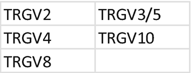
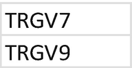
Primer mix for TRG . Each primer should be mixed with the same index; mixing of primers needs to be repeated for each unique index. Prepare a 1.5 mL low bind tube for primer mix A TCRGV, mix B TCRGV, and mix C TCRGJ, TCRGV11:
-
(a)
Tube mix A TCRGV: combine primer for index D502.
-
Add 2 μL of each primer at 100 μM + 90 μL H2O; each primer is at 10 μM.
-
-
(b)
Tube mix B TCRGV: combine primer for index D502.
-
Add 2 μL of each primer at 100 μM + 36 μL H2O; each primer is at 10 μM.
-
-
(c)
Tube TCRGV11: primer for index D502.
-
Dilute 1 μL of each primer at 100 μM + 36 μL H2O.
-
-
(d)
Tube mix C TCRGJ: primer for index D701.
-
Mix 7 μL of each primer at 20 μM.

-
-
(a)
-
5.
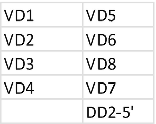
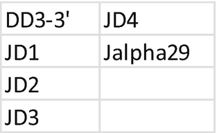
Primer Mix for TRD . Each primer should be mixed with the same index; mixing of primers needs to be repeated for each unique index. Prepare a 1.5 mL low bind tube for primer mix VDD2 and mix JDD:
-
(a)
Tube mix VDD2: combine primer for index D502.
-
Mix 5 μL of each primer at 100 μM.
-
-
(b)
Tube mix JDD: combine primer for index D701.
-
Mix 5 μL of each primer at 100 μM.
-
-
(a)
-
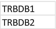
6.
Primer mix for TRB DJ. Each primer should be mixed with the same index; mixing of primers needs to be repeated for each unique index. Prepare a 1.5 mL low bind tube for primer mix TRB DB and mix TRB JB:
-
(a)
Tube mix TRB DB: combine primer for index D502.
-
Mix 2 μL of each primer at 10 μM + 36 μL H2O.
-
-
(b)
Tube mix TRB JB: combine primer for index D701.
-
Mix 2 μL of each primer at 10 μM + 252 μL H2O.
-
-
(a)
-
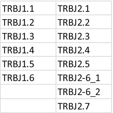
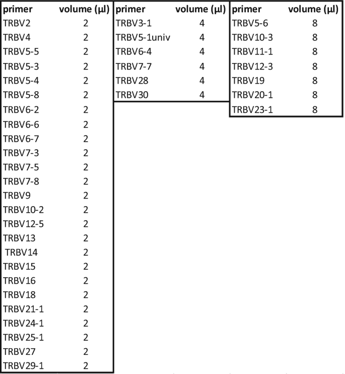
7.
Primer mix for TRB VDJ. Each primer should be mixed with the same index; mixing of primers needs to be repeated for each unique index. Prepare a 1.5 mL low bind tube for primer mix TRB VB and mix TRB JB:
-
(a)
Tube mix TRB VB: combine primer for index D502.
-
Mix each primer at 100 μM with the volume below:
-
-
(b)
Tube mix TRB JB: combine primer for index D701.
-
Mix 2 μL of each primer at 10 μM + 252 μL H2O.

-
-
(a)


References
Tonegawa S (1983) Somatic generation of antibody diversity. Nature 302(5909):575–581
Evans PAS, Pott C, Groenen PJTA, Salles G, Davi F, Berger F et al (2007) Significantly improved PCR-based clonality testing in B-cell malignancies by use of multiple immunoglobulin gene targets. Report of the BIOMED-2 concerted action BHM4-CT98-3936. Leukemia 21(2):207–214
Langerak AW, Groenen PJTA, Brüggemann M, Beldjord K, Bellan C, Bonello L et al (2012) EuroClonality/BIOMED-2 guidelines for interpretation and reporting of Ig/TCR clonality testing in suspected lymphoproliferations. Leukemia 26(10):2159–2171
van Dongen JJM, Langerak AW, Brüggemann M, Evans PA, Hummel M, Lavender FL et al (2003) Design and standardization of PCR primers and protocols for detection of clonal immunoglobulin and T-cell receptor gene recombinations in suspect lymphoproliferations: report of the BIOMED-2 concerted action BMH4-CT98-3936. Leukemia 17(12):2257–2317
Langerak AW, Brüggemann M, Davi F, Darzentas N, van Dongen JJM, Gonzalez D et al (2017) High-throughput Immunogenetics for clinical and research applications in immunohematology: potential and challenges. J Immunol 198(10):3765–3774
Scheijen B, Meijers RWJ, Rijntjes J, van der Klift MY, Möbs M, Steinhilber J et al (2019) Next-generation sequencing of immunoglobulin gene rearrangements for clonality assessment: a technical feasibility study by EuroClonality-NGS. Leukemia 33(9):2227–2240
Kotrova M, Trka J, Kneba M, Brüggemann M (2017) Is next-generation sequencing the way to go for residual disease monitoring in acute lymphoblastic leukemia? Mol Diagn Ther 21(5):481–492
Logan AC, Gao H, Wang C, Sahaf B, Jones CD, Marshall EL et al (2011) High-throughput VDJ sequencing for quantification of minimal residual disease in chronic lymphocytic leukemia and immune reconstitution assessment. Proc Natl Acad Sci U S A 108(52):21194–21199
Wu D, Sherwood A, Fromm JR, Winter SS, Dunsmore KP, Loh ML et al (2012) High-throughput sequencing detects minimal residual disease in acute T lymphoblastic leukemia. Sci Transl Med 4(134):134ra63
Brüggemann M, Kotrová M, Knecht H, Bartram J, Boudjogrha M, Bystry V et al (2019) Standardized next-generation sequencing of immunoglobulin and T-cell receptor gene recombinations for MRD marker identification in acute lymphoblastic leukaemia; a EuroClonality-NGS validation study. Leukemia 33(9):2241–2253
Giraud M, Salson M, Duez M, Villenet C, Quief S, Caillault A et al (2014) Fast multiclonal clusterization of V(D)J recombinations from high-throughput sequencing. BMC Genomics 15:409
Alamyar E, Duroux P, Lefranc M-P, Giudicelli V (2012) IMGT(®) tools for the nucleotide analysis of immunoglobulin (IG) and T cell receptor (TR) V-(D)-J repertoires, polymorphisms, and IG mutations: IMGT/V-QUEST and IMGT/HighV-QUEST for NGS. Methods Mol Biol 882:569–604
Aouinti S, Giudicelli V, Duroux P, Malouche D, Kossida S, Lefranc MP (2016) IMGT/StatClonotype for pairwise evaluation and visualization of NGS IG and TR IMGT clonotype (AA) diversity or expression from IMGT/HighV-QUEST. Front Immunol 7:339
Lefranc M-P (2014) Immunoglobulin and T cell receptor genes: IMGT® and the birth and rise of Immunoinformatics. Front Immunol 5:22
Lefranc M-P, Giudicelli V, Duroux P, Jabado-Michaloud J, Folch G, Aouinti S et al (2015) IMGT®, the international ImMunoGeneTics information system® 25 years on. Nucleic Acids Res 43(Database issue):D413–D422
Author information
Authors and Affiliations
Corresponding author
Editor information
Editors and Affiliations
Rights and permissions
Open Access This chapter is licensed under the terms of the Creative Commons Attribution 4.0 International License (http://creativecommons.org/licenses/by/4.0/), which permits use, sharing, adaptation, distribution and reproduction in any medium or format, as long as you give appropriate credit to the original author(s) and the source, provide a link to the Creative Commons license and indicate if changes were made.
The images or other third party material in this chapter are included in the chapter's Creative Commons license, unless indicated otherwise in a credit line to the material. If material is not included in the chapter's Creative Commons license and your intended use is not permitted by statutory regulation or exceeds the permitted use, you will need to obtain permission directly from the copyright holder.
Copyright information
© 2022 The Author(s)
About this protocol

Cite this protocol
Villarese, P. et al. (2022). One-Step Next-Generation Sequencing of Immunoglobulin and T-Cell Receptor Gene Recombinations for MRD Marker Identification in Acute Lymphoblastic Leukemia. In: Langerak, A.W. (eds) Immunogenetics. Methods in Molecular Biology, vol 2453. Humana, New York, NY. https://doi.org/10.1007/978-1-0716-2115-8_3
Download citation
DOI: https://doi.org/10.1007/978-1-0716-2115-8_3
Published:
Publisher Name: Humana, New York, NY
Print ISBN: 978-1-0716-2114-1
Online ISBN: 978-1-0716-2115-8
eBook Packages: Springer Protocols