
Abstract
The standard model (e.g., Hocking in Earth Planets Space 51:525–541, 1999), \(\varepsilon = c_{0} \sigma^{2} N\), (where \(\sigma\) is the radar spectral width assumed to be equal to vertical turbulence velocity fluctuation \(\sqrt {\overline{{w^{2} }} }\), N is the buoyancy frequency, and c0 is a constant), derived from Weinstock (J Atmos Sci 35:1022–1027, 1978; J Atmos Sci 38:880–883, 1981) formulation, has been used extensively for estimating the turbulence kinetic energy (TKE) dissipation rate \(\varepsilon\) under stable stratification from VHF radar Doppler spectral width \(\sigma\). The Weinstock model can be derived by simply integrating the TKE spectrum in the wavenumber space from the buoyancy wavenumber \(k_{\text{B}} = \frac{N}{\sigma }\) to \(\infty\). However, it ignores the radar volume dimensions and hence its spatial weighting characteristics. Labitt (Some basic relations concerning the radar measurements of air turbulence, MIT Lincoln Laboratory, ATC Working Paper NO 46WP-5001, 1979) and White et al. (J Atmos Ocean Technol 16:1967–1972, 1999) formulations do take into account the radar spatial weighting characteristics, but assume that the wavenumber range in the integration of TKE spectrum extends from 0 to \(\infty\). The White et al. model accounts for wind speed effects, whereas the other two do not. More importantly, all three formulations make the assumption that k−5/3 spectral shape of TKE spectrum extends across the entire wavenumber range of integration. It is traditional to use Weinstock formulation for \(k_{\text{B}}^{ - 1} < 2a,2b\) (where a and b are radar volume dimensions in the horizontal and vertical directions) and White et al. formulation (without wind advection) for \(k_{\text{B}}^{ - 1} > 2a,2b\). However, there is no need to invoke these asymptotic limits. We present here a numerical model, which is valid for all values of buoyancy wavenumber \(k_{\text{B}}\) and transitions from \(\varepsilon \sim\sigma^{2}\) behavior at lower values of \(\sigma\) in accordance with Weinstock’s model, to \(\varepsilon \sim\sigma^{3}\) at higher values of \(\sigma\), in agreement with Chen (J Atmos Sci 31:2222–2225, 1974) and Bertin et al. (Radio Sci 32:791–804, 1997). It can also account for the effects of wind speed, as well the beam width and altitude. Following Hocking (J Atmos Terr Phys 48:655–670, 1986, Earth Planets Space 51:525–541, 1999), the model also takes into account contributions of velocity fluctuations beyond the inertial subrange. The model has universal applicability and can also be applied to convective turbulence in the atmospheric column. It can also be used to explore the parameter space and hence the influence of various parameters and assumptions on the extracted \(\varepsilon\) values. In this note, we demonstrate the utility of the numerical model and make available a MATLAB code of the model for potential use by the radar community. The model results are also compared against in situ turbulence measurements using an unmanned aerial vehicle (UAV) flown in the vicinity of the MU radar in Shigaraki, Japan, during the ShUREX 2016 campaign.

Introduction
The dissipation rate \(\varepsilon\) of turbulence kinetic energy (TKE) is a fundamental parameter indicative of the strength of turbulence. With suitable assumptions, knowledge of \(\varepsilon\) allows the turbulent diffusion coefficient K, of great importance to mixing in the fluid column, to be determined. As such there is considerable interest in determining \(\varepsilon\) in both the atmosphere and the oceans. While the principal application of VHF wind profiling Doppler radars is for measuring the three components of wind velocity in the atmospheric column, they also have the capability to measure velocity fluctuations in the beam direction. The intensity of velocity fluctuations can be determined from the spectral width \(\sigma\) of the backscattered signal, after suitable corrections are applied to effects such as beam broadening and wind shear. The task then is to infer the dissipation rate from the spectral width. But first, the dissipation rate has to be related to turbulent velocity fluctuations. Considerable effort has been expended over the past four decades on the problem of extracting \(\varepsilon\) from \(\sigma\). A very useful summary of these efforts and the issues involved can be found in an excellent review by Hocking (1999).
Simultaneous measurements of \(\varepsilon\) by the radar and in situ turbulence sensors, both measuring the same volume, have been costly and hence infrequent (but see Bertin et al. 1997; Dehghan and Hocking 2011; Dehghan et al. 2014 and the references cited therein). As such, there are still some unresolved issues. However, quite recently, routine and inexpensive in situ measurements have been made possible through turbulence sensors deployed on small, unmanned aerial vehicles (UAVs, e.g., Scipion et al. 2016) flown near and above the MU radar in Shigaraki, Japan (Kantha et al. 2017; Luce et al. 2018). This has enabled us to revisit the problem of extracting \(\varepsilon\) from \(\sigma\). A brief summary of past work is also provided for completeness and context.
Weinstock (1978, 1981) was one of the first to propose a model that enables extraction of \(\varepsilon\) from measurements of vertical turbulence velocity fluctuations \(\overline{{w^{2} }} = \sigma_{w}^{2}\) and the local buoyancy frequency N:
where c0 is an empirical constant and N, the buoyancy frequency indicative of the degree of stability of the fluid column, is given by:
where g is the gravitational acceleration, z is the vertical coordinate, and \(\varTheta\) is the potential temperature (assuming dry air, although water vapor effects can be easily incorporated through virtual potential temperature).
The Weinstock model was subsequently applied to Doppler MST radars operating in the VHF-band (e.g., Hocking 1983, 1985, 1986, 1999; Fukao et al. 1994) to extract \(\varepsilon\) from measurements of turbulence-produced radar spectral width \(\sigma\), with the assumption
so that
The extraction of the Doppler variance due to turbulence after correcting for beam-broadening and shear-broadening effects is outside the scope of the present work. Here, we assume that \(\sigma\) is correctly evaluated but can be affected by wave contributions. Equation (4) has been used extensively since, for estimating the turbulence kinetic energy (TKE) dissipation rates under stable stratification from VHF radar Doppler spectra, although there is still considerable debate as to the exact value of c0. In a nice summary, Hocking et al. (2016) show that its empirical value appears to vary between 0.27 and 0.6, but recommend that \(0.5 \pm 0.25\) be used (their Eq. 7.55). However, as shown below, c0 depends on the Kolmogorov universal constant \(\alpha\) as well as the lower limit of integration of the turbulence wavenumber spectrum.
The primary dependence of \(\varepsilon\) is on \(\sigma_{w}\) (or equivalently \(\sigma\) when applied to radar data), since the dependence on N is much weaker. As such, Weinstock model yields \(\varepsilon \sim \sigma_{w}^{2}\) (or equivalently \(\sigma^{2}\)) behavior, whereas \(\varepsilon \sim\sigma_{w}^{3}\) (or equivalently \(\sigma^{3}\)) dependence based on some stratospheric measurements of turbulence is also evident in some cases (Chen 1974; Bertin et al. 1997). The latter behavior suggests \(\varepsilon \sim \frac{{\sigma^{3} }}{L}\), where L is a turbulence length scale (independent of N). It is possible that under certain conditions (Hocking 1999), L could remain constant giving rise to \(\varepsilon \sim\sigma^{3}\) behavior. Labitt (1979) proposed a model that yields \(\varepsilon \sim\sigma^{3}\) behavior.
But first, it is useful to define the various wavenumbers (and length scales) involved in the above models and derivations, since there appears to be some confusion about exact definitions that complicate the debate (see Section 3 of Hocking 1999) and introduce uncertainties into the estimation of some constants. The Kolmogorov viscous wavenumber of importance in turbulence studies defined as
corresponds to the Kolmogorov viscous scale, indicative of the scales at which dissipation of TKE cascading down the spectrum from large energy-containing scales to viscous dissipative scales, takes place. (\(\nu\) is the kinematic viscosity.) This Kolmogorov viscous scale is traditionally defined (without the factor \(2\pi\)) as:
If the turbulence Reynolds number is large enough, sufficiently far away from anisotropic energy-containing wavenumbers (equivalently scales), the turbulence kinetic energy spectrum contains the Kolmogorov universal range, where the spectral shape depends only on the wavenumber k, the TKE dissipation rate \(\varepsilon\) and the Kolmogorov viscous scale \(\eta\):
where the proportionality constant \(\alpha\) is known as the Kolmogorov universal constant and f stands for function. One frequently used form for the spectrum in the universal range (e.g., Ogura 1958) is
where \(\kappa = 0.4\) is the von-Karman constant. Turbulent eddies are expected to be isotropic in the Kolmogorov universal range of the energy spectrum, the idea being that while the large energy-containing scales are necessarily anisotropic (especially under the influence of buoyancy or other directional forces), as the energy cascades down the spectrum to higher wavenumbers by nonlinear interactions, the turbulent eddies lose memory of directionality and become increasingly isotropic.
For \(k\eta > > 1,\) viscous subrange (VSR) results and the spectrum take the form:
where \(\beta \sim0.041\).
Far away from both isotropic viscous and anisotropic energy-containing scales, if the turbulence Reynolds number is high enough, lies the inertial subrange (ISR) of the Kolmogorov universal spectrum, whose shape depends only on the wavenumber k and the dissipation rate \(\varepsilon\), and not on the Kolmogorov viscous scale \(\eta\):
There has been an enormous amount of work done over the years to determine the precise value of \(\alpha\) and as a result, it is known to range between 1.53 and 1.65 (e.g., Gossard et al. 1984). The best-known empirical value at present is 1.65 (although 1.53 has also been used, e.g., Weinstock 1981; Hocking 1999). This value is very close to the often-cited (e.g., Ogura 1958) value of \(\left( {\frac{8}{9\kappa }} \right)^{2/3} \sim1.675\). Note that the Kolmogorov universal range consists of the inertial and viscous subranges and the transition between the two.
It is also important to keep in mind the fact that when the upper limit on the wavenumber in the integration of energy spectrum is taken as infinity, strictly speaking, Eq. (8) should be used instead of Eq. (10).
Empirically, the inner scale of turbulence corresponding to the inner edge of the ISR is taken to correspond to the upper wavenumber limit of the ISR and is related to the Kolmogorov viscous wavenumber (e.g., Wilson 2004):
where kK is the Kolmogorov wavenumber (Eq. 5). Note that the proportionality constant in Eq. (11) is not far from the value \(4\pi\). The inner scale is therefore
In stably stratified flows, buoyancy forces tend to flatten large turbulent eddies and make them anisotropic, so that vertical velocity fluctuations become less than the horizontal ones, the degree of reduction depending on the stability of the fluid column. The lower wavenumber limit of the ISR is therefore determined by the Ozmidov wavenumber
The wavenumber corresponding to the outer scale of turbulence denoting the outer edge of the ISR is proportional to the Ozmidov wavenumber so that the outer scale is
where \(f_{k} = \frac{{k_{\text{OUT}} }}{{k_{\text{O}} }}\) is the ratio of the outer and Ozmidov wavenumbers. While theoretical studies such as Sukorianski and Galperin (2017) assert that the transition between the inertial and buoyancy subranges lies close to the Ozmidov scale 1/kO, thus suggesting the value of this ratio is close to 1.0, its precise value remains uncertain at present and should perhaps be determined by dedicated experiments in the future (personal communication by W. Hocking). The code allows for the user to prescribe the value of the proportionality constant fK.
The outer and inner scales of turbulence denote the edges of the ISR. The ratio of the two is
where
is the so-called buoyancy Reynolds number, used routinely by oceanographers as a measure of “turbulence activity,” indicative of the “strength” of turbulence as measured by microstructure profilers in the ocean (e.g., Gregg et al. 2018). The ratio R itself is indicative of the extent of the ISR in the turbulence energy spectrum. Assuming fk = 1, for Reb ~ 645, the ISR extends over a decade of wavenumbers (R = 10) and for Reb ~ 13,900, over 2 decades (R = 100). In the stably stratified regions of both the oceans and the atmosphere, the value of R lies mostly but not entirely between 10 and 100.
At wavenumbers less than the Ozmidov wavenumber kO (or equivalently scales larger than the Ozmidov length scale LO), buoyancy forces begin to affect turbulence by tending to inhibit vertical motions. The turbulence spectral shape may deviate from that in the ISR. This buoyancy subrange (BSR) is thought to extend from the outer wavenumber kOUT to the buoyancy wavenumber kB defined as
The length scales corresponding to the Ozmidov and buoyancy wavenumbers are known as Ozmidov and buoyancy length scales and can be defined as the reciprocal of kO and kB, respectively (without the factor \(2\pi\))
This is the definition that atmospheric scientists use (e.g., American Meteorological Society), although some studies (e.g., Weinstock 1981; Hocking 1999) define the buoyancy scale as \(2\pi /k_{\text{B}}\). The Ozmidov length scale is also often defined as \(2\pi /k_{\text{O}}\). There has been considerable and needless confusion regarding length scales we use in turbulence studies (see also comments in Section 3 of the review of the topic by Hocking 1999) because of the factor \(2\pi\), which can lead to serious discrepancies in the magnitudes of \(\varepsilon\) extracted from \(\sigma\).
However, there is a simple solution. The wavenumber spectrum is more fundamental to turbulence studies and as long as we deal with just wavenumbers, which involve no ambiguity whatsoever, and not arbitrarily defined length scales, there is no inconsistency in the derivations of the expressions for the dissipation rate (in terms of wavenumbers). Once that is done, wavenumbers can be converted to corresponding scales, whichever way they are defined. We do so and suggest that the radar community do the same, since there is usually some ambiguity as to how to define the corresponding length scales, i.e., with or without the factor \(2\pi .\) This has to do with the confusion between length scales and wavelengths in turbulence studies as we transition from the wavenumber space (see the excellent discussion in Hocking 1999, also personal communication by Hocking). Our own preference is to define turbulence length scales as inverse of wavenumbers.
The spectrum in the BSR (kOUT < k < kB), where buoyancy forces affect turbulence, is thought to follow the law
although the precise value of nb is uncertain. Weinstock (1978) suggests that the value of nb depends on the flux Richardson number, but is close to the ISR value of 5/3, while Lumley (1964; see also Sukoriansky and Galperin 2017) suggests nb = 3. In any case, the Ozmidov wavenumber kO (often called the buoyancy wavenumber in meteorology leading to needless confusion once again) is indicative of the transition from ISR to BSR in the spectrum (while buoyancy wavenumber kB is indicative of the transition from turbulent motions to wave motions), and the spectrum in the wavenumber range comprising of both ISR and BSR can be modeled as:
so that for k ≫ kOUT, the ISR results: \(E \to \alpha \varepsilon^{2/3} k^{ - 5/3}\) and for k ≪ kOUT, we get the BSR
Note that the computer code has been written so that the user can input any values for fK and nb, although in the illustrative plots, we have used fK = 1 and nb = − 5/3.
Now, fluctuations below the wavenumber kB (equivalently above the buoyancy length scale LB) are due to wave motions and not turbulence. This must be taken into account in the derivations of \(\varepsilon\), since the radar does not discriminate between velocity fluctuations due to turbulence and wave motions. Keeping in mind the fact that wave motions can exist below the buoyancy wavenumber kB, the integration of the turbulence energy spectrum E(k) over the wavenumber space kB to \(\infty\) yields the energy resident in turbulent fluctuations and only turbulent fluctuations, i.e., the TKE:
where
is twice the turbulence kinetic energy. The lower limit in Eq. (22) assures that all motions considered are due to turbulence and not from wave motions possible under stable stratification. The major portion of the contribution to TKE comes from low wavenumbers corresponding to energy-containing scales. The high wavenumbers close to viscous dissipation scales contribute very little.
Only wavenumbers (scales) smaller (larger) than the Bragg backscatter wavenumber (scale) contribute to broadening of the spectrum of the backscattered radar signal, and therefore, the upper limit of integration in Eq. (22) should be taken as
where \(\lambda\) is the wavelength of the radar, so that the TKE
It is traditional to assume that the − 5/3 shape of the spectrum representative of the ISR (shape is uncertain in the BSR) extends across the entire integration range from kB to kBragg so that using
yields
However, the radar spectral width depends only on \(\overline{{w^{2} }}\) and so further assumptions are necessary. It is usual to assume equal contributions to TKE from velocity fluctuations in the three directions (\(\overline{{u^{2} }} = \overline{{v^{2} }} = \overline{{w^{2} }}\)) so that
Then, Eq. (27) can be written as
If non-isotropy of the components of TKE is acknowledged, there would be an appropriate factor multiplying \(\alpha\) on the right hand side of Eq. (29) (see Appendix B).
Finally, for analytical convenience, it is usual to ignore the second term in the square brackets and implicitly assume kB ≪ kBragg so that
which yields:
where
as indicated by Weinstock (1978, 1981). Substituting for kB from Eq. (17) yields
which is the Weinstock (1981) model. For \(\alpha = 1.65\), c0 ~ 0.47. As such, there is no ambiguity in the value of c0, since it is tied to the Kolmogorov universal constant, if and only if the lower limit on integration is strictly enforced as equal to the buoyancy wavenumber, which delineates wave motions from turbulent motions. Application to radar spectral width data gives Eq. (4), the widely used form of Weinstock (1981) model.
The Weinstock model can also be derived as follows (e.g., Hocking 1999). Define a “buoyancy scale” as he did (recall we define the buoyancy scale differently: LB = 1/kB):
and integrate the energy spectrum from \(\frac{2\pi }{{\bar{L}_{\text{B}} }}\) to \(\infty\). But from Eq. (34),
Therefore,
Using Eq. (26), we get
which can be written as (using Eqs. 13, 28):
so that
where c0 ~ 0.44 if \(\alpha = 1.65\), but 0.47 if \(\alpha = 1.53\) as in Hocking (1999). Invoking Eq. (3), we get the Weinstock model (Eq. 4). If we had used kO as the lower limit of integration, c0 would have been 0.61.
The closeness of Eqs. (39) and (33) is merely a happenstance.
It is interesting to note that Eqs. (13) and (39) yield
for c0 = 0.47. The relative closeness of the two wavenumbers tends to downplay the influence of the exact spectral shape in the BSR portion of the spectrum.
However, the radar measurement volume is finite, and the Weinstock formulation does not take into account the resulting radar spatial weighting characteristics. On the other hand, Labitt (1979) and White et al. (1999) formulations do (see “Radar epsilon model” section), but provide numerical and not analytical solutions. However, both integrate the wavenumber spectrum of the backscattered radar signal from 0 to \(\infty\), whereas the Weinstock model integrates the turbulence spectrum from the buoyancy wavenumber kB to \(\infty\). As summarized by Hocking (1999), these three Doppler methods lead to different formulas and results, which has been a source of some confusion. Also, all three formulations make the assumption that the k−5/3 spectral shape representative of the inertial subrange (ISR) of the turbulence kinetic energy spectrum extends across the entire wavenumber integration range. This ignores the potential presence of the buoyancy subrange (BSR) within the integration range. Also, strictly speaking, the upper limit on wavenumber should be kBragg and not \(\infty\), although the difference is quite small. Finally, the observed spectral width due to velocity fluctuations in the beam direction may have contributions from wave motions and not just turbulence. We address these issues in the next section.
Radar epsilon model
The original Labitt (1979; see also Hocking 1986, 1999) formulation takes into account the radar spatial weighting function:
where a and b are radar volume dimensions in the horizontal and vertical. Because the radar beam measures velocity fluctuations transverse to the horizontal wind advecting turbulence past it, the value of CK can be less than 1 (see Appendix A of Hocking 1999), the exact value of depending on the type of turbulence (see Appendix B). However, this issue has been ignored thus far and all previous derivations in radar literature, including Labitt (1979), have assumed CK = 1. We have used CK = 0.873, appropriate to shear-generated turbulence, in this paper, keeping the transverse nature of radar measurements (for more details see Appendix B). The precise value of CK is still uncertain and requires further studies.
Note the wavenumber integration limits. Using the spectrum of vertical velocities:
where \(E(k)\) is the turbulence energy spectrum and
Integration in Eq. (41) can be carried out using Eq. (26) for E(k) appropriate to the ISR, which yields
or equivalently
where
This is what we will call the original Labitt method, which assumed k−5/3 spectral shape to exist over the entire wavenumber range of interest, from k = 0 to \(\infty\), and ignored the effect of wind advection (see Hocking 1999).
Now, Eq. (41) can be modified to take into account wind advection as indicated by Hocking (1983) and White et al. (1999). Following White et al. (1999):
assuming the wind is in the x-direction. Note that \(L = V_{\text{H}} \Delta t\), where VH is the wind speed in the horizontal direction and \(\Delta t\) is the dwell duration (duration for collecting the time series), which is 24.57 s for MU radar during the ShUREX campaigns. Using Eqs. (42)–(43) in Eq. (47), we get Eq. (2.14) of White et al. (1999):
This is what we call generalized Labitt formulation. Substituting
and expressing the integral in terms of x = kb, \(\theta\) and \(\varphi\), we get
White et al. (1999) showed that Eq. (50) can be approximated to within 2% by
Henceforth, we will not present results from White et al. formulation (Eq. 51), since they are very close to the generalized Labitt formulation (Eq. 50) and it is hard to discern any difference between the two in the plots. Note that CK = 1 in original Labitt and White et al. derivations.
Note that both White et al. (1999) and Labitt (1979) formulations integrate right through the wavenumber kB and therefore are accounting for velocity fluctuations due to wave motions below kB (albeit with spectral shape corresponding to ISR). A related minor issue with both formulations is that the upper limit should be kBragg, but this is not important since it makes little difference. On the other hand, since the lower limit is not kB, the wavenumber delineating turbulent and wave motions, integration is carried out right through kB and so the results, not surprisingly do not involve the buoyancy scale 1/kB (or equivalently the buoyancy frequency N), whereas Weinstock formulation integrates down to kB only and so its results involve N explicitly.
It is traditional to use Weinstock formulation for \(k_{\text{B}}^{ - 1} < 2a,2b\) and White et al. formulation (without wind advection and therefore L = 0) for \(k_{\text{B}}^{ - 1} > 2a,2b\), where the buoyancy length scale given by \(k_{\text{B}}^{ - 1}\) is taken to be the size of the largest eddies permitted under stable stratification (e.g., Fukao et al. 1994; Kantha and Hocking 2011; Luce et al. 2018). However, these are the two asymptotic limits. Since White et al. formulation requires numerical integration anyway, it is not any more difficult to use numerical integration of the generalized Labitt formulation, but with proper integration limits. A major advantage is that the numerical model allows for inclusion of wind advection and radar weighting characteristics, with no need for approximations whatsoever.
Since the original Labitt formulation (Eq. 46) does not account for wind advection, we use the generalized Labitt formulation (Eq. 48) instead or equivalently Eq. (50). However, we replace the spectrum used in Eq. (48), which is valid only in the ISR (Eq. 26) by one that extends from the viscous range to well beyond the ISR:
where nb = 4/3 is the spectral slope in the wave region (fK = 0.6–1, \(\gamma_{K} = 1\)). This form is used for completeness, although there is rarely any need to invoke VSR and so for all practical purposes
is quite close to Eq. (52). Thus, we get
This form has general applicability. If we put terms in the first curly bracket in Eq. (54) equal to 1 and take limits xL = 0 and \(x_{U} = \infty\), we get the generalized Labitt formulation (Eq. 50). In addition, if we put terms in the third square bracket equal to 1 (equivalently L = 0), the influence of wind advection is ignored. On the other hand, putting terms in the second curly bracket equal to 1 (equivalent to putting a, \(b = \infty\)) yields the Weinstock model, for which the lower limit must be xL = kBb. (Using xL = 0 as the lower limit makes the integral go to \(\infty\) thus giving \(\varepsilon = 0\).)
The numerical model presented in this paper integrates Eq. (54) in 3 segments: 1) universal range (VSR and ISR) (k = kO to k = kBragg), 2) BSR (k = kB to k = kO) and 3) Beyond BSR when wave contributions are included (k = 0 to k = kB), so that xL = 0 and xU = kBraggb. However, the principal problem is that the Ozmidov wavenumber kO is not known a priori, since it depends on the yet to be determined \(\varepsilon\). So an iterative procedure is necessary, using an initial guess value for \(\varepsilon\) from one of the standard formulations (e.g., White et al. 1999).
We illustrate the various model results in Fig. 1. The numerical model simulation is specifically for the 46.5 MHz MU radar in Shigaraki, Japan, with b = 75 m, and \(\lambda = 6.4516\) m (but can be done for any radar). The two-way half-power beam half-width is 1.32°, which determines the parameter a as a function of altitude above ground level (AGL). For the results in Fig. 1, the altitude has been set to 2 km, the average altitude of UAV measurements. The buoyancy frequency N is kept fixed at 0.0121 s−1, a value appropriate to the troposphere. The wind speed VH is put to zero, for simplicity.

Plot of the TKE dissipation rate \(\varepsilon\) against \(\sigma\) (left) and the corresponding buoyancy length scale 1/kB (right). The blue line shows the numerical model (Eq. 54). The red line shows the Weinstock (1978, 1981) formulation, while the black line is the Labitt formulation. Note that because the constant CK < 1, the numerical model does not asymptote to Weinstock and Labitt values
The left panel shows \(\varepsilon\) plotted against \(\sigma\), while the right panel shows \(\varepsilon\) plotted against the buoyancy scale 1/kB (The two plots have equivalent information.) The red line shows the Weinstock formulation (Eq. 1 with N = 0.0121 s−1), and the black line shows the general Labitt formulation denoted as G Labitt. Note that because wind = 0, the general Labitt formulation reduces to the original Labitt formulation. These two form the two asymptotic limits discussed earlier and the numerical model (blue line) transitions from one to the other quite nicely. The blue line parallels the red line for low values of \(\sigma\) and therefore 1/kB, but transitions toward the red line at high values of \(\sigma\) and 1/kB. This is simply because when 1/kB < 2a, 2b, the dissipation rate \(\varepsilon \sim\sigma^{2}\) (Weinstock 1981, but with N ~ constant), but transitions to \(\varepsilon \sim\sigma^{3}\) behavior when 1/kB > 2a, 2b (Chen 1974). Therefore, when the radar volume spatial characteristics are taken into account, both behaviors become feasible. Note that the value of CK has been put equal to 0.873. This is the reason the numerical model values do not asymptote to Weinstock and Labitt values. They would have if CK were to have been chosen equal to 1.0 (see Appendix B for details).
Figure 2 compares the numerical model results (blue line) to in situ measurements of \(\varepsilon\) made using UAV-borne turbulence sensors for all 16 flights during the ShUREX (Shigaraki UAV Radar Experiment) 2016 campaign, as detailed in Luce et al. (2018) and explained in Kantha et al. (2017). Only radar data from the vertical beam are considered. Radar data with values of \(\sigma < 0.1\) m/s (the radar noise threshold, equivalently LB < 8 m) and UAV data with \(\varepsilon < 1.1\) × 10−5 m3 s−2 (UAV sensor noise threshold) are omitted. The models mentioned in Fig. 1 are also shown. The magenta line is given by
where L = 25 m, and is in better agreement with UAV data than both the Weinstock and Labitt models. Luce et al. (2018) also suggest that Eq. (55) with L = 25 m, best fits the ShuREX 2016 UAV data. The Labitt (1979) formulation (and White et al. 1999) yields \(\varepsilon \sim\sigma^{3}\) behavior for ALL values of \(\sigma\), simply because the lower limit on integration in these formulations is zero and not kB. Note that, like in Fig. 1, because wind = 0, the general Labitt formulation reduces to the original Labitt formulation.

Plot of the TKE dissipation rate \(\varepsilon\) against \(\sigma\) (left) and the corresponding buoyancy length scale 1/kB (right). Cyan circles show the UAV-measured \(\varepsilon\) plotted against radar-determined \(\sigma\) for all 16 flights made during the ShUREX 2016 campaign. The blue line shows the numerical model (Eq. 54). The red line shows the Weinstock (1978, 1981) formulation, while the black line is the Labitt formulation. The magenta line corresponds to Eq. (55) with L = 25 m (see text). The green and magenta lines nearly overlap. Chen (1974) and other data cited in Fig. 2 of Weinstock (1981) are shown by filled red polygons. The units and the figure aspect ratio are selected to be similar to that in Figure 2 of Weinstock (1981) for easy comparison
The upper wavenumber limit has some impact. If kBragg and not \(\infty\) is imposed as the upper limit, the blue line (model), instead of overlapping the red line (Weinstock) at low values of \(\sigma\), would deviate increasingly from it as \(\sigma\) decreases, with \(\varepsilon\) values somewhat higher (not shown) than those given by Weinstock formulation.
Now, the dissipation rate in turbulent flows can be written as
where \(\ell\) is the turbulence length scale, a measure of the size of energy-containing large eddies and hence proportional to it. B1 ~ 16.6 (Kantha and Carniel 2009). For stably stratified conditions, \(\frac{{\overline{{w^{2} }} }}{{q^{2} }}\) becomes a function of the gradient Richardson number \(Ri = \frac{{N^{2} }}{{S^{2} }}\) (S is the mean shear) (e.g., Kantha and Carniel 2009). Observational data suggest that \(\frac{{\overline{{w^{2} }} }}{{q^{2} }}\) ~ 0.13–0.15 in the Ri range 0–0.25 of interest in stably stratified flows (Kantha and Carniel 2009, their Fig. 5). Taking an average value of 0.14, Eq. (56) becomes
Equating (55) and (57), it is seen that \(L = 0.4\ell\), and therefore, the turbulence length scale is around 60 m, on the average, in ShUREX 2016 measurements.
The advantage of the numerical model is that it can account for the effects of altitude and beam angle, the influence of wind advection, as well as allow imposing the upper wavenumber limit of kBragg. Figure 3 shows the effect of wind speed and altitude at the MU radar site. The acquisition time DT is ~ 30 s. Weinstock (red line) and original Labitt model (black line) for AGL (above ground level) altitude 2 km and zero wind speed are also shown for comparison. Results for 4 cases are shown. The blue line is the model result for AGL altitude of 2 km and zero wind speed, the same as the blue line in Fig. 1. The magenta line is for AGL altitude of 10 km and zero wind speed. The cyan line is for AGL altitude of 2 km and 10 m/s wind speed. The green line for AGL altitude of 10 km and wind speed of 10 m/s is nearly indistinguishable from and hence overwrites the cyan and magenta lines. It is interesting to note that all these values fall above the Weinstock values. These simulations therefore demonstrate the importance of not only imposing proper integration limits, but also accounting for the altitude AGL and wind speed for a particular radar, when deriving \(\varepsilon\) from \(\sigma\). The use of the two asymptotic limits (Weinstock and White et al.) is therefore not always justified.

Plot of the TKE dissipation rate \(\varepsilon\) against \(\sigma\) (left) and the buoyancy length scale LB (right) for various wind speeds and AGL altitudes. The black line is for White et al. (1999) formulation for zero wind speed and 2 km altitude. The red line is the Weinstock formulation. The numerical model results are: blue line for altitude = 2 km, wind speed = 0 m/s, cyan line for altitude = 2 km, wind speed = 10 m/s, magenta line for altitude = 10 km, wind speed = 0 m/s, and green line for altitude = 10 km, wind speed = 10 m/s. Note that the cyan and magenta lines have essentially been overwritten by the green line
We have provided model results only for the MU radar, since that was where in situ UAV measurements were made. It is also not possible to explore here the large parameter space that governs the \(\varepsilon\) estimates of the numerical model. Instead, the Appendix provides a MATLAB code suited to exploring the parameter space for any radar.
Correcting radar spectral width for wave contributions
Figures 1, 2, 3 assume that the spectral radar width \(\sigma\) results from velocity fluctuations due to turbulent motions only. In reality, wave motions also cause velocity fluctuations in the beam direction that contribute to \(\sigma\). For comparisons with measurements of \(\varepsilon\) by in situ turbulence sensors, it may be necessary to correct for wave motions (see Hocking 1988). This can be done as follows. If we recall
contains contributions from turbulent motions only, whereas
contains contributions from wave motions as well (because of the lower limit of integration), using Eq. (44),
is the required correction of radar measured spectral width for wave motions.
Extension to convective mixing
While we focused on turbulence in stably stratified flows so far, the general Labitt formulation can also be extended to convective mixing of any type seen in the atmospheric column, by recognizing that in this case, the ISR extends over the entire wavenumber range of interest. Neither the Ozmidov wavenumber kO nor the buoyancy wavenumber kB is relevant. The stratification is unstable (N2 < 0), and these wavenumbers are undefined. Thus, the lower integration limit in Eq. (50) can be taken as kDb, (where kD = 1/D, D being the depth of the convective layer), since no wave motions are feasible in unstably stratified fluid column. Equations (44) and (50) constitute the proposed spectral model for convective mixing. The resulting TKE dissipation rate \(\varepsilon\) exhibits \(\sigma^{3}\) behavior (Eq. 55), with the length scale L dependent on a variety of factors including the depth of the layer D and parameters 2a and 2b. More details can be found in the Appendix. The model is applicable to the convective boundary layer (CBL) and mid-level cloud-base turbulence (MCT, e.g., Kudo et al. 2015), as well as convective mixing produced by cloud-top radiative cooling.
Concluding remarks
The TKE dissipation rate, regardless of the source of turbulence, can be written as (e.g., Kantha 2003):
where B1 ~ 16.6 and \(\ell\) is the turbulence macroscale indicative of the scale of the energy-containing eddies and corresponds roughly to the wavenumber of the peak of the spectrum (and NOT necessarily the largest eddy size). This is simply the Taylor–Prandtl hypothesis, where it is assumed that while TKE dissipation occurs at viscous scales, the dissipation rate itself is independent of viscosity and depends instead only on the energy in the energy-containing large scales (~ q2) and the energy-containing eddy turnover timescale (\(\sim\;\ell /q\)). Therefore, the scale L is proportional to the turbulence macroscale \(\ell\), irrespective of the source of turbulence, but the proportionality constant depends on the ratio of \(\frac{{\overline{{w^{2} }} }}{{q^{2} }}\), which is 1/3 for isotropic turbulence, roughly 1/2 for convective turbulence and less than 1/4 for stable stratification (e.g., Kantha 2003).
Comparing Eq. (61) to Weinstock (1978, 1981) formulation \(\varepsilon = 0.47\frac{{\left( {\overline{{w^{2} }} } \right)^{3/2} }}{{L_{\text{B}} }}\) for stable stratification, it is clear that formulations of that type are essentially equivalent to assuming that the turbulence macroscale \(\ell\) is proportional to the buoyancy scale LB. This of course is not always true.
In situ measurements of TKE dissipation rates during the ShUREX 2016 campaign by UAV-borne turbulence sensors deployed in the immediate vicinity of the MU radar (Kantha et al. 2017; Luce et al. 2018) suggest that Eq. (61), with L ~ 25 m and therefore \(\ell\) ~ 60 m, is in better agreement with observed data than the Weinstock model (Eq. 4, with N = 0.0121 s−1) or the conventional Labitt (Eq. 50) and White et al. (Eq. 51) models. The reason and significance of this result is not clear at this point and requires further study (see the companion paper Luce et al. 2018, this special issue, for details and discussion of this issue).
Finally, we note that the numerical model can also be applied to any turbulence measurements in stably stratified flows, where \(\overline{{w^{2} }}\) is available (e.g., Weinstock 1981 or Chen 1974), along with N, not just radar data. Conversely, if the TKE dissipation rate is known, it is possible to infer TKE. This is of particular interest in the oceans, where it is relatively simple to measure \(\varepsilon\) using microstructure probes, but TKE measurements are much harder. To some extent, this applies to UAV measurements in the atmosphere also, since once again, \(\varepsilon\) measurements are straightforward (e.g., Kantha et al. 2017; Luce et al. 2018), but TKE measurements are more difficult, because of the problems in inferring ambient wind velocity accurately enough from measurements of UAV velocity relative to the wind and relative to the ground.
Abbreviations
- ASL:
-
above sea level
- CBL:
-
convective boundary layer
- CU:
-
Colorado University
- MCT:
-
mid-level cloud-base turbulence
- MST:
-
mesosphere stratosphere troposphere
- MU:
-
middle and upper atmosphere
- ShUREX:
-
Shigaraki UAV Radar Experiment
- TKE:
-
turbulence kinetic energy
- VHF:
-
very high frequency
- UAV:
-
unmanned aerial vehicle
References
Bertin F, Barat J, Wilson R (1997) Energy dissipation rates, eddy diffusivity, and the Prandtl number: an in situ experimental approach and its consequences on radar estimate of turbulent parameters. Radio Sci 32:791–804
Chen WY (1974) Energy dissipation rates of free atmospheric turbulence. J Atmos Sci 31:2222–2225
Dehghan A, Hocking WK (2011) Instrumental errors in spectral-width turbulence measurements by radars. J Atmos Sol Terr Phys 73:1052–1068
Dehghan A, Hocking WK, Srinivasan R (2014) Comparisons between multiple in situ aircraft turbulence measurements and radar in the troposphere. J Atmos Sol Terr Phys 118:64–77
Fukao S, Yamanaka MD, Ao N, Hocking WK, Sato T, Yamamoto M, Nakamura T, Tsuda T, Kato S (1994) Seasonal variability of vertical eddy diffusivity in the middle atmosphere. 1. Three-year observations by the middle and upper atmosphere radar. J Geophys Res Atmos 99:18973–18987
Gossard EE, Chadwick RB, Detman TR, Gaynor J (1984) Capability of surface-based clear-air Doppler radar for monitoring meteorological structure of elevated layers. J Clim Appl Meteorol 23:474–485
Gregg MC, D’Asario EA, Riley JJ, Kunze E (2018) Mixing efficiency in the ocean. Annu Rev Mar Sci 10:475–501
Hocking WK (1983) On the extraction of atmospheric turbulence parameters from radar backscatter Doppler spectra. I. Theory. J Atmos Terr Phys 45:89–102
Hocking WK (1985) Measurement of turbulent energy dissipation rates in the middle atmosphere by radar techniques: a review. Radio Sci 20:1403–1422
Hocking WK (1986) Observations and measurements of turbulence in the middle atmosphere with a VHF radar. J Atmos Terr Phys 48:655–670
Hocking WK (1988) Two years of continuous measurements of turbulence parameters in the upper mesosphere and lower thermosphere made with a 2 MHz radar. J Geophys Res 93:2475–2491
Hocking WK (1999) The dynamical parameters of turbulence theory as they apply to middle atmosphere studies. Earth Planets Space 51:525–541. https://doi.org/10.1186/BF03353213
Hocking WK, Jurgen R, Palmer RD, Sato T, Chilson PB (2016) Atmospheric radar. Cambridge University Press, Cambridge, p 838
Kantha L (2003) On an improved model for the turbulent PBL. J Atmos Sci 60:2239–2246
Kantha L, Carniel S (2009) A note on modeling mixing in stably stratified flows. J Atmos Sci 66:2501–2505
Kantha L, Clayson CA (1994) An improved mixed layer model for geophysical applications. J Geophys Res 99(C12):25235-25266
Kantha L, Clayson CA (2004) On the effect of surface gravity waves on mixing in the oceanic mixed layer. Ocean Model 6:101–124
Kantha L, Hocking WK (2011) Dissipation rates of turbulence kinetic energy in the free atmosphere: MST radar and radiosondes. J Atmos Sol Terr Phys 73:1043–1051
Kantha L, Lawrence D, Luce H, Hashiguchi H, Tsuda T, Wilson R, Mixa T, Yabuki M (2017) Shigaraki UAV-Radar Experiment (ShUREX 2015): an overview of the campaign with some preliminary results. Prog Earth Planet Sci 4:19. https://doi.org/10.1186/s40645-017-0133-x
Kudo A, Luce H, Hashiguchi H, Wilson R (2015) Convective instability underneath midlevel clouds: comparisons between numerical simulations and VHF radar observations. J Appl Meteorol Climatol 54:2217–2227
Labitt M (1979) Some basic relations concerning the radar measurements of air turbulence. MIT Lincoln Laboratory, ATC Working Paper NO 46WP-5001
Luce H, Kantha L, Lawrence D, Hashiguchi H (2018) Turbulence kinetic energy dissipation rates estimated from concurrent UAV and MU radar measurements. Earth Planets Space. https://doi.org/10.1186/s40623-018-0979-1
Lumley JL (1964) The spectrum of nearly inertial turbulence in a stably stratified fluid. J Atmos Sci 21:99–102
Ogura Y (1958) Temperature fluctuations in the isotropic turbulent flow. J Meteorol 15:539–546
Scipion DE, Lawrence DA, Milla MA, Woodman RF, Lume DA, Balsley BB (2016) Simultaneous observations of structure function parameter of refractive index using a high resolution radar and DataHawk small airborne measurement system. Ann Geophys 34:767–780
Sukoriansky S, Galperin B (2017) An analytical theory of the buoyancy–Kolmogorov subrange transition in turbulent flows with stable stratification. Philos Trans R Soc A 371:20120212. https://doi.org/10.1098/rsta.2012.0212
Weinstock J (1978) Vertical turbulence diffusion in a stably stratified fluid. J Atmos Sci 35:1022–1027
Weinstock J (1981) Energy dissipation rates of turbulence in the stable free atmosphere. J Atmos Sci 38:880–883
White A, Lataitis R, Lawrence R (1999) Space and time filtering of remotely sensed velocity turbulence. J Atmos Ocean Technol 16:1967–1972
Wilson R (2004) Turbulent diffusivity in the free atmosphere inferred from MST radar measurements: a review. Ann Geophys 22:3869–3887
Authors’ contributions
LK was responsible for the formulation of the modified radar model. HL collected and analyzed the MU radar and UAV data and assisted LK in the numerical model formulation. HH oversaw the ShUREX campaign. All authors have read and approved the final manuscript.
Acknowledgements
LK thanks the Japanese Society for Promotion of Science (JSPS) for providing partial funding for the ShUREX 2016 campaign. LK’s interest in the topic and motivation for this work was triggered by the excellent review by Hocking (1999), who is widely regarded as an authority on the topic. The authors thank Prof. Hocking for drawing our attention to the fact that the radar measures velocity fluctuations in the radial direction, which are measurements transverse to the wind advecting turbulence past the radar beam, and therefore, the variance of the vertical velocities measured by the radar is not the same as that obtained from integrating the conventional TKE spectrum. The hospitality of RISH personnel and director Prof. Tsuda to their visitors is exemplary.
Competing interests
The authors declare that they have no competing interests.
Availability of data and materials
Data are not yet available because they are still being analyzed for follow-on studies and papers.
Funding
This study was supported by JSPS KAKENHI Grant Number JP15K13568 and the research grant for Mission Research on Sustainable Humanosphere from Research Institute for Sustainable Humanosphere (RISH), Kyoto University. The MU radar belongs to and is operated by RISH, Kyoto University.
Publisher’s Note
Springer Nature remains neutral with regard to jurisdictional claims in published maps and institutional affiliations.
Author information
Authors and Affiliations
Corresponding author
Additional file
Additional file 1.
Numerical Code.
Appendices
Appendix A: Numerical model
As seen above, it is traditional in the radar community to use Weinstock formulation for \(k_{\text{B}}^{ - 1} < 2a,2b\) and White et al. formulation (usually without wind advection and therefore L = 0) for \(k_{\text{B}}^{ - 1} > 2a,2b\) for extracting the TKE dissipation rate \(\varepsilon\) from observed radar Doppler variance \(\sigma\) (e.g., Hocking 1983, 1985, 1986, 1999; Fukao et al. 1994; Kantha and Hocking 2011; Luce et al. 2018). The buoyancy length scale given by \(k_{\text{B}}^{ - 1}\) is taken to be the size of the largest eddies permitted under stable stratification. However, there is no need to restrict ourselves to these two asymptotic limits. Since White et al. formulation requires numerical integration anyway, it is not any more difficult to numerically integrate the generalized Labitt formulation (Eq. 50) for the general case, but with proper integration limits. This also allows for inclusion of wind advection and radar weighting characteristics, with no approximations whatsoever. The model can also be applied to convective layers.
Also, we focused entirely on the MU radar. To be generally useful, we must allow for other radars and other points in the altitude, wind, beam angle and frequency parameter space to be considered. In dimensional parameter space, the number of variables is too many. However, major simplification is possible, if we consider the non-dimensional parameter space. With this in mind, we rewrite Eqs. (44) and (54) in terms of non-dimensional TKE dissipation rate:
Equation (51) corresponding to the White et al. formulation can also be written in non-dimensional form:
There are 7 dimensional quantities involved in the problem, \(\varepsilon ,k_{\text{B}} ,2a,2b,L,\lambda \;{\text{and}}\;\sigma\), and from the Buckingham Pi theorem, 5 non-dimensional parameters can be formed. The only dependent non-dimensional parameter is \(\, \bar{\varepsilon } = \frac{\varepsilon }{{\left( {\frac{{\sigma^{3} }}{2b}} \right)}}\), and the four independent non-dimensional parameters are \(k_{\text{B}} (2b), \, \frac{2a}{2b}, \, \frac{L}{2b}\;{\text{and}}\;\frac{\lambda }{4b}\). It is possible to ignore the last one related to the Bragg scattering wavelength, since its influence is generally small enough to be neglected. For convective case, parameter kB(2b) is irrelevant.
The non-dimensional form of the spectral shape across the entire wavenumber range, from viscous subrange (VSR) to beyond the inertial subrange (ISR), is taken as (from Eq. 52):
where nb, the slope in the wave region, can be prescribed suitably. The default value is nb = 4/3. The parameter fK can be put to 0.62 as in Hocking (1999, Eq. 65 below) or to 1.0. \(\gamma_{K} = 1\). This form is used in the code for completeness, although there is rarely any need to invoke VSR and so for all practical purposes
relevant to ISR prevails.
Hocking (1999) used instead the spectral shape given by Eq. (54), whose non-dimensional form is:
where nH is the slope of the spectrum beyond ISR, with nH = − 3 corresponding to \(E \sim k^{4/3}\) behavior. \(\gamma_{H} = 1\) and fH = 0.62.
We have included the MATLAB code that can be used to compute \(\bar{\varepsilon }\) numerically for both the stably stratified and convective turbulence. The code allows not only the exploration of the 3-dimensional parameter space, but also specification of any radar and environmental parameters. There are also options for including the viscous subrange and different spectral slopes in the BSR and beyond. The integration is carried out in 3 segments: ISR, BSR and beyond. The wavenumber fKkO is considered to denote the end of the ISR and the beginning of the BSR, whereas the buoyancy wavenumber kB denotes the boundary between turbulence and waves. Since kO is not known a priori, an iterative procedure is used, utilizing the White et al. (1999) model as the first guess.
-
1.
Option “waves”: takes values 0 or 1. Value of 0 corresponds to turbulence only, so that the lower limit of integration is kB; value of 1 includes wave contributions, since the wavenumber limit of integration is zero (as in White et al. and Labitt formulations).
-
2.
Option “Hocking”: allows the use of spectral shape proposed by Hocking (1999). The option “Hocking” can be put to 0 or 1, depending on which spectral shape is considered. The spectral shapes for the 2 cases are shown in Fig. 4.
Fig. 4 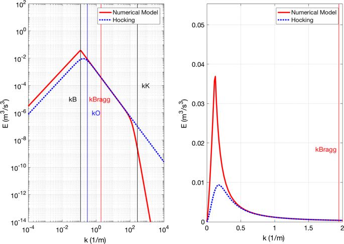
Assumed spectral shape, log scale (left) and linear (right) for \(\sigma = 0.1\) m/s and \(\varepsilon = 0.47\frac{{\sigma^{3} }}{L}\) with L = 25 m (fK = 1, N = 0.0121 s−1). These values can be changed and spectral shape replotted using the code provided. Note how the energy is concentrated at low wavenumbers, and therefore, the spectral shape in the ISR and beyond is important. Note also the difference relative to Hocking’s spectrum (Eq. 66) in the BSR and beyond
-
3.
Option “vsr”: can be put to 1, if viscous subrange is to be considered. This is seldom necessary.
-
4.
Option “wind”: value of 1 considers wind advection, although the wind velocity itself can be prescribed to be nearly zero (zero value is not permitted by the code. Use 0.0001 instead). However, wind = 0 makes integration quicker for the zero wind case.
-
5.
Option fK: the ratio between Ozmidov wavenumber and the outer scale wavenumber. It can be put equal to 1 or whatever value is found appropriate by future studies.
-
6.
Option CK: This is the constant introduced because of the nearly transverse nature of radar measurements (vertical beam in particular). See Appendix B for details.

Figure 5 shows numerical results for 4 cases (for CK = 0.873):

Non-dimensional TKE dissipation rate plotted against 2kBb. Top left: Base case with abyb = 0, Lby2b = 0.001 (zero altitude and zero wind). Top right: Case with abyb = 10, Lby2b = 0.001 (nonzero altitude). Bottom left: Case with abyb = 0, Lby2b = 5 (nonzero wind). Bottom right: Case with abyb = 10, Lby2b = 5 (nonzero altitude and wind). Solid line is the numerical model, the dotted line is Weinstock and dashed line, White et al. Hocking = 0, waves = 0 and fK = 1, and the upper limit of integrations is \(\infty\), in the above simulations. If instead Bragg wavenumber were imposed as the upper limit, the model would depart from Weinstock values at high values of kB(2b). The transition value of kB(2b) between Weinstock and White et al. formulations depends very much on the values of L/2b and 2a/2b. Because CK = 0.873 and not equal to 1, the numerical model does not asymptote exactly to the two limits (see Appendix B)
-
1.
Base case with abyb = 0, Lby2b = 0.001 (zero altitude and zero wind).
-
2.
Case with abyb = 10, Lby2b = 0.001 (altitude/beam angle dependence)
-
3.
Case with abyb = 0, Lby2b = 5 (Nonzero wind)
-
4.
Case with abyb = 10, Lby2b = 5 (Nonzero wind)
Note that White et al. formulation leads to \(\sigma^{3}\) dependence of \(\varepsilon\), and therefore, there is no dependence on kB. On the other hand, Weinstock formulation depends on N and hence kB(2b). The numerical model provides values between these two asymptotic limits and hence is useful for general use. Through suitable changes, the parameter space can be more fully explored and/or specific radar and ambient conditions explored.
Finally, the code can also compute \(\bar{\varepsilon }\) for convective conditions, where ISR is presumed to exist throughout the range of integration.
The depth of the convective layer is an independent parameter. Values for b and \(\sigma\) need to be provided to do the computation. Precise values are not important since the non-dimensional dissipation rate is not a function of these parameters. Figures 6 and 7 show results for a convective layer 500 m deep, for various values of 2a/2b and L/2b. The strong influence of these parameters suggests that the base case of zero altitude and zero winds is not the best approximation in general. Figure 6 shows results for CK = 1 and Fig. 7, for CK = 0.437.

Non-dimensional TKE dissipation rate plotted against 2a/2b, for various values of L/2b for CK = 1. Note the strong influence of these parameters

As in Fig. 6 but for CK = 0.437
For the convective case,
-
1.
Option “vsr”: can be put to 1, if viscous subrange is to be considered. This is seldom necessary.
-
2.
Option “wind”: value of 1 considers wind advection, although the wind velocity itself can be prescribed to be nearly zero (zero value is not permitted by the code. Use 0.0001 instead). However, wind = 0 makes integration quicker for the zero wind case.
-
3.
Option CK: This is the constant introduced because of the nearly transverse nature of radar measurements (vertical beam in particular). See Appendix B for details.
Appendix B: Transverse nature of radar measurements of velocity fluctuations
The vertical radar beam is transverse to the horizontal wind advecting turbulence past the radar beam, and hence, the variance of the radial velocity fluctuations measured by the radar may not be the same as the variance of vertical velocity fluctuations derived by integrating the theoretical spectrum (e.g., Eq. 41). The difference between the “parallel” spectrum (for example, spectrum measured in the direction of traverse by a sensor carried by an aircraft traversing the turbulence field), “transverse” spectrum (spectrum measured perpendicular to the direction of traverse) and the theoretical spectrum was first mentioned by Hocking (1983) and is well explained in Appendix A of Hocking (1999). Accordingly, the spectrum of velocity fluctuations parallel and transverse to the horizontal wind (in the inertial subrange) is given by:
Integrating these spectra yields
for the parallel and transverse components with respect to the horizontal wind. However, integration of conventional spectrum (Eq. 26) from kout to \(\infty\) yields
If we invoke isotropy, \(q^{2} = 3\overline{{w^{2} }}\), C1 = 1 and we get Eq. (30). Therefore,
On the other hand, if we recognize that in shear-generated turbulence, the energy is deposited by shear into the turbulence component in the direction of mean velocity and then distributed to the other two components by pressure covariance terms (see for example, Kantha and Clayson 1994, 2004), \(q^{2} \sim4\overline{{w^{2} }}\) and C1 ~ 0.75 so that
Similarly, for convective turbulence, where energy is deposited into the vertical component and then distributed to horizontal components, \(q^{2} \sim2\overline{{w^{2} }}\) and C1 ~ 1.5 so that
This means that the integrals on the right hand side of Eqs. (41), (44), (47) and (48) should include factor CK, whose value depends on the nature of turbulence and is equal to 0.873 for turbulence in stably stratified flows, and 0.437 for convective turbulence. The expressions for \(\varUpsilon\) in Eqs. (46), (50), (51), (54), (58) and \(\overline{\varUpsilon }\) in Eqs. (62) and (63) should also include the same factor as well. The corresponding estimates of TKE dissipation rate \(\varepsilon\) and \(\overline{\varepsilon }\) would increase by a factor of (1/0.873)3/2 ~ 1.23, and (1/0.437)3/2 ~ 3.46, respectively.
Remarkably, the fact that the radar beam is transverse to the wind, and hence, \(\sigma^{2}\) may not be equal to \(\overline{{w^{2} }}\) obtained by integrating the TKE spectrum appears to have been unrecognized so far (to our knowledge anyway) in the derivations of expressions for \(\sigma^{2}\) in radar literature. However, it is important to note that the transverse nature of vertical radar beam measurements may be diluted by the fact that the radar averages vertical fluctuations over the measurement volume (personal communication from Prof. Wayne Hocking). While the horizontal dimension of the radar beam introduces some averaging in the horizontal direction, the vertical beam still makes essentially a transverse measurement, since it is taking averages of a bunch of transverse measurements adjacent to one another. The value of CK may be closer to 0.873 (and 0.437 for convection) than 1.0, but because of many other uncertainties involved, the precise value is not that easy to ascertain at present. Further calibration measurements are essential to pin down the value of CK (personal communication from Prof. Wayne Hocking). The code has provisions to prescribe the appropriate multiplication factor CK, whether by invoking conventional approach or by allowing for the transverse nature. However, the precise value awaits further research and confirmation of the transverse nature of radar measurements.
The numerical code will be submitted as Additional file 1.
Rights and permissions
Open Access This article is distributed under the terms of the Creative Commons Attribution 4.0 International License (http://creativecommons.org/licenses/by/4.0/), which permits unrestricted use, distribution, and reproduction in any medium, provided you give appropriate credit to the original author(s) and the source, provide a link to the Creative Commons license, and indicate if changes were made.
About this article

Cite this article
Kantha, L., Luce, H. & Hashiguchi, H. On a numerical model for extracting TKE dissipation rate from very high frequency (VHF) radar spectral width. Earth Planets Space 70, 205 (2018). https://doi.org/10.1186/s40623-018-0957-7
Received:
Accepted:
Published:
DOI: https://doi.org/10.1186/s40623-018-0957-7