
Abstract
The input to a machine learning model is a one-dimensional feature vector. However, in recent learning models, such as convolutional and recurrent neural networks, two- and three-dimensional feature tensors can also be inputted to the model. During training, the machine adjusts its internal parameters to project each feature tensor close to its target. After training, the machine can be used to predict the target for previously unseen feature tensors. What this study focuses on is the requirement that feature tensors must be of the same size. In other words, the same number of features must be present for each sample. This creates a barrier in processing images and texts, as they usually have different sizes, and thus different numbers of features. In classifying an image using a convolutional neural network (CNN), the input is a three-dimensional tensor, where the value of each pixel in each channel is one feature. The three-dimensional feature tensor must be the same size for all images. However, images are not usually of the same size and so are not their corresponding feature tensors. Resizing images to the same size without deforming patterns contained therein is a major challenge. This study proposes zero-padding for resizing images to the same size and compares it with the conventional approach of scaling images up (zooming in) using interpolation. Our study showed that zero-padding had no effect on the classification accuracy but considerably reduced the training time. The reason is that neighboring zero input units (pixels) will not activate their corresponding convolutional unit in the next layer. Therefore, the synaptic weights on outgoing links from input units do not need to be updated if they contain a zero value. Theoretical justification along with experimental endorsements are provided in this paper.
Introduction
Convolutional neural network (CNN) has recently outperformed other neural network architectures, machine learning, and image processing approaches in image classification [6, 46, 50, 56, 58] due to its independence from hand-crafted visual features and excellent abstract and semantic abilities [58]. CNN makes strong and mostly correct assumptions about the nature of images, namely, locality of pixel dependencies and stationarity of statistics. Therefore, in comparison with standard feed-forward neural networks, CNN has much fewer connections and parameters which makes it easier to train.
A CNN consists of convolutional layers followed by fully-connected layers (Fig. 1). A convolutional layer consists of a convolution filter, followed by a pooling filter and an activation function. A convolution filter has a number (n) of filters, with the same window size (f), sweeping over the image with a stride of sf. Pooling summarizes the outputs of neighboring groups of neurons in the same kernel map. A pooling layer has a window with the size of p that sweeps over the image with a stride of sp. A common pooling function is the maximum pooling function which outputs the maximum value in the kernel map [25] and is utilized in our model. The last fully-connected layer in CNN has as many neurons as the number of classes. Among the model’s hyperparameters are n, f, sf, p, sp and the number of neurons in fully-connected layers.

A typical architecture for CNN
The convolution filter and the pooling filter would slip outside the input image into the void, when they attempt to center themselves at bordering pixels. There are two strategies to solve this issue: (a) stopping the filter before it slips outside the image and (b) padding the input image with zero pixels. The first approach comes at the cost of under-scanning the bordering pixels because the filter will not get a chance to center itself at the bordering pixels. The second approach is referred to as padding and is the one applied in our model.
Since neural networks receive inputs of the same size, all images need to be resized to a fixed size before inputting them to the CNN [14]. The larger the fixed size, the less shrinking required. Less shrinking means less deformation of features and patterns inside the image. This will mitigate the classification accuracy degradation due to deformations. However, large images not only occupy more space in the memory but also result in a larger neural network. Thus, increasing both the space and time complexity. It is obvious now that choosing this fixed size for images is a matter of tradeoff between computational efficiency and accuracy.
Images larger than the fixed size (in one dimension or both) could be resized down to the desired fixed size using two approaches: cropping their border pixels or scaling them down using interpolation. Both approaches are lossy. While cropping poses the risk of missing the features or patterns that appear in border areas, scaling poses the risk of deforming features or patterns across the image. Since deforming patterns is less risky than losing them, scaling is the reasonable choice to resize larger images down to the desired fixed size. Resizing smaller images up to the fixed size is the focus of this study. Zero-padding is proposed for this purpose and compared with the conventional approach of scaling images up (zooming in) using interpolation.
Related works
Despite their emergence in the late 1980s, CNNs were still dormant in visual tasks until the mid-2000s. The increase in computing power, large amounts of labeled data, and algorithmic innovations brought CNNs to the forefront of visual tasks. CNNs overcome the formidable tasks of feature extraction and transformation, as well as pattern analysis and classification, by exploiting multiple layers of nonlinear information processing [15].
Krizhevsky et al. [25] used a CNN to classify 1.2 million images into 1000 classes in the ImageNet Large Scale Visual Recognition Challenge (ILSVRC) 2012. They won this challenge with record-breaking results and marked the most significant advance for image classification tasks. Ever since, CNNs have dominated the image classification component of subsequent versions of the ILSVRC [17, 39, 41, 46, 58].
Zeiler and Fergus [58] used a multilayered deconvolutional network [59] to understand the intermediate feature extraction layers of the network. They used this in a diagnostic role to derive ways to improve CNN architecture and performance. Their model outperformed Krizhevsky et al. [25] on the ImageNet classification benchmark and won the ILSVRC 2013 [39]. Their model also achieved the best published results on the CALTECH-101 [7] and CALTECH-256 data sets [13].
A CNN architecture, called Inception, was introduced by Szegedy et al. [46]. GoogLeNet model consisting of 22 layers, inspired by the Inception architecture, won both the ImageNet classification and detection challenges in 2014 [39]. Such a large network with a large number of parameters is not only computationally burdensome to train, but also susceptible to overfitting. To overcome these challenges, they reduced the number of connections in their network based on Hebbian principles to create a sparsely connected convolutional architecture, rather than a fully connected one. More specifically, they used 1 × 1 convolutions as dimension-reduction blocks prior to 3 × 3 and 5 × 5 convolutions. This allowed them to increase the network size without exponentially increasing the computational cost. Simonyan and Zisserman [41] also used a deep CNN with 19 layers in the ILSVRC 2014 classification contest [39]. Instead of the Inception model, arguing that it is too complex, they used smaller-sized convolutional filters (3 × 3) across the CNN and kept the parameters constant.
The winner of the ILSVRC 2015 [39] was a CNN with 152 layers, developed by He et al. [17]. They applied a residual learning framework to overcome the difficulty of training their deep network. To make it easier to optimize and train, they allowed errors to be propagated directly to the preceding units. This was realized by forcing the layers of the network to learn residual functions with reference to their preceding layer inputs rather than learning unreferenced functions. They also found that optimized residual modules worked more optimally than their initial residual module configurations. Table 1 lists other recent attempts to improve different aspects of CNNs.
Since the emergence of CNNs and their staggering success in image classification, many attempts have been made by researchers to improve their accuracy and time performance. These improvements have targeted different aspects of CNNs, including network architecture, activation functions, regularization mechanisms, and optimization techniques among others. However, one aspect that has not witnessed much attention is the strict requirement of CNNs in receiving images of the same size. In other words, resizing all images to a fixed size is a prerequisite for classifying them using CNN. While interpolation has been widely and traditionally used to scale all the images to the same size, alternative options for doing so has not been sufficiently explored. Therefore, this study is devoted to this aspect of CNNs.
Zero-padding vs. scaling up using interpolation
As shown in Fig. 2, there are two approaches to resize smaller images up to the fixed size: zero-padding and scaling them up (zooming in) using interpolation. Zero-padding has two advantages in comparison with scaling. The first advantage is that while scaling carries the risk of deforming the patterns in the image, padding does not. The second advantage of zero-padding is that it speeds up the calculations, in comparison with scaling, resulting in better computational efficiency. The reason is that neighboring zero input units (pixels) will not activate their corresponding convolutional unit in the next layer. Therefore, the synaptic weights on outgoing links from input units do not need to be updated if they contain a zero value. This is similar to a dropout that only concerns border pixels in the input layer. This advantage will be lost if smaller images are enlarged by increasing their resolution (scaling) rather than zero-padding.

A small image (a) resized to 200 × 200 pixels using zero-padding (b) and interpolation (c)
In the following we invalidate two plausible disadvantages of zero-padding in comparison with scaling:
Since smaller images are enlarged by adding zero-value pixels around their borders, the CNN will not sufficiently learn to extract features from the border areas, as well as it learns to do so in central areas. In other words, the synaptic weights on links from the border pixels to the first convolutional layer will not have the opportunity to be sufficiently trained because the input value for border pixels is zero for many images. This assumption is not true as the weight sharing property of CNN uses the same synaptic weights over all convolution windows. Figure 3 depicts the convolution window that sweeps across the image and the fact that the synaptic weights (a, b, c, d, e, f, g, h, and i) are the same for all convolution windows. In other words, the CNN’s power in extracting features from the border areas of an image is equal to its power in extracting features from the central areas.
Fig. 3 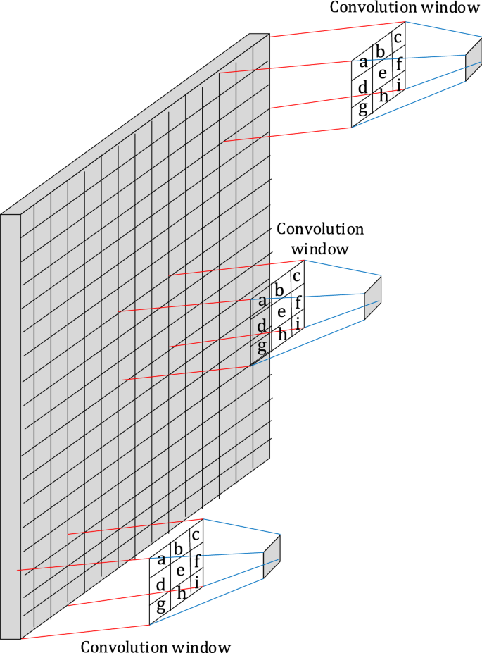
Synaptic weights (a, b, c, d, e, f, g, h, and i) are the same for all convolution windows in CNN
The forged zero-value pixels around smaller images will adversely disturb the optimization of synaptic weights. This assumption is not true because zero-value pixels will not activate during forward and backward propagation. In other words, zero-value input units will not contribute to the forward pass and their corresponding synaptic weights will not be updated during the backpropagation. Following is the mathematical proof:

Proof
In the backpropagation algorithm [3, 16, 52], the architecture of the network is fixed and its synaptic weights (W) are computed so as to minimize a cost function defined as:
where N is the number of training samples and ε(i) is a function of the network’s output (\(\hat{y}\left( i \right)\)) and the desired output (y(i)) for the i-th training sample. We can iteratively find the synaptic weight vectors that minimize the perceptron cost function using the gradient descent scheme [3, 16, 52]. In each iteration, the weight vector (including the threshold) of the j-th node in the r-th layer (\(\varvec{w}_{j}^{r}\)) is modified through Eq. 2:
The modification term in Eq. 2 (\(\Delta \varvec{w}_{j}^{r}\)) is computed through Eq. 3 according to the gradient descent scheme, where α is referred to as the training rate:
By substituting the cost function from Eq. 1 in Eq. 3 and applying the chain rule in differentiation, we obtain:
where \(v_{j}^{r} \left( i \right)\) is the value at the jth node in the rth layer before the activation function is applied to it. By defining \(\delta_{j}^{r} \left( i \right) = \frac{\partial \varepsilon \left( i \right)}{{\partial v_{j}^{r} \left( i \right)}}\) in the above equation, we obtain:
We can calculate \(\frac{{\partial v_{j}^{r} \left( i \right)}}{{\partial \varvec{w}_{j}^{r} }}\) using Eq. 6 as follows:
where kr-1 is the number of nodes in the (r − 1)th layer and \(\hat{y}^{r - 1} \left( i \right)\) is the output vector of the (r − 1)th layer for the ith training sample. By substituting Eq. 6 in Eq. 5 we obtain:
Considering that \(\varvec{w}_{j}^{r}\) in the above equation is the weight vector of the jth node in the rth layer, we can calculate \(w_{jk}^{r}\), the synaptic weight from the kth node at the (r − 1)th layer to the jth node at the rth layer, as:
We needed to prove that the synaptic weights from a node in the first layer to another node in the second layer will not be updated if the value of the node in the first layer is zero. This is equivalent to proving that \(\Delta w_{jk}^{r}\) is zero if \(\hat{y}_{k}^{r - 1} \left( i \right)\) is zero. Equation 8 proves this, because if we replace \(\hat{y}_{k}^{r - 1} \left( i \right)\) with zero in Eq. 8, it will result in zero for \(\Delta w_{jk}^{r}\). This proof is independent from the choice of the activation functions or the cost function, ε(i). \(\square\)
In the next section, two experiments are conducted with publicly available datasets to verify the faster training of zero-padding in comparison with scaling up smaller images using interpolation to the desired fixed size.
Experiments
CNN setup
AlexNet [25], an 8-layer deep architecture for CNN, is applied here. This architecture entails 5 convolutional layers followed by 3 fully-connected layers, as shown in Fig. 4. The following settings are considered for the convolutional layers: f1 = 11 × 11 × 3, s1 = 4, n1 = 96, f2 = 5 × 5 × 96, s2 = 1, n2 = 256, f3 = 3 × 3 × 256, s3 = 1, n3 = 384, f4 = 3 × 3 × 384, s4 = 1, n4 = 384, f5 = 3 × 3 × 384, s5 = 1, n5 = 256, where fm, sm, and nm denote the size, stride, and number of filters of the m-th layer respectively. The first two fully-connected layers have 4096 neurons each and the third fully-connected layer has as many neurons as the number of classes.

AlexNet architecture in our application
The last fully-connected layer is followed by an n-way softmax function which produces a probability distribution over the n class labels. The softmax function in the final layer, softmax(zi) = exp(zi)/Ʃj exp(zj), transforms the values (xi) to normalized exponential probabilities whose summation is one (i.e. Ʃc pc = 1). This provision (Ʃc pc = 1) is a prerequisite for the application of cross-entropy loss function. The cross-entropy loss function is computed as: − Ʃc yc log(pc), where c represents a class (or neuron) in the final layer, yc stands for the desired output value (0 or 1) at that neuron, and pc for the predicted probability at that neuron. The Adam optimization algorithm [24] is used to train the network. It is an extension to the stochastic gradient descent (SGD) approach. As opposed to SGD’s single and fixed learning rates for all synaptic weight updates, Adam continually adjusts individual adaptive learning rates for each synaptic weight based on estimates of first and second moments of the gradients. We initialized the learning rate at 0.0001 and the exponential decay rate for the first and second moment estimates at 0.9 and 0.999 respectively. These values are suggested by Kingma and Ba [24].
Pooling function is in charge of summarizing the outputs of neighboring groups of neurons in the same kernel map. A size of 3 × 3 and stride of 2 are considered for pooling layers, proposed by Zeiler and Fergus [57] and Krizhevsky et al. [25]. Larger pooling regions are too noisy during training and smaller regions cause over-fitting [57]. The stride being smaller than the size of the pooling region causes the pooling regions to overlap. Overlapping pooling can improve the generalization accuracy by reducing overfitting [25]. Pooling layers in our network follow the first, second, and fifth convolutional layers. Maximum pooling function, which is conventionally used in AlexNet [25], outputs the maximum value in the kernel map. It is also applied in our model.
Rectified Linear Unit (ReLU) [21, 35], defined as the positive part of its argument: ReLU(z) = max(0,z), is a piecewise linear function. It is commonly used as activation function at all layers, except the last one, where a softmax function is preferred to produce a probability distribution over the class labels.
Datasets
Two datasets from http://www.image-net.org are used here: Tiny Imagenet (Stanford CS231N) and Visual Domain Decathlon (PASCAL in Detail Workshop Challenge). Tiny Imagenet is similar to the classification in the full ImageNet challenge (ILSVRC) but with a smaller dataset. Tiny Imagenet contains 200 classes. Each class has 500 training images and 50 validation images. The test set contains 10,000 images. All images are 64 × 64 colored ones. Visual Domain Decathlon contains 1000 classes. Each class has 1250 training images and 50 validation images. The test set contains 50,000 images. All images are colored and image sizes range from 72 × 72 to 72 × 1125. The average number of pixels in an image is 7155 and the median is 6912.
Results and discussion
The experiments were implemented in TensorFlow package in Python and run on a 2.60 GHz Intel Xeon CPU E5-2670M, 20 M cash size, and 350G RAM. All images are resized to 224 × 224 pixels. Without extra preprocessing, the image pixels are only divided by 255 so that they are in the range 0 to 1. In each experiment, 20% of images are held out for testing. A tenfold cross validation is performed using the remaining 80% of labeled images to find the optimal number of training epochs. The stop epoch is the smallest epoch whose tenfold cross-validation accuracy falls within one standard deviation of the best. After finding the optimal stop epoch, the machine is trained using the entire 80% of the data and then tested using the 20% of the data which were primarily held out of the ten-fold cross-validation.
The classification accuracy was not impacted by the choice of the approach for resizing small images up to the fixed size. Zero-padding reduced the training time per epoch by 3% on average for the first dataset and 11% for the second dataset. This is an experimental endorsement of the theoretical justification presented for this approach in the previous section.
A more detail investigation showed that the reduction in training time is proportional to: (a) the number of images which at least one of their dimensions is smaller than the fixed size and (b) the amount of zero-padding required to get the smaller images up to the fixed size. These two factors are mainly responsible for the larger training time reduction in the second dataset.
Conclusions and future directions
Since the emergence of CNNs and their staggering success in image classification, many attempts have been made by researchers to improve their accuracy and time performance. These improvements have targeted different aspects of CNNs, including network architecture, activation functions, regularization mechanisms, and optimization techniques among others. However, one aspect that has not witnessed much attention is the strict requirement of CNNs in receiving images of the same size. In other words, resizing all images to a fixed size is a prerequisite for classifying them using CNN. While interpolation has been widely and traditionally used to scale all the images to the same size, alternative options for doing so has not been sufficiently explored. With that in mind, this study proposed zero-padding around smaller images, as opposed to interpolation, to resize them up to the fixed size. Zero-padding has no effect on the classification accuracy but considerably reduces the training time. The reason is that neighboring zero input units (pixels) will not activate their corresponding convolutional unit in the next layer. Therefore, the synaptic weights on outgoing links from input units do not need to be updated if they contain a zero value. While zero-padding and interpolation bypass the problem of multi-resolution image classification by resizing smaller images to a fixed size, our future work focuses on classifying multi-resolution images without resizing them. This will require some reforms in CNN itself.
Availability of data and materials
Not applicable.
Abbreviations
- CNN:
-
convolutional neural network
- ILSVRC:
-
ImageNet Large Scale Visual Recognition Challenge
- ReLU:
-
rectified linear unit
- LReLU:
-
leaky rectified linear unit
- PReLU:
-
parametric rectified linear unit
- APL:
-
adaptive piecewise linear
- RReLU:
-
randomized rectified linear unit
- ELU:
-
exponential linear unit
- SReLU:
-
s-shaped rectified linear unit
- SGD:
-
stochastic gradient descent
References
Agostinelli F, Hoffman M, Sadowski P, Baldi, P. Learning activation functions to improve deep neural networks. 2014. arXiv preprint, arXiv:1412.6830.
Ba J, Frey B. Adaptive dropout for training deep neural networks. In: Burges CJ, Bottou L, Welling M, Ghahramani Z, Weinberger KQ, editors. Advances in neural information processing systems, vol. 26. Red Hook: Curran; 2013. p. 3084–92.
Bishop CM. Neural networks for pattern recognition. Oxford: Oxford University Press; 1995.
Clevert D-A, Unterthiner T, Hochreiter S. Fast and accurate deep network learning by exponential linear units (ELUs). In: Proceedings of the 4th international conference on learning representations. 2016. p. 1–14.
Collobert R, Bengio S. A gentle Hessian for efficient gradient descent. In: Proceedings of the IEEE international conference on acoustics, speech, and signal processing. 2004. p. 517–20.
Farfade SS, Saberian MJ, Li L-J. Multi-view face detection using deep convolutional neural networks. In: 5th international conference on multimedia retrieval. New York: ACM. 2015. p. 643–50.
Fei-Fei L, Fergus R, Perona P. One-shot learning of object categories. IEEE Trans Pattern Anal Mach Intell. 2006;28(4):594–611.
Glorot X, Bengio Y. Understanding the difficulty of training deep feedforward neural networks. In: Proceedings of the 13th international conference on artificial intelligence and statistics. 2010. p. 249–56.
Gong Y, Wang L, Guo R, Lazebnik S. Multi-scale orderless pooling of deep convolutional activation features. In: Proceedings of the European conference on computer vision. Berlin: Springer; 2014. p. 392–407.
Goodfellow IJ, Warde-Farley D, Mirza M, Courville A, Bengio Y. Maxout networks. In: Proceedings of the 30th international conference machine learning. 2013. p. 1319–27.
Graham B. Fractional max-pooling. 2014. arXiv preprint, arXiv:1412.6071.
Grauman K, Darrell T. The pyramid match kernel: discriminative classification with sets of image features. In: Proceedings of the IEEE international conference on computer vision. Red Hook: Curran; 2005. p. 1458–65.
Griffin G, Holub A, Perona P. Caltech-256 object category dataset. Pasadena: California University of Technology; 2007.
Hashemi M. Web page classification: a survey of perspectives, gaps, and future directions. Multimed Tools Appl. 2019. https://doi.org/10.1007/s11042-019-08373-8.
Hashemi M, Hall M. Detecting and classifying online dark visual propaganda. Image Vis Comput. 2019;89(1):95–105.
Haykin SS. Neural networks: a comprehensive foundation. 2nd ed. Upper Saddle River: Prentice Hall; 1999.
He K, Zhang X, Ren S, Sun J. Delving deep into rectifiers: surpassing human-level performance on imagenet classification. In: Proceedings of the IEEE international conference on computer vision. Red Hook: Retrieved from Curran; 2015. p. 1026–34.
He K, Zhang X, Ren S, Sun J. Spatial pyramid pooling in deep convolutional networks for visual recognition. IEEE Trans Pattern Anal Mach Intell. 2015;37(9):1904–16.
He K, Zhang X, Ren S, Sun J. Deep residual learning for image recognition. In: Proceedings of the ieee conference on computer vision and pattern recognition. 2016. p. 770–8.
He K, Zhang X, Ren S, Sun J. Identity mappings in deep residual networks. European conference on computer vision. Cham: Springer; 2016. p. 630–45.
Hinton GE, Srivastava N, Krizhevsky A, Sutskever I, Salakhutdinov RR. Improving neural networks by preventing co-adaptation of feature detectors. 2012. arXiv preprint, arXiv:1207.0580.
Huang G, Liu Z, Maaten LV, Weinberger KQ. Densely connected convolutional networks. In: Proceedings of the IEEE conference on computer vision and pattern recognition. 2017. p. 4700–8.
Jin X, Xu C, Feng J, Wei Y, Xiong J, Yan S. Deep learning with s-shaped rectified linear activation units. In: 13th AAAI conference on artificial intelligence. 2016.
Kingma DP, Ba J. Adam: a method for stochastic optimization. 2014. arXiv preprint, arXiv:1412.6980.
Krizhevsky A, Sutskever I, Hinton GE. Imagenet classification with deep convolutional neural networks. In: Advances in Neural information processing systems. 2012. p. 1097–105.
Laptev D, Savinov N, Buhmann JM, Pollefeys M. TI-POOLING: transformation-invariant pooling for feature learning in convolutional neural networks. In: Proceedings of the IEEE conference on computer vision and pattern recognition. 2016. p. 289–97.
Lazebnik S, Schmid C, Ponce J. Beyond bags of features: Spatial pyramid matching for recognizing natural scene categories. In: Proceedings of the IEEE conference on computer vision and pattern recognition. Red Hook: Curran; 2006. p. 2169–78.
Lee C-Y, Gallagher PW, Tu Z. Generalizing pooling functions in convolutional neural networks: mixed, gated, and tree. In: Proceedings of the 19th international conference on artificial intelligence and statistics. 2016. p. 464–72.
Li Z, Gong B, Yang T. Improved dropout for shallow and deep learning. In: Lee D, Sugiyama M, Luxburg UV, Guyon I, Garnett R, editors. Advances in neural information processing systems. 2016. p. 2523–31.
Lin M, Chen Q, Yan S. Network in network. 2013. arXiv preprint, arXiv:1312.4400.
Liu W, Wen Y, Yu Z, Yang M. Large-margin softmax loss for convolutional neural networks. In: Proceedings of the 33rd international conference machine learning, vol. 2. 2016. p. 507–16.
Maas AL, Hannun AY, Ng AY. Rectifier nonlinearities improve neural network acoustic models. In: Proceedings of the 30th international conference machine learning, vol. 30. 2013. p. 1–8.
Mishkin D, Matas J. All you need is a good init. In Proceedings of the 4th international conference on learning representations. 2016. p. 1–13.
Nagi J, Caro GA, Giusti A, Nagi F, Gambardella LM. Convolutional neural support vector machines: hybrid visual pattern classifiers for multi-robot systems. In: Proceedings of the 11th international conference on machine learning and applications. Los Alamitos: IEEE; 2012. p. 27–32.
Nair V, Hinton GE. Rectified linear units improve restricted boltzmann machines. In: The 27th international conference on machine learning. 2010. p. 807–14.
National Data Science Bowl | Kaggle. 2016. https://www.kaggle.com/c/datasciencebowl.
Rippel O, Gelbart M, Adams R. Learning ordered representations with nested dropout. In: Proceedings of the 30th international conference on machine learning. 2014. p. 1746–54.
Rippel O, Snoek J, Adams RP. Spectral representations for convolutional neural networks. In: Cortes C, Lawrence ND, Lee DD, Sugiyama M, Garnett R, editors. Advances in neural information processing systems, vol. 28. Red Hook: Curran; 2015. p. 2449–57.
Russakovsky O, Deng J, Su H, Krause J, Satheesh S, Ma S, Huang Z, Karpathy A, Khosla A, Bernstein M, Berg AC. ImageNet large scale visual recognition challenge. Int J Comput Vis. 2015;115(3):211–52.
Sermanet P, Chintala S, LeCun Y. Convolutional neural networks applied to house numbers digit classification. In: Proceedings of the 21st international conference on pattern recognition. Red Hook: Curran; 2012. p. 3288–91.
Simonyan K, Zisserman A. Very deep convolutional networks for large-scale image recognition. 2014. arXiv preprint, arXiv:1409.1556.
Springenberg JT, Riedmiller M. Improving deep neural networks with probabilistic maxout units. 2013. arXiv preprint, arXiv:1312.6116.
Srivastava NG, Krizhevsky A, Sutskever I, Salakhutdinov R. Dropout: a simple way to prevent neural networks from overfitting. J Mach Learn Res. 2014;15(1):1929–58.
Srivastava RK, Greff K, Schmidhuber J. Training very deep networks. In: Cortes C, Lawrence ND, Lee DD, Sugiyama M, Garnett R, editors. Advances in neural information processing systems, vol. 28. Red Hook: Curran; 2015. p. 2377–85.
Srivastava RK, Greff K, Schmidhuber J. Highway networks. 2015. arXiv preprint, arXiv:1505.00387.
Szegedy C, Liu W, Jia Y, Sermanet P, Reed S, Anguelov D, Erhan D, Vanhoucke V, Rabinovich A. Going deeper with convolutions. In: IEEE conference on computer vision and pattern recognition. New York: IEEE; 2015. p. 1–9.
Szegedy C, Vanhoucke V, Ioffe S, Shlens J, Wojna Z. Rethinking the Inception architecture for computer vision. In: Proceedings of the IEEE conference on computer vision and pattern recognition. 2016. p. 2818–26.
Tompson J, Goroshin R, Jain A, LeCun Y, Bregler C. Efficient object localization using convolutional networks. In: Proceedings of the IEEE conference on computer vision and pattern recognition. Los Alamitos: IEEE; 2015. p. 648–56.
Wan L, Zeiler M, Zhang S, Cun YL, Fergus R. Regularization of neural networks using Dropconnect. In: Proceedings of the 30th international conference machine learning. 2013. p. 1058–66.
Wang M, Liu X, Wu X. Visual classification by l1-hypergraph modeling. IEEE Trans Knowl Data Eng. 2015;27(9):2564–74.
Wang S, Manning C. Fast dropout training. In: Proceedings of the 30th international conference on machine learning. 2013. p. 118–26.
Werbos PJ. Beyond regression: new tools for prediction and analysis in the behavioral sciences. Cambridge: Ph.D. Thesis, Harvard University; 1974.
Wu H, Gu X. Max-pooling dropout for regularization of convolutional neural networks. In: Proceedings of the 22nd international conference neural information processing. Berlin: Springer; 2015. p. 46–53.
Yang J, Yu K, Gong Y, Huang TS. Linear spatial pyramid matching using sparse coding for image classification. In: Proceedings of the IEEE conference on computer vision and pattern recognition, vol. 1. Red Hook: Curran; 2009. p. 1794–801.
Yu D, Wang H, Chen P, Wei Z. Mixed pooling for convolutional neural networks. In: Proceedings of the 9th international conference on rough sets and knowledge technology. Berlin: Springer; 2014. p. 364–75.
Yu J, Tao D, Wang M. Adaptive hypergraph learning and its application in image classification. IEEE Trans Image Process. 2012;21(7):3262–72.
Zeiler MD, Fergus R. Stochastic pooling for regularization of deep convolutional neural networks. 2013. arXiv preprint, arXiv:1301.3557.
Zeiler MD, Fergus R. Visualizing and understanding convolutional networks. In: European conference on computer vision. Berlin: Springer; 2014. p. 818–33.
Zeiler MD, Taylor GW, Fergus R. Adaptive deconvolutional networks for mid and high level feature learning. In: Proceedings of the IEEE international conference on computer vision, vol. 1. Red Hook: Curran; 2011. p. 2018–25.
Zhai S, Cheng Y, Zhang ZM, Lu W. Doubly convolutional neural networks. In: Lee D, Sugiyama M, Luxburg UV, Guyon I, Garnett R, editors. Advances in neural information processing systems. vol. 29. 2016. p. 1082–90.
Acknowledgements
Not applicable.
Funding
Not applicable.
Author information
Authors and Affiliations
Contributions
The author read and approved the final manuscript.
Corresponding author
Ethics declarations
Competing interests
The author declares no competing interests.
Additional information
Publisher's Note
Springer Nature remains neutral with regard to jurisdictional claims in published maps and institutional affiliations.
Rights and permissions
Open Access This article is distributed under the terms of the Creative Commons Attribution 4.0 International License (http://creativecommons.org/licenses/by/4.0/), which permits unrestricted use, distribution, and reproduction in any medium, provided you give appropriate credit to the original author(s) and the source, provide a link to the Creative Commons license, and indicate if changes were made.
About this article

Cite this article
Hashemi, M. Enlarging smaller images before inputting into convolutional neural network: zero-padding vs. interpolation. J Big Data 6, 98 (2019). https://doi.org/10.1186/s40537-019-0263-7
Received:
Accepted:
Published:
DOI: https://doi.org/10.1186/s40537-019-0263-7