
Abstract
Energy-hungry data centers attract researchers’ attention to energy consumption minimization–a challenge confronted by both industry and academia. To assure the server reliability, its instantaneous temperature is generally controlled within a preset threshold. Nonetheless, field studies indicated that the occasional violation of extreme temperature constraints hardly affect the system reliability in practice. Therefore, strictly restraining the server temperature may contribute to meaningless energy consumption. As a response to this limitation, this paper presents a dynamic control algorithm without violating the average temperature constraint. We formulate a “soft” Server Temperature-Constrained Energy Minimization (STCEM) problem, where the object function consists of IT and Heat Ventilation & Air Conditioner (HVAC) energy. Based on the Lyapunov optimization, two algorithms, i.e., linear and quadratic control policies, are proposed to approximately solve the STCEM problem. The non-negative weight parameter V is introduced to trade off the energy consumption against server temperature constraint. Furthermore, extensive simulations have been carried out to evaluate the system performance for the proposed controlled algorithms. The experimental results demonstrate that the quadratic control policy outperforms the linear counterpart on the STCEM problem. Specifically, the energy consumption and server temperature constraint are well balanced when V≈5000.
Introduction
Data center is a large-scale distributed system, where Information Technology (IT) and cooling subsystems compose a complex and massive structure. It provides user-friendly, reliable, and flexible services for various Internet applications, and it has been one of the sustentacular technologies that push IT industry forward. However, with the prevalence of cloud computing, the problem of energy consumption hiding behind convenient services gradually arose, and the situation is getting more and more serious. For a typical data center, the daily energy consumption is as much as 25,000 households, which is 100 to 200 times more than an office with the same space [1]. In 2015, up to 2.3 billion KWh electricity was consumed by the Microsoft data center located in USA, which is the third largest energy consumer among US enterprises (https://news.microsoft.com/download/presskits/cloud/docs/CloudFS.docx). In addition, as an energy-hungry system, gigantic-scale data centers not only lead to tremendous energy consumption, but also give rise to a battery of related problems, such as air pollution, water contamination, and soil destruction, etc.
It has been widely accepted that the data center consists of a number of interactive subsystems, of which the most energy-hungry components are IT and cooling subsystems. Energy consumed by IT equipments is primarily used to process service request and dissipates in the form of heat. The cooling facilities remove heat to ensure the health of IT equipment, so these two components are coupled via heat. There are a number of studies separately dealing with energy minimization in data centers. For example, [2–6] studied IT energy consumption, others [7–9] inclined to optimize cooling energy consumption. However, the aforementioned studies only concentrated on the energy consumption of a subset of system components and overlooked the interactions among them. To address this issue, joint optimization techniques [10–12], which aim to minimize the overall energy consumption, are proposed.
Nevertheless, most existing approaches either neglected the temperature constraint or ensured the server reliability by imposing a “hard” server temperature. By “hard”, it means that the server temperature must be strictly lower than a predefined threshold at all times. But actually, IT equipment is more durable than estimated. Zhang et al. [13] demonstrated that the performance and reliability of IT equipment is not greatly undermined under higher ambient temperature. Pervila et al. [14] placed computer facilities in a harsh outdoor environment, and results showed that servers can still function well when the outside temperature fluctuates dramatically. Thus, the “hard” temperature constraint underestimated the capability of failure tolerance for servers. In practice, the server temperature can occasionally exceed the preset threshold as long as the average temperature falls into a safe operating range. Using the “hard” temperature constraint, it may be too pessimistic and induce unnecessary energy consumption.
In this work, we formulate a “soft” Server Temperature-Constrained Energy Minimization (STCEM) problem. Since the system is running in a stochastic environment, to solve the STCEM problem is not an easy task. To address this issue, we leverage the Lyapunov Optimization (LO) theory to design two approximation algorithms, i.e., linear and quadratic control policies, to obtain the near-optimal solution. More specifically, we introduce virtual queues for the average temperature constraints. By guaranteeing the mean rate stability of virtual queues, the “soft” server temperature constraints are enforced [15]. To verify the efficiency of the proposed policies, we use real-world workloads [16] to run extensive simulations, and conduct detailed analysis of total and component energy efficiency. In the process, some interactive metrics, including server temperature, supplying cold air temperature, the number of powered-on servers, and Power Usage Efficiency (PUE), are carefully dissected by a series of comparison studies under two different control policies. Simulation results persuasively reveal that our proposed approach can effectively cut down the data center energy consumption. In particular, the quadratic control policy outperforms the linear control policy in terms of both energy consumption and average server temperature.
Related works
Typically, the dominant energy consumers in the data center are IT subsystem and cooling subsystem, which account for 56% and 30% of total energy, respectively [17]. In this section, we elaborate state-of-the-art IT and thermal management techniques for data center energy minimization. Since IT and cooling systems interact via heat, we also discuss the thermal model and supplying air temperatures in the data center.
IT subsystem management
To meet the Quality of Service (QoS) required by cloud users in the context of fluctuating IT workloads, data center operators usually over-provision the computing resource according to the peak workload. As a result, the IT resource is extremely underutilized (20−30% [18] in typical data centers). Staggeringly, server energy consumption is out of proportion to its utilization, and energy consumed by an idle server is about 60% of a fully utilized counterpart [19]. Controlling the sleep/active state of servers is proved to be an effective way to save IT energy. Meisner et al. [19] presented an energy conservation approach named PowerNap, which switches the operation state of servers between active and sleep modes to cater for the fluctuating workload. However, when the actual idle interval is less than the wake-up latency, the frequent switch between active and sleep modes may be negative for energy saving. To address this issue, Duan et al. [20] proposed a prediction scheme, which dynamically estimates the length of CPU idle interval and thereby intelligently picks out the most cost-efficient operation mode to effectively cut down idle energy.
Another approach to improve energy efficiency for the IT subsystem is Dynamic Voltage and Frequency Scaling (DVFS), which reduces energy consumption by dynamically scaling the supplied voltages and adjusting the CPU frequency (according to the CPU workload). Many existing researches have attained some advancement in energy-efficient scheduling by leveraging DVFS technology. To optimize the energy efficiency, some studies focused on calculating the optimal CPU frequency and controlling the supply voltage, e.g., [21–23], in which several scheduling algorithms are designed and evaluated to find the optimal frequency. Moreover, applying the Virtual Machine (VM) migration and consolidation techniques into DVFS management is an extended solution. For example, Takouna and Meinel [24] made use of the memory DVFS mechanism for VMs consolidation to cut down the energy consumption. Arroba et al. [25] proposed a DVFS-aware consolidation policy, which can consider the processor frequency when workload is dynamically allocated to servers. It is demonstrated that up to 39.14% energy is saved by joint DVFS and workload management.
Cooling subsystem management
According to heat exchange medium, the cooling treatments for the data center can be classified into three different approaches [26].
-
Air cooling. The Computer Room Air Conditioners (CRACs) supply cold air for servers, which absorbs waste heat and disposes it to the outside environment.
-
Liquid cooling. Heat-generating components are surrounded by closed loops full of liquid, which carry heat out by the heat transfer effect. Thanks to liquid higher specific heat, liquid cooling is more efficient than air cooling.
-
Immersion cooling. Computing equipments are encapsulated into containers, which are immersed into non-electrical but thermal conductive liquid. Immersion cooling saves up to 99% energy with respect to the traditional data center.
Due to the simpleness and cheap implementation cost, air cooling is the most common approach used in the industry. Cooling energy is primarily consumed by chillers, CRACs, pumps, cooling towers, and fans, which compose a “standard” cooling subsystem. There are a number of works concentrating on energy-minimization techniques for air cooling systems. For instance, Iyengar and Schmid [8] modeled energy consumption for every component based on physics. They also formulated a holistic energy model of HVAC subsystem by adding up the energy of overall components within a cooling system. Their models are capable of estimating energy consumption and heat transfer phenomenon. Some experiments [27–29] leveraged the active tiles to balance cooling airflow velocity between under-provisioning and over-provisioning. With the assistance of active tile fans, they tried to exactly provide the airflow volume required by servers. Taking full advantages of local climate resource, some studies concentrated on saving cooling energy by air-side economizer [30, 31]. Khalaj et al. [32] conducted cooling energy simulations for nine different air economizers, and carried out measurement for 23 location in Australia. Actual measurement data indicated that about 85% of the cooling energy is saved on average, and the average value of PUE reduces from 1.42 to 1.22.
Thermal model
A typical configuration of a data center with raised floor and perforated tiles is illustrated in Fig. 1 [33]. Early implementations of this structure did not seal the cold aisle, therefore the inlet airflow temperatures of server racks varied drastically with different sites due to the recirculation of hot air. Yeo et al. [34] showed that the temperature differential of server inlet airflow for different locations in an opened aisle data center can be as high as around 20 °C when the supplying cold air temperature is 15 °C. To model the recirculation behavior, researchers proposed a thermal network approach, in which the inlet airflow temperature is a linear function of the supplying cold airflow temperature and rack outlet temperature [35, 36]. The coefficients of thermal network model can be obtained via field measurements or Computational Fluid Dynamics (CFD) simulations. To avoid the inefficiency of open aisle, later studies use the cold aisle containment to mitigate the recirculation [37, 38]. It is revealed that enclosed cold aisle has positive effect on uniform thermal distribution and minimizing cooling energy consumption [39].

A typical data center model [33]
On the other hand, the traditional rack structure is illustrated in Fig. 2 a, where fans are integrated with a server [40–42]. The server manufacturer rather than the data center operator takes charge of the fan control due to the ownership of servers, i.e., servers generally belong to the data center users rather than the data center operators. As a consequence, the data center operator only need to ensure the supplying air temperature to be less than a threshold specified by the server manufacturer. However, with recently emerged rack designs where fans are shifted from servers to racks, as shown in Fig. 2 b [43], the data center operator must consider the server temperature instead of the supplying air temperature as the constraint. Hence, the server temperature control is applied into our thermal model.

Typical server design and modern rack design. a A typical server design: fans installed in servers. b Fan-equipped rack [43]: shared cooling fan wall on rack front
System model
Figure 1 [33] presents a typical data center model with the configuration of a cold aisle and airflow pattern. There are a number of Cloud Users (CUs) who rent servers from a Cloud Provider (CP) to obtain required computing capacity. In response, the CP will turn on a certain number of servers which generate waste heat. To remove the waste heat inside the data center, rack fans suck the cold air provided by CRAC and blow it through servers. Then, the cold air absorbs the waste heat and is ejected from the rack rear. CRAC consumes a large amount of energy in this process. To guarantee the QoS and system reliability, data center operation must comply with the QoS and “soft” temperature constraints.
Energy consumption model in data center
Data center energy consumption principally derives from servers operation and cooling equipment refrigeration. In this article, we do not take fundamental infrastructures (illuminating system, fire extinguishing system etc.) into account. The total energy consumption is approximately equivalent to the sum of energy consumed by IT and cooling subsystems.
Server energy consumption model
We assume a total number of J users requesting service from a data center. At time t, p j (t), L j (t), and m j (t) are defined as the power cost of a server, the number of user requests, and the amount of servers providing service for user j∈[1,2,…,J], respectively. The energy consumption of a single server can be written as follows
where a 1 is the marginal energy consumption of a server, a 2 refers to the server’s basic energy consumption generated by some non-workload-related components, e.g., power supply unit and storage devices etc. [44]. The energy consumption of a server cluster handling user j requests can be written as
Then the total energy consumption for data center servers is
CRAC energy consumption
As in [40], we define the power consumption of a CRAC at time t as
where T c(t) is the temperature of cold air from CRAC. The Coefficients of Performance (CoP) describes the cooling efficiency of CRAC at T c(t). This paper takes the following quadratic CoP model [40]
Constraints
QoS constraint
We assume that all requests from the same user share a service queue. Therefore, the system is an M/M/N queueing system (Fig. 3) and the response time can be calculated by \(\frac {1}{m_{j}\mu _{j}-L_{j}(t)}\). For user j, the average service rate μ j can be computed through dividing CPU speed s (expressed by instructions/second) by K j , i.e., \(\mu _{j}=\frac {s}{K_{j}}\). Each user is assigned a delay upper bound D j and the QoS constraint can be expressed via

An M/M/N queueing model
“Soft” server temperature constraint
Under steady-state, the temperature of a running server depends upon the server inlet air temperature T c(t) and the energy consumption of servers p j (t)
where ς (Kelvin.secs/Juoles) refers to the heat exchange rate. As mentioned above, in practice the instant server temperature can occasionally violate the upper bound \(T_{CPU}^{max}\) without undermining the system reliability. Hence, we use the average server temperature constraint instead of the “hard” one, i.e.,
We assume the thermal distribution is uniform in server inlets, where the cold air temperature is equal to the set-point of CRAC temperature. Previous studies like [36, 45] developed a thermal model where the server inlet temperature is a linear combination of the CRAC cold air temperature and other server outlet temperatures to reflect the hot air recirculation effect between cold and hot aisles. These models are constructed for open aisle configuration. In the enclosed aisle designs considered in this paper, however, the thermal characteristic is different. Arghode et al. [39] showed through CFD simulations that physically separating the hot and cold aisles can result in uniform and lower server inlet temperature, especially for over-provisioned case. To further provide evidence for this argument, we measure the inlet air flow temperature at various locations through two experiments in a real data center of UniCloud [16]. Temperature sensors are deployed in the rack inlet, and they are grouped into three horizontal layers, with vertical inter-layer distance 0.6 m (Fig. 4). The distance between bottom layer and raised floor is also 0.6 m. The cold aisles in both computer rooms are enclosed. Temperature data are collected every 10 min, and both experiments lasts for 1.5 h. The resolution of temperature sensor is 0.1°C. Field measurement results plotted in Fig. 5 indicate that although the air flow temperature at CRAC outlet is generally lower than other locations, the temperature is rather stable in server racks, and there is no strong correlation between locations and air flow temperature. In addition, recent advanced techniques like active tiles [29] and the Down-flow Plenum [46] further diminished the nonuniform temperature distribution. Therefore, our thermal model (8) is applicable in practice.

Layout of sensors deployment. a Computer room 1. This computer room is dedicated to servers. The horizontal distance between the first rack and CRAC is 3.3 m. The inter-rack distance is 2.4 m. b Computer room 2. This is a small computer room dedicated to network devices. The horizontal distance between the first rack and CRAC is 3.8 m. The inter-rack distance is 1.4 m

Measured inlet air flow temperature. a Computer room 1, b Computer room 2
Total energy minimization problem
Now, we can summarize the holistic energy minimization problem as follows
s.t.
where \(m_{j}^{min}=\frac {1/D_{j}^{max}+L_{j}(t)}{\mu _{j}}\) is the minimal number of servers guaranteeing QoS, and \(m_{j}^{max}\) is the maximal number of servers restricted by the monetary budget. T c is the cold air temperature in CRAC, which ranges between the upper T max and lower T min bound.
The above problem is hard to solve for the following reasons: 1) The probability density function of L j (t) needed to compute Eq. (10) is unknown. 2) The applicability of classical dynamic programming method is limited due to scalability issue. Hence, we must explore an alternative approximation method to solve this problem.
Dynamic control strategies
Considering the above imperfection about traditional dynamic programming algorithm, we use a Lyapunov Optimizaion approach to develop an approximate algorithm to solve problems (9) - (13).
Virtual queue and thermal constraint
Conversion for the average temperature constraint
At time t, the updated length of virtual queue is
where \(\bar {y}(t)\) is the mean rate of a virtual queue. If it is stable, the constraint (\(\lim \limits _{t \rightarrow \infty }\bar {y}(t) \leq 0\)) can be satisfied. Now, we analyze why it is reasonable to translate the CPU average temperature constraint into the mean rate stability in virtual queues.
Transforming formula (8), we can also express the “soft” server temperature constraint by
Substituting (15) into (16), the updated queue is modeled as Eq. (17), which relates the server temperature to the virtual queue. According to [15], the mean rate stability of virtual queues \(\left (\lim \limits _{t \rightarrow \infty } \frac {\mathrm {E}\left \{Z_{j}(t)\right \}}{t}=0\right)\) can guarantee the “soft” server temperature constraint.
Applying LO theory to the STCEM problem
The above inference has proved that the mean rate stability in virtual queues ensure the safe server temperature. It provides an inspiration for us to solve the problem by an indirect approach. Leveraging the above conclusion, we next discuss how to minimize energy consumption in data centers.
The LO function of the length of virtual queues is defined as
The corresponding LO drift function is as follows
Transforming (19) by replacing Z j (t + 1) with (17) results in
which yields
The Lyapunov penalty function of Z j (t) is
Substituting Eqs. (3) and (4) in (22), we get the Lyapunov penalty function of “soft” server temperature constraint
The Lyapunov drift-plus-penalty function of virtual queue Z(t) is
where V>0 representing the weight of energy consumption with respect to the server temperature constraint. Based on the LO theory, problem (9) can be transformed into minimizing the upper bound of (24)
Equation (26) is the converted form of the CPU average temperature constraint. Hence, we can indirectly optimize total energy consumption of data centers by minimizing the Lyapunov drift-plus-penalty function.
Linear resource control strategy
Theorem 1
A linear bound of (24) can be written as (27),
where
Proof
Squaring formula (29) gets into (30).
Taking expectation for (30) and adding up from j=1 to j=J results into
In format, the left side of (31) is consistent with the Lyapunov drift function of virtual queues, i.e., Eq. (19). Thus, replacing left side by 2Δ(Z(t)) and simplifying it yield the following connection
In Eq. (32), applying the bound (12) and (14), we reach the result (33).
Theorem 1 shows that at time t, the linear control algorithm solves the bound of the right hand of problem (27).
As we can see, the problem (27) is only related to variables T(t) and m j (t). According to the monotonicity of linear function, we take distinctive value of m j (t): 1) if the coefficient of m j (t) is more than zero, we take its minimum, \(m_{j}^{min}=\frac {1/D_{max}+L_{j}(t)}{\mu _{j}}\). 2) Oppositely, we set m j (t) as \(m_{j}^{max}=1.1*L^{max}\), where L max is the maximum of workload among all users at time t∈[0,1,…,T−1]. We next enumerate each possible T c(t) and take out the optimal T c(t) associated with the minimal objective function value. Then, we set the corresponding T(t) and m j (t) as the CRAC temperature degree and the amount of servers, respectively. By the above analysis, we translate the optimization of energy consumption into the minimum of the right hand of Eq. (27). The linear control algorithm based on the LO theory is presented in Algorithm 1.

Quadratic resource control strategy
In the above section, we take the linear control strategy based on the LO theory to approximately compute the minimum of energy consumption in data centers. Depending on the property of the linear function, the optimal variable value, corresponding to the minimal energy consumption, is either minimum or maximum of the range of its values. This method gives rise to high fluctuation for CPU transient temperature, which goes against the stability and reliability of servers. As a response to this problem, another method, the quadratic control strategy, is presented.
Theorem 2
A quadratic bound of problem (24) is defined as (34),
where
Proof
In Eq. (34), applying the bound (14), we obtain (36).
(23) added to (36) is equal to (34). □
Theorem 2 shows that at time t, the quadratic control algorithm solves the bound of the right hand of problem (34).
It is obvious that the right hand of (34) is a quadratic function with only one variable unknown, and the coefficient of quadratic term is more than zero. To solve the extreme value of a quadratic function, we generally take derivative with respect to the unknown variable. Such as y=Ax 2+Bx+C(A≠0,x∈[m,n]), its derivative about x is y ′=2Ax+B. We use the value of x satisfying with y ′=0 to calculate the minimum y. Specific to (34), the value of m j (t) is classified to three categories expressed in (37). In the regulation, \(m_{j}^{min}=\frac {1/D_{max}+L_{j}(t)}{\mu _{j}}\), \(m_{j}^{max}=1.1*L^{max}\), L max is the maximum of workloads among all users at time t∈[0,1,…,T−1]. We next enumerate T c(t) and take out the optimal T c(t) associated with the minimal objective function value. Compared with the linear control strategy, this policy overcomes the drawback of only taking extremum for variable m j (t) through shrinking upper range of the Lyapunov drift function. The quadratic control strategy is presented in Algorithm 2. It provides a flexible and practical method for distributing servers, and it reduces the swing of CPU temperature as well.

Performance evaluation
In this section, we conduct extensive simulations to evaluate the effectiveness of control policies presented in this paper. We analyze that what effect the control strategies have on the total and component energy consumption in a data center. We also compare the performance between linear and quadratic control policies from the number of servers, CPU temperature, and CRAC temperature.
System setup
We use a workload trace from a real data center Ordos UniCloud Co. Ltd [16], which is shown in Fig. 6. The trace includes one week request arrivals recorded with the time density of 1 h for 4 interactive applications. In practice, request arriving rate ranges from 1000 request/s to 150000 request/s. For simplicity, we set mean rate of a CPU service as 100 request/s. In addition, we set a 1=a 2=40 W, the upper bound of response time is 50 ms, ς=0.625 Kelvin.secs/Joules. We assume the operating range of CRAC is [15 °C, 25 °C].

Workload for 4 applications
Results and analysis
Baseline policy
To clearly evaluate the effectiveness of linear and quadratic control strategies, we introduce a Baseline Policy to highlight the significance of this study by comparing baseline with linear and quadratic policies.
The baseline policy can be stated as follows: 1) According to the upper bound of response time D max, we obtain the number of servers \(m=\frac {1/D_{j}^{max}+L_{j}(t)}{\mu _{j}}\), which is the minimal number of servers distributed to user j. 2) Then, taking m into \(T=T_{cpu}^{max}-\varsigma \left (a_{1}\frac {\sum _{j=1}^{J}L_{j}(t)}{\sum _{j=1}^{J}m_{j}(t)}+a_{2}\right)\) yields the peak air temperature T for CRAC. We program Algorithm 3 to calculate the number of servers distributed to 4 users and the cold air temperature supplied by CRAC.

Total energy consumption
According to the LO theory, we aim at computing the minimum of problem (25) to calculate the minimal energy consumption. As the weight parameter V increases, the variation of total energy consumption under different control policies are displayed in Fig. 7.
-
1.
It is shown that the line representing baseline is parallel with X-axis. It is the fixed number of servers and invariable cooling air temperature that result in constant total energy consumption.
Fig. 7 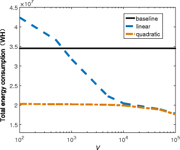
Comparison of total energy consumption under different control policies
-
2.
It is observed that the energy consumption is massive where V is small in Fig. 7. Particularly, under the linear control policy, it is even higher than baseline. We attribute it to excessively emphasizing congestion control in virtual queues, i.e., optimizing for the Lyapunov drift function Δ(Z(t)). To relieve the problem of congestion, i.e., reducing delay time, the cloud provider distributes more servers to service for users. As a consequence, more energy are consumed by servers, and waste heat increases along with increasing energy consumption. To control the server temperature falling in a safe range and guarantee the system reliability, cooling system has to efficiently work on absorbing heat. Thus, energy consumed by cooling system also increases. To the contrary, as V grows, we pay more attention to minimizing energy consumption instead of response time. Hence, the less servers, the less waste heat and energy consumption.
-
3.
The energy consumption under linear control policy is dramatically more than the one controlled by quadratic policy when V<104. In other words, the energy consumption under quadratic control policy verges on the optimum. We just approximately solve the objective function by tightening boundary. Since B L >B Q , the bound calculated by the linear algorithm is looser than the counterpart computed by the quadratic algorithm.
-
4.
The energy consumption trend under linear control policy is almost in coincidence with the curve under quadratic control policy when V>104. When V is greater than a threshold, we incline to optimize for total energy consumption. Moreover, the order of magnitude of optimizing energy significantly overcomes that of reducing delay.

To visually compare energy consumption under different control policies, we introduce the comparison table in the form of specific values (Table 1) and saving proportion (Table 2). In conclusion, the quadratic control policy is more efficient with respect to the linear control policy in terms of total energy consumption.
Component energy and PUE
The component energy is plotted in Fig. 8, which is similar with total energy consumption (Fig. 7). The number of servers have a direct effect on server energy consumption. Most of energy for CPU computing dissipates in the form of waste heat, which leads to server temperature raising up. In order to guarantee normal server operation, cooling system must work hard to maintain server temperature within a safe range. During this process, component energy and total energy are in a positive correlation, which is visually expressed in Figs. 7 and 8. In addition, as V grows, the number of active servers gradually reduces. As a result, the average server temperature and cooling temperature is building up, which is clearly illustrated in Figs. 9 and 10. Considering these performance metrics, it is clear that the quadratic control policy is more appropriate.

Energy comparison for different components under linear and quadratic control. a Server energy, b Cooling energy

The relationship between number of servers and average server temperature. a linear, b quadratic

The average temperature comparison between IT and cooling subsystem. a linear, b quadratic
Figure 11 depicts the comparison of two policies in terms of PUE. PUE is computed through dividing total energy by computing energy, which is a typical performance metric. A PUE value closed to 1, indicates a higher proportion of computing energy. P U E=1 is an ideal state, which means all energy is consumed by the useful work, i.e., CPU operation. Through Fig. 11, we find that the PUE value under the liner control policy is lower than the counterpart uner the quadratic control policy. It means that the linear control policy is superior to the quadratic control policy in terms of the metric PUE. However, as shown in Figs. 7 and 8, the quadratic control is more efficient in both the total energy and the component energy. The conclusion based on the metric PUE is opposite to the state of actual energy consumption. Hence, the metric PUE accepted by the field experts is not enough to diagnose whether a data center is efficient or not.

Power usage efficiency vs. V
Number of active servers
The control variable m j (t), i.e., the number of servers distributed to users, has a decisive influence on total energy consumption in data center. The number of servers providing service for users under linear and quadratic control policies is illustrated in Fig. 12. We use application 1 with V=1000 as an example to analyze this phenomenon. It is obvious that the number of servers under quadratic control policy is nearly always less with respect to the linear control policy. It depends on the flexibility of control variable value. It is observed that the blue line fluctuates drastically compared with the yellow line. Extensive simulations demonstrate that the similar phenomenon can also be found for other applications and a wider range of V value. The average number of active servers is depicted in Fig. 13. Holistically, as V grows, the number of active servers under linear control policy declines and almost equates to the counterpart under quadratic control policy.

Servers allocated to user1 with V=1000

Comparison in average number of active servers under different control vs.V
Average server temperature
The average server temperature fluctuation with the increasing V is displayed in Table 3. This result is attributed to the amount of workloads assigned to a server. A larger V means that more attention is paid to optimize energy consumption. As a result, fewer servers are distributed to users, and more workloads is allocated to a single server. CPU computing under high load leads to higher degree server temperature. This relationship is reflected in Fig. 9. Besides, the trend of server temperature is in correspondence with energy consumption. When V∈[100,10000], since the server energy consumption under the linear policy is higher than the counterpart under the quadratic policy, the server temperature for the linear control policy is much larger.
To guarantee server stability and reliability, we set the upper bound of server temperature as 60 °C. As shown in Fig. 14, for the linear control policy, the average server temperature exceeds the bound when V>1000. But under quadratic control policy, it doesn’t go beyond the bound until V value is closed to 5000. In terms of thermal management, the quadratic control policy is more efficient compared with the linear control policy.

The average server temperature vs. V
The probability distribution functions of server inlet temperature under linear and quadratic control policies are displayed in Figs. 15 and 16, respectively. Taking the practical operation into account, only the curves representing V=500,1000,5000,10,000 are depicted. It can be validated that server temperature rises up with increasing V in the two figures. Using 60 °C as an example, the proportion of instantaneous temperature of servers lower than 60 °C is smaller and smaller from V=500 to V=10000 (Fig. 15). Moreover, we can observe that more than half of server temperatures under the linear control policy violates “soft” server temperature constraint 60 °C. But under the quadratic control policy, it is almost all lower than 60 °C. Specifically, we list out the probability of instantaneous temperature of servers below 60 °C in Table 4. It is obvious that the quadratic control policy is superior to a linear one in guaranteeing the “soft” server temperature constraint (≤60 °C).

The probability distribution function of server instantaneous temperature under linear policy vs.V

The probability distribution function of server instantaneous temperature under quadratic policy vs.V
Conclusion
In this paper, we formulate the total energy minimization problem subject to the “soft” server temperature constraint. Based on the Lyapunov Optimization theory, we design linear and quadratic control policies to obtain the near-optimal solution. The “soft” server temperature constraint is translated into the mean rate stability of virtual queues. Furthermore, we evaluate the system performance through extensive simulations with various parameters. Substantial results indicate that the quadratic control policy is closer to the optimum, whatever in saving energy or complying with the temperature constraint. We set a weight parameter V to balance energy consumption and server temperature constraint. As a consequence, setting V around 5000 under the quadratic control policy is the optimal trade-off: the proportion of energy saving is up to 41.83%, and the “soft” server temperature constraint violation proportion is 17.7%.
Abbreviations
- CFD:
-
Computational fluid dynamics
- CoP:
-
Coefficients of performance
- CRACs:
-
Computer room air conditioners
- CUs:
-
Cloud users
- CP:
-
Cloud provider
- DVFS:
-
Dynamic voltage and frequency scaling
- HVAC:
-
Heat ventilation & air conditioner
- IT:
-
Information technology
- LO:
-
Lyapunov optimization
- PUE:
-
Power usage efficiency
- QoS:
-
Quality of service
- VM:
-
Virtual machine
References
Dayarathna M, Wen Y, Fan R (2016) Data center energy consumption modeling: a survey. IEEE Commun Surv Tutorials 18(1):732–794.
Gu L, Zeng D, Guo S, Stojmenovic I (2015) Optimal task placement with qos constraints in geo-distributed data centers using dvfs. IEEE Trans Comput 64(7):2049–2059.
Tolia N, Wang Z, Ranganathan P, Bash C, Marwah M, Zhu X (2009) Unified thermal and power management in server enclosures In: ASME 2009 Interpack Conference Collocated with the ASME 2009 Summer Heat Transfer Conference and the ASME 2009, International Conference on Energy Sustainability, Vol. 76, 721–730, San Francisco.
Gandhi A, Gupta V, Harchol-Balter M, Kozuch MA (2010) Optimality analysis of energy-performance trade-off for server farm management. Perform Eval 67(11):1–23.
Zhou X, Yang J (2010) Performance-aware thermal management via task scheduling. ACM Trans Archit Code Optim 7(1):1–31.
Li S, Wang S, Abdelzaher T, Kihl M, Robertsson A (2012) Temperature aware power allocation: an optimization framework and case studies. Sustain Comput Inform Syst 2(3):117–127.
Yeo S, Hossain MM, Huang JC, Lee H-HS (2014) ATAC: Ambient Temperature-Aware Capping for Power Efficient Datacenters In: Acm Symposium on Cloud Computing, 1–14, Seattle.
Iyengar M, Schmidt R (2009) Analytical modeling for thermodynamic characterization of data center cooling systems. J Electron Packag 131(2):9.
Cho J, Kim Y (2016) Improving energy efficiency of dedicated cooling system and its contribution towards meeting an energy-optimized data center. Appl Energy 165:967–982.
Wan J, Gui X, Zhang R, Fu L (2017) Joint cooling and server control in data centers: A cross-layer framework for holistic energy minimization. IEEE Syst J PP(99):1–12.
Mohaqeqi M, Kargahi M (2014) Temperature-aware adaptive power management: an analytical approach for joint processor and cooling. Sustain Comput Inform Syst 4(4):307–317.
Li S, Le H, et al. (2012) Joint Optimization of Computing and Cooling Energy: Analytic Model and A Machine Room Case Study In: IEEE International Conference on Distributed Computing Systems, Macau.
Zhang S, Ahuja N, Han Y, Ren H, Chen Y, Guo G (2015) Key Considerations to Implement High Ambient Data Center In: Thermal Measurement, Modeling & Management Symposium, 147–154, San Jose.
Pervila M, Kangasharju J (2010) Running Servers Around Zero Degrees In: ACM SIGCOMM Workshop on Green NETWORKING, 9–14, New Delhi.
Neely MJ (2010) Stochastic Network Optimization with Application to Communication and Queueing Systems. vol. 3. Morgan and Claypool Publishers, San Rafael.
UniCloud, Co., Ltd. http://www.uni-cloud.cn/. Accessed 2009.
Pelley S, Meisner D, et al. (2009) Understanding and Abstracting Total Data Center Power In: In Workshop on Energy-Efficient Design.
Barroso LA, Hölzle U (2007) The Case for Energy-proportional Computing In: IEEE Computer Society Press, 33–37, Washington.
Meisner D, Gold BT, Wenisch TF (2009) PowerNap: Eliminating Server Idle Power In: International Conference on Architectural Support for Programming Languages and Operating Systems, 205–216, Washington.
Duan L, Zhan D, Hohnerlein J (2015) Optimizing Cloud Data Center Energy Efficiency Via Dynamic Prediction of CPU Idle Intervals In: IEEE International Conference on Cloud Computing, 985–988, New York.
Aldhahri E (2017) Dynamic Voltage and Frequency Scaling Enhanced Task Scheduling Technology Toward Green Cloud Computing In: 2016 4th Intl Conf on Applied Computing and Information Technology/3rd Intl Conf on Computational Science/Intelligence and Applied Informatics/1st Intl Conf on Big Data, Cloud Computing, Data Science & Engineering, Las Vegas.
Kamga CM (2012) CPU Frequency Emulation Based on DVFS In: IEEE Fifth International Conference on Utility and Cloud Computing, 367–374, Chicago.
Wang S, Qian Z, Yuan J, You I (2017) A dvfs based energy-efficient tasks scheduling in a data center. IEEE Access, New York 5:13090–13102.
Takouna I, Meinel C (2015) Coordinating VMs’ Memory Demand Heterogeneity and Memory DVFS for Energy-efficient VMs Consolidation In: IEEE International Conference on Internet of Things, 478–485.
Arroba P, Moya JM, Ayala JL, Buyya R (2015) DVFS-Aware Consolidation for Energy-Efficient Clouds In: International Conference on Parallel Architecture and Compilation, San Francisco.
Zhang W, Wen Y, et al. (2016) Towards joint optimization over ict and cooling systems in data centre: A survey. IEEE Commun Surv Tutorials 18(3):1596–1616.
Arghode VK, Joshi Y (2015) Experimental investigation of air flow through a perforated tile in a raised floor data center. J Electron Packag 137(1).
Erden HS, Yildirim MT, Koz M, Khalifa HE (2017) Experimental Investigation of CRAH Bypass for Enclosed Aisle Data Centers. IEEE Trans Components Packag Manuf Technol 7(11):1795–1803.
Athavale J, Joshi Y, Yoda M, Phelps W (2016) Impact of Active Tiles on Data Center Flow and Temperature Distribution In: Thermal and Thermomechanical Phenomena in Electronic Systems, 1162–1171, Las Vegas.
Cho J, Kim Y (2015) Improving energy efficiency of dedicated cooling system and its contribution towards meeting an energy-optimized data center. Appl Energy 165:967–982.
Ham SW, Kim MH, Choi BN, Jeong JW (2015) Energy saving potential of various air-side economizers in a modular data center. Appl Energy 138(C):258–275.
Khalaj AH, Scherer T, Halgamuge SK (2016) Energy, environmental and economical saving potential of data centers with various economizers across australia. Appl Energy 183:1528–1549.
Precision Cooling for Critical Spaces. https://ctrltechnologies.wordpress.com/. Accessed 2014.
Yeo S, Hossain MM, et al. (2014) ATAC: Ambient Temperature-Aware Capping for Power Efficient Datacenters In: Acm Symposium on Cloud Computing.
Parolini L, Sinopoli B, Krogh BH, Wang Z (2011) A cyber-physical systems approach to data center modeling and control for energy efficiency. Proc IEEE 100(1):254–268.
Tang Q, Mukherjee T, Gupta SKS, Cayton P (2006) Sensor-Based Fast Thermal Evaluation Model For Energy Efficient High-Performance Datacenters In: International Conference on Intelligent Sensing and Information Processing, 203–208.
Joshi Y, Kumar P (eds)2012. Energy Efficient Thermal Management of Data Centers. Springer, New York.
Schmidt R, Vallury A, Iyengar M (2011) Energy Savings Through Hot and Cold Aisle Containment Configurations for Air Cooled Servers in Data Centers In: ASME 2011 Pacific Rim Technical Conference and Exhibition on Packaging and Integration of Electronic and Photonic Systems.
Arghode VK, Sundaralingam V, et al. (2013) Thermal characteristics of open and contained data center cold aisle. J Heat Transfer 135(6).
Tang Q, Gupta SKS, Varsamopoulos G (2008) Energy-efficient thermal-aware task scheduling for homogeneous high-performance computing data centers: A cyber-physical approach. IEEE Trans Parallel Distributed Syst 19(11):1458–1472.
Pakbaznia E, Pedram M (2009) Minimizing Data Center Cooling and Server Power Costs In: International Symposium on Low Power Electronics and Design.
Chen H, Kesavan M, et al. (2011) Spatially-aware optimization of energy consumption in consolidated data center systems. Weed Res 52(6):551–563.
96 MacBook Pro’s in one rack. https://simbimbo.wordpress.com/.
Heath T, Centeno AP, George P, and LR (2006) Temperature Emulation and Management for Server Systems In: International Conference on Architectural Support for Programming Languages and Operating Systems, 106–116.
Parolini L, Sinopoli B, Krogh BH, Wang Z (2012) A cyber–physical systems approach to data center modeling and control for energy efficiency. Proc IEEE 100(1):254–268.
Hackenberg D, Patterson MK (2016) Evaluation of a New Data Center Air-cooling Architecture: The Down-flow Plenum In: 15th IEEE Intersociety Conference on Thermal and Thermomechanical Phenomena in Electronic Systems (ITherm), Las Vegas.
Acknowledgements
The authors would like to thank anonymous reviewers for their comments to improve the quality of this paper.
Funding
This work was supported in part by the National Natural Science Foundation of China under Grant 61502255, in part by Inner Mongolia Science & Technology Plan, in part by the Inner Mongolia Provincial Natural Science Foundation under Grant 2014BS0607, and in part by the Science Research Project for Inner Mongolia Universities under Grant NJZY14064.
Availability of data and materials
Not applicable.
Author information
Authors and Affiliations
Contributions
LF designed two control algorithms, proved analytical results, and drafted the manuscript. JW provided the initial idea of this paper and analyzed results about system performance. JY built and debugged the simulator. DC wrote related works. GZ participated in the energy consumption modeling and verification. All authors read and approved the final manuscript.
Corresponding author
Ethics declarations
Competing interests
The authors declare that they have no competing interests.
Publisher’s Note
Springer Nature remains neutral with regard to jurisdictional claims in published maps and institutional affiliations.
Additional information
Authors’ information
Lijun Fu is currently working toward the M.Sc. degree in computer science at the Inner Mongolia University of Technology, Hohhot, Inner Mongolia, China. She has authored or co-authored several papers concentrating on the energy management issue in cloud data centers. Her research interests include dynamic optimization, performance analysis of distributed systems, and data mining.
Jianxiong Wan received the Ph.D. degree in computer science from the University of Science and Technology Beijing, Beijing, China, in 2013. He was a Post-Doctoral Research Fellow with Massey University, Palmerston North, New Zealand (2016−2017), and a Visiting Researcher with Nara Institute of Science and Technology (NAIST), Japan (2017-2018). His research interests include dynamic optimization and performance analysis of distributed systems and avionics systems with a special focuses on the cloud and wireless networks.
Jie Yang received his Master’s Degree in Management Science from Beijing Information Science and Technology University (BISTU) and currently is a consulting engineer in Beijing BeiZi Information Engineering Consulting Co., Ltd. His research interest is large scale system integration.
Dongdong Cao obtained Master’s Degree in Communication Engineering from Xi ’an institute of communications, Xi’an, China. He is an engineer in Xi’an Satellite Tracking, Telemetering and Control Center with research interests concentrating on networking technologies and cloud computing, etc.
Gefei Zhang received the M.Sc. degree in computer science from the Inner Mongolia University of Technology, Hohhot, Inner Mongolia, China. She joined Inner Mongolia Agricultural University in 2017. She is interested in dynamic optimization and performance analysis of distributed systems.
Rights and permissions
Open Access This article is distributed under the terms of the Creative Commons Attribution 4.0 International License(http://creativecommons.org/licenses/by/4.0/), which permits unrestricted use, distribution, and reproduction in any medium, provided you give appropriate credit to the original author(s) and the source, provide a link to the Creative Commons license, and indicate if changes were made.
About this article

Cite this article
Fu, L., Wan, J., Yang, J. et al. Dynamic thermal and IT resource management strategies for data center energy minimization. J Cloud Comp 6, 25 (2017). https://doi.org/10.1186/s13677-017-0094-z
Received:
Accepted:
Published:
DOI: https://doi.org/10.1186/s13677-017-0094-z