
Abstract
In this paper, we study the performance of asynchronous and nonlinear FBMC-based multi-cellular networks. The considered system includes a reference mobile perfectly synchronized with its reference base station (BS) and K interfering BSs. Both synchronization errors and high-power amplifier (HPA) distortions will be considered and a theoretical analysis of the interference signal will be conducted. On the basis of this analysis, we will derive an accurate expression of signal-to-noise-plus-interference ratio (SINR) and bit error rate (BER) in the presence of a frequency-selective channel. In order to reduce the computational complexity of the BER expression, we applied an interesting lemma based on the moment generating function of the interference power. Finally, the proposed model is evaluated through computer simulations which show a high sensitivity of the asynchronous FBMC-based multi-cellular network to HPA nonlinear distortions.
1 Introduction
Multicarrier modulations can be separated into two main classes: cyclic prefix-based orthogonal frequency division multiplexing (CP-OFDM) and filter bank-based multicarrier (FBMC). The first class is the most widely used since it has been adopted by many major communication standards, e.g., DAB, DVB-T, IEEE802.11a/g (Wi-Fi), IEEE 802.16 (WiMAX), and LTE. However, OFDM systems still have some drawbacks such as the high side lobes of the rectangular pulse shape (transmission/reception filter) and a loss of the spectral efficiency due to the cyclic prefix extension. Because of the aforementioned weaknesses, researchers are more and more interested by FBMC modulations which employ a frequency well-localized FIR filter with small side lobes instead of the rectangular pulse shape used in OFDM. This makes FBMC systems more spectral efficient and less sensitive to frequency errors compared to OFDM [1].
When a multicarrier modulation (OFDM or FBMC) is employed, the performance of multi-cellular networks depends extensively on how well the orthogonality among subcarriers is maintained at the receiver. In an asynchronous system, this orthogonality is destroyed due to synchronization errors which include timing offsets and carrier frequency/phase offsets. The problem of asynchronism in multicarrier systems has been intensively investigated in the literature for OFDM as well as for FBMC systems [2–8]. The sensitivity of OFDM/FBMC systems to synchronization errors has been illustrated in terms of signal-to-interference ratio (SIR) in [1, 3, 7] and in terms of bit error rate (BER) in [8, 9], by exploiting the Gaussian approximation of the intercarrier interference. An interesting work in relationship with the scope of this paper is [2] (resp. [5]) where the authors have presented a theoretical analysis of the average error rate of an asynchronous OFDM (resp. FBMC)-based multi-cellular network in the special case of interleaved (resp. block) subcarrier assignment scheme. More recently, Medjahdi et al. [6] have presented an interference modeling based on the so called interference tables [4] for asynchronous OFDM and FBMC systems. This model and the results of [5] will be very useful to accomplish the developments of this paper.
Another serious issue with OFDM and FBMC systems is the fact that the transmitted signal is a sum of a large number of independently modulated subcarriers. Thus, they suffer from high peak-to-average power ratio (PAPR) which makes the system very sensitive to nonlinear distortion (NLD) caused by nonlinear devices such as high-power amplifiers (HPA). This problem has been largely studied for OFDM systems. The impact of NLD on OFDM signals was presented in [10, 11] and a performance analysis of nonlinear OFDM and OFDM-MIMO systems was derived in [12, 13]. As for FBMC systems, the authors in [14] carried out a theoretical analysis of BER performance for nonlinearly amplified FBMC/OQAM signals under additive white Gaussian noise (AWGN) and Rayleigh fading channels. Similarly, [15] has recently derived a closed-form expression for the BER of gray-coded M-ary (QAM or OQAM)-based OFDM in the presence of HPA NLD under a frequency flat fading Rayleigh channel.
It is worth noting that there are limited studies that investigate the problem of the joint effect of non-synchronization and HPA nonlinearities on multicarrier systems. An interesting one is [16], where the authors evaluated the BER of multicarrier DS-CDMA downlink systems subject to these impairments in frequency-selective Rayleigh fading channels, assuming QAM modulation. In this paper, we study the joint effect of synchronization errors and HPA nonlinear distortions on FBMC-based multi-cellular networks. We will derive exact expressions of average error rates for the considered system by carrying out an analytical interference analysis in frequency-selective fading channels. It is worth noting that there are limited studies that investigate the problem of joint effects of non-synchronization and HPA nonlinearities on multicarrier systems. An interesting one is [17], where the authors analyzed the interference caused by nonlinear power amplifiers together with timing errors on multicarrier OFDM/FBMC transmissions. In this work, we will consider both frequency and timing errors in addition to HPA NLD and we will plot BER curves as functions of SNR for different frequency offset (CFO) ranges and different levels of the nonlinear noise power. Regarding FBMC modulation, a cosine modulated multitone (CMT) system will be considered and the results can be easily extended to staggered modulated multitone (SMT) systems since a CMT signal can be obtained from a SMT one through a simple modulation step [18].
The remainder of this paper is organized as follows. In Section 2, the considered CMT-based multi-cellular network is introduced and the joint effect of HPA NLD and synchronization errors is described. In Section 3, we present the analytical interference analysis. The BER analysis is carried out in Section 4. Section 5 includes the evaluation of the obtained BER expressions through simulation results. Finally, Section 6 concludes this paper.
2 System model
We consider the downlink transmission scenario of the CMT-based multi-cellular network depicted in Fig. 1. MU 0 is the reference mobile user who communicates with the reference base station BS 0. The other base stations BS k ,k=1…6 represent an interfering source for MU 0. In a regular hexagonal cellular system (hexagonal coordinates system), where the reference BS is located at the origin (0,0), the reference mobile at the coordinates point (u 0,v 0) and the kth interfering BS at (u k ,v k ), then the distance between the reference mobile and the kth base station is given by ([19], pp. 140)

CMT-based multi-cellular network
where R is the cell radius.
The transmitted signal from the kth base station to the reference mobile is a CMT signal given by [18]
where
-
T is the CMT symbol duration and g(t) is the prototype filter impulse response,
-
\(s_{n}^{m,k}\) is the transmitted pulse-amplitude modulated (PAM) symbol by the kth base station, at the mth subcarrier on the nth time index,
-
\(\gamma _{m,n}(t)=g(t-nT)e^{j\frac {\pi }{2T} t}e^{j\Phi ^{m}(t)}\) and \(\Phi ^{m}(t)=m(\frac {\pi }{T} t+ \frac {\pi }{2})\),
-
F k is the set of subcarriers that are assigned to the kth base station. In this paper, we will consider the block subcarrier assignment, described in Fig. 2, for frequency reuse scheme.
Fig. 2 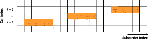
Block subcarrier assignment

Concerning the channel model, we will consider a common model for interference analysis in microcellular mobile systems, in which the useful signal received from the reference BS is assumed to experience Nakagami−m fading, whereas all the interfering signals from the neighboring BSs experience Rayleigh fading [2]. The impulse response of the multipath channel between the kth base station and the reference mobile is
where τ 0<τ 1<…τ L−1<τ max and τ max is the maximum delay spread of the channel, and {h k,l ,∀k,l} are the complex path gains which are assumed mutually independent, where \(E\left [ h_{k,i}, h_{k,i}^{*} \right ]=\gamma _{k,i}\) and \(E\left [ h_{k,i}, h_{k,j}^{*} \right ]=0\), if i≠j. We further assume that the power is normalized such that \(\sum _{l=0}^{L-1} \gamma _{k,l}=1, \forall k\).
We assume a perfect synchronization between MU 0 and BS 0. However, MU 0 is not necessarily synchronized with the other base stations. In addition, we consider the presence of HPA nonlinear distortions. These distortions can be modeled using the Bussgang theorem which states that for a Gaussian signal x(t) which undergoes a nonlinear distortion and produce an output signal y(t), the cross-correlation function R xy (τ) is related to the auto-correlation function R xx (τ) by the following expression
where \(\phantom {\dot {i}\!}\alpha =|\alpha | e^{\phi _{\alpha }}\) is a complex factor.
An interesting result from the Bussgang theorem is that the output y(t) can be written as [10]
where η(t) is a zero mean additive noise, uncorrelated to x(t) and with variance \(\sigma _{\eta }^{2}=E\left [ \left |\eta \right |^{2} \right ]\).
On the other hand, the received signal from the kth interfering base station BS k is affected by a timing offset τ k , a carrier frequency offset ε k , and a phase offset ϕ k . Therefore, we can express the composite signal at the reference receiver by the sum of the desired signal coming from BS 0 and the interference signal coming from the surrounding base stations BS k ,k=1…K
where
-
* is the convolution operator,
-
K is the total number of neighboring cells,
-
x k is the interference signal transmitted by the base station BS k ,
-
n(t) is the additive white Gaussian noise (AWGN) with two-sided power spectral density N 0/2,
-
β is the path loss exponent.
3 Interference analysis
3.1 Interference analysis in an AWGN channel
In this subsection, we will derive the interference power expression of the considered CMT-based multi-cellular network in the case of AWGN channels. To this end, let us consider the transmission of an individual PAM symbol \({s_{n}^{m}}\) from an interfering cell on its mth subcarrier (in the nth time index) to the reference mobile in the presence of all the sources of distortion presented in the last section (i.e., synchronization errors and NLD). The received signal will be then expressed as follows:
We recall that \(\Phi ^{m}(t)=m(\frac {\pi }{T} t+ \frac {\pi }{2})\).
After demodulation, the interference signal received on the 0th subcarrier and the 0th time index (for simplicity’s sake) of the reference mobile output can be given by the following expression
where \(\hat {\eta }_{0}^{0}\) and \(\hat {n}_{0}^{0}\) are given by
Therefore, we can express the power of the interference as follows
where ψ=(τ,ε,θ), θ=ϕ+ϕ α and E s is the PAM symbol energy.
The interference power \( \mathcal {I}(\psi,m)\) can be explicitly expressed if we take into account some observations. First, we refer to the PHYDYAS prototype filter designed by Bellanger using the frequency sampling technique [20]. Furthermore, we assume that the timing error τ is small enough such that the prototype filter impulse response g(t) can be considered constant between t and t−τ, i.e., g(t−τ)≈g(t). Using the above observations and the results of [5], the expression of the interference power becomes
where we have considered (for simplicity’s sake) that the interference signal is coming from the 0th time index symbol.
In Eq. (11), J(ψ,m) is the integral given by the following expression
For a PHYDYAS prototype filter with an overlapping factor κ=4 and frequency coefficients G 0=1/2, G 1=0.971960, \(G_{2}=\sqrt {2}/2\), and G 3=0.235147 [5, 20], the expression of the integral J(ψ,m) will become
where \(\Theta _{m}= \theta +(1-\frac {2\tau }{T})\frac {\pi }{2}m\).
After a few steps of straightforward manipulations, one finds that
where \(\Gamma _{0}(\psi,m,t)=\frac {\sin {\left (\left (\frac {\pi }{T}m+2\pi \varepsilon \right) t +\Theta _{m} \right)} }{\frac {\pi }{T}m+2\pi \varepsilon }\) and
Similarly, \({\Gamma _{2}^{q}}(\psi,m,t)\) and \(\Gamma _{3}^{q,q'}(\psi,m,t)\) are, respectively, the primitives of integrals shown in the third and fourth terms of Eq. (13).
By putting
we can rewrite the interference power \(\mathcal {I}(\psi,m)\) as follows:
with \(\chi (\psi,m)=\left | \left.\Gamma (\psi,m,t) \right |_{0}^{4T} \right |^{2}\).
3.2 Interference power in a frequency-selective channel and SINR expression
According to [5], the interference power arriving through a frequency-selective channel, in the multi-cell model described in Section 2, can be calculated using the following expression:
where
-
\(\mathcal {I}(\psi _{k},m,\alpha _{k})\) (Eq. (17)) is the power of the interference caused by the kth base station on the mth subcarrier and corresponding to an error vector ψ k =(τ k ,ε k ,θ k ),
-
|H k (m)|2 is the power channel gain between the kth interfering base station and the reference receiver.
Similarly, we can express the power of the total nonlinear noise signal coming from all the K interfering base stations as follows:
where \(\sigma _{\hat {\eta }_{0,k}^{0}}^{2}(\varepsilon _{k})=E\left [ \left | \hat {\eta }_{0,k}^{0}(\varepsilon _{k}) \right |^{2} \right ]\) is the variance of the received nonlinear noise \(\hat {\eta }_{0,k}^{0}(\varepsilon _{k}) \).
Concerning the power of the desired signal, which is assumed to be perfectly synchronized with the reference base station, it can be simply expressed as
Using the following expression of the signal to interference plus noise ratio
And by substituting Eqs. (18), (19), and (20) in Eq. (21), the SINR expression can be rewritten as follows:
where B sc is the bandwidth of 0th subchannel.
In order to get a more explicit expression of the SINR, we suggest in the following subsection to analyze the expression of the received nonlinear noise variance \(\sigma _{\hat {\eta }_{0,k}^{0}}^{2}(\varepsilon _{k})\).
3.3 Variance of the received nonlinear noise
In this subsection, we will simplify the expression of the received nonlinear noise \(\hat {\eta }\) in order to find a closed-form expression of its variance \(\sigma _{\hat {\eta }}^{2}\). We note that the BS index will be omitted in this subsection for simplicity’s sake.
Recall that the received nonlinear noise is expressed by
We consider PHYDYAS prototype filter whose impulse response is given by [20]
where κ is the overlapping factor and G q ,q=0,…,κ−1 are the frequency coefficients of the filter.
Furthermore, the nonlinear noise η(t) can be expressed as the sum of his real and imaginary components : η(t)=η r (t)+j η i (t).
Therefore, the received nonlinear noise \(\hat {\eta }_{0}^{0}\) can be rewritten as
After a few steps of straightforward manipulations and by considering the following observations : (i) η r (t)=η i (t)=η r is constant in the interval [0,κ T], (ii) the overlapping factor κ=4, one can find that
Therefore, the variance \(\sigma _{\hat {\eta _{k}}}^{2}\) of the received nonlinear noise from the kth interfering BS can be expressed as
where \(a(\varepsilon _{k})=8 \frac {T^{2}}{\pi ^{2}} c^{2}(\varepsilon _{k}) (4T\varepsilon _{k}+1)^{2} \sin ^{2}(4\pi T\varepsilon _{k}) \left [1-\sin (8\pi T\varepsilon _{k})\right ]\) and \(c(\varepsilon _{k})=2\sum _{q=0}^{3} (-1)^{q} \frac {G_{q}}{q^{2}-(4T\varepsilon _{k} +1)^{2}}\).
Then, the SINR expression will become as follows:
where \(\text {SNR}_{\eta _{k}}=E_{s}/\sigma _{\eta _{k}}^{2}\) and \(b=\frac {1}{d_{0}^{-\beta } SNR} =\frac {N_{0} B_{sc}}{d_{0}^{-\beta } E_{s}}\).
To get a more simplified SINR expression, we introduce the following new variables
and
Finally, we obtain the following final SINR expression:
4 Bit error rate expression
We know that the BER of 4-PAM modulation in AWGN channels, when the decision variables are “pure” Gaussian RVs, is given by the following expression [21]:
where erfc denotes the complementary error function given by
and is SNR the signal to noise ratio.
In our analysis, we can obtain the conditional BER in the presence of interference by conditioning on the set of random variables \(\mathcal {H}=\left \{ H_{0}, H_{k}(m), \forall k,m \right \}\), as shown by the following equation:
Our objective is to derive the average BER which can be obtained by averaging out the vector of random variables \(\mathcal {H}\) from Eq. (32). Unfortunately, this average can not be calculated directly because we do not have a closed-form expression for the probability density function (pdf) of the SINR. In order to get the BER average with a reduced computational complexity, we refer to the following lemma [2] and we propose to use the results of [5].
Lemma 1
Let x be a unit-mean gamma random variable with parameter λ=1 and a pdf f(x)=e −x,x≥0, and let y be an arbitrary non-negative random variable that is independent of x. Then
where \(\mathcal {M}_{y}(z)=E_{y}\left [ e^{-zy} \right ]\) is the moment generating function (MGF) of y.
By using this lemma and the results of [5], we can express the final expression of the average BER for the considered asynchronous and nonlinear FBMC-based multi-cellular network as follows:
where
-
|A| stands for the determinant of the matrix A,
-
\(\Omega _{k}=\left [\rho _{i,j}\right ]_{(i,j)\in F_{k}\times F_{k}}\) is the correlation matrix of the random variables {|H k (m)|2,m∈F k },
-
L k denotes the number of subcarriers allocated to the kth BS and \(I_{L_{k}}\) is the L k ×L k identity matrix,
-
\(D_{k}^{\chi _{d}}\) is a diagonal matrix with diagonal elements \(D_{k}^{\chi _{d}}(i,i)=\chi _{d}(\psi _{k},i)\), i∈F k .
Equation (34) shows clearly that, in addition to the interference caused by synchronization errors, the BER performance of the studied system is affected by HPA nonlinearities and especially by the nonlinear noise η. A detailed analysis of this expression will be carried out in the next section via computer simulations.
5 Simulations
In this section, we present numerical results for the analytical BER expression that we have derived in the previous section for the considered CMT based multi-cellular network. The obtained BER expression will be evaluated using different evaluation parameters such as the signal to nonlinear noise ratio, the frequency error range, and the input back-off of the power amplifier. We consider the six neighboring cells surrounding the reference mobile user as interfering base stations. The cell radius is R=1 km and the path loss exponent β is equal to 3.76. Furthermore, we consider a CMT system with N=64 subcarriers transmitting 4-PAM modulated symbols. PHYDYAS prototype filter is used with overlapping factor κ=4. The PHYDYAS prototype filter is obtained using the frequency sampling technique described in [20]. The simulation curves are obtained using a solid state power amplifier (SSPA) model with AM/AM distortion given by the following expression:
A 0 is the HPA input saturation level, υ is the small signal gain, and p is a parameter that controls the smoothness of the transition from the linear region to the saturation region.
Regarding the frequency specifications, they match those of the IEEE 802.11 a/g standards, i.e., a bandwidth of 2 MHz, a subcarrier spacing of 0.3125 MHz and a symbol duration of T=1.6 μs. We recall that the fractional normalized CFO ε N =2T ε is defined in the range −0.5≤ε N ≤0.5, which means that the CFO ε takes values between −0.16 and 0.16. In the curves presented in this section, ε will be taken in the range [0,0.16] (unless otherwise stated). A numerical computing environment (MATLAB) is used to simulate the interference CMT signals coming from the six interfering base stations. A 4-PAM CMT receiver is also simulated and the BER is directly computed by comparing the decoded symbols with the real transmitted symbols from the reference base station. Finally, for the Rayleigh fading channel model, we have considered the pedestrian-A model with relative delays [0 110 190 410] ns and corresponding average powers [0 –9.7 –19.2 –22.8] dB [23].
In Fig. 3, we plot the BER of the system as a function of the SNR using expression (34) (proposed model) and the expression obtained using the derivations of Medjahdi et al. [5] (which ignores HPA effects). The perfectly synchronized scenario without HPA nonlinear distortions is also considered for comparison purposes. Figure 3 evaluates also the accuracy of the theoretical results and compares it with the simulation results. In order to observe the evolution of the BER performance for different nonlinear distortion levels, the BER curves of Fig. 3 are plotted for various values of the signal to nonlinear noise ratio (SNR η =6,12, and 18 dB). As shown in Fig. 3, synchronization errors cause a severe degradation in the BER. This is found in agreement with the results of [5] where no HPA NLD effect is considered. Moreover, when the signals coming from the different interfering base stations are affected by a HPA nonlinearity as illustrated by the proposed model (Eq. (34)), the BER degradation is more significant. Example: to achieve a BER of 1.3×10⁻², the asynchronous nonlinear system requires a value of SNR equal to 24 dB (When SNR η =12 dB) while the asynchronous system without HPA nonlinearities requires only 19 dB of SNR, which means a loss of 5 dB in the transmitted signal power for the former. Another important observation from Fig. 3 is that the BER performance depends strongly on the signal to nonlinear noise ratio SNR η . As this parameter decreases, the gap between the BER curves corresponding to the linear system and nonlinear ones becomes significant.

CMT average BER against the SNR for different values of signal to nonlinear noise ratio SNR η =6,12,18 dB
An important parameter that defines the amount of nonlinearity introduced by a HPA is the input back-off (IBO). A high IBO value means that the power amplifier operates close to its linear region, and therefore, it introduces less nonlinear distortions. Figure 4 shows the BER plots for two values of the IBO, IBO=4 dB and IBO=8 dB. From this figure, we can see that BER performance depends heavily on the HPA IBO, which is an expected result since there is a proportionality between the nonlinear noise variance and IBO as it was stated in [14].

The average BER for two input back-off values IBO=4,8 dB
In Fig. 5, we plot the average BER curves for three different frequency offset ranges. In the first range ε∈[0.02,0.06] (scenario a), in the second range ε∈[0.06,0.1] (scenario b), and in the third range ε∈[0.1,0.14] (scenario c). The perfectly synchronized (PS) scenario is also considered for comparison purposes. The results illustrated by Fig. 5 show that the BER degradation is also related to frequency errors and becomes more significant for high values of the carrier frequency offset. For example, to achieve a BER value of 2×10⁻², the required SNR in the PS scenario is SNR=16 dB and in the asynchronous scenarios (b), (c), and (d) the required SNR is respectively equal to 18, 21, and 27 dB. These results show the high sensitivity of nonlinear CMT systems to carrier frequency offset and allow us to conclude by considering also the results of Figs. 3 and 4 that synchronization errors combined with nonlinear distortions cause a severe degradation in the performance of CMT based multi-cellular networks and a joint compensation of these two sources of distortion should be considered. Finally, we can see from the presented figures that the theoretical results show an excellent match to the corresponding simulation results despite an error floor at high SNR values (expected in interference limited scenarios).

The average BER for different CFO ranges. a PS scenario. b ε∈[0.02,0.06]. c ε∈[0.06,0.1]. d ε∈[0.1,0.14], the signal to nonlinear noise ratio is SNR η =8 dB
6 Conclusions
In this paper, we have studied jointly the effect of synchronization errors and HPA nonlinear distortions on asynchronous downlink CMT based multi-cellular networks. A scenario consisting on one reference mobile perfectly synchronized with its reference BS and K interfering BSs was considered and an exact BER expression was derived by carrying out an analytical interference analysis in the presence of a frequency-selective channel. In order to obtain explicit and less complex BER expressions, an interesting lemma based on the moment generating function of the interference power was applied. The obtained theoretical BER expression has been evaluated through simulation results using different evaluation parameters such as the signal to nonlinear noise ratio, the frequency error range, and the input back-off of the power amplifier. We found a perfect match between the simulation and the developed theoretical results. Furthermore, we have highlighted the significant performance degradation caused by the joint effect of HPA nonlinear distortions and synchronization errors.
References
H Saeedi-Sourck, Y Wu, JWM Bergmans, S Sadri, B Farhang-Boroujeny, Sensitivity analysis of offset {QAM} multicarrier systems to residual carrier frequency and timing offsets. Signal Process.91(7), 1604–1612 (2011).
KA Hamdi, YM Shobowale, Interference analysis in downlink ofdm considering imperfect intercell synchronization. Veh. Technol. IEEE Trans.58(7), 3283–3291 (2009). doi:10.1109/TVT.2009.2013959.
K Raghunath, A Chockalingam, Sir analysis and interference cancellation in uplink ofdma with large carrier frequency/timing offsets. Wireless Commun. IEEE Trans.8(5), 2202–2208 (2009). doi:10.1109/TWC.2009.071383.
Y Medjahdi, M Terre, D Le Ruyet, D Roviras, JA Nossek, L Baltar, in Signal Processing Advances in Wireless Communications, 2009. SPAWC ’09. IEEE 10th Workshop On. Inter-cell interference analysis for ofdm/fbmc systems (IEEEPerugia, 2009), pp. 598–602. doi:10.1109/SPAWC.2009.5161855.
Y Medjahdi, M Terre, D Le Ruyet, D Roviras, A Dziri, Performance analysis in the downlink of asynchronous ofdm/fbmc based multi-cellular networks. Wireless Commun. IEEE Trans. 10(8), 2630–2639 (2011). doi:10.1109/TWC.2011.061311.101112.
Y Medjahdi, Terre, Ḿ, DL Ruyet, D Roviras, Interference tables: a useful model for interference analysis in asynchronous multicarrier transmission. EURASIP J. Adv. Signal Process.2014(1), 1–17 (2014). doi:10.1186/1687-6180-2014-54.
SK Hashemizadeh, MJ Omidi, H Saeedi-Sourck, B Farhang-Boroujeny, Sensitivity analysis of ofdma and sc-fdma uplink systems to carrier frequency offset. Wirel. Pers. Commun.80(4), 1381–1404 (2014). doi:10.1007/s11277-014-2089-0.
B Aziz, F Elbahhar, in Communications (ICC), 2015 IEEE International Conference On. Impact of frequency synchronization errors on ber performance of mb-ofdm uwb in nakagami channels (IEEELondon, 2015), pp. 2698–2703. doi:10.1109/ICC.2015.7248733.
L Rugini, P Banelli, Ber of ofdm systems impaired by carrier frequency offset in multipath fading channels. IEEE Trans. Wirel. Commun.4(5), 2279–2288 (2005). doi:10.1109/TWC.2005.853884.
D Dardari, V Tralli, A Vaccari, A theoretical characterization of nonlinear distortion effects in ofdm systems. IEEE Trans. Commun.48(10), 1755–1764 (2000). doi:10.1109/26.871400.
T Araujo, R Dinis, On the accuracy of the gaussian approximation for the evaluation of nonlinear effects in ofdm signals. Comm. IEEE Trans.60(2), 346–351 (2012). doi:10.1109/TCOMM.2011.102011.110151.
L Yiming, M O’Droma, J Ye, A practical analysis of performance optimization in ostbc based nonlinear mimo-ofdm systems. IEEE Trans. Commun.62(3), 930–938 (2014). doi:10.1109/TCOMM.2014.010414.130533.
L Yiming, M O’Droma, A novel decomposition analysis of nonlinear distortion in ofdm transmitter systems. IEEE Trans. Signal Process.63(19), 5264–5273 (2015). doi:10.1109/TSP.2015.2451109.
H Bouhadda, et al., Theoretical analysis of ber performance of nonlinearly amplified fbmc/oqam and ofdm signals. EURASIP J. Adv. Sig. Proc. 2014(1) (2014). doi:10.1186/1687-6180-2014-60.
R Zayani, H Shaiek, D Roviras, Y Medjahdi, Closed-form ber expression for (qam or oqam)-based ofdm system with hpa nonlinearity over rayleigh fading channel. Wirel. Commun. Lett. IEEE. 4(1), 38–41 (2015). doi:10.1109/LWC.2014.2365023.
L Rugini, P Banelli, Joint impact of frequency synchronization errors and intermodulation distortion on the performance of multicarrier ds-cdma systems. EURASIP J. Adv. Signal Process.2005(5), 1–13 (2005). doi:10.1155/ASP.2005.730.
M Khodjet-Kesba, C Saber, D Roviras, Y Medjahdi, in Vehicular Technology Conference (VTC) Spring, 2011 IEEE. Multicarrier interference evaluation with jointly non-linear amplification and timing errors (IEEEBudapest, 2011), pp. 1–5. doi:10.1109/VETECS.2011.5956177.
B Farhang-Boroujeny, GCH Yuen, Cosine modulated and offset qam filter bank multicarrier techniques: a continuous-time prospect. EURASIP J. Appl. Sig. Pro.ID 165654:, 16 (2010).
PM Shankar, Introduction to Wireless Systems, 1st edn (Wiley, New York, 2001).
MG Bellanger, in Proceedings. ICASSP ’01, 4. Specification and design of a prototype filter for filter bank based multicarrier transmission (IEEESalt Lake City, 2001), pp. 2417–24204. doi:10.1109/ICASSP.2001.940488.
JG Proakis, Digital Communications, 4th edn (McGrawHill, NY, 2001).
KA Hamdi, A useful technique for interference analysis in nakagami fading. Commun. IEEE Trans.55(6), 1120–1124 (2007). doi:10.1109/TCOMM.2007.898823.
R ITU-R.M.1225, Guidelines for evaluation of radio transmission technologies for imt-2000, Technical report, ITU (1997). https://www.itu.int/dms_pubrec/itu-r/rec/m/R-REC-M.1225-0-199702-I!!PDF-E.pdf.
Acknowledgements
The authors would like to thank the associate editor Luca Rugini and the anonymous reviewers for valuable comments and suggestions that have led to improvements in this paper.
Funding
No funding information.
Authors’ contributions
All the authors have contributed to the study conception and design, acquisition of data, analysis and interpretation of data, drafting of manuscript, and critical revision. All authors read and approved the final manuscript.
Competing interests
The authors declare that they have no competing interests.
Author information
Authors and Affiliations
Corresponding author
Rights and permissions
Open Access This article is distributed under the terms of the Creative Commons Attribution 4.0 International License (http://creativecommons.org/licenses/by/4.0/), which permits unrestricted use, distribution, and reproduction in any medium, provided you give appropriate credit to the original author(s) and the source, provide a link to the Creative Commons license, and indicate if changes were made.
About this article

Cite this article
Elmaroud, B., Faqihi, A. & Aboutajdine, D. Sensitivity analysis of FBMC-based multi-cellular networks to synchronization errors and HPA nonlinearities. EURASIP J. Adv. Signal Process. 2017, 3 (2017). https://doi.org/10.1186/s13634-016-0441-0
Received:
Accepted:
Published:
DOI: https://doi.org/10.1186/s13634-016-0441-0