
Abstract
The current researches mainly adopt “Guide to the expression of uncertainty in measurement (GUM)” to calculate the profile error. However, GUM can only be applied in the linear models. The standard GUM is not appropriate to calculate the uncertainty of profile error because the mathematical model of profile error is strongly non-linear. An improved second-order GUM method (GUMM) is proposed to calculate the uncertainty. At the same time, the uncertainties in different coordinate axes directions are calculated as the measuring points uncertainties. In addition, the correlations between variables could not be ignored while calculating the uncertainty. A k-factor conversion method is proposed to calculate the converge factor due to the unknown and asymmetrical distribution of the output quantity. Subsequently, the adaptive Monte Carlo method (AMCM) is used to evaluate whether the second-order GUMM is better. Two practical examples are listed and the conclusion is drawn by comparing and discussing the second-order GUMM and AMCM. The results show that the difference between the improved second-order GUM and the AMCM is smaller than the difference between the standard GUM and the AMCM. The improved second-order GUMM is more precise in consideration of the nonlinear mathematical model of profile error.
1 Introduction
Profile error is an important feature to evaluate the machining quality of sculptured surfaces. More and more studies have been done to improve the algorithms of calculating the profile error [1]. The least squares fitting was adopted to evaluate the profile error of the ellipse. The data was obtained by the coordinate measuring machine (CMM) [2]. Geometry optimization approximation algorithm was proposed to calculate the elliptical profile error considering the geometric characteristics [3]. Profile error could be obtained by non-uniform rational B-splines (NURBS) surface fitting according to the data points. NURBS surface fitting was accepted when the center axis was difficult to obtain [4]. The singular value decomposition-iterative closest point method was proposed to match the measurement points and the ideal section curve. Based on this, the profile error of the blade surface was calculated and balanced [5]. Surface reconstruction was implemented by the genetic algorithm. The profile error was evaluated by calculating the shortest distance between measurement points and sculptured surface in the split spherical approximation method [6]. In our lab, Lang et al. [7] proposed the sequential quadratic programming (SQP) algorithm to calculate the profile error. The computing speed is faster, and the result is more approach to the optimal solution.
However, the method of calculating the profile error could not get the corresponding uncertainty. The “Guide to the expression of uncertainty in measurement” is a standard of evaluating the uncertainty. The international organization revised the GUM in 2008, which has been accepted all over the world [8]. GUMM is a method to estimate the uncertainty by calculating the first-order Taylor series expansion of profile error. The GUMM was used to analyze the uncertainty about the location of a hole [9]. Though the GUMM is a standard method to calculate the uncertainty, it also has some limitations. GUMM can only be applied in the linear models [10]. When the actual situation does not meet the requirement, some alternative methods are put forward. The idea of the random-fuzzy and fuzzy-random uncertainties was proposed to estimate the uncertainty [11]. GUM S1 [12] used the Monte Carlo method (MCM) to analyze the uncertainty without considering the distribution of the output variable and the format of the mathematical model. The MCM is mainly based on the statistical analysis to calculate the uncertainty [13]. When the partial derivatives of the model could not be calculated, Cox and Siebert [14] adopted the MCM to calculate the expanded uncertainty. The MCM was used to evaluate the uncertainty in an experimental model, which reduced the work load of calculating the partial derivatives in a non-linear model [15]. The proper number of the experiment is difficult to determine in the Monte Carlo simulation. The AMCM was proposed because it could adaptively select the proper number of the experiment [16]. However, the prior information of the distributions is often unknown or inaccurate in AMCM. In this situation, AMCM is not suitable to calculate the uncertainty. It can still be used as a suitable method to evaluate the GUMM. The second-order GUMM was proposed to estimate the uncertainty considering the difficulty of the prior information. In 2011, the second-order and third-order Taylor series expansion in GUMM were adopted to calculate the uncertainty in a simple non-linear model [17]. However, the relativity of variables was neglected, which led to the imprecise result. In 2013, Wen et al. [18] calculated the uncertainty of cylindricity errors in AMCM and GUMM. The model is non-linear, so the first-order Taylor series expansion is inadequate. The uncertainty of measuring points in different coordinate axes directions was not calculated, and on the contrary the measuring points uncertainty was estimated by considering the limited factors, which was imprecise and complex. Although virtual coordinate measuring machine has been developed to estimate the uncertainty [19], virtual CMM is usually adopted when the actual data is difficult to be obtained.
The paper structure is as follows: Section 2 establishes a mathematical model of profile error. In Section 3, the second-order Taylor series expansion of GUMM is proposed to calculate the uncertainty. Some improvements of GUMM are also listed. Subsequently, two practical examples are presented in Section 4. Section 5 compares and discusses the AMCM and GUMM. AMCM is used for evaluating the GUMM. The conclusion is drawn in Section 6.
2 Mathematical Model of Profile Error
Profile error is the greatest deviation between the actual sculptured surfaces and the theoretical sculptured surfaces [20], as shown in Figure 1, where t is the diameter of the enveloping spheres.

Sketch of the profile error
The model of sculptured surfaces profile error is shown as follows [7]:
where \(\alpha ,\beta ,\gamma\) are the rotation angles of measuring points along the directions of \(X\) axis, \(Y\) axis and \(Z\) axis respectively, \(\Delta x,\Delta y,\Delta z\) are the offsets along the directions of \(X\) axis, \(Y\) axis and \(Z\) axis respectively, \(s_{i} (x_{i} ,y_{i} ,z_{i} )\) is the initial measuring point, \(s_{i}^{\prime } (x_{i}^{\prime } ,y_{i}^{\prime } ,z_{i}^{\prime } )\) is the closest point. The meaning of the symbols \(\alpha ,\beta ,\gamma ,\Delta x,\Delta y,\Delta z\) is shown in Figure 2.

The meaning of the symbols
3 Uncertainty Calculation Methods
3.1 Gumm
Taylor expansion of the non-linear model \(f = f(m_{ 1} ,m_{ 2} , \ldots ,m_{n} )\) in the neighborhood of the point \((m_{ 1}^{ 0} ,m_{ 2}^{ 0} , \cdot \cdot \cdot ,m_{n}^{ 0} )\) is given as follows:
where partial derivative \(\partial f/\partial ( \cdot )\) is the sensitivity coefficient of each variable, \(\delta^{p} m_{i}\) is defined as \(\delta^{p} m_{i} { = }(m_{i} - m_{i}^{0} )^{p} ,i = 1, \ldots ,n,p = 1,2,3\).
Then strive for the variance or covariance of Eq. (2) at the left and right sides. The square of uncertainty calculation formula [21] is given as follows:
where \(u( \cdot )\) is the standard uncertainty of each variable and \(r( \cdot {\kern 1pt} \,,\, \cdot )\) is the correlation coefficient between two different variables.
3.2 Uncertainty Evaluation Formulas
In order to calculate the uncertainty of profile error, we need to consider the calculation of the sensitivity coefficient and the standard uncertainty of variables [22].
The closest point \(s_{i}^{\prime } \left( {x_{i}^{\prime } ,y_{i}^{\prime } ,z_{i}^{\prime } } \right)\) can be determined by measuring points \(s_{i} (x_{i} ,y_{i} ,z_{i} )\) and the transformation matrix \(\varvec{T}(\alpha ,\beta ,\gamma ,\Delta x,\Delta y,\Delta z)\), so it is no need to consider the uncertainty of the three variables \(x_{i}^{\prime } ,y_{i}^{\prime } ,z_{i}^{\prime }\). \(x_{i} ,y_{i} ,z_{i}\) are the coordinates of measuring points, so they are independent in theory. \(\alpha ,\beta ,\gamma ,\Delta x,\Delta y,\Delta z\) are the rotation angles and offsets of the measuring points, and the change of one variable can directly cause the changes of other variables. \(\alpha ,\beta ,\gamma ,\Delta x,\Delta y,\Delta z\) interact on each other. Assuming \(x_{i} ,y_{i} ,z_{i}\)are independent and \(\alpha ,\beta ,\gamma ,\Delta x,\Delta y,\Delta z\)are related, Eq. (3) will be turned into Eq. (4) and Eq. (5).
According to the uncertainty propagation law, we can get the square of uncertainty calculation formula [23, 24]. The first-order Taylor expansion:
The second-order Taylor expansion:
The symbols of the nine variables \((x_{i} ,y_{i} ,z_{i} ,\alpha ,\beta ,\gamma ,\Delta x,\Delta y,\Delta z)\) are shown in Table 1.
According to Table 1, Eq. (4) and Eq. (5) can be turned into Eq. (6) and Eqs. (6)–(12) respectively. The first-order Taylor expansion to calculate the uncertainty is shown as follows:
For the second-order Taylor expansion except for the part of the first-order, the formulas are shown as follows:
Finally, we get the final uncertainty Eq. (13) of the second-order Taylor expansion:
3.3 Improvements of GUMM
-
(1)
For measuring points uncertainty:
The uncertainties in the directions of \(X\) axis, \(Y\) axis and \(Z\) axis are written as \(ux,\;uy,\;uz\) respectively. They are different and have their own trends, so we cannot use \(u0\) to replace \(ux,uy,uz\). The \(u0\) is obtained by estimating some influence factors. The \(u0\) is not accurate, because the factors that are considered are limited. \(u0\) is difficult to estimate in this situation of this paper. Whereas \(ux,uy,uz\) can be easily calculated according to the measuring points \(s_{i} (x_{i} ,y_{i} ,z_{i} )\). We adopt \(ux,uy,uz\) to calculate the uncertainty.
-
(2)
For the uncertainty of \(\varvec{T}(\alpha ,\beta ,\gamma ,\Delta x,\Delta y,\Delta z)\):
In order to calculate the uncertainty, the uncertainty of \(\varvec{T}(\alpha ,\beta ,\gamma ,\Delta x,\Delta y,\Delta z)\) is also a necessary value. In most cases, the relativity of variables is too high to neglect. The relativity of variables \(\alpha ,\beta ,\gamma ,\Delta x,\Delta y,\Delta z\) must be considered.
-
(3)
For the converge factor about the unknown distribution:
When the probability density function (PDF) of profile errors is not the Gaussian distribution or t-distribution, the k-factor conversion method is proposed to calculate the converge factor. The conversion method is to approximate the coverage factor of the non-normal distribution.
The skewness coefficient is a parameter to describe the degree of deviation from the center. The formula of the skewness coefficient is shown in Ref. [25]. The skewness coefficient of the profile error is given as follows:
where f is the profile error, \(\bar{f}\) is the mean of profile error, \(Var(f)\) is the variance of profile error.
When the skewness coefficient is unequal to zero, the converge factor \(k_{down}\) is unequal to \(k_{up}\). When the distribution of the output variable is the normal distribution, \(k_{down} ,\,\,k_{up}\) are equal to 2 for the 95% confidence interval [26]. When the distribution of the output variable is unknown, assuming \(k_{down} + k_{up}\) is equal to 4. It is the same as the situation of normal distribution. According to the sample values, we can get the mean of profile error \(\bar{f}\), 2.5%-quantile \(Q_{0.025}\) and 97.5%-quantile \(Q_{0.975}\). Then calculate \(k_{down}\) and \(k_{up}\) in the k-factor conversion method.
We can get the 95% confidence interval of profile error in GUMM as follows:
where \(u\) is the uncertainty of the profile error.
4 Experiment
S-shaped test specimen has been put off in recent years and it has been proved to be a good specimen to detect the machining quality [27, 28]. S-shaped test specimen is adopted as examples to analyze the second-order GUMM. Two practical S-shaped test specimens were measured many times by Edward DAISY564 CMM in the same environment condition. The temperature is controlled at 20 °C and the fluctuation is less than 1 °C. The edition of measuring software is AC-DIMSv5.2, and the maximal measuring distances are 500 mm, 600 mm, 400 mm in the directions of \(X\) axis, \(Y\) axis and \(Z\) axis respectively. The maximum permissible error is \({\text{MPE}}_{\text{E}} \le (2 + L/300)\;\upmu{\text{m,}}\) the maximum allowable space detection error is \({\text{MPE}}_{\text{P}} \le 2.2\;\upmu{\text{m}} .\) Before the experiment, the Edward DAISY564 CMM should be initialized. The probe should be installed and inspected according to the standard. Two S-shaped test specimens have different distributions of deviations shown in Figure 3. Different colors represent different deviations. The measuring experiment in CMM is shown in Figure 4.

Distributions of deviations on two S-shaped test specimens

CMM experiment for S-shaped test specimen
4.1 Profile Error and Uncertainty Calculation in Experiment 1
In Unigraphics NX, we set 5 rows along the Z directions and each row has 32 points. We select 160 points in the whole surface as the theoretical points. 100 groups of measuring points can be obtained in CMM according to the theoretical points. In the procedure, the points in the edge of the surface must avoid to be selected. The theoretical points are uniformly sampled on the sculptured surfaces as the green ones in Figure 5. The average measuring points of 100 groups are presented as the red ones in Figure 5. SQP is adopted to search the nearest points [7].

The theoretical points and average measuring points
In SQP, we can get the profile error, the best transformation matrix and the nearest points. The mean of the profile errors \(\bar{f}\) is calculated as the final profile error. The value is 0.0656 mm. Then GUMM and AMCM are adopted to calculate the uncertainty.
- (1)
GUMM
According to the formula of uncertainty, we must get the uncertainties of measuring points and the uncertainties of transformation matrix in order to get the uncertainty of profile error. By measuring 160 points of the S-shaped test specimen 100 times, we get the uncertainties of the measuring points. The uncertainties in the directions of \(X\) axis, \(Y\) axis and \(Z\) axis have different values. The average values of the \(ux,\;uy,\;uz\)are \(\overline{ux} = 6.5\;\upmu {\text{m}},\) \(\overline{uy} = 0.615\;\upmu {\text{m}}, \,\)\(\overline{uz} = 1. 5\;\upmu {\text{m,}}\) respectively. The correlation coefficients \(\alpha \beta ,\;\alpha \gamma ,\;\alpha \Delta x,\;\alpha \Delta y,\;\alpha \Delta z,\;\beta \gamma ,\;\beta \Delta x\) \(\beta \Delta y,\;\beta \Delta z,\;\gamma \Delta x,\;\gamma \Delta y,\;\gamma \Delta z,\;\Delta x\Delta y,\;\Delta x\Delta z,\;\Delta y\Delta z\) can be calculated in SPSS and the values are shown in Table 2. It’s obvious that the correlation between these variables \(\alpha ,\;\beta ,\;\gamma ,\;\Delta x,\;\Delta y,\;\Delta z\) cannot be ignored. The covariance matrix is shown in Table 3.
Table 2 Correlation coefficient matrix of \(\alpha ,\;\beta ,\;\gamma ,\;\Delta x,\;\Delta y,\;\Delta z\) Table 3 Covariance matrix of \(\alpha ,\beta ,\gamma ,\Delta x,\Delta y,\Delta z\) (mm2) According to the GUMM, the uncertainty of the first-order Taylor expansion is calculated with Eq. (6) and the value is \(u1 = 0.0028968\) mm. The uncertainty of the second-order Taylor expansion is \(u2 = 0.02265\) mm calculated by Eqs. (6)–(13).
- (2)
AMCM
Estimating the distributions of variables is an important step to use AMCM [29]. The distributions of the measuring points coordinates follow the Gaussian distributions, which is tested by Kolmogorov–Smirnov Test in SPSS shown in Table 4. Because all the p-values (0.762, 0.712, 0.943) are greater than 0.05 (p > 0.05), the distributions of x, y, z all follow the Gaussian distributions. x, y, z are independent. They all follow the Gaussian distributions \(N(\mu ,\sigma^{2} )\), where \(\mu\) is the mean of each variable and \(\sigma^{2}\) is the variance of each variable shown in Table 4. The distribution of \(\alpha ,\beta ,\gamma ,\Delta x,\Delta y,\Delta z\) follows the multivariate Gaussian distribution \(N(\mu ,\sigma^{2} )\), where \(\mu\) is the expectation vector, \(\mu = \left( {0.0005, - 0.0004,0.0001, - 0.0315,0.0320, - 0.0395} \right)\); \(\sigma^{2}\) is the covariance matrix shown in Table 3. The number of experiments is \(M = 10^{6}\), the frequency distribution of profile error in AMCM is shown in Figure 6, where the dashed lines are drawn in correspondence of the 95% confidence interval.
Table 4 One-Sample Kolmogorov–Smirnov test Figure 6 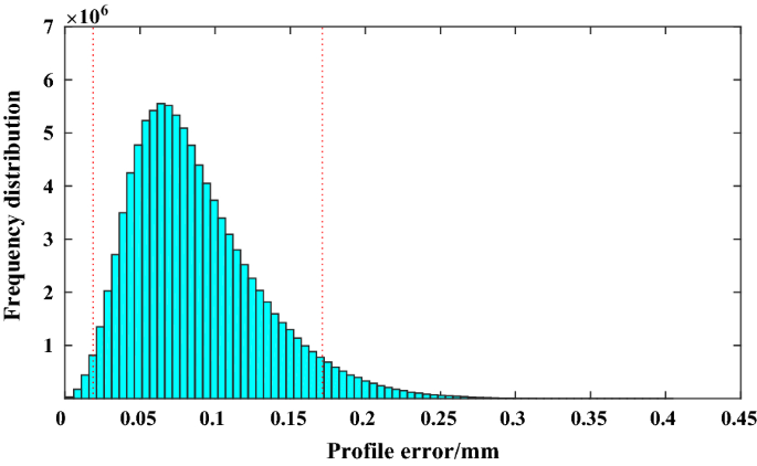
Frequency distribution of profile error in AMCM
Using AMCM, the profile error is 0.0875 mm, the uncertainty is 0.0433 mm and the confidence interval of 95% is [0.0188, 0.1714] mm.

4.2 Profile Error and Uncertainty Calculation in Experiment 2
In Unigraphics NX, adaptive placement strategy is adopted to select 50 points. It is shown in Figure 7. The CMM measures these points 100 times repeatedly.

Location of theoretical points
Using SQP, the profile error is 0.0993 mm. The best transformation matrix \(\varvec{T}(\alpha ,\beta ,\gamma ,\Delta x,\Delta y,\Delta z)\) and the nearest points \(s_{i}^{\prime } (x_{i}^{\prime } ,y_{i}^{\prime } ,z_{i}^{\prime } )\) are also obtained. The nine variables \(x_{i} ,y_{i} ,z_{i} ,\alpha ,\beta ,\gamma ,\Delta x,\Delta y,\Delta z\) have been known, the covariance and variance between the variables can also be obtained. Then GUMM and AMCM are adopted to calculate the uncertainty.
- (1)
GUMM
The uncertainties of measuring points \(ux ,\;uy ,\;uz\) are \(\overline{ux} =5.97\;\upmu {\text{m,}}\) \(\overline{uy}=0.40697\;\upmu {\text{m,}}\) \(\overline{uz}=1.3\;\upmu {\text{m}} .\) Covariance matrix of the best transformation matrix is shown in Table 5.
Table 5 Covariance matrix of \(\alpha ,\beta ,\gamma ,\Delta x,\Delta y,\Delta z\) (mm2) Based on the values, the uncertainty of the first-order GUMM is \(u1\, =\, 0.00199\;{\text{mm,}}\) the second order is \(u2 \, =\, 0.01945\;{\text{mm}} .\)
- (2)
AMCM
Refer to the principle of AMCM in experiment 1, the profile error is 0.1233 mm, the uncertainty is 0.0416 mm, the confidence interval of 95% is [0.0597, 0.2062] mm. The distribution of profile error in AMCM is shown in Figure 8.
Figure 8 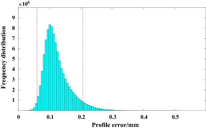
Frequency distribution of profile error in AMCM

5 Results and Discussion
-
(1)
According to experiment 1:
In GUMM, the skewness coefficient of profile error \(SK\) is 0.6287. The distribution of the profile error is asymmetrical and unknown. According to the 100 profile errors, the \(\bar{f} = 0.065574\;{\text{mm,}}\) \(Q_{0.025} = 0.05849\;{\text{mm}}\) and \(Q_{0.975} = 0.075034\;{\text{mm}}\) are obtained. According to Eqs. (15), (16), \(k_{down}\) and \(k_{up}\) are shown as follows:
$$\begin{aligned} k_{{down}} = 4 \times \frac{0.065574 - 0.05849}{0.075034 - 0.05849} \approx 1.7, \hfill \\ k_{{up}} = 4 \times \frac{0.075034 - 0.065574}{0.075034 - 0.05849} \approx 2.3. \hfill \\ \end{aligned}$$The uncertainties are calculated in the first-order and the second-order GUMM. They are written as GUMM-1 and GUMM-2 respectively in Table 6 and Table 7. The coverage probability p is 0.95. dlow and dhigh are the difference of the GUM and AMCM in 95% confidence interval. When the first-order Taylor series expansion is considered in GUMM, the values of dlow and dhigh are far larger than those in GUMM-2 (0.0419 > 0.0083 & 0.09914 > 0.0537). In a word, the second-order GUMM is more precise to calculate the uncertainty of profile error.
Table 6 Uncertainty evaluation results in experiment 1 (mm) Table 7 Uncertainty evaluation results in experiment 2 (mm) -
(2)
According to experiment 2:
In GUMM, the skewness coefficient is \(SK = - 0.4356\). The distribution of profile error is asymmetrical. Then the converge factors are shown as follows.
$$\begin{aligned} k_{{down}} = 4 \times \frac{0.099314192 - 0.089258703}{0.106076038 - 0.089258703} \approx 2.4, \hfill \\ k_{{up}} = 4 \times \frac{0.106076038 - 0.099314192}{0.106076038 - 0.089258703} \approx 1.6. \hfill \\ \end{aligned}$$In Table 7, dlow and dhigh in GUMM-2 are less than those in GUMM-1 (0.00708 < 0.0348 & 0.07578 < 0.1037). It indicates that the second-order GUMM is more precise to calculate the uncertainty of profile error.
6 Conclusions
-
(1)
When the amount of data is limited, SQP can obtain the profile error accurately and quickly. However, when the amount of data is very large, SQP is time consuming. SQP is an appropriate method according to the proper CMM data in this paper.
-
(2)
When the mathematical model of profile error is non-linear, the second-order Taylor series expansion needs to be considered. The third order or a higher-order requires the calculation and analysis of tensors, which is difficult to achieve at present. The precise prior distributions of variables in AMCM are often difficult to obtain in most cases, so the AMCM is not widely used.
-
(3)
If you want to get different confidence intervals, you need to find the corresponding endpoints of the confidence intervals. If you want to obtain the shortest 99% confidence interval, you need to sort the profile error from the smallest to the largest. Then find the location of the left endpoint n in MATLAB. Next the right endpoint f(M * 99/100 + n) is obtained, where M is the number of experiments. The 99% confidence interval in AMCM is [f(n), f(M * 99/100 + n)]. In GUMM, you need to select the corresponding converge factors (k = 3 in 99% confidence interval). The details are shown in Ref. [30].
References
Y Li, P Gu. Free-form surface inspection techniques state of the art review. Computer-Aided Design, 2004, 36(13): 1395-1417.
F Liu, G Xu, L Liang, et al. Least squares evaluations for form and profile errors of ellipse using coordinate data. Chinese Journal of Mechanical Engineering, 2016, 29(5): 1020-1028.
X Q Lei, Z B Gao, J W Cui, et al. The minimum zone evaluation for elliptical profile error based on the geometry optimal approximation algorithm. Measurement, 2015, 75: 284-288.
S Zhaoyao. Profile deviation evaluation of large gears based on NURBS surface fitting. Chinese Journal of Scientific Instrument, 2016, 37(3): 533-539.
X Yang, X L Liu, J M Liu, et al. Matching algorithm for profile error calculation of blade surface. Advanced Materials Research, 2016, 1136: 630-635.
S Xiulin, G Yang, Z Shiguang, et al. Freeform surface profile error evaluation based on gray code genetic algorithm and segmentation of spherical approximation method. Sixth International Conference on Intelligent Systems Design & Engineering Applications, Guiyang, China, 2015: 410-413.
A Lang, Z Song, G He, et al. Profile error evaluation of free-form surface using sequential quadratic programming algorithm. Precision Engineering, 2017, 47: 344-352.
Q Y Niu, Z Y Li, G H Du, et al. Geometrical product specifications (GPS): coordinate measuring machines (CMM): technique for determining the uncertainty of measurement. Measurement Techniques, 1959, 2(11): 915-919.
C X J Feng, A L Saal, J G Salsbury, et al. Design and analysis of experiments in CMM measurement uncertainty study. Precision Engineering, 2007, 31(2): 94-101.
W Kessel. Measurement uncertainty according to ISO/BIPM-GUM. Thermochimica Acta, 2002, 382(1): 1-16.
L Hui, W B Shangguan, D Yu. A unified approach for squeal instability analysis of disc brakes with two types of random-fuzzy uncertainties. Mechanical Systems & Signal Processing, 2017, 93: 281-298.
JCGM 101. Evaluation of measurement data-Supplement 1 to the “Guide to the expression of uncertainty in measurement”-Propagation of distributions using a Monte Carlo method JCGM member organizations (BIPM, IEC, IFCC, ILAC, ISO, IUPAC, IUPAP and OIML), 2008.
X L Wen, Y X Xu, H S Li, et al. Monte Carlo method for the uncertainty evaluation of spatial straightness error based on new generation geometrical product specification. Chinese Journal of Mechanical Engineering, 2012, 25(5): 875-881.
M G Cox, B R L Siebert. The use of a Monte Carlo method for evaluating uncertainty and expanded uncertainty. Metrologia, 2006, 43(4): S178.
H B Motra, J Hildebrand, F Wuttke. The Monte Carlo method for evaluating measurement uncertainty: Application for determining the properties of materials. Probabilistic Engineering Mechanics, 2016, 45: 220-228.
G Delgado. Methodology to implement adaptive Monte Carlo method in the evaluation of measurement uncertainty, using the Maple symbolic computation. Application to a simple experiment. Universitas, 2009, 3(2).
M A F Martins, R Requião, R A Kalid. Generalized expressions of second and third order for the evaluation of standard measurement uncertainty. Measurement, 2011, 44(9): 1526-1530.
X L Wen, Y B Zhao, D X Wang, et al. Adaptive Monte Carlo and GUM methods for the evaluation of measurement uncertainty of cylindricity error. Precision Engineering, 2013, 37(4): 856-864.
A Küng, F Meli, A Nicolet, et al. Application of a virtual coordinate measuring machine for measurement uncertainty estimation of aspherical lens parameters. Measurement Science & Technology, 2014, 25(9): 094011.
ISO 1101. Geometrical product specifications-geometrical tolerancing-tolerances of form, orientation, location and run-out. International Organization, 2012.
D Wang, A Song, X Wen, et al. Measurement uncertainty evaluation of conicity error inspected on CMM. Chinese Journal of Mechanical Engineering, 2016, 29(1): 212-218.
L D Oberski, A Satorra. Measurement error models with uncertainty about the error variance. Structural Equation Modeling, 2013, 20(3): 409-428.
A Chen, C Chen. Comparison of GUM and Monte Carlo methods for evaluating measurement uncertainty of perspiration measurement systems. Measurement, 2016, 87: 27-37.
M Désenfant, M Priel. Reference and additional methods for measurement uncertainty evaluation. Measurement, 2017, 95: 339-344.
R B Bendel, S S Higgins, J E T A Pyke. Comparison of skewness coefficient, coefficient of variation, and Gini coefficient as inequality measures within populations. Oecologia, 1989, 78(3): 394-400.
B R Barbero, E S Ureta. Comparative study of different digitization techniques and their accuracy. Computer-Aided Design, 2011, 43(2): 188-206.
W Wang, Z Jiang, W Tao, et al. A new test part to identify performance of five-axis machine tool—part I: geometrical and kinematic characteristics of S part. International Journal of Advanced Manufacturing Technology, 2015, 79(5-8): 729-738.
L Guan, J Mo, M Fu, et al. Theoretical error compensation when measuring an S-shaped test piece. International Journal of Advanced Manufacturing Technology, 2017, 93(6): 1-10.
A Los, J R R Mayer. Application of the adaptive Monte Carlo method in a five-axis machine tool calibration uncertainty estimation including the thermal behavior. Precision Engineering, 2018, 53: 17-25.
Y C Ni. Evaluation of practical measurement uncertainty. Beijing: China Metrology Publishing Press, 2009. (in Chinese).
Authors’ Contributions
CL wrote the initial manuscript; YS assisted with the experimental process; GH and ZS revised the manuscript. All authors read and approved the final manuscript.
Authors’ Information
Chenhui Liu, born in 1995, is currently a graduate student, majoring in probability theory and mathematical statistics at School of Mathematics, Tianjin University, China. She is now participating in projects at Key Laboratory of Mechanism Theory and Equipment Design of Ministry of Education, Tianjin University, China.
Zhanjie Song, was born in Hebei Province, China, in 1965. He received his PhD. degree from Nankai University, in 2006. He was a Postdoctoral Fellow in signal and information processing, with School of Electronic and Information Engineering, Tianjin University, China. He is currently a Professor with the School of Mathematics, a Fellow of Visual Pattern Analysis Research Lab, and a vice-director with the Institute of TV and Image Information, all in Tianjin University. His current research interests are in sampling, approximation and reconstruction of random signals and random fields.
Yicun Sang, born in 1991, is currently a PhD candidate. He is now participating in projects at Key Laboratory of Mechanism Theory and Equipment Design of Ministry of Education, Tianjin University, China.
Gaiyun He, born in 1965, is currently a professor at Tianjin University, China. She received her PhD degree from Tianjin University, China, in 2006. Her research interests include modern manufacturing quality control, evaluation methods of geometric errors and CAD/CAM/CAI integration technology.
Acknowledgements
The authors gratefully acknowledge the supports of the open fund of Tianjin Key Laboratory of Equipment Design and Manufacturing Technology (Tianjin University).
Competing Interests
The authors declare that they have no competing interests.
Funding
Supported by National Natural Science Foundation of China (Grant No. 51675378) and National Science and Technology Major Project of China (Grant No. 2014ZX04014-031).
Author information
Authors and Affiliations
Corresponding author
Rights and permissions
Open Access This article is distributed under the terms of the Creative Commons Attribution 4.0 International License (http://creativecommons.org/licenses/by/4.0/), which permits unrestricted use, distribution, and reproduction in any medium, provided you give appropriate credit to the original author(s) and the source, provide a link to the Creative Commons license, and indicate if changes were made.
About this article

Cite this article
Liu, C., Song, Z., Sang, Y. et al. An Improved Measurement Uncertainty Calculation Method of Profile Error for Sculptured Surfaces. Chin. J. Mech. Eng. 32, 90 (2019). https://doi.org/10.1186/s10033-019-0404-0
Received:
Revised:
Accepted:
Published:
DOI: https://doi.org/10.1186/s10033-019-0404-0