
Abstract
Natural source electromagnetic methods have the potential to recover rock property distributions from the surface to great depths. Unfortunately, results in complex 3D geo-electrical settings can be disappointing, especially where significant near-surface conductivity variations exist. In such settings, unconstrained inversion of magnetotelluric data is inexorably non-unique. We believe that: (1) correctly introduced information from seismic reflection can substantially improve MT inversion, (2) a cooperative inversion approach can be automated, and (3) massively parallel computing can make such a process viable. Nine inversion strategies including baseline unconstrained inversion and new automated/semiautomated cooperative inversion approaches are applied to industry-scale co-located 3D seismic and magnetotelluric data sets. These data sets were acquired in one of the Carlin gold deposit districts in north-central Nevada, USA. In our approach, seismic information feeds directly into the creation of sets of prior conductivity model and covariance coefficient distributions. We demonstrate how statistical analysis of the distribution of selected seismic attributes can be used to automatically extract subvolumes that form the framework for prior model 3D conductivity distribution. Our cooperative inversion strategies result in detailed subsurface conductivity distributions that are consistent with seismic, electrical logs and geochemical analysis of cores. Such 3D conductivity distributions would be expected to provide clues to 3D velocity structures that could feed back into full seismic inversion for an iterative practical and truly cooperative inversion process. We anticipate that, with the aid of parallel computing, cooperative inversion of seismic and magnetotelluric data can be fully automated, and we hold confidence that significant and practical advances in this direction have been accomplished.
1 Introduction and Background
Co-location of seismic and magnetotelluric surveys is becoming increasingly viable for shallow to mid-depth exploration programmes like those completed by the minerals, hydrocarbon, groundwater and hydrothermal industries. It is also increasing routinely for deeper crustal research. The challenge we identify and address is the creation and testing of practical cooperative inversion strategies intended to link information from seismic and magnetotelluric (MT) surveys to recover detailed subsurface rock property distributions.
The goal of the MT method is to recover subsurface electrical conductivity distributions from the measurement of naturally occurring electromagnetic fields. The information content residing within a co-located seismic data set should be capable of improving outcomes from magnetotelluric inversion and vice versa. To achieve mutual benefit, we should develop and if possible automate methods able to extract suitable and consequential information from the seismic data, which has a higher resolution than the MT data.
There are significant differences between the seismic reflection method and the MT method. First, high-frequency electromagnetic fields recorded by MT instruments are rapidly attenuated with depth. Consequentially, sharp geo-electrical boundaries in complex 3D settings are increasingly difficult to resolve with depth. Genuinely sharp 3D geo-electrical boundaries or high-conductivity anomalies tend to appear as highly smoothed transitional zones after conventional MT processing. Seismic reflection methods do not suffer from the same loss in resolution with depth. If used correctly, this information can potentially improve MT inversion outcomes. In an example from the Red Sea, Colombo et al. (2013) demonstrate considerable improvement of subsurface resistivity distributions after integrating seismic and MT data.
We propose several cooperative inversion strategies that have the potential to improve MT inversion results. The strategies will be tested using large co-located 3D seismic reflection and tensor MT data sets. These strategies have the potential to be automated and integrate ideas from a range of areas including: 3D MT inversion, seismic attribute analysis and geostatistics. An overview of these and other key ingredients, which may find value within cooperative or joint inversion strategies, is provided below.
1.1 An Overview of the Magnetotelluric Method
The MT method records naturally occurring electric and magnetic fields. These fields are then converted into electrical impedance and tipper values. The frequency-dependent impedance tensor Z (Simpson and Bahr 2005) expresses the ratio between electric and magnetic fields. The apparent effective resistivity, calculated from the effective invariant impedance, can then be used to visualise and validate the quality of MT data over a survey region (Berdichevsky and Dmitriev 2008). It is usually the MT-derived transverse electric (TE) and transverse magnetic (TM) apparent resistivity modes that provide a first but exceedingly basic representation of subsurface electrical conductivity distribution.
Parameters derived from the “tipper” can also be exploited in both interpretation and full 3D MT inversion. The tipper values are derived from horizontal and vertical magnetic fields (Berdichevsky and Dmitriev 2008; Vozoff 1972). An example of a parameter calculated from tipper values is the Vozoff tipper (Berdichevsky and Dmitriev 2008; Vozoff 1972). The Vozoff tipper points away from areas of higher conductivity and towards areas of lower conductivity. The tipper will be polarised linearly in 2D environments and elliptically in 3D environments. The tipper can also aid in the evaluation of complex conductivity distributions, as would be encountered across large fault systems (Berdichevsky and Dmitriev 2008). Divergence of the tipper can be explained by the Bio-Savart law (Berdichevsky and Dmitriev 2008). Both apparent resistivity and tipper value can be plotted against log frequency (z axis) or against a pseudo-depth parameter for quality control (QC) purposes to provide a preliminary impression of subsurface geo-electrical structures. Beyond the basic assessment of MT apparent resistivity and tipper values, full inversion is required.
1.2 Seismic Processing and Seismic Attributes
Once a 3D seismic survey is acquired the objective of seismic processing is usually to generate a volume of “true” relatively amplitude reflections (Yilmaz 2001a). Preservation of true relative amplitudes during processing can be challenging but is a critical element of modern seismic processing. It is needed for subsequent attempts to recover rock properties (e.g., acoustic impedance) from the seismic data (Takam Takougang et al. 2015; Virieux and Operto 2009). True relative amplitude processing is also highly desirable for the computation of seismic attributes and for optimal use of seismic information within cooperative or joint inversion strategies.
Of particular interest for our research are seismic attributes or multi-attributes that are able to identify broad subvolumes with common geological or physical characteristics that may be linked to electrical conductivity distributions. Seismic attributes can be designed to reveal or enhance structural, stratigraphic and/or reservoir characteristics that may not otherwise be apparent in the seismic reflectivity image (Onajite 2013). They can be computed from: (1) real and quadrature components of seismic data (Taner et al. 1979) and (2) the temporal or geometric relationships within seismic data (Chopra and Marfurt 2007). Attributes derived from the complex trace, such as instantaneous phase and instantaneous frequency, are routinely applied to assist seismic interpretation (Taner 2001; Taner et al. 1979).
Computation of geometric seismic attributes such as polar dip, dip angle, azimuth and curvature typically use similarity and geometric relationships between neighbouring seismic traces within a sliding window to recover estimates of the distribution of geological dip and azimuth throughout a volume (Chopra and Marfurt 2007; Tingdahl and Groot 2003). Other attributes such as semblance-based coherence and similarity may have value in detecting horizons, changes in rock properties along horizons or geological structures (Bahorich and Farmer 1995; Brouwer and Huck 2011; Chopra and Marfurt 2007; Roberts 2001; Tingdahl 2003; West et al. 2002).
The possible application of other forms of quantitative interpretation (QI) of seismic data within cooperative inversion should not be overlooked. Amplitude variations with offset (AVO), amplitude variations with azimuth (AVAz) and acoustic impedance inversion may all have beneficial roles in cooperative or joint inversion (Mahmoudian et al. 2015; Takam Takougang et al. 2015; Yilmaz 2001b).
1.3 Joint and Cooperative Inversion
Joint and/or cooperative inversion requires a petrophysical or geometric link between parameters recovered from seismic and electromagnetic methods. For joint inversion this link tends to be explicitly included in the object function to be minimised within the inversion process, as described by Haber and Oldenburg (1997). For cooperative inversion, the link tends to be implicitly included within: (1) the design of the initial or seed model, (2) the process of updating models within the inversion, or the distribution of inversion parameters (e.g., distribution of smoothness constraints). The exact mathematical mechanism used to “cross-pollinate” the inversion process with both seismic and MT information can be subservient to the underlying assumption that there is in fact physically a valid link.
Joint and cooperative inversion approaches are used to, in part, mitigate the inherent non-uniqueness of inversion (Gallardo and Meju 2004; Vozoff and Jupp 1975). We can divide joint and cooperative inversion into the broad and overlapping subcategories that dominantly rely on: (1) petrophysical relationships, (2) geometric information, (3) mutual information, (4) cross-gradient methods and (5) other methods. These are briefly described below.
1.3.1 Petrophysical Approaches
Joint and cooperative inversion of seismic and electromagnetic data may be based on a petrophysical connection between distribution of electrical and seismic rock properties. For example, formation porosity and fluid saturation can potentially be linked to conductivity in Archie’s equation (Archie 1942) and to velocity through Gassmann’s equation (Gao et al. 2012). If the porosity and/or fluid saturation are first-order drivers for the value of conductivity and velocity, then the petrophysical approach to joint inversion is reasonable. Unfortunately, formation resistivity may be strongly connected to spatial variations in the chemistry of the resident fluids. In this case the petrophysical approach would only be valid if fluid chemistry were accurately known. In porous media the degree of cementation is another parameter that can make such direct petrophysical connections problematic. A more robust approach may be to simply cross-plot velocity against conductivity from wireline logs (if available) then base the joint or cooperative inversion process on this empirically derived petrophysical relationship within suitable subdomains, as described in the work of Takam Takougang et al. (2015).
As a sidenote, the links we described between seismic and EM information required for joint or cooperative inversion should not be confused with the seismo-electromagnetic phenomena in which a tiny portion of the seismic wavefield is converted to an electromagnetic wavefield or vice versa (Dupuis et al. 2009; Garambois and Dietrich 2002).
1.3.2 Geometric Information
Geometric information can be used to guide joint or cooperative inversion (Gallardo and Meju 2004; Haber and Gazit 2013; Moorkamp et al. 2013). Geological circumstances may occur where structural links between acoustic impedance and electrical resistivity exist. For example, the vector direction of the seismic polar dip attribute extracted from a 3D seismic volume and the vector direction of maximum change in electrical conductivity (i.e. the conductivity gradient) will match for repeated conformable layering (Pethick and Harris 2014). We examine this possibility in detail later.
1.3.3 Mutual Information
Application of mutual information (MI) quantifies a distance metric between co-located images. In medical imaging, the metric can be used to align and position results from magnetic resonance imaging (MRI), computed tomography (CT) and other co-located medical data sets (Viola and Wells III 1997). Haber and Gazit (2013) applied MI inversion to two synthetic co-located data sets including direct current (DC)-derived conductivities and seismic slowness. Mandolesi and Jones (2014) applied MI to field data from the Rhenish Shield region, Central Germany. They conducted 1D MT inversion with applied MI to obtain a conductivity distribution using a reference model derived from seismic data.
1.3.4 Cross-Gradient Methods
Cross-gradient inversion attempts to minimise the difference in the vector direction of the gradients between two or more earth properties such as velocity and conductivity (Gallardo and Meju 2004). Moorkamp et al. (2013) exploited the relationship between velocity and resistivity extracted from borehole data using a cross-gradient-based joint inversion approach. Their cross-gradient based inversion imaged and characterised a salt dome.
In hydrogeophysics joint inversions of electrical resistivity and radar slowness have been applied (Doetsch et al. 2010; Linde et al. 2006). Doetsch et al. (2010) investigated the merits of structural cross-gradient methods by incorporating time-lapse cross-hole electrical resistivity tomography (ERT) data and first-arrival ground-penetrating radar (GPR) traveltimes to recover soil moisture content changes within the vadose zone.
As noted earlier, any change of pore water conductivity could prove problematic for application of strict cross-gradient methods (Linde et al. 2006). The cross-gradient approach may also prove inappropriate where clay type (e.g., high cation-exchange clays) is key driver for distribution and direction of change of electrical conductivity.
1.3.5 Other Methods
The integration of seismic boundaries can be used to build a geo-electrical framework to constrain inversion and has been applied to both passive source magnetotelluric methods (Moorkamp et al. 2007) and marine-controlled source electromagnetic methods (Harris et al. 2009). Other cooperative inversion techniques, as used by Zhou et al. (2014), apply smoothness weights at boundaries with dependence on a priori user-defined structures. That is, smaller weightings can be allocated proximal to the edge of faults or other potential geo-electrical boundaries.
In addition, deGroot‐Hedlin and Constable (1990) show that “the penalty for roughness at known boundaries may be removed in the roughening matrix”, which has the potential to permit “sharper” electrical resistivity gradients across boundaries. Conductivity models can also be engineered to support seismic inversion where a prior acoustic impedance model has aided outcomes from MT inversion (Takam Takougang et al. 2015). Here definition of prior acoustic impedance is assisted by MT inversion combined with empirical well-log relationships between electrical conductivity and acoustic impedance to image rock property distributions across a wide range of geological environments (Takam Takougang et al. 2015).
1.4 Geostatistical Methods in Cooperative Inversion
Selection and application of geostatistical methods are often of fundamental importance to cooperative inversion. Cooperative inversion generally requires the transference of information recovered from different processes such wireline logging, petrophysical measurements on core, geochemistry and outputs from inversion. These data sets will invariably have significantly different spatial resolution. The passing of information (e.g., as a constraint) derived from different methods requires some form of averaging or geostatistical grouping.
Examples of well-known geostatistical methods that may have value in cooperative inversion include basic methods such as kriging or co-kriging and clustering techniques such as k-means, Fuzzy logic, principal component analysis (PCA) and neural networking (Bedrosian et al. 2007; De Benedetto et al. 2012; Di Giuseppe et al. 2014; Dubrule 2003; Kieu and Kepic 2015; Klose 2006; Roden et al. 2015; Ward et al. 2014).
Geostatistical methods can be applied during data analysis and quality control. Basic tools of geostatistical representations at the data analysis or QC stage include histogram plots and scatter diagrams (Bourges et al. 2012; Takam Takougang et al. 2015). Variograms can be also created, and these allow the spatial distribution of parameters such as seismic amplitudes, velocity and porosity to be statistically quantified (Dubrule 2003).
Geostatistical gridding techniques such as kriging or co-kriging can also be applied to estimate values at specific locations from predicted variogram model. Bedrosian et al. (2007) use kriging to interpolate inverted MT-derived electrical resistivity values onto a finer mesh corresponding to that used for seismic velocity, to perform lithological classification. Bourges et al. (2012) demonstrate the benefits of co-kriging on the two dataset’s porosity and acoustic impedance. They found that by performing co-located co-kriging, their estimation of the key parameter, porosity, could be improved.
Clustering techniques can also play an important role in evaluating and connecting different earth parameters. k-means clustering is one such approach. k-means “minimises the sum, over all clusters, of the within-cluster sums of point-to-cluster-centroid distances” (MathWorks 2014). In an example by Di Giuseppe et al. (2014), distinct groups of resistivity and velocity are analysed by k-means for stress fault zone imaging.
Fuzzy logic is also known as a clustering approach. Fuzzy logic categorises parameter elements into several clusters, with each element assigned a membership level to each cluster (Bezdek et al. 1984; Kieu and Kepic 2015). Self-organised maps are a type of artificial neural network technique, which are able to transform multiple data sets into two-dimensional maps for identifying geology characteristics of the granitic gneisses (Klose 2006).
Many of the above geostatistical methods are broadly equivalent. In this field example, we demonstrate k-means methods.
1.5 Incorporating Seismic Information within Magnetotelluric Inversion
The failure or success of modern 3D MT inversion may be determined by the initial or seed model conductivity distribution in combination with the distribution of smoothness constraints. The prior conductivity distribution need not be complicated; however, it must create a large-scale 3D distribution of electrical conductivity, which broadly represents the true subsurface conductivity distribution.
One novel element of our research is the use of seismic attributes within automatic cooperative inversion. We will show that it is not required that the seismic attribute analysis recovers high levels of detail. Rather, we seek the geometry of subvolumes that are expected to exhibit common seismic and geo-electrical characteristics. This can be done by statistically analysing the distribution of selected seismic attributes across a large volume with the objective of capturing the geometry of a limited set of subvolumes that can later be allocated values of electrical conductivity.
Two examples highlighting the link between the characteristics that can be recovered from relative apparent reflectivity (i.e. the processed seismic volume) and the geo-electrical structure of the earth include:
-
1.
High-reflectivity boundary separating conductive cover sequences from more resistive basement: if true relative amplitude processing has been effective, then the boundary between any conductive, weakly consolidated cover and more competent, electrically resistive higher-velocity basement should be well represented. This boundary may be extracted and identified in “energy”-based seismic attributes, provided that a suitably sized sliding window is applied over the seismic volume. The energy attribute (i.e. an amplitude-based attribute) may then be used to automatically recover the geo-electrical subdivision between cover and basement.
-
2.
Repeated and continuous reflections within repeated conformable layering: such depositional environments are common in sediments. However, they also exist within certain hard-rock settings (e.g., layered intrusions, shear zones). These environments may have a common dip direction and be effectively identified by the polar dip attributes averaged over a suitably sized 3D sliding window. The polar dip seismic attribute is a geometric attribute that can be used to define large volumes with similar geological dip.
1.6 Some Guiding Principles for Cooperative Inversion
Before proceeding to describe our semiautomatic and automatic inversion strategies, we would like to summarise several caveats and considerations that may impact outcomes arising from cooperative inversion. These are listed as general principles intended to guide the development of cooperative inversion strategies and include:
-
1.
True relative amplitude processing of seismic data has been applied: for our methods we may only be seeking a limited number of geo-electrical boundaries based only on high-reflectivity boundaries such as the interface between conductive cover and crystalline basement. For example, a short window automatic gain control (AGC) should never be applied. However, in general most modern processing flows would be expected to retain the key, highest relative reflectivity interfaces.
-
2.
For the seismic volume, time to depth conversion has been completed: MT inversion operates within the depth domain. So time to depth conversion of seismic data and consequently a velocity model are required. While in many cases seismic is highly accurate, some “allowance” or “tolerance” of incorrectly located interfaces should exist in the MT inversion.
-
3.
Induced polarisation and electrical anisotropy effects may exist (Zorin et al. 2015 ) but shouldn’t unnecessarily burden the inversion: induced polarisation and electrical anisotropy in theory can certainly exist in many electrical settings. Without explicit knowledge of the existence of polarisable rocks, cooperative inversion should not be burdened with these additional degrees of freedom for full 3D inversion within a complex 3D environment. There may be value in progressively introducing these additional parameters to small subvolumes at a later stage of the inversion workflow.
-
4.
Pre-processing or parameter selection for seismic attribute analysis has been completed: our approach uses seismic attributes that are sensitive to pre-processing that will require many input parameters. These must be thoughtfully selected with the end purpose in mind.
-
5.
The size of the sliding windows selected to capture seismic information should have a scale relevant to MT methods: our approach is based on iteratively improving the prior model and updating smoothness constraints for MT inversion across key boundaries determined mostly upon seismic information. Again we should seek a limited number of well-defined subvolumes and key boundaries. We would also note that the sliding windows applied to recover or analyse seismic information can be relatively large.
-
6.
Any 3D MT prior model subvolumes should be of a geo-electrically reasonable scale with reference to depth and conductivity: the resolution of any surface-based MT method is depth dependent. There is little value to defining high levels of detail in a prior model at great depth where conductivities are not explicitly known (e.g., from wireline logging). Including geo-electrically insignificant subvolumes and/or boundaries should be avoided.
-
7.
Shallow electrical conductivities can be of the highest importance: lastly, we would like to place emphasis on the role of the shallow and often electrically heterogeneous conductivity distributions. If these shallow upper often high-conductivity subvolumes fail to be suitably included in the prior model, the inversion is doomed to failure before it starts. That is, if the shallow conductivities cannot be correctly recovered from the inversion, then artefacts are inevitable at greater depth as the inversion must somehow compensate for incorrect shallow conductivity distributions. At the other extreme, if shallow conductivity distributions are recovered in detail then the MT inversion has considerably improved prospects of recovering correctly distributed deeper conductivity distributions. We will argue that any MT inversion requiring high levels of smoothness across shallow, sharp 3D interfaces will tend to distort the representation of conductivity at depth and that cooperative inversion can help remedy this problem.
Application of our semiautomatic and automatic cooperative inversion is described next (methodology), after which a comprehensive field example, including comparison of nine inversion strategies, is provided.
2 Methodology
For this paper, our approach is to describe our cooperative inversion strategies, then apply a set of these to an industry-scale field example. The outcome will be nine 3D electrical conductive distributions stemming from the application of the nine inversion workflows. Two of these outcomes will be the results of baseline conventional unconstrained inversion and which assumes that no other information is available, and seven workflows will be cooperative inversion strategies integrating MT inversion and seismic information. Results will be presented as equivalent sets of images for comparison and analysis. The strategies are designed to span a variety of unique pathways that will enable discussion around the degree to which each strategy can be automated and/or generate a “true” representation of subsurface electrical conductivity in complex 3D geo-electrical settings containing both sharp geo-electrical boundaries and smooth transitional zones.
The estimation of electrical conductivity distribution from cooperative inversion requires the careful selection of suitable parameters through the data acquisition, pre-processing, inversion and validation stages. While success relies upon the correct selection of parameters at all stages, this research focuses on the pre-processing, inversion and data and model validation.
The MT inversion algorithm is a significant element of cooperative inversion and is the first concept we describe (Sect. 2.1). In particular, we will focus on the role of the prior model conductivity distribution and the prior smoothness constraint distribution as these are the main levers we use in our cooperative inversion. We then outline our semiautomatic (Sect. 2.2) and automatic (Sect. 2.3) cooperative inversion strategies. One premise for our research is that seismic attribute analysis can help bridge the gap between the rich information content found in seismic data and the inversion of magnetotelluric data. We outline the mechanics required to transfer seismic information to our cooperative inversion process via seismic attributes.
2.1 MT Inversion and Constraints
MT inversion attempts to recover the true subsurface conductivity distribution by minimising the residual per cent difference between the field data and simulated data. Geo-electrical model smoothness is the rate of change in conductivity between two model cells. Model smoothness plays an important role in stabilising the inversion process. deGroot‐Hedlin and Constable (1990) use the words “providing minimum possible structure” everywhere to describe the outcome of MT inversion with a single global smoothness constraint. Genuinely sharp, high-contrast geo-electrical boundaries cannot be correctly represented within such a numerical framework.
We use the ModEM code developed by Egbert and Kelbert (2012) for our experiments. Its objective function must satisfy both data misfit and smoothness requirements and is given as (Egbert and Kelbert 2012):
where m—earth conductivity model parameter, d—field data, C d —covariance of data errors, f(m)—forward modelling operator, m 0 —the initial model, \(\nu\)—Lagrange multiplier, C m —smoothing operator.
The Lagrange multiplier \(\nu\) plays a key role in balancing the misfit and smoothness requirements. C m is the model covariance or regularisation term and is also known as a smoothing operator (Siripunvaraporn and Egbert 2000). It plays a key role in dictating sharpness or smoothness between the model elements during inversion. Theoretically, each element of C m can be independently configured for all pairs of elements in m, allowing considerable fine tuning of smoothness between adjacent cells. If the elements are set to zeroes, the smoothness criteria applying to their model parameters are not included in the inversion or sharp boundary would be defined.
Figure 1 illustrates the two controls or levers that we use to drive the inversion. Seismic information can be used to assign key values for both the prior model (m 0 ) and covariance matrix (C m ). Our goals are to produce a prior conductivity model integrated with seismic structures and to populate the covariance matrix using consistent coefficients derived with the aid of seismic attributes.

Schematic illustrating the transference of seismic information to the MT inversion prior conductivity and covariance model. The correlation between a seismic, b the geo-electrical model and c the covariance model is shown. In theory, a sharp step change in resistivity can only be achieved if the component of the covariance matrix corresponding to that boundary contains a value of zero. For example, the covariance coefficient between cells B and C could be set to zero. Practically, a positive nonzero value up to around 0.25 is typically chosen. The rate of change in electrical resistivity possible between cells of the inverted resistivity model is inversely proportional to the corresponding covariance coefficient value. That is, the greater the covariance coefficient value, the smoother the boundary between cells
The prior model distribution for our cooperative inversion includes both conductivity and smoothness. The prior conductivity models may be derived from combinations of seismic information, MT unconstrained inversion and the, based on the results and drill-hole information. We will show that the prior conductivity distribution strongly influences the inversion’s outcome. Seismic boundaries can be used to create distinct subvolumes, each with uniform resistivity values, as represented by the schematics in Fig. 1. We may infer a single representative resistivity value in each subvolume by statistical analysis of the conductivities distribution recovered from unconstrained inversion within each subvolume. This approach is used to produce sharp changes in resistivity across each subvolume boundary. While this approach does not guarantee success, it is one method for automatically “loading” the prior model with reasonable conductivities within a framework recovered from seismic information.
Seismic information can also be used to assist in construction of a 3D prior distribution of smoothness constraints. That is, we assign smoothness criteria for every cell within the full model domain. The smoothness criteria can be removed or reduced at cell boundaries. Reducing the smoothness criteria at known interfaces permits the MT inversion to generate higher-conductivity gradients across subvolume boundaries.
For our example of cooperative inversion strategies, we generally select a uniform covariance coefficient within each subvolume. Covariance describes the smoothness criteria between cells, and the schematic in Fig. 1c illustrates how smoothness criteria may be assigned based on seismic information. In the schematic four cells are labelled: A, B, C and D. Cells A and B lie within region one, while cells C and D lie within region two. The assigned covariance between cells A and B (i.e. cells in the same region) should be set to high number than the covariance between B and C (i.e. cells in adjacent regions). This procedure allows MT inversion to generate a higher-resistivity gradient between B and C compared to between A and B or C and D.
For our “semiautomatic” and “automatic” strategies our approach is to initialise the covariance coefficients globally to a constant, then modify values across boundaries where the covariance is typically assigned to a smaller number (see Fig. 1). This gives the MT inversion “permission” to change more rapidly across the boundary than across cells within volumes enclosed by boundaries. We will show later that seismic attributes related to reflectivity strength along high-reflectivity boundaries can potentially be a basis for automatically defining covariance.
Seismic information, in one form or another, is used to create the framework of the prior geo-electrical model. This framework may be created in a semiautomatic way by selecting high relative reflectivity seismic horizons that are expected to be coincident with key geo-electrical boundaries (e.g., the cover to basement interface).
Alternatively, the geo-electrical framework can be built automatically with the aid of seismic attribute analysis (i.e. via statistical analysis of the distribution of seismic attributes). That is, large subvolumes exhibiting common seismic characteristics are automatically extracted from attribute images. The details of semiautomatic and automatic cooperative inversion are provided below.
2.2 Semiautomatic Cooperative Inversion
Semiautomatic cooperative inversion requires some level of interpretation. In this approach, key seismic horizons with links to geo-electrical structures must be extracted from the seismic volume. Only those horizons that are interpreted as having links to the subsurface geo-electrical features are selected. Selecting all horizons would burden the inversion process with excessive and undifferentiated information. The process is called semiautomatic because the key horizons are manually selected.
A higher level of automation may be plausible if seismic attributes can be used to auto-select relevant high-reflectivity interfaces and/or 3D auto-picking algorithms are used to recover the seismic horizons. Indeed, 3D auto-picking algorithms tend to be successful at recovering extensive high-reflectivity boundaries as is common between cover and basement within a 3D seismic volume. More specifically seismic energy, or the squared summation of seismic amplitude in a time gate, may provide a basis for classifying or “weighting” changes occurring along a boundary of high reflectivity.
Statistical characteristics, such as application of the grey-level co-occurrence matrix (Hall-Beyer 2007), may provide a volumetric tool for the classification of large volumes of earth. The energy texture attribute which is calculated from the application of the grey-level co-occurrence matrix provides a decent tool for estimating textural uniformity or defining areas of common signal character. It may also support the detection of key rock-unit boundaries or work in combination with other seismic attributes such as energy as a multi-attribute approach to volumetric classification tailored for recovering a prior model geo-electrical framework as an input to MT inversion.
Several of our example strategies will use attribute analysis to extract subvolumes with common seismic reflectivity. The next challenge is to link or assign electrical properties to these subvolumes to build the prior conductivity and/or covariance distributions necessary for MT inversion. An obvious initial approach is to search for a petrophysical relationship. Unfortunately, there is rarely sufficient data to achieve such an empirical relationship across a large variety of rock types. With respect to assigning distribution of resistivity, two important points should be considered:
-
1.
The initial or prior resistivity model serves as a guide only, intended to gently “nudge” the MT inversion in the correct direction. The inversion process itself will perform the numerical calculations to recover detailed conductivity distribution provided the starting point is reasonable.
-
2.
We never presume that any one seed model is necessarily best or correct. Equally, it would be scientifically incorrect to presume that any one final inversion outcome must be “correct” as we know there will always be equivalent models. Our approach is to create, test and compare a set of reasonable inversion strategies that may generate outcomes with equal data misfit although misfit alone may not be a good indicator of how faithfully true subsurface conductivity has been represented by the outcome of inversion.
Where there is a lack of drill-hole information, one approach that we have developed is to compute a first-pass unconstrained inversion, then based on the outcome, statistically assign a single resistivity to each subvolume within the model framework generated from seismic information. That is, the limited number of subvolumes extracted from the 3D seismic reflectivity image is allocated into a new prior model conductivity based on a statistical assessment of conductivities distribution stemming from an initial unconstrained inversion. The intent of such an approach is to provide the prior model with the general large-scale conductivity structures, beyond which the parallelised full MT inversion is called upon in the recovery of the detailed conductivity distribution.
2.3 Automatic Cooperative Inversion
For any high-quality, co-located MT and migrated seismic data sets, our “automatic cooperative inversion” presents the potential for a fully autonomous inversion process. This cooperative inversion strategy would typically involve mapping from seismic attributes to electrical conductivity.
Unconstrained MT inversion can also be used to govern a second, constrained round of MT inversion. Put simply, the large subvolumes that form a geometric framework are based on selected characteristics of seismic reflectivity as derived from attribute analysis. The electrical conductivity is then mapped into this framework, either by an inferred relationship, or with the assistance of the conductivity distribution derived from unconstrained inversion.
For the field example of automatic cooperative inversion, we will focus on possible applications for the “polar dip” seismic attribute (Brouwer and Huck 2011). This will demonstrate another of our approaches to cooperative inversion and will hopefully present readers with an approach that they may not have considered.
If averaged over a suitable window, the polar dip seismic attribute can provide a reasonable estimate of true geological dip. Depending on the seismic data quality and processing, the dip estimates tend to deteriorate at very high angles; however, subtle variations for shallow dipping rock are expected to be exceedingly well resolved. We will use the dip steering computation implemented within the OpendTect software (Apel 2001; Huck 2012) to help produce a polar dip vector seismic attribute.
The procedures for computing structural attributes are based on Fourier-Radon transformations and are fully described in Tingdahl (2003), Tingdahl and Groot (2003). The procedures require the seismic data to be initially in the time–space domain, then transferred into frequency–wave number domain and then to slowness–frequency domain. Values of slowness coordinates are linked with the maximum value by integrating over the frequency axis. Finally, polar dip is derived from the slowness coordinates corresponding to the maximum value. Other methods for computing polar dip based on complex-trace analysis are described in Chopra and Marfurt (2007). Additional detail on polar dip will be provided within Sect. 3.
There are as many potential cooperative inversion pathways as there are seismic attributes and modern parallel computing is exceedingly well suited to simultaneously testing a large numbers of inversion strategies. The set of cooperative inversions strategies we have selected aims to facilitate discussions on trade-offs between the degree to which the process can be automated, against the inversion’s ability to recover true subsurface conductive distributions, with particular emphasis on a setting with thick electrical conductivity cover sequences separated by a clear 3D cover to basement interface. These settings are increasingly important as explorers extend their search for resources to mineralised terrains that descend below deep cover (Hillis et al. 2014).
3 A Field Example
The practical value of joint or cooperative inversion strategies can only demonstrated after application to real co-located 3D seismic and MT data. We apply our semiautomatic and automatic cooperative inversion strategies to large co-located 3D seismic and magnetotelluric data sets. These data sets were acquired by Barrick Gold Corporation in one of the Carlin-style gold districts of north-central Nevada, USA. Collectively these districts represent one of the world’s premier gold-producing provinces. It is estimated that they contain approximately six million kilograms of gold, making them the second largest accumulation in the world. It accounts for 6 % of annual worldwide gold production (Muntean et al. 2011). Carlin-style gold deposits have been actively mined since 1961, although some earlier deposits were exploited at the beginning of the twentieth century (Cline et al. 2005). Palaeozoic rocks are the main host for Carlin-style gold deposits with Eocene-aged mineralisation (Cline et al. 2005; Muntean et al. 2011).
The data used for this research were collected over an area with large variations in cover thickness. Cover depths range from less than 100 m to more than 500 m, and the base of the cover sequence often has a sharp clear geo-electrical transition to more electrically resistive basement. The transition between cover and basement is an unconformity between Palaeozoic sediments that we define as “basement” and the younger “cover” sequences (Cline et al. 2005; Muntean et al. 2011, 2007; Thoreson et al. 2000).
The division between cover sequences and basement is generally well defined as a high-reflectivity interface within the seismic data (see Fig. 5e). On mass, the cover sequences tend to be more conductive than the Palaeozoic basement rocks below. The general characteristics of cover and basement sequences are:
-
1.
Drilling in the study area and the previous works (Cline et al. 2005; Muntean et al. 2011, 2007; Thoreson et al. 2000) suggest that cover rocks include unconsolidated sediments, valley-filled sediment, alluvium and interbeds of volcanics. The cover sequences are considered to be less prospective for primary gold, while basalt, mudstone, quartzite and tuff are prevalent in the Palaeozoic basement rocks. Electrical wireline logs from the study area indicate average resistivity of the order 100 Ω m for several hundred metres in basement below the Palaeozoic unconformity.
-
2.
The nature of the younger cover sequence provides a clue for the selection of seismic attribute to be used within cooperative inversion. This depositional environment is dominated by shallow dipping sequences of sand, clay, limestone and volcanics. Small changes in dip are exceedingly well defined in seismic reflectivity images and do tend to reflect significant changes in large-scale depositional environment both vertically and laterally. Further, the geometry of the cover to basement interface is clearly 3D and is also well defined in the 3D seismic image. In such depositional areas of varying dipping beds, reflection strength and polar dip can provide key constraints within a cooperative inversion workflow and we will integrate computation of these seismic attributes in several cooperative inversion strategies. Note that we do not promote that idea of a single best solution (i.e. the silver bullet) but do strongly advocate systematic analysis of outcomes from a diverse range of strategies in the context of the geological setting.
Howe et al. (2014) provide diagrams indicating the range of electrical resistivity that may be expected for the main rock types in the study area. In their research, a measured resistivity range for each major lithology group is defined. Their measurements indicate that areas with higher concentration of gold correlate with zones of higher electrical conductivity. They also provide an excellent example of MT inversion over a gold deposit.
For the MT data we completed a detailed QC process, in which every tensor MT sounding was reviewed and “cleaned”. The QC process yielded a final data set containing 213 MT stations. All inversions were completed with this same set of 213 MT records. The locations of the MT stations are shown in Fig. 2. The final data set included the impedance tensor, sampled to have 25 periods in the range of 0.0025–0.7880 s. Of the 213 MT soundings, 184 included the full tipper, sampled to have 21 periods in the range of 0.0042–0.4894 s.

a This map shows the approximate survey location as identified by the red dot. The survey was carried out in Nevada, USA. b A plan view of the 3D migrated seismic image at depth, overlaid by the location of each MT station (i.e. the blue points). The position of station 320 is highlighted by a red point, and two significant boreholes containing electrical, geochemical and geological data are identified by the yellow stars. The full processed tensor MT field record for station 320 is shown in Fig. 3
Prior to inversion it is helpful to compute the MT skin depth as a rough guide to the expected depth range of investigation. Assuming a representative resistivity in the order of 25 Ω m and MT periods in the range 0.0025–0.7880 s, the skin depth equation suggests an approximate depth range of investigation of between 150 m and 2500 m. Here we use skin depth \(\delta = 503\sqrt {\rho \cdot T}\), where \(\rho\) is electrical resistivity in Ω m and T is period in seconds. This simple skin depth analysis indicates that the inversion should not be expected to recover accurate conductivities for depths significantly less than 150 m or deeper than 2500 m.
Analysis of the tipper is helpful as it provides a coarse but important indicator of 3D geo-electrical complexity and possible large-scale zonation for later inversion (Becken and Ritter 2012; Berdichevsky and Dmitriev 2008; Tietze and Ritter 2013). Figure 3 provides an example of one full tensor record from the Nevada data set, at station identifier 320 (see Fig. 2). 3D inversion can be carried out on these data without further pre-processing. Figure 4 represents the Vozoff tippers at period 0.489 s. The Vozoff tipper vectors in Fig. 4a indicate directions of change from areas of high conductivity to areas of low conductivity. Figure 4b presents an image of the Vozoff ellipticity. The Vozoff tippers and the ellipticity are calculated from the technique described by Berdichevsky and Nguyen included within Berdichevsky and Dmitriev (2008). Zones of strong ellipticity (e.g., 0.3) are expected to occur at the boundary between two distinctly different geo-electrical settings (see dash blue line in Fig. 4b). Figure 4a, b points to a complex geo-electrical environment with large 3D changes in electrical conductivity distribution.

Processed full tensor record for station 320. The figure shows the impedance tensor, Z (a, b), the tipper mode (c) and apparent resistivity versus period curves (d, e). The components of the impedance tensor (Z) refer to the ratio between the electric and magnetic fields. The tipper mode is the ratio between horizontal and vertical magnetic fields and the apparent resistivity (Rho) and is derived from each horizontal component of tensor Z

Gridded plan views of the processed MT data at a period of T = 0.48939 s. The figure includes: a the apparent effective resistivity and Vozoff tipper induction vectors and b the ellipticity of the Vozoff tipper. A transition zone of two high and low apparent resistivity environments is highlighted by the dashed blue ellipses. The zone is also characterised by major changes in amplitude and direction of the Vozoff tippers. A zone of strong ellipticity (e.g., an approximate ellipticity ratio of 0.3) occurs within this ellipse
Above we have described the site geology, data and data quality relevant to our field example. Next we will describe the application of semiautomatic and automatic cooperative inversion strategies selected for application to the field example. The methods are selected to highlight different approaches to cooperative inversion and to facilitate comparisons between the different strategies.
3.1 Application of Semiautomatic Cooperative Inversion
Next we describe semiautomatic cooperative inversion applied to the Nevada co-located seismic and MT data. This includes description methods for building or updating both prior geo-electrical and smoothness criteria models with assistance from seismic information.
We designate strategies that require manual interpretation or inputs semiautomatic. These have limited potential for full automation. For example, where 3D seismic horizons must be manually picked the strategy is classified as semiautomatic. In the below description, we have used the OpendTect software (Apel 2001; Huck 2012) for picking horizons from the Nevada seismic volume.
3.1.1 Selection and Application of Seismic Attributes for Cooperative Inversion
As noted in Sect. 2.2 seismic attributes such as seismic amplitude, energy and energy texture can aid selection and classification of key seismic boundaries or subvolumes with common seismic and possibly geo-electrical character. Figure 5 presents images of several seismic attributes along and key horizons picked from the seismic volume (i.e. Fig. 5e). Figure 5b–d represents the large-scale distribution of the seismic attributes calculated from seismic data (Fig. 5a) as energy, energy texture and dip angle, respectively. Each attribute provides the opportunity to subdivide the full seismic volume into a set of subvolumes.

Seismic inline and cross-line slices extracted from the 3D seismic volume showing various seismic attributes within the Nevada survey area. These seismic attributes were selected to highlight various structural features. The figure includes a migrated seismic lines, b seismic energy attribute for highlighting strong reflectors, c energy texture for defining subvolumes with common seismic texture and d dip angle extracted from polar dip for identifying subvolumes based on structure. e Identifies major structural features coherent across each of the seismic attributes. The white line demarcates the basement and upper sediments
A notable horizon is highlighted by the white line in Fig. 5e. It likely represents a key geological unconformity with strong acoustic impedance and geo-electrical contrast. The yellow and blue lines represent key, high-reflectivity horizons within cover sequences. These sequences are later shown to enclose higher-conductivity rock types. The rock types vary rapidly in both vertical and horizontal directions.
3.1.2 Creation and Update of the Prior Conductivity Model
Creation and update of the prior conductivity distribution is a practical and consequential part of full inversion and analysis of MT data. The set of images in Fig. 6 show the steps used to create prior conductivity distributions for our semiautomatic cooperative inversion strategies. For the field example only the highest reflectivity boundaries are extracted from seismic attribute volumes (e.g., based on amplitude and reflective energy) to build a prior conductivity model for MT inversion. These horizons are likely to represent key geo-electrical boundaries (Fig. 6a).

Workflow for the semiautomatic inversion strategy. The workflow consists of three steps: (1) interpolate horizons from initial picked points (a), (2) select the representative conductivity in the regions defined between the interpolated horizons (b) and (3) assign this conductivity to each subvolume to generate an sharp prior model (c). The conductivity model, b, is generated from an unconstrained MT inversion starting from a 40-Ω m half-space prior model. A smooth boundary prior model (see d) is generated by smoothing the sharp model (c) with an averaging 3D box filter, 3-by-3-by-3 in size
For the Nevada example, we have reduced the full conductivity distribution derived from unconstrained MT inversion to just five conductivities (i.e. 40, 30, 20, 35, 100 Ω m). These five values are then mapped to the appropriate subvolumes, as shown in Fig. 6c. Note that unconstrained inversion, initialised with a 40-Ω m half-space prior model, provides a basis for assigning conductivity within each of these five large seismically derived subvolumes. As is commonly the case, there is insufficient wireline log data to build a petrophysically based prior conductivity model.
The lower half-space subvolume is considered as a special case when assigning a value for the conductivity prior model. Neither seismic nor MT can provide a reasonable estimate over the full lower subvolume, which has no lower boundary. We use a value of 100 Ω m in the “basement” rock as it is consistent with the average resistivity from wireline logs immediately below (i.e. within 200 m) the cover to basement interface.
By explicitly limiting the prior model to five conductivity values we have created a starting model for inversion with sharp well-defined transitions between each seismically defined subvolume (Fig. 6c). There will always be a degree of uncertainty as to the exact boundary placements. Therefore, a 3D smoothing filter is applied to “soften” each boundary, generating a second smoothed conductivity prior model (see Fig. 6d). The filter is a 3-by-3-by-3 box filter with usage defined by the MATLAB (version R2014b) built-in code, smooth3.m.
3.1.3 Creation and Update of the Prior Covariance Model
The prior covariance coefficients must be assigned across all cells (see Eq. 1). Kiyan et al. (2014) illustrate inversion with different covariances in synthetic data to evaluate the extent and conductivity of a 2D conductor. They found that the default covariance model with 0.3 gave an acceptable result. Similarly, we find that a covariance coefficient of 0.3 in all directions is generally suitable for unconstrained inversion strategies.
For semiautomatic cooperative inversion, the distribution of the covariance coefficients is uniform (i.e. 0.3) within subvolumes and reduced across subvolume boundaries. The obvious question is what value of covariance coefficient should be set across subvolume boundaries. To answer this question, we complete a small semiempirical study where we run 3D MT inversion with different covariance coefficients set across the key geo-electrical interfaces. We then assess how representative the resultant conductivity changes across the interface in the vicinity of a deep drill hole. The test is completed with the resistivity prior model shown in Fig. 6c which includes clearly defined horizons. MT inversion is completed with covariance coefficients set across the key boundaries at 0.00, 0.10, 0.20, 0.25, 0.27 and 0.30.
The results of these covariance coefficient tests are captured in Fig. 7. A coefficient of value 0.3 at boundaries means that no seismic horizon is recognised in the covariance model (i.e. 0.3 everywhere). Figure 7 includes a seismic reflectivity image showing three key horizons in the cover (i.e. marked in cyan) and the main horizon representing the cover to basement interface. The panel to the right of the seismic image shows the six different inverted conductivity curves and a wireline conductivity log at the position of well 1.

Image illustrating the consequence of using six different covariance coefficient values across four selected seismic horizons within 3D MT inversions of the Nevada MT data. The left panel provides a greyscale seismic reflectivity image (i.e. section view) along with the four picked seismic horizons and the well location. The strong lower horizon marked in magenta is the interface between cover and basement. The right panel provides a comparison of conductivity distribution at the well location after inversions with covariance coefficients set to 0, 0.1, 0.2, 0.25, 0.27, and 0.3. Setting the covariance coefficient to 0 across the boundaries of the high conductivity central layer tends to result in “overshoot”. In contrast we suspect that leaving the covariance at 0.3 everywhere may “over-smooth” what are likely to be sharp high geo-electrical contrast boundaries. After analysis of the results we have taken a value for the covariance coefficient of 0.25 across the key seismic horizons to be a reasonable compromise
We observe that the inversion results where covariance coefficients across boundaries are set at 0.2 or less tend to overshoot at the interfaces of the high-conductivity layer. Results where values were set at 0.27 and 0.3 could be considered over smoothed as boundaries are expected to be sharp. The curve with a covariance of 0.25 (red) was selected as providing the optimal smoothness across geo-electrical boundaries. It provided the best match to the picked horizons while also maintaining the high conductivity value within most conductive layer. After considerable trial and error, we concluded that covariance coefficients between 0.25 and 0.30 tended to generate stable results. Later we will consider semiautomatic strategies with:
-
1.
Uniform covariance values throughout the full model domain (e.g., a global constant covariance coefficient of 0.3).
-
2.
A reduced covariance value across all subvolume boundaries (e.g., a global constant covariance coefficient of 0.3 is set everywhere except at subvolume boundaries where a value of 0.25 is used).
3.2 Application of Automatic Cooperative Inversion Strategies
Given a valid seismic reflectivity volume and co-located MT data after QC, those strategies with potential to be fully automated are classified as “automatic cooperative inversion”. For example, structural or amplitude-based attributes may be selected to automatically partition the full model domain into subvolumes. These partitions may then be automatically allocated resistivities according to a pre-defined set of rules. We will also show that considerable success can be achieved by allocating a limited number of plausible electrical resistivities based on a statistical analysis of first-pass unconstrained MT inversion (another process with potential to be fully automated).
3.2.1 Application of the Seismic Polar Dip Attribute in Cooperative Inversion
Geological dip is a fundamental characteristic of any geological setting. Under certain circumstances, the dip of formations, layering, bedding, faults or shears, can be extracted from seismic data via the “polar dip” seismic attribute. If used with care, the polar dip attribute can play a central role in building prior models for cooperative inversion.
Figure 8 provides a schematic representation for true polar dip. Polar dip can be particularly useful in differentiating extensive shallow dipping subvolumes. At the other extreme the polar dip attribute can be either inaccurate or provide little to no value in differentiating volumes of massive crystalline rock and/or steep-dipping intrusive bodies.

Illustration of the seismic polar dip vector modified from Nelson (2009). The vector direction of polar dip attribute is the vector \(\overrightarrow {(n}\)) oriented normal to the seismic structure (i.e. bedding) (Pethick and Harris 2014). The dip angle, Ө, is the inverse tangent function of the polar dip attribute
For our research, we always apply dip steering with the fast Fourier transform algorithm available within the OpendTect software for recovery of structural attributes like polar dip. Methods for recovering structural attributes are also described in Tingdahl (2003), Tingdahl and Groot (2003) and Chopra and Marfurt (2007).
Typically, the polar dip attribute is given in units of milliseconds/metres if derived from seismic images in time or metres/metres for depth-converted seismic images. Put simply these structural seismic attributes are based on a ratio between a vertical and horizontal distance for sufficiently similar seismic events (dGB Earth Sciences 2015). For our research, we converted the seismic polar dip attribute in metre/metre to a dip angle attribute in degrees.
We will provide several examples of automatic cooperative inversion that uses the polar dip seismic attribute to assist populating prior model subvolumes with electrical conductivity. For our Nevada example, the dip angle attribute is used to group large volumes within the cover sequences. Here we expect large packages of rock with common depositional and structural history to have common geo-electrical properties.
3.2.2 Application of Automatic Strategies for Mapping Seismic Attributes to Conductivity
Processes that can be automated present a possible efficiency dividend. We explore methods for automatic mapping of geo-electrical properties into large subvolumes with common seismic character. We will demonstrate two possible directions for automatic cooperative inversion. The first method is a direct mapping from a seismic attribute value to a limited number of electrical conductivities. The second method uses statistical analysis of the spatial distribution of both seismic attribute values and electrical conductivity-derived unconstrained MT inversion.
3.2.2.1 Direct Mapping
For our Nevada field example, we use a fast, gross automatic direct mapping of the seismic dip angle attribute to a limited number of electrical conductivities within the cover sequences. The logic followed here is that extensive subvolumes containing common dip angle are likely to have common depositional and structural histories, which is a simple reasonable criterion for large-scale geo-electrical grouping within the cover sequences. No attempt is made to extend this direct mapping to the much older basement subvolume (i.e. the lower half-space) where dip angle based on seismic is poorly resolved.
A schematic illustrating direct mapping of dip angle to resistivity is shown in Fig. 9. When viewed at a large scale, a relationship between dip angle and electrical resistivity distribution derived from unconstrained inversion in the cover certainly seems to exist (Pethick and Harris 2014). The direct mapping relies on grouping of dip angle into a limited number of clusters then mapping resistivity into these subvolumes based on a simple rule. For example, within cover thick layers with uniform shallow dip tend to be more conductive than areas with higher dip angle.

Schematic illustrating model generation during automatic cooperative inversion. This is based on directly mapping conductivities into a geometric framework as defined by common seismic attribute analysis. For the Nevada example, the dip angle attribute was chosen. This process relies on a broad link between the seismic attribute and the large-scale geo-electrical structure of the earth
A strategy that directly maps conductivities based on dip angle is not going to be universally applicable. However, under suitable conditions (e.g., within conductive cover), it can be a component of an effective and fully automatic strategy for setting up a prior conductivity distribution for MT inversion, especially where no other constraints are available. We reiterate that for our Nevada example an objective is to create a set of reasonable prior model conductivity distributions where little or no information other than the seismic and MT is available.
While we observe these large-scale relationships between areas of common dip angle in cover and electrical conductivity for the Nevada example, such relationships are by no means universal and should be assessed on a case by case basis. One clear advantage of this method is its simplicity. Once the broad geo-electrical structure is set it is the inversion (run on a supercomputer) that will hopefully arrange conductivities in detail via minimisation of misfit between field data and model data (see Eq. 1, Sect. 2.1). Posterior analysis of inversion statistics and more directly conductivity distribution should be compared for the full set unconstrained and cooperative inversion strategies completed.
3.2.2.2 Statistical Mapping-Based Seismic Attribute Subvolumes and Unconstrained MT Inversion Conductivity Distribution
For the second and perhaps more universal automatic cooperative inversion technique, we use k-means clustering of the average dip angle seismic attribute to form a small number of subvolumes based on dip angle “groups”. These large subvolumes form an initial “empty” framework.
Each subvolume needs to be filled with a sensible discrete electrical conductivity. The discrete conductivity can be extracted via analysis of the conductivity distribution recovered from unconstrained MT inversion. The intended outcome is a prior conductivity model that has both seismic and MT characteristics. This prior model is then passed to a new round of MT inversion, which we run on a Cray Cascade system at the Pawsey Supercomputing system in Perth Western Australia.
We have produced a schematic as Fig. 10 to explain how conductivity from unconstrained inversion can be mapped into seismic attribute subvolumes. The methods indicated in Fig. 10 can be compared with that for direct mapping in Fig. 9.

Schematic illustrating automatic cooperative inversion based on mapping conductivity from unconstrained inversion into geometric framework defined by statistical analysis of the distribution of seismic attributes or multi-attributes. In short the prior model framework is derived from seismic information and the discrete conductivity value for each subvolume through unconstrained inversion. In principle, any attribute or combinations of attributes can be used. However, for the Nevada example the subvolumes framework is recovered from statistical analysis of the distribution of the seismic dip attribute in the cover. From the schematic it is clear that a group with a common seismic characteristic (i.e. group 1) can be populated with completely different electrical conductivities. This is a highly significant difference with the automatic cooperative inversion based on a direct mapping illustrated in Fig. 9. We should reiterate that only large subvolumes are used to create the prior conductivity model after which full 3D MT inversion is applied to recover detailed conductivity distribution and associated fitting error statistics for comparison with other strategies
Below we will systematically work through the main steps as illustrated in the schematic in Fig. 10 as applied to the Nevada field example.
- Step 1:
-
Establish a subvolume framework based on analysis of the seismic dip angle attributes (see Fig. 10a):
First, the seismic dip angle attribute is computed. Its three-dimensional distribution is then statistically simplified into a finite number of spatial groupings. Here the number of dip angle groups is decided by analysing a histogram of dip angles extracted from the seismic attribute volume. The histogram for the Nevada seismic volume is provided as Fig. 11a. Spatial sampling within the seismic volume is orders of magnitude greater than that required for the MT finite element mesh, so resampling onto nodes of the MT conductivity model finite difference mesh is required, as shown in Fig. 11b. For the Nevada data set, four distinct average dip angle groups can be recovered from the observed dip angle histogram resampled into the MT model domain. These include the dip angle in the ranges: (1) 0°–12°, (2) from 12° to 25°, (3) from 25° to 40° and (4) from 40° to 80°. A k-means clustering algorithm (i.e. MATLAB built-in code, kmeans.m) is then applied to categorise all observations of dip angle into the five predetermined clusters in which each observation belongs to the cluster with the nearest mean. This nearest mean represents the characteristic value of the cluster or group. The five average values within each group were found to be 10, 20, 27, 58 as shown in Fig. 11c, and value representing maximum dip angles is located at 83°. These group means correspond to the index numbers 1, 2, 3, 4 and 5. In summary, this first step takes a complex distribution of seismic dip angle attribute values and simplifies this into five classes, each with its index number. Note that for this strategy it is possible to have many separated 3D zones having the same index category.
Fig. 11 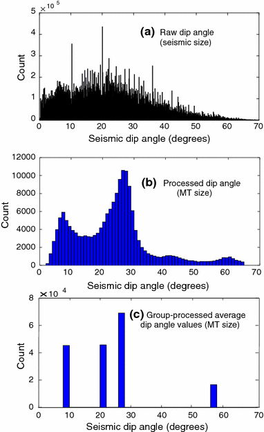
Histograms of the seismic dip angle a at the seismic scale and b in MT model domain and c dip angle derived from k-means grouping. a Histogram expressing distribution of the seismic dip angle attribute from the full seismic volume (total number of samples in the seismic volume = 4.5343E + 09). It should be noted that the histogram is computed at a finer resolution than that of the MT. b The histogram after processing the seismic dip angle volume at MT model resolution. This is performed by averaging the values in each MT subvolume (total number of cells = 173,387). The depth size of each 3D subvolume increases according to depth. This explains why the shape of MT-sized distribution of dip angle is grossly similar to the seismic-sized distribution of dip angle. c The resulting histogram after applying a k-means clustering method. Five groups are generated after it is applied to the dip angles seen in b. The seismic area is smaller in extent than the MT volume and must be padded by any specific number (i.e. the maximum dip angle value). In this case, the four groups with blue bars extracted from seismic dip angle information (b) and one red-bar group is set by the manually padded group (total number of cells = 223,776)
- Step 2:
-
The last step is to assign conductivity distributions into closed subvolumes defined by analysis of seismic attribute distributions (see Fig. 10c)
The second step is to compute unconstrained MT inversions to establish a first-pass background electrical conductivity distribution. This first-pass conductivity distribution is necessary to assist in the mapping of discrete conductivity values into the subvolumes recovered from seismic information. It may be necessary to commence unconstrained inversion with several different half-space resistivities.
- Step 3:
-
In this step each subvolume, with characteristic dip angle attributes, is allocated with a value of conductivity. The method we use is to average all values of electrical conductivity resulting from unconstrained inversion in each subvolume. This average value in each subvolume becomes the single conductivity for that subvolume within the prior model. Finally, a smoothing convolution filter (i.e. a box filter) is applied to the resulting 3D conductivity distribution. This approach accommodates subvolume boundary locations that may be approximate. It is the position of each mean dip angle subvolume that helps to form the model skeleton in which one average conductivity value represents one 3D separate closed zone. Histograms of conductivity distribution are shown in Fig. 12 for unconstrained inversion (Fig. 12a), sharp automatic (Fig. 12b) and smooth automatic (Fig. 12c)
Fig. 12 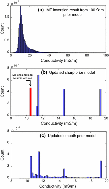
Histograms of conductivity derived from unconstrained inversion and seismic dip angle information. a The histogram showing the distribution of conductivities computed by an MT unconstrained inversion from 100-Ω m homogenous half-space prior model (total number of cells = 223,766). b The updated sharp prior conductivity model histogram after grouping the conductivities by those established through the k-means clustering of dip angle shown in Fig. 11c (total number of cells = 223,766). The blue bars show conductivity extracted from seismic dip angle and unconstrained inversion conductivity. Again, the red bar shows conductivity locating outside seismic area in which dip angle could not be computed. c The updated smooth prior model histogram of conductivity (total number of cells = 223,766). It is created by smoothing the sharp conductivity model (e) with an averaging 3D box filter, 3-by-3-by-3 in size


For the Nevada field example, the prior conductivity distribution is shown in Fig. 13 and the steps taken to build the prior conductivity distribution for this second automatic cooperative inversion option are summarised. It should be noted that the resulting prior conductivity models (i.e. see Fig. 13e) after grouping share the similar structure seen in the dip angle attribute volume (i.e. see Fig. 13c).

Images representing the steps taken to create the conductivity prior model for an automatic cooperative inversion strategy. The figure shows a a migrated seismic image, b a raw dip angle seismic attribute image, c the dip angle volume after rescaling to MT resolution and application of k-means clustering, d the conductivity distribution resulting from unconstrained MT inversion based on a 100-Ω m half-space and e the resulting prior model conductivity distribution ready final MT inversion. The resulting conductivity volume should reflect the structures found in the seismic while maintaining a reasonable conductivity distribution. Our geometric mapping method has one significant advantage. That is, subvolumes with similar seismic character can be used to automatically allocate separate individual regions of conductivity in the prior model as would occur if the same formation was physically separated (e.g., by faulting) or had regions of different solute concentrations
3.3 Preparation and Analysis of Nevada Drill-Hole Logs and Geochemical Data
Drill-hole data are precious. It presents one fundamental method for assessing the outcome of inversion. Comparison of inversion outcomes along drill holes can be based on geological logging, wireline logs and/or geochemical analysis. For the two reference drill holes located at the Nevada site, we have used geostatistical methods to divide the rock into classes based on a suite of geochemistry elements. For the geochemical data, PCA and k-means clustering techniques have been used to reduce the data dimension to highlight a limited number of geochemically similar rock types (Alférez et al. 2015; Grunsky and Smee 2003; Jolliffe 2002; Nanni et al. 2008; Roden et al. 2015). The purpose of the analysis was to check the consistency of geochemical groupings with seismic boundaries, prior model conductivity distributions and the final conductivity distribution from semiautomatic and automatic cooperative inversion strategies.
First, we removed high noise data (e.g., elemental concentration that are negligible) and then used simple range scaling from 0 to 1, as suggested by Samarasinghe (2006). We then applied principal component analysis based on 15 elements to extract nine components after which the k-means algorithm was applied to group these new components.
Note that we broadly follow the methodologies expressed in Roden et al. (2015), with the main difference being that Roden et al. (2015) used self-organising maps (SOM) for clustering, while we use the k-means method (Alférez et al. 2015; Nanni et al. 2008). The end result of the analysis of bore hole geochemical analysis is a limited number of geochemical classes.
In the “Results” section below we will compare lithology, well-log data and geochemical clusters to seismic boundaries, and conductivity distribution obtained from cooperative inversion strategies at the two reference drill-hole locations.
4 Results
In Sect. 2, automatic and semiautomatic cooperative inversion strategies were described. This was followed by description of the application of semiautomatic/automatic cooperative inversion with the aid of a field example from Nevada, USA. In Sect. 4, we will describe, analyse and compare the outcomes from application of nine MT inversion strategies.
Note that multiple strategies were run simultaneously on the Magnus supercomputer located at the Pawsey Supercomputing Centre in Perth, Western Australia. Run times for each strategy were of the order 24 h on the Cray Cascade system. Pethick and Harris (2016) provide a detailed account of applied parallel computing for EM methods. They include analysis of speed up and wall time for standard Intel processors versus the optimised Cray Cascade system that was also used for the current research.
There are limitless combinations of seismic attributes and MT inversion methods that could be attempted. We elected to systematically work through nine strategies we label S1–S9. These strategies were selected to facilitate comparison of misfit and final inverted conductivity distribution for: conventional unconstrained inversion (S1–S2), automatic cooperative inversion (S4–S6) and semiautomatic cooperative inversion (S3, S7–S9).
The “base case” unconstrained inversions are named S1 and S2. The seven cooperative inversion strategies, S3–S9, use seismic information to aid development of the prior model conductivity distribution, (m 0 ) and/or covariance matrix values, (C m ) needed for input to subsequent rounds of 3D MT inversion (see Eq. 1). We have organised the main points that differentiate these nine inversion strategies into summary in Table 1 and provide more complete descriptions below.
4.1 Unconstrained Inversion (S1–S2)
For the first two strategies, S1 and S2, the half-space prior model resistivity is set to 100 and 40 Ω m, respectively (see Table 1). The value 100 Ω m (S1) is selected to be consistent with the average wireline log resistivity measurements immediately below cover (i.e. in basement). The value 40 Ω m (S2) is selected to be consistent with the gross resistivity of the younger cover rocks above basement. Strategies S1 and S2 use a uniform covariance coefficient of 0.3.
4.2 Semiautomatic Inversion (S3)
Strategy S3 is identical to the unconstrained inversion strategy S2, except that for strategy S3 the covariance coefficient is reduced from 0.3 to 0.25 for cells that cross key high-impedance contrast interfaces picked from the seismic volume. An example of a high acoustic impedance interface is the boundary between cover and basement.
4.3 Automatic Cooperative Inversion (S4–S6)
Automatic cooperative inversion strategies can, in principle, be automated. For the Nevada field example, the structural seismic attribute, dip angle, is used to create the geometric framework (see Sect. 3.2). However, the ideas presented can certainly be adapted to take advantage of other seismic attributes or combinations of attributes.
Strategy S4 uses “direct mapping” of the seismic dip angle attribute to electrical conductivity distribution for the prior model (see schematic in Fig. 9). Direct mapping is in essence a mapping of some characteristic extracted from the seismic data to an electrical conductivity. This mapping is usually based either on a presumed or empirically determined petrophysical relationship possibly established by cross-plot of velocity and conductivity from wireline logs.
Given enough wells and good quality wireline log data a neural network approach could, in principle, be adopted to build nomogram connecting parameters derived from seismic and electromagnetic data (Bauer et al. 2012). However, as with the Nevada example, there is rarely sufficient log data to build the relationships.
Strategies S5 and S6 use the distribution of dip angle to divide the complete seismic volume into smaller subvolumes with a common seismic character. Each subvolume is subsequently assigned an electrical resistivity based on analysis of the distribution of conductivity derived from unconstrained inversions S1 and S2, respectively (see Fig. 14). We call this type of mapping from unconstrained inversion into a framework defined by seismic information “geometric mapping”.

Image representations of the prior model conductivity distributions for cooperative inversions applied for the Nevada field example. Each image includes an elevation slice at 610 m below average ground level for the study area. These prior model conductivity distributions are created according to the methods outlined in Table 1, where inversion strategies S1–S9 are outlined. a and b are included as reference images of seismic amplitude the polar dip attribute, respectively. c Prior conductivity model for strategy S4 (i.e. direct mapping), d, e prior conductivity distributions for automatic cooperative inversion strategies S5 and S6, respectively (i.e. geometric mapping). g, f Prior model conductivity distribution for semiautomatic cooperative inversion strategies S7 and S8, respectively. The prior models for strategies S8 and S9 are identical; however, for strategy S9 the covariance coefficients are reduced for cells that cross geo-electrical boundaries. The key point from this figure is that there are many valid pathways for creating the prior model conductivity and covariance coefficient distribution. While all models do have a common gross distribution, details clearly vary from model to model. Figure 15 shows how these differences impact on the final conductivity distribution for each cooperative inversion strategy
For the Nevada example, five classes of subvolumes are created based on k-means cluster analysis of the distribution of the dip angle seismic attribute (see Fig. 11c). A resistivity value is then assigned to each subvolume by statistical analysis of the conductivity distribution derived from unconstrained inversion using half-space models of 100 Ω m (S1) and 40 Ω m (S2). In this way the seismic information provides a geo-electrical framework and the unconstrained inversion is used to generate a discrete conductivity that is assigned to each subvolume. It should be remembered that the prior model needs only to have a simple relatively gross and broadly correct 3D conductivity distribution for the subsequent rounds of inversion to yield a vastly improved final outcome.
4.4 Semiautomatic Inversion (S7–S9)
Cooperative inversion strategies S7–S9 are designated semiautomatic because the key seismic boundaries that form the geo-electrical framework were picked by a partly manual and subjective process. For these strategies seismic attributes like amplitude, energy and energy texture were highly useful in identifying key horizons. After identifying key horizons, an auto-picking algorithm (Huck 2012) was used to recover them through the seismic volume. The auto-picking tended to be successful for recovery of the main high acoustic impedance contrast horizons. The result is that the seismic volume was readily partitioned into large subvolumes that ultimately formed a prior geo-electrical model framework for S7, S8 and S9.
The prior model framework for semiautomatic cooperative inversion strategies S7, S8 and S9 included just four interpreted horizons (see Fig. 6a, b) and five large subvolumes. The largest subvolume was the lower basement half-space. A resistivity was assigned to each of the other subvolumes by “geometric mapping” (see Fig. 9) based on statistical analysis of resistivity distribution derived from unconstrained inversion using a 40-Ω m half-space model (see strategy S2). The four subvolume resistivity values assigned to the cover rocks were 40, 30, 20 and 35 Ω m. A resistivity of 100 Ω m was mapped into the full basement subvolume because it is broadly consistent with outcome from unconstrained inversion (S1) and wireline log resistivity (see Sect. 3.1.2) immediately below cover.
Figure 14 provides an image representation of the original seismic reflectivity, the dip angle seismic attribute distribution and prior models conductivity distributions for cooperative inversion strategies S4–S9. The nine strategies are included to compare advantages and disadvantages of inversion strategies.
We immediately see that automatic cooperative inversion strategies S4–S6 permit prior model conductivity detail within basement that is not permitted for semiautomatic strategies S7–S9. For strategies S4–S6, the geo-electrical framework comes directly from the volumetric distribution of a seismic attribute whereas for S7–S9 the framework is based explicitly on selected seismic horizons. One approach is likely to provide accurate 3D geo-electrical boundaries, while the other provides an objective, mapping conductivities onto subvolumes with common seismic character.
4.5 The Final Conductivity Distribution for Inversion Strategies S1–S9
Next we provide final conductivity distributions for inversion strategies S1–S9 and analyse these outcomes with respect to fitting errors, the original seismic reflectivity and drill-hole data. A representation of final conductivity distributions from inversion strategies S1–S9 are provided in Fig. 15. All nine final inverted conductivity models broadly represent the geometry of the more conductive cover. However, as anticipated there are considerable differences in the distribution of conductivity in cover and below cover between the nine different strategies.

Image representations of the final 3D electrical conductivity distributions after application of MT inversion strategies S1–S9 (see Table 1). Each image shows an elevation slice at 610 m below average ground level for the study area. The white lines represent the key boundary between basement and covers rocks. Note that inversion strategies S1–S3 all fail to recover a higher-resistivity basement ridge protruding into cover on the right of these images. This ridge is clearly mapped within the seismic reflectivity volume. This ridge is clearly resolved in strategies S7–S9. While strategies S7–S9 have exceptional resolution in cover, strategy S4 appears to resolve linear features in basement on the left-hand side of the images. Our example is intended to highlight the possibly uncomfortable reality that no single strategy will adequately recover conductivity distribution across a large volume containing diverse geo-electrical settings
We will return to the analysis and comparison of these conductivity distributions after considering model convergence and data misfit for the nine inversion strategies.
4.6 Assessing Inversion Strategies S1–S9: Convergence And Misfit
For each 3D MT inversion strategy, a suitable error floor needs to be specified. The error floors for off-diagonal elements (Zxy and Zyx) are set to 5 % of the root mean square (RMS) absolute of their complex multiplication. Diagonal elements (Zxx and Zyy) share the same error floor with the off-diagonal elements because both are small and tend to be noisy. The error floor of tipper values is set to 0.02.
Assessing the fit between field and synthetic data is not straightforward. The rate of convergence for inversion strategies S1–S9 is shown in Fig. 16, and details are included in Table 2. At a basic level we could consider rate of convergence and global RMS error as indicators of the relative success for each inversion. However, this would be misleading and further analysis is required.

Total root mean square misfit error at each inversion iteration step for each of the nine inversion strategies (S1–S9). The fastest rate of convergence and lowest global RMS misfit is achieved with automatic inversion strategy S6. However, all RMS misfits are between 1.65 and 1.33, which is exceedingly low. A closer investigation of misfit is required
The global RMS error (Table 2) alone is a blunt instrument for analysing fit, which can be assessed for each sounding. Figure 17 shows a complete representation of field data and final inversion outcomes from all strategies for tensor MT station 320. The location of station 320 is provided in Fig. 2. The inversion strategies S1, S2 and S3 using half-space prior models generally do not achieve the rate of change observed in the field MT apparent resistivity curves. This is likely because unconstrained inversion strategies S1 and S2 do not contain the information necessary to accommodate high geo-electrical contrasts in their prior models. These high geo-electrical contrast interfaces are accurately located in the seismic volume, and this information is transferred to the MT inversion by different methods in strategies S4–S9.

Comparison of field MT data and final computed model MT data resulting from nine inversion strategies for MT station 320 (see Fig. 2). The apparent resistivity and phase for Zxy and Zyx fit exceedingly well to the MT data generated at the end of most inversion strategies (see fit for strategy S9). As expected the signal to noise levels in the Zxx and Zyy component data are exceedingly low and as such a close fit is not anticipated (i.e. some elements of the data are not reliable)
A different way to assess the nine inversion strategies is to compare apparent resistivity and tipper values of the real field and synthetic data at each period for all MT stations that were included in inversion strategies S1–S9. In Fig. 18 we show a map of apparent resistivity and tipper at period of 0.092367 s for the nine inversion strategies. Figure 18 shows that the model apparent effective resistivity for all strategies is similar to the field values. However, Vozoff tipper directions at the measurement area edge tend to diverge from the tipper derived from the field data.

Ten plan view slices of MT apparent effective resistivity and Vozoff tipper vector at a constant period (0.092367 s), providing a direct comparison of the real field data and synthetic MT data after application of inversion strategies S1–S9. The difference between field and model derived tipper vectors tends to increase towards the model boundaries where both seismic and MT coverage ends
Figure 19 shows residuals between synthetic and field data at the same period for the nine cooperative inversion strategies. This provides a better diagnostic of the quality of the fit between modelled and real data than the global RMS value. Localised, high misfit areas can be readily identified.

Plan view slices of percentage residuals (i.e. synthetic data subtracted by the field data as a percentage normalised by the field data) of the abs(Zyx) at a constant period (0.092367 s) for all inversion strategies. Per cent residuals from the automatic and semiautomatic cooperative inversion strategies demonstrate a reduction in zones of high local misfit that is apparent in strategies S1 and S2
The per cent residual maps for strategies S1 and S2 show distinct localised high residual areas (i.e. localised high misfit) when compared to residuals from strategies S3–S9. Figure 20 shows residuals along a section mark as AB on the survey map. Again, per cent residuals for strategies S1 and S2 exhibit localised zone of exceedingly poor fit. The red and dark blue zones in Figs. 19 and 20 represent over 20 % residual error between synthetic and real data for the absolute (abs) value of Zyz. The light blue to light green on these images represents areas of good fit between synthetic and field data after inversion. In the section views provided in Fig. 20 localised misfit is substantially reduced for strategies S7 and S9. The simple message is that misfit can and should be assessed throughout the full data volume.

Images showing cross-sectional views of percentage residuals of the abs(Zyx) for strategies S1–S9. The location of the cross section is identified by the black dashed line AB in the plan view. The addition of seismic information to inversion strategies S4–S9 appears to have considerably reduced zones of localised high misfit that exist in strategies S1 and S2
4.7 Assessing Inversion Strategies S1–S9: Conductivity Distribution
Figure 15 shows images of the final electrical conductivity distributions after inversion for strategies S1–S9. Each strategy uses a different prior model conductivity and/or covariance coefficient to seed the inversion (see Table 1; Fig. 14). In all cases (S1–S9) final inversion resulted in significant reduction in RMS error and a substantial change to the conductivity distribution compared to the prior model. Gross distribution of electrical conductivity is broadly similar for all strategies and clearly represents more conductive cover over basement. However, a closer review of the nine images leads to a salient conclusion: in detail, all strategies yield different 3D conductivity distributions and as usual a “good fit” is a necessary but not sufficient condition for the actual subsurface conductivity distribution to be recovered by inversion.
The unconstrained MT inversions using half-space prior models S1 and S2 result in a highly smoothed representation showing a usual “blurred” image of conductive cover against the higher-resistivity basement. There is little detail in either cover or basement rock volumes and certainly no sharp boundaries for these unconstrained inversions. These results are typical and often accepted outcomes from the application of the MT method. We know these conductivity distributions must be incorrect, as sharp geo-electrical boundaries certainly exist (i.e. from wireline logs, logged geology, core geochemistry and seismic reflectivity).
Semiautomatic inversion strategy S3 uses a prior root mean square covariance of 0.25 across key seismic boundaries along with a 40-Ω m half-space prior model. Lowering the covariance coefficient across the boundaries appears to play a minor role in directing the outcome of the inversion. While the lower covariance permits rapid change in electrical conductivity at the high-reflectivity boundary, it does yield a significantly different result to strategy S2, which has its covariance coefficient set to 0.3 everywhere.
Automatic cooperative inversion strategy S4 is interesting in that the prior model is initialised via direct mapping of a seismic attribute to electrical resistivity for all cells in the MT model domain (see Table 1). This type of “direct mapping” has the advantage of being straightforward to implement. However, a distinct risk in applying such a strategy is that it requires an inferred link between conductivity and the selected seismic attribute. Even if this is based on wireline log data, such a relationship may only apply locally.
For the Nevada example, the result for S4 is surprisingly effective. In particular, S4 was the only strategy to recover possible linear features that may be associated with faulting in basement. What we suspect is that faulted zones in basement have a recoverable dip angle attribute and so are mapped to slightly higher electrical conductivity in the prior model compared to basement rock. A close look at the far left of the image representation of strategy S4 in Fig. 14 reveals slightly higher conductivity along linear seismic features. The global RMS misfit and percentage residual images (Figs. 16, 19, 20) indicate good model fit to data. In the absence of information to the contrary, we must consider the conductivity distribution generated from automatic cooperative inversion strategy S4 as a possible and valid representation. We highlight this example because, for exploration, fault systems are often of high significance. Representing their existence within the prior geo-electrical model may permit full inversion to reveal important information concerning subsurface rock properties proximal to faults.
Strategies S5 and S6 use the dip angle seismic attribute to assist in construction of the geometric framework for the prior conductivity model. For automatic cooperative inversion strategies S5 and S6, we have used geostatistical methods to restrict the number of “index groups” to five, which ultimately means that the large-scale seismic structures are retained and represented in the prior geo-electrical model by a small set of discrete conductivities (see schematic Fig. 10). In contrast to discrete conductivity values filling each subvolume for strategies S5 and S6, the prior conductivity model derived from direct mapping used for strategy S4 permits continuous variations in conductivity that follow the seismic character of the model domain.
Semiautomatic cooperative inversion strategies S7, S8 and S9 result in considerable vertical and lateral detail in conductivity distribution in cover. What is particularly exciting about these results is that the final inversions (S8 and S9) created detailed conductivity distributions that follow geometries clearly in the seismic reflectivity that were not included in the prior model. That is the inversions have “found” clear geo-electrical units within the framework of the prior model that appear to match the detail of the reflectivity image. S7 results in the smoothest image due to the higher, default covariance boundary value of 0.3 and the smooth prior conductivity model. Strategy S9 provides the sharpest image and the greatest contrast in conductivity between key subvolumes. It includes a prior model with sharp conductivity changes at boundaries and boundary-defined covariance that will enable the inversion process to maintain these sharp boundaries (see Table 1).
Figure 21 provides a conductivity slice at 466 m below average ground level with an intensity overlay from the 3D seismic volume at the same depth. The prior conductivity model for strategies S8 and S9 are identical and are presented at depth 466 m in Fig. 21a. At this depth slice the prior model conductivity distribution consists of just 3 conductivities. Small arrows in each image point to selected prominent seismic reflections that are not incorporated in the prior model for S8 or S9. We observe that the application of semiautomatic cooperative inversion strategies S8 and S9 reveal detailed conductivity distributions that correlate with seismic information not provided to the prior model.

Depth slice images 466 m below average surface level comparing seismic reflectivity with the prior model conductivity and final inverted conductivity distribution for semiautomatic cooperative inversion strategies S8 and S9. Strategies S8 and S9 generate a prior conductivity model (a) with sharp boundaries. Strategies S8 and S9 use the same prior conductivity model. Strategy S9 permits more rapid changes in conductivity across subvolumes by reducing the covariance coefficients across the boundaries. Note that inversion strategy S9 (c) accurately recovers subtle conductivity distributions that are clear in the seismic reflectivity but not included in the prior model. This indicates that even the small changes in the covariance coefficient from 0.3 to 0.25 at seismically defined boundary can significantly improve resolution of subtle conductivity distributions proximal to that boundary. The white arrows highlight reflectors to the right of the major fault that appear to have been represented in the outcome for both strategies S8 and S9
Semiautomatic cooperative inversion strategy S9 differs from S8 in that the boundary or covariance coefficient is reduced at the prior model boundaries. What this does is to allow more rapid changes of conductivity across the boundaries. The outcome is that several features close to high-contrast boundaries may be better resolved in S9 compared to S8. Such features are represented by yellow and tan arrows in Fig. 21c. Certainly, the relatively small feature highlighted by Fig. 21c matches the seismic and appears to be accurately resolved by strategy S9. It is difficult to fully appreciate the detail resulting from strategy S9 in 2D images so 3D representation of conductivity distribution of S9 is provided in the “Appendix”.
We suspect that strategy S9 is the most likely to represent the true subsurface conductivity distribution in cover because the results are consistent with (1) the wireline log data, (2) seismic data, (3) geochemical information and lithological information. We would also suggest that recovery and resolution of subtle conductivity features proximal to the large faults is substantially enhanced by changing smoothness constraints across the fault, which is accurately located in the seismic reflection data.
Next we will compare automatic cooperative inversion strategy S6 and semiautomatic cooperative inversion strategy S9 with available drill-hole information. Figure 22 shows a comparison between “smooth” strategy S6 and “sharp” inversion strategy S9. The 3D image representation includes a depth slice of 560 m below average surface level. The final conductivity distribution after application of strategies S6 and S9 is overlaid on the 3D seismic image. Detailed information at drill hole 1 is provided in the left-hand panel.

3D image comparison of electrical conductivity distribution obtained from automatic and semiautomatic cooperative inversion strategies S6 and S9, respectively, with drill-hole information. The available drill-hole information included: (1) the wireline electrical log, (2) geochemistry (geostatistical groups) and (3) lithology. As is common practice, the wireline log from which the conductivity profile was obtained (i.e. black line) is only recorded below the surface casing (steel casing) that is set against cover sediments. In the “seismic traces” panel on the left of Fig. 22, the dashed red lines are high reflectivity boundaries within cover, while the dashed blue line identifies the interface between cover and basement rock. Conductivity profiles have been extracted at hole 1 from the final 3D conductivity distribution at S6 and S9 and are displaced as blue and green profiles in the left-hand panel. k-means clustered groups based on 15 geochemical elements along with lithological groups and seismic traces are also provided in the left-hand panel. Abbreviation for the lithology log is detailed below: QAL Tertiary volcaniclastics, tuffs and siltstones. TG Rhyodacite volcanics—Tuffaceous silt and clay. TS Tuffaceous silt and clay. TV Green glassy volcanics. SBMT Siliceous mudstone with tuff. BMT Mudstone with tuff. QTZT Quartzite. BAS Basalt. TUFF Tuff
Within cover, conductivity distributions derived from strategies S6 and S9 broadly match with lithology and geochemistry information (see Sect. 3.3). However, in detail semiautomatic inversion strategy S9 results in discrete clear conductivity zones that appear to give a superior match to the lithological and geochemical rock groupings. Also, strategy S9 recovers the correct resistivity in basement according to the wireline log. Strategy S9, which includes definition of a specific covariance value across key boundaries (dashed lines), also provides the closest agreement with average basement resistivity as recovered from induction logging (approximately 100 Ω m).
A key observation from the lithological and geochemical groupings for hole 1 (Fig. 22) is that at several locations they simply do not match. Further, we should not expect that the distribution of pore water chemistry is necessarily matched to lithological or geochemical groupings. As noted earlier the distribution of solute concentration will be determined by both local effects and large-scale basin hydrodynamics. These are some of the reasons why strict forms of joint inversion (e.g., cross-gradient methods) or cooperative inversion-based direct mapping of seismic to electromagnetic properties may fail to generate a sensible outcome.
Figures 23 and 24 show a comparison of drill holes’ 1 and 2 information with conductivities extracted from final inverted results from all strategies. These are included to highlight the range of possible solutions generated by inversion strategies S1–S9 at the two well locations. Table 3 provides the key observations from these strategies.

Measured well-log conductivity (yellow) and the corresponding equivalent profiles derived from the nine inversion strategies at hole 1. While all of the inversion strategies capture the transition between the sediment and the basement, the resistivity of the sedimentary structures varies significantly between each inversion strategy. It is evident that inversion strategies S1, S5, S7, S8 and S9 capture the average resistivity of the basement. Abbreviation of lithology is mentioned below: QAL Tertiary volcaniclastics, tuffs and siltstones. TG Rhyodacite volcanics—Tuffaceous silt and clay. TS Tuffaceous silt and clay. TV Green glassy volcanics. SBMT Siliceous mudstone with tuff. BMT Mudstone with tuff. QTZT Quartzite. BAS Basalt. TUFF Tuff

Measured well-log conductivity (yellow) and the corresponding equivalent profiles derived from the nine inversion strategies at hole 2. All of the inversion strategies capture the transition between the sediment and the basement. There is also a significant variation in sediment formation resistivity between each of the inversion strategies. It is evident that inversion strategies S1, S5, S7, S8 and S9 capture the average resistivity of the basement. Abbreviation of lithology is mentioned below: QAL Tertiary volcaniclastics, tuffs and siltstones. TG Rhyodacite volcanics—Tuffaceous silt and clay. TS Tuffaceous silt and clay. TV Green glassy volcanics. SBMT Siliceous mudstone with tuff. BMT Mudstone with tuff. QTZT Quartzite. BAS Basalt. TUFF Tuff LAPI: Lapilli Tuff. BCF Mudstone with tuff. BFF Fine Fragmental Mudstone with tuff—breccia. BLMT Mudstone, limestone with tuff. BM Mudstone. BML Mudstone, limestone. BMLT Mudstone, limestone with tuff
All strategies other than S7, S8 and S9 fail to recover conductivities that match wireline log conductivity in the basement with S2, S3, S4 and S6 being the main offenders. However, S4 did provide a level of detail proximal and below the basement not present in other strategies and in this sense represented valuable information about conductivity distribution now not present in other outcomes. A message from our analysis is that many possible inversion outcomes (i.e. strategies) must be considered when interpreting MT data. The information that is desired may not exist because of the inversion strategy selected.
For cooperative strategies S4–S9, outcomes show details consistent with the seismic image. The inversion process refined the conductivity distribution to match remarkably well within the detailed seismic reflectivity image not included in the prior model.
5 General Discussion
We would like to reiterate three key points that arose from our detailed analysis of automatic and semiautomatic cooperative inversion:
-
1.
In the semiautomatic approach, seismic attributes such as seismic amplitude, seismic energy and energy texture are used to build a skeleton of the prior model. Subsequent unconstrained inversion results in resistivity values that are then included in the skeleton to build the prior model. We can see that this cooperative approach is appropriate due to the fact that the inverted conductivity model inherits the general trend of the prior resistivity model volume and still keeps reliable sharp/smooth seismic boundary and resistivity information from the MT method.
-
2.
A highlight of our results is cooperative inversion strategies S4, S5 and S6, all of which have the potential to be automated. Volumetric analysis of seismic attributes such as dip angle (see Fig. 8) can be automated, generating subvolume regions of a prior model geo-electrical framework that can then be automatically filled by direct mapping or geometric mapping based on unconstrained inversion (see Figs. 9, 10).
-
3.
Our most focused strategies were S7, S8 and S9. In particular, S9 contained the prior model conductivity and covariance coefficient distributions based on the auto-picking of high-reflectivity boundaries. The prior model directs the inverted result to the imbedded seismic structures, and the reduction in the model covariance permits rapid changes in conductivity across high-contrast boundaries. This allowed both more gradual changes within subvolumes and relatively sharp changes across high-contrast conductivity interfaces where seismic and geology imply that high contrast should exist.
6 Conclusions
We have created, described and tested a set of practical cooperative inversion strategies. These include semiautomatic and automatic methods for converting co-located 3D seismic reflection and magnetotelluric data to subsurface rock properties throughout large volumes of earth. These strategies have been applied to a large, modern data set from the well-known gold mining districts of Nevada, USA. While unconstrained inversion of MT data has a limited capacity to provide a detailed 3D subsurface image of conductivity distribution, both semiautomatic and automatic methods provided dramatically improved detail and resolution when outcomes are compared to seismic and all available core and log data.
The key to the semiautomatic strategies is to pick boundaries from the seismic volume and automatically assign a prior model based on an unconstrained inversion. A second-round inversion is conducted with the new prior model.
Our automatic cooperative inversion strategies require MT data and a migrated seismic volume, beyond which little human intervention is necessary. One method uses a combination of seismic attributes averaged over large volumes of earth and unconstrained inversion to create a set of prior models. The set of prior models forms a new starting point for a second-round MT inversion. In essence, subvolumes with common seismic characteristics (attributes) provide the geometry within which electrical conductivity is to be distributed. Subsequently, each subvolume can be populated by conductivities extracted from the unconstrained inversion of the MT data. In a second class of cooperative inversion strategies, seismic attributes are more directly converted to a conductivity distribution by a “transfer function” to create the prior model. Such methods can only be applied in subvolumes where a clear link between the value of an attribute (or combinations of attributes) and electrical conductivity is reasonably justified.
Our cooperative inversion strategies generate conductivity distributions generally consistent with both seismic and drill-hole data from the trial site. This set of plausible 3D geo-electrical models may then direct the interpreter’s attention to possibilities that otherwise may not have been considered. Similar strategies would have value across a wide range of subsurface research (e.g., crustal geophysics) and industrial applications (e.g., mineral, hydrocarbon, groundwater and geothermal industries).
References
Alférez GH, Rodríguez J, Clausen B, Pompe L (2015) Interpreting the geochemistry of Southern California granitic rocks using machine learning. In: Proceedings on the international conference on artificial intelligence (ICAI), 2015. The Steering Committee of The World Congress in Computer Science, Computer Engineering and Applied Computing (WorldComp), p 592
Apel M (2001) Development of a 3D GIS-based on the 3D modeller Gocad. In: Proceedings of the international association for mathematical geology annual meeting
Archie GE (1942) The electrical resistivity log as an aid in determining some reservoir characteristics. Trans AIME 146:54–62
Bahorich M, Farmer S (1995) 3-D seismic discontinuity for faults and stratigraphic features: the coherence cube. Lead Edge 14:1053–1058. doi:10.1190/1.1437077
Bauer K, Muñoz G, Moeck I (2012) Pattern recognition and lithological interpretation of collocated seismic and magnetotelluric models using self-organizing maps. Geophys J Int 189:984–998. doi:10.1111/j.1365-246X.2012.05402.x
Becken M, Ritter O (2012) Magnetotelluric studies at the San Andreas Fault Zone: implications for the role of fluids. Surv Geophys 33:65–105
Bedrosian P, Maercklin N, Weckmann U, Bartov Y, Ryberg T, Ritter O (2007) Lithology-derived structure classification from the joint interpretation of magnetotelluric and seismic models. Geophys J Int 170:737–748
Berdichevsky MN, Dmitriev VI (2008) Models and methods of magnetotellurics. Springer, New York
Bezdek JC, Ehrlich R, Full W (1984) FCM: the fuzzy C-means clustering algorithm. Comput Geosci 10:191–203
Bourges M, Mari JL, Jeannée N (2012) A practical review of geostatistical processing applied to geophysical data: methods and applications. Geophys Prospect 60:400–412
Brouwer F, Huck A (2011) An integrated workflow to optimize discontinuity attributes for the imaging of faults. In: Marfurt KJ, Gao D, Barnes A, Chopra S, Corrao A, Hart B, James H, Pacht J, Rosen NC (eds) 2011 proceedings: attributes: new views on seismic imaging—their use in exploration and production, pp 496–533
Chopra S, Marfurt KJ (2007) Seismic attributes for prospect identification and reservoir characteriztion. SEG Geophysical Development Series No. 11. Tulsa, Okla. (8801 South Yale St., Tulsa OK 74137-3175): Society of Exploration Geophysicists United States of America
Cline JS, Hofstra AH, Muntean JL, Tosdal RM, Hickey KA (2005) Carlin-type gold deposits in Nevada: critical geologic characteristics and viable models. Econ Geol 100th Anniv Vol 451–484
Colombo D, McNeice G, Curiel E, Fox A (2013) Full tensor CSEM and MT for subsalt structural imaging in the Red Sea: implications for seismic and electromagnetic integration. Lead Edge 32:436–449. doi:10.1190/tle32040436.1
De Benedetto D, Castrignano A, Sollitto D, Modugno F, Buttafuoco G, lo Papa G (2012) Integrating geophysical and geostatistical techniques to map the spatial variation of clay. Geoderma 171:53–63. doi:10.1016/j.geoderma.2011.05.005
deGroot-Hedlin C, Constable S (1990) Occam’s inversion to generate smooth, two-dimensional models from magnetotelluric data. Geophysics 55:1613–1624. doi:10.1190/1.1442813
dGB Earth Sciences (2015) OpendTect dGB Plugins User Documentation version 4.6. http://opendtect.org/relman/4.6.0/unpacked/4.6.0/doc/User/dgb/chapter2.3_attributes_with_steering.htm. Accessed 2 May 2016
Di Giuseppe MG, Troiano A, Troise C, De Natale G (2014) k-Means clustering as tool for multivariate geophysical data analysis. An application to shallow fault zone imaging. J Appl Geophys 101:108–115
Doetsch J, Linde N, Binley A (2010) Structural joint inversion of time-lapse crosshole ERT and GPR traveltime data. Geophys Res Lett 37:L24404. doi:10.1029/2010GL045482
Dubrule O (2003) Geostatistics for seismic data integration in Earth models: 2003 Distinguished Instructor Short Course, vol 6. Society of Exploration Geophysicists, Tulsa
Dupuis C, Butler K, Kepic A, Harris B (2009) Anatomy of a seismoelectric conversion: Measurements and conceptual modeling in boreholes penetrating a sandy aquifer. J Geophys Res Solid Earth 114:B10306
Egbert GD, Kelbert A (2012) Computational recipes for electromagnetic inverse problems. Geophys J Int 189:251–267. doi:10.1111/j.1365-246X.2011.05347.x
Gallardo LA, Meju MA (2004) Joint two-dimensional DC resistivity and seismic travel time inversion with cross-gradients constraints. J Geophys Res Solid Earth. doi:10.1029/2003JB002716
Gao G, Abubakar A, Habashy TM (2012) Joint petrophysical inversion of electromagnetic and full-waveform seismic data. Geophysics 77:WA3–WA18
Garambois S, Dietrich M (2002) Full waveform numerical simulations of seismoelectromagnetic wave conversions in fluid‐saturated stratified porous media. J Geophys Res Solid Earth 107:ESE
Grunsky EC, Smee BW (2003) Enhancements in the interpretation of geochemical data using multivariate methods and digital topography. CIM Bull 96:39–43
Haber E, Gazit MH (2013) Model fusion and joint inversion. Surv Geophys 34:675–695
Haber E, Oldenburg D (1997) Joint inversion: a structural approach. Inverse Probl 13:63
Hall-Beyer M (2007) GLCM texture tutorial. http://www.fp.ucalgary.ca/mhallbey/tutorial.htm. Accessed 03 May 2016
Harris P, Du Z, MacGregor L, Olsen W, Shu R, Cooper R (2009) Joint interpretation of seismic and CSEM data using well log constraints: an example from the Luva Field. First Break 27:73–81
Hillis R et al (2014) Coiled tubing drilling and real-time sensing: enabling prospecting drilling in the 21st Century? In: Kelley KD, Golden HC (eds) Building exploration capability for the 21st century. Society of Economic Geologists, Inc., Colorado, pp 243–259
Howe BD, Doerner B, Townsend J (2014) Patraskovic P Three-dimensional magnetotelluric inversion and petrophysical interpretation of the Turquoise Ridge gold deposit, Nevada, USA. In: SEG Technical Program Expanded Abstracts 2014, pp 1730–1735
Huck H (2012) The road to open source: Sharing a ten years’ experience in building OpendTect, the open source seismic interpretation software. Paper presented at the 74th EAGE Conference and Exhibition, Copenhagen, Denmark
Jolliffe IT (2002) Principal component analysis. Wiley, London, pp 1–28
Kieu DT, Kepic A (2015) Incorporating prior information into seismic impedance inversion using fuzzy clustering technique. In: SEG New Orleans Annual Meeting, USA, 2015. Society of Exploration Geophysicists, pp 3451–3455
Kiyan D, Jones AG, Vozar J (2014) The inability of magnetotelluric off-diagonal impedance tensor elements to sense oblique conductors in three-dimensional inversion. Geophys J Int 196:1351–1364
Klose CD (2006) Self-organizing maps for geoscientific data analysis: geological interpretation of multidimensional geophysical data. Comput Geosci 10:265–277
Linde N, Binley A, Tryggvason A, Pedersen LB, Revil A (2006) Improved hydrogeophysical characterization using joint inversion of cross-hole electrical resistance and ground-penetrating radar traveltime data. Water Resour Res 42:W12404
Mahmoudian F, Margrave GF, Wong J, Henley DC (2015) Azimuthal amplitude variation with offset analysis of physical modeling data acquired over an azimuthally anisotropic medium. Geophysics 80:C21–C35
Mandolesi E, Jones AG (2014) Magnetotelluric inversion based on mutual information. Geophys J Int 199:242–252. doi:10.1093/gji/ggu258
MathWorks (2014) MATLAB. http://au.mathworks.com/help/stats/k-means-clustering.html. Accessed 03 May 2016
Moorkamp M, Jones AG, Eaton DW (2007) Joint inversion of teleseismic receiver functions and magnetotelluric data using a genetic algorithm: are seismic velocities and electrical conductivities compatible? Geophys Res Lett 34:L16311
Moorkamp M, Roberts AW, Jegen M, Heincke B, Hobbs RW (2013) Verification of velocity-resistivity relationships derived from structural joint inversion with borehole data. Geophys Res Lett 40:3596–3601
Muntean JL, Coward MP, Tarnocai CA (2007) Reactivated Palaeozoic normal faults: controls on the formation of Carlin-type gold deposits in north-central Nevada Geological Society. London Special Publications, London, pp 571–587
Muntean JL, Cline JS, Simon AC, Longo AA (2011) Magmatic–hydrothermal origin of Nevada’s Carlin-type gold deposits. Nat Geosci 4:122–127. doi:10.1038/ngeo1064
Nanni A, Roisenberg A, Fachel JM, Mesquita G, Danieli C (2008) Fluoride characterization by principal component analysis in the hydrochemical facies of Serra Geral Aquifer System in Southern Brazil. Anais da Academia Brasileira de Ciências 80:693–701
Nelson E (2009) Spreadsheet to Convert Rake to Plunge & Trend. Colorado School of Mines, Computer Applications in Structural Geology, Golden
Onajite E (2013) Seismic data analysis techniques in hydrocarbon exploration. Elsevier, Amsterdam. doi:10.1016/B978-0-12-420023-4.00014-9
Pethick AM, Harris BD (2014) Structural constraints in joint inversion of seismic and EM data: Analysis and visualization. In: SEG technical program expanded abstracts, USA, 2014. Society of Exploration Geophysicists, pp 1811–1816. doi:10.1190/segam2014-0918.1
Pethick A, Harris B (2016) Macro-parallelisation for controlled source electromagnetic applications. J Appl Geophys 124:91–105. doi:10.1016/j.jappgeo.2015.11.013
Roberts A (2001) Curvature attributes and their application to 3D interpreted horizons. First Break 19:85–100
Roden R, Smith T, Sacrey D (2015) Geologic pattern recognition from seismic attributes: Principal component analysis and self-organizing maps. Interpretation 3:SAE59–SAE83. doi:10.1190/INT-2015-0037.1
Samarasinghe S (2006) Neural networks for applied sciences and engineering from fundamentals to complex pattern recognition. Auerbach Publications. doi:10.1201/9781420013061.ch6
Simpson F, Bahr K (2005) Practical magnetotellurics. Cambridge University Press, Cambridge
Siripunvaraporn W, Egbert G (2000) An efficient data-subspace inversion method for 2-D magnetotelluric data. Geophysics 65:791–803. doi:10.1190/1.1444778
Takam Takougang E, Harris B, Kepic A, Le CVA (2015) Cooperative joint inversion of 3D seismic and magnetotelluric data: with application in a mineral province. Geophysics 80:1–13. doi:10.1190/GEO2014-0252.1
Taner MT (2001) Seismic attributes. CSEG Rec 26:48–56
Taner MT, Koehler F, Sheriff RE (1979) Complex seismic trace analysis. Geophysics 44:1041–1063
Thoreson R, Jones M, Breit Jr F, Doyle-Kunkel M, Clarke L (2000) The geology and gold mineralization of the Twin Creeks gold deposits, Humboldt County, Nevada. In: Crafford EJ (ed) Guidebook series of the society of economic geologists: part II. Geology & gold deposits of the Getchell region, vol 32. Society of Economic Geologists, Colorado, pp 175–187
Tietze K, Ritter O (2013) 3D magnetotelluric inversion in practice—the electrical conductivity structure of the San Andreas Fault in Central California. Geophys J Int 195:130–147
Tingdahl KM (2003) Improving seismic chimney detection using directional attributes. In: Nikravesh M, Aminzadeh F, Zadeh LA (eds) Soft computing and intelligent data analysis in oil exploration. Elsevier Science Publishers, Amsterdam, pp 157–173
Tingdahl KM, Groot PFMD (2003) Post-stack dip and Azimuth Processing. J Seism Explor 12:113–126
Viola P, Wells WM III (1997) Alignment by maximization of mutual information. Int J Comput Vis 24:137–154
Virieux J, Operto S (2009) An overview of full-waveform inversion in exploration geophysics. Geophysics 74:WCC127–WCC152
Vozoff K (1972) The magnetotelluric method in the exploration of sedimentary basins. Geophysics 37:98–142
Vozoff K, Jupp D (1975) Joint inversion of geophysical data. Geophys J Int 42:977–991
Ward WOC, Wilkinson PB, Chambers JE, Oxby LS, Bai L (2014) Distribution-based fuzzy clustering of electrical resistivity tomography images for interface detection. Geophys J Int 197:310–321
West B, May S, Eastwood JE, Rossen C (2002) Interactive seismic facies classification using textural and neural networks. Lead Edge 21:1042–1049
Yilmaz Ö (2001a) 3-D Seismic exploration. In: Doherty SM (ed) Seismic data analysis: processing, inversion, and interpretation of seismic data, vol 2. Society of Exploration Geophysicists, Tulsa, pp 1001–1008
Yilmaz Ö (2001b) Reservoir geophysics. In: Doherty SM (ed) Seismic data analysis: processing, inversion, and interpretation of seismic data, vol 2. Society of Exploration Geophysicists, Tulsa, pp 1794–1896
Zhou J, Revil A, Karaoulis M, Hale D, Doetsch J, Cuttler S (2014) Image-guided inversion of electrical resistivity data. Geophys J Int. doi:10.1093/gji/ggu001
Zorin N, Epishkin D, Yakovlev A (2015) A telluric method for natural field induced polarization studies. J Appl Geophys. doi:10.1016/j.jappgeo.2015.10.017
Acknowledgments
The work has been supported by the Deep Exploration Technologies Cooperative Research Centre whose activities are funded by the Australian Government's Cooperative Research Centre Programme. This is DET CRC Document 2015/730. We also acknowledge and thank Barrick Gold for use of their comprehensive geophysical datasets. This work was supported by resources provided by the Pawsey Supercomputing Centre with funding from the Australian Government and the Government of Western Australia. We would like to thank Gary Egbert, Anna Kelbert and Naser Meqbel for permitting us access to the 3D MT inversion code ModEM3D. We are thankful for the helpful discussions and assistance with software given by our colleagues including Thong Duy Kieu, Michael Carson, Mahyar Madadi and Robert Verstandig from Curtin University. We appreciate dGB Earth Science for providing software. We are also grateful to Lee Sampson from Barrick Gold Corporation, and one referee for valuable suggestions on improving our paper.
Author information
Authors and Affiliations
Corresponding author
Ethics declarations
Conflict of interest
The authors declare that they have no conflict of interest.
Human and Animal Rights Statement
This research does not relate to human participants and animals.

Rights and permissions
Open Access This article is distributed under the terms of the Creative Commons Attribution 4.0 International License (http://creativecommons.org/licenses/by/4.0/), which permits unrestricted use, distribution, and reproduction in any medium, provided you give appropriate credit to the original author(s) and the source, provide a link to the Creative Commons license, and indicate if changes were made.
About this article

Cite this article
Le, C.V.A., Harris, B.D., Pethick, A.M. et al. Semiautomatic and Automatic Cooperative Inversion of Seismic and Magnetotelluric Data. Surv Geophys 37, 845–896 (2016). https://doi.org/10.1007/s10712-016-9377-z
Received:
Accepted:
Published:
Issue Date:
DOI: https://doi.org/10.1007/s10712-016-9377-z