
Abstract
Paleomagnetic information reconstructed from archeological materials can be utilized to estimate the archeological age of excavated relics, in addition to revealing the geomagnetic secular variation and core dynamics. The direction and intensity of the Earth’s magnetic field (archeodirection and archeointensity) can be ascertained using different methods, many of which have been proposed over the past decade. Among the new experimental techniques for archeointensity estimates is the Tsunakawa–Shaw method. This study demonstrates the validity of the Tsunakawa–Shaw method to reconstruct archeointensity from samples of baked clay from archeological relics. The validity of the approach was tested by comparison with the IZZI-Thellier method. The intensity values obtained coincided at the standard deviation (1σ) level. A total of 8 specimens for the Tsunakawa–Shaw method and 16 specimens for the IZZI-Thellier method, from 8 baked clay blocks, collected from the surface of the kiln were used in these experiments. Among them, 8 specimens (for the Tsunakawa–Shaw method) and 3 specimens (for the IZZI-Thellier method) passed a set of strict selection criteria used in the final evaluation of validity. Additionally, we performed rock magnetic experiments, mineral analysis, and paleodirection measurement to evaluate the suitability of the baked clay samples for paleointensity experiments and hence confirmed that the sample properties were ideal for performing paleointensity experiments. It is notable that the newly estimated archaomagnetic intensity values are lower than those in previous studies that used other paleointensity methods for the tenth century in Japan.

Introduction
The Earth’s magnetic field (geomagnetic field) is known to vary significantly with time. Variations with a comparatively short period between several decades and several millennia are referred to as geomagnetic secular variations, and their identification is needed to understand the dynamic behavior in the core using the dynamo calculation and to estimate the archeological age of excavated relics. Age estimation is done by comparing the value of the geomagnetic field reconstructed from baked materials to the secular variation curve, and this process is called the archeomagnetic dating method (e.g., Nakajima and Natsuhara 1981; Lanos 2004; Jordanova et al. 2004).
Numerous archeomagnetic studies have been conducted in Japan using oriented baked clay samples collected from several types of burnt relics, such as kilns (e.g., Hirooka 1977). These studies used samples from excavations performed by local government archeological research organizations. The archeomagnetic data can be extracted from the GEOMAGIA 50 database (Korhonen et al. 2008; Brown et al. 2015), which holds a total of 245 Japanese datasets (paleodirection and paleointensity), including 102 paleointensity datasets from archeological material (Nagata et al. 1963; Sasajima 1965; Sasajima and Maenaka 1966; Kitazawa 1970; Domen 1977; Sakai and Hirooka 1986).
All of the data collected before 1986 pertained to conventional experimental techniques, including the original Thellier–Thellier method (Thellier and Thellier 1959), the Domen–Thellier method (1977), and the Sakai–Thellier method (Sakai and Hirooka 1986). Other modern techniques have been proposed to improve reliability, such as the IZZI-Thellier method (Tauxe and Staudigel 2004) based on stepwise thermal demagnetization (ThD) and the Tsunakawa–Shaw method (Yamamoto et al. 2003; Mochizuki et al. 2004; Oishi et al. 2005) based on stepwise alternating field demagnetization (AFD). Studies have been conducted using the IZZI-Thellier method for both volcanic rocks (e.g., Cromwell et al. 2015; Yu 2012) and archeological material (e.g., Hong et al. 2013; Cai et al. 2014, 2015, 2017). For the Tsunakawa–Shaw method, many studies have focused on volcanic rocks (e.g., Yamamoto and Tsunakawa 2005; Mochizuki et al. 2006; Yamamoto et al. 2010; Mochizuki et al. 2011, 2013; Yamazaki and Yamamoto 2014; Ahn et al. 2016), but only one has applied the method to samples taken from clay from the floor of a reconstructed kiln from the present age that was burnt in a known magnetic field, demonstrating that such samples are suitable for archeointensity research (Yamamoto et al. 2015).
In this study, we applied the Tsunakawa–Shaw method to actual archeological remains for the first time. We also performed a variety of rock magnetic experiments, mineral analysis, and paleodirection measurements to evaluate the suitability of baked clay samples for paleointensity experiments.
Samples
Sueki (Sue ware) is a type of earthenware that was widely used until the latter part of the Heian period to the early part of the Kamakura period (around the twelfth century) in Japan and that originated on the Korean peninsula and came to Japanese islands in the middle part of the Kofun period (the fifth century). The surface of Sueki exhibits a grayish blue and glassy luster because it was fired at temperatures greater than 1000 °C in an Anagama-type kiln (e.g., Mizoguchi 2013).
Samples used in this study were collected from the remains of the Sayama Higashiyama-Oku kiln, which is located in the Sayama area of Bizen City, Okayama Prefecture, Japan (34°41′N, 134°11′E, Fig. 1a, b). It was excavated by the Okayama University of Science. The excavated artifacts of the kiln were mainly Sueki fragments and kiln wall blocks. The types of Sueki fragments are Tsuki-type goblets, bowls, small plates, pots, Tsubo-type jars, Kame-type jars, and Fuhji-ken-type inkstones. The Tsuki-type goblets and bowls consisted of 228 circular-foot-style fragments, 87 flat-foot-style fragments, and 84 flat-base-style fragments. The mean diameters of the basilar parts of each style are as follows: 7.0–8.5 cm for the circular-foot-style, 7.0–7.4 cm for the flat-foot-style, and 7.0–7.4 cm for the flat-base-style fragments [see Kameda et al. (2014) for further archeological information]. Comparing this archeological information with that reported in previous studies (e.g., Nagayama 1936; Itoh 1987; Nishikawa 1966; Kameda 1996), it is estimated that the kiln was operated during around the first half of the Heian period (~ AD 900–1000). The geology of the area is characterized by rhyolite (National Institute of Advanced Industrial Science and Technology 2017).

a Map around Japan. b Enlarged map around Sayama Higashiyama-Oku kiln, which is located at the east end of the Oku old kiln complex. c Entire photograph of remains of Sayama Higashiyama-Oku kiln (kiln body). d Enlarged photograph around baking chamber of the kiln, where 8 block samples (fixed using plaster) were collected
Baked clay blocks (~ 10 cm square) were collected from the kiln floor of the central part of the burning chamber (Fig. 1c, d) in the following way:
-
1.
Rectangular grooves were dug into the kiln floor using a tile hammer.
-
2.
The surface of the blocks surrounded by the grooves was reinforced with plaster.
-
3.
The orientations of the blocks were measured using a Brunton compass as a strike and a dip, and this direction information was marked on the upper surface of the blocks.
-
4.
The blocks were peeled from the floor. They were named as BH 1 to BH 8 (see Fig. 1d for the placement of samples in the kiln).
To avoid the less-fired and/or unfired parts, we used only the surficial parts of the blocks (within 1.5 cm from the kiln floor) for experiments. For AFD measurements, each 1.5-cm cubic specimen was cut from the block samples and then placed into a 7-cm3 plastic case with paper clay. For measurements of archeointensity and ThD, a 1.5-cm3 specimen cut from the block samples was placed into a silica glass case with glass wool and high-temperature cement. For the magnetic and mineralogical experiments, crushed specimens were prepared from the block samples. In the archeodirection measurements, the declination collection was set to be − 7.3°, based on the IGRF-12 model (International Association of Geomagnetism and Aeronomy, Working Group V-MOD 2010).
Methods
Rock magnetic experiments
Measurements of hysteresis parameters (saturation magnetization, Ms; saturation remanent magnetization, Mrs; coercivity, Hc; coercivity of remanence, Hcr) and first-order reversal curves (FORCs) were taken using a vibrating sample magnetometer (VSM; MicroMag 3900, Princeton Meas.) at the Kochi Core Center (KCC), Kochi, Japan. Hysteresis loops were measured in the coercivity range of − 1.4 to 1.4 T. FORC diagrams were generated using the UNIFORC code (Winklhofer and Zimanyi 2006; Egli et al. 2010). The thermomagnetic curve was measured in air using a magnetic balance (NMB-89, Natsuhara) of KCC. Crushed specimens were gradually heated from approximately 30 °C to 700 °C and then gently cooled to approximately 50 °C at a rate of 10 °C/min. Throughout the temperature cycle, a field of 300 mT was applied to the sample. Acquisition curves of isothermal remanent magnetization (IRM) were obtained using a magnetic property measurement system (XL5, Quantum Design) at the Machine Center, Okayama University of Science, Japan. IRM was initially applied at 5 T in the reverse direction and subsequently applied in steps with 1–5000 mT sections divided into 60 intervals at logarithmic intervals in the positive direction. The curves were analyzed to estimate coercivity components using the IRM unmix v2.2 program (Heslop et al. 2002).
Mineralogical experiments
X-ray diffraction (XRD) measurement was taken using a Rigaku X-ray Diffractometer RINT 2100 V at Kyushu University with Cu kα radiation monochromatized by a curved graphite crystal. Data analyses such as determination of XRD peak positions and identification of minerals were performed using Mac Diff 4.2.5 (Petschick 2000). The measurements were taken to estimate the firing temperature in the kiln and the absence of specific mineral assemblages, which determines the degree of thermal transformation that occurs in the samples during the firing procedure and, as a consequence, can provide an estimate of the firing temperature during the operation of the kiln (e.g., Schomburg 1991; Berna et al. 2007).
Archeodirection measurements
Archeodirection was measured in (1) stepwise ThD experiments and (2) stepwise AFD experiments.
In the ThD experiments, we used a thermal demagnetizer (TDS-1, Natsuhara-Giken), an automated spinner magnetometer with AF demagnetizer (DSPIN, Natsuhara-Giken) at the Information Processing Center, Okayama University of Science (IPC), and a thermal demagnetizer (TDS-1, Natsuhara-Giken) and spinner magnetometer (ASPIN, Natsuhara-Giken) at Kyushu University. The demagnetization was performed between 100 and 700 °C, and the heating hold time was 15 min. The specimens were cooled in the thermal demagnetizer using a fan.
The stepwise AFD experiment was also conducted using an automated spinner magnetometer with an AF demagnetizer (DSPIN, Natsuhara-Giken) at the KCC, and the demagnetization was performed in the AF range between 2 and 180 mT.
The results were projected onto a Zijderveld diagram (As and Zijderveld 1958) and Schmidt net to determine the direction of the primary remanence by principal component analysis (Kirschvink 1980).
Archeointensity measurements
We used the Tsunakawa–Shaw and IZZI-Thellier methods in the archeointensity experiments.
We followed the procedures described in Yamamoto et al. (2003), Mochizuki et al. (2004), and Oishi et al. (2005) for the Tsunakawa–Shaw method and used an automated spinner magnetometer with an AF demagnetizer (DSPIN, Natsuhara-Giken) to measure and demagnetize remanence and to impart anhysteretic remanent magnetization (ARM). Laboratory TRM was imparted in a vacuum using a thermal demagnetizer (TDS-1, Natsuhara-Giken) with an applied field of 50 μT. We held the maximum temperature at 610 °C for 15 (30) min for the first (second) heating, and then, the specimens were cooled slowly to room temperature over 2–3 h. Low-temperature demagnetization (e.g., Ozima et al. 1964; Heider et al. 1992) was performed in a shielded case made of permalloy: a specimen was put in a dewar filled with liquid nitrogen for 10 min and subsequently pulled out to warm up to room temperature using a fan for 20 min.
Specimen-level experimental results were analyzed using criteria similar to those adopted in Yamamoto et al. (2003), which are summarized in the upper column of Table 1. They were further analyzed to determine site-level results based on the criteria shown in the lower column of Table 1.
For application of the IZZI-Thellier method, temperature steps were set to be every 50 °C between room temperature and 500 °C and every 35 °C between 500 and 600 °C. The pTRM checks (Coe 1967) were performed at 300, 400, 500, and 565 °C. All of the heating was performed in the air using a thermal demagnetizer (TDS-1, Natsuhara-Giken) at the KCC and IPC. For each heating run, the specimen was maintained at the destination temperature for 15 min and then cooled to room temperature using a fan. For the in-field step, laboratory TRM was applied by a DC field of 50 μT, and its direction was set to be orthogonal to the initial NRM direction of the specimen. The measurement of remanence was taken using a spinner magnetometer (ASPIN, Natsuhara-Giken) and an automated spinner magnetometer with an AF demagnetizer (DSPIN, Natsuhara-Giken).
Specimen-level experimental results were analyzed on Arai plots (Arai 1963; Nagata et al. 1963) using the Thellier GUI program included in the “PmagPy” software package by Shaar and Tauxe (2013), based on criteria summarized in the upper column of Table 2, which were similar to those adopted in Cromwell et al. (2015). Site-level results were determined based on the criteria shown in the lower column of Table 2, which are identical to those adopted in the Tsunakawa–Shaw experiment.
Results
Rock magnetic experiments
Representative hysteresis loops are shown in Fig. 2a, b. A narrow, saturated loop is a characteristic typical to titanomagnetite, which mainly consists of pseudo-single-domain (PSD) particles (e.g., Tauxe et al. 1996). The hysteresis parameters are distributed across the ranges of 0.27 < Mr/Ms < 0.38, and 1.6 < Hcr/Hc < 1.9. These values are plotted in the area close to the PSD region in a day plot (Day et al. 1977) (Fig. 2c). It appeared that induced magnetizations almost reached saturations at ± 1.0 T. Therefore, we did not carry out the correction of the hysteresis parameters for unsaturated loops pointed out in Doubrovine and Tarduno (2006). For most of the specimens, the FORC diagrams are characterized by a dominance of single-domain (SD)-like components (Fig. 2d, e), while multidomain (MD)-like components with wider vertical spreads are superimposed in some specimens (Fig. 2e).

a, b Typical hysteresis loops before (blue) and after (red) paramagnetic correction, respectively. c Day plot. d, e Typical FORC diagrams. f–h Typical thermomagnetic curves heated in air. Red line represents the heating procedure. Blue line represents the cooling procedure. i Typical IRM acquisition curve. j Result of IRM decomposition of (i). Black dots represent first-order differentiation of the originally measured IRM acquisition curve. Red solid lines represent the decomposed coercivity components. Green solid line represents an accumulation of all components indicated by red solid lines
Thermomagnetic curves are classified roughly into three types (Fig. 2f–h). In the first type (Fig. 2f), the curve is almost completely reversible without showing any thermal alteration. The second type (Fig. 2g) exhibits a heating curve that overwhelms the cooling curve. This indicates that some titanomagnetites might change into hematites upon heating. The third type (Fig. 2h) shows that the heating curve is always lower than the cooling curve. This infers that some new magnetic mineral might be produced upon heating. Overall, alterations that occurred during heating–cooling cycles were negligible and/or small, suggesting that the present samples are resistant to thermal alteration during laboratory heating. Because the Curie temperatures of the samples are around 500–550 °C, the major magnetic carriers are considered to be Ti-poor titanomagnetites (Nagata and Akimoto 1961).
A typical result of the IRM acquisition curves is shown in Fig. 2i. By decomposing the curves, three components with coercivities at (1) 20 mT, (2) 60 mT, and (3) 130 mT were confirmed in all samples (Fig. 2j). They are interpreted to be Ti-poor titanomagnetites with three different grain sizes, considering the magnetic characteristics.
Mineralogical experiments
On the XRD patterns of the sample BH1, an XRD peak set (e.g., 5.39 Å for 110 peak, 2.89 Å for 001, 2.69 Å for 220) corresponding to mullite and the strongest peak (4.04 Å for 101) of cristobalite was recognized. These XRD peak sets were also found on the XRD patterns of the samples BH7 and BH8, indicating the presence of mullite and cristobalite (Fig. 3).

X-ray powder diffraction patterns for samples BH1, BH7, and BH8
Consequently, the mineralogical constituents of these samples affirm that the firing was at temperatures that were sufficient to result in full-TRM acquisitions of the samples. The firing temperature can be estimated to be higher than 1000 °C, which is higher than the Curie temperatures of magnetite and hematite. Doi and Sakamoto (2002) and Shiraishi and Kyoguro (2002) reported that the presence of cristobalite and mullite suggests firing at temperatures higher than 1000 °C for the clay artifacts of Bizen City (these materials have a mineral composition similar to the baked clay samples used in this study).
Archeodirection measurements
-
1.
The ThD experiment was performed for a total of 6 cubic samples. All the detailed experimental results are shown in Table 3, and typical Zijderveld diagrams are shown in Fig. 4a–c. It is common to all samples that the remanence consists mostly of one stable characteristic, remanent magnetization and that the secondary magnetization is very small (the secondary magnetization is almost all demagnetized at 100 °C). The maximum blocking temperature of all specimens distributes around 550 °C. The equal area projection of the paleodirection, which was obtained after principal component analysis (Kirschvink 1980) for these Zijderveld diagrams, is shown in Fig. 5a, and the mean paleodirection is shown in Table 5.
Table 3 Measurement results of the ThD experiment Fig. 4 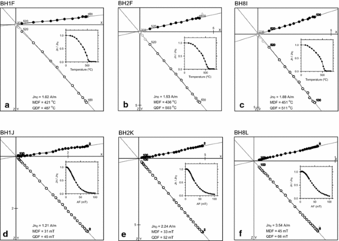
a–c Typical Zijderveld plot for ThD experiments. d–f Typical Zijderveld plot for AFD experiments. Solid circles represent the horizontal projection. Open circles represent the vertical projection. The inserted graph is the stepwise demagnetization curve
Fig. 5 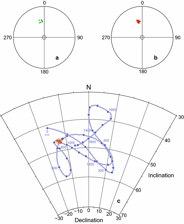
a Direction of the remanent magnetization plotted on the Schmidt net for ThD experiment. b Direction of the remanent magnetization for AFD experiments. c Orange point with orange dashed circle indicates the mean direction with α95 of ThD and AFD experiment. Purple dots represent the reference curve between AD 0 and 2000 at every 50 years proposed by Hirooka (1977)
-
2.
The AFD experiment was conducted for a total of 33 cubic specimens. All the detailed experimental results are shown in Table 4, and typical Zijderveld diagrams are shown in Fig. 4e–g. Like the ThD experimental data, for all samples, the remanence consists primarily of one stable characteristic, remanent magnetization, and the secondary magnetization is very small (the secondary magnetization is almost all demagnetized at 8 mT). The maximum angular deviation (MAD; Kirschvink 1980) values are mostly less than 1°. The median destructive field (MDF) is higher than 30 mT, which indicates that the remanence is very stable and hard (there are specimens with an MDF higher than 70 mT). Equal area projection of the paleodirection is shown in Fig. 5b, and the mean paleodirection is shown in Table 5.
Table 4 Measurement results of the AFD experiment Table 5 Mean direction obtained by the ThD and the AFD experiment


The mean directions in the AFD and ThD experiments coincide within the range of α95 (95% confidence limit). In Fig. 5c, we plot the mean direction of ThD and AFD experiments. In comparison with the reference curve by Hirooka (1977), the mean direction of the remains in this study is plotted close to the paths in (1) AD 500–550 and (2) AD 900–950, within the range of α95. In particular, the mean value overlaps the path in (2) AD 900–950. This age coincides with the archeologically estimated age (AD 900–1000). Therefore, assuming that the reference curve by Hirooka (1977) is accurate, this suggests that the remanent magnetization was acquired at the time of the last burning in AD 900–950.
Archeointensity measurements
The Tsunakawa–Shaw experiment was performed on a total of 8 specimens. All of the specimens yielded results passing the selection criteria, which are listed in Table 6. Typical results are shown in Fig. 6. All the archeointensity values are determined from more than 75% of the total NRMs (f N ≥ 0.75). The slopes of the ARM0–ARM1 diagrams (slopeA0) are almost in unity (0.989–1.07) except for the specimen BH8L, suggesting little influence of laboratory alterations and anisotropies of the remanent magnetizations. The site-mean archeointensity is calculated to be 48.1 μT with a coefficient of variation \(H_{\delta } \%\) of \(6.4\%\) (\(H_{\text{past}} = 48.1 \pm 3.1 \,\upmu{\text{T}}\)) (Table 6).

a, b Typical results of the Tsunakawa–Shaw method. All the samples show similar graph patterned in common (NRM-TRM1 and ARM0-ARM1 ratios show extremely high linearity). The 3 diagrams on the left side show results from the first laboratory heating. The 3 diagrams on the right side show results from the second laboratory heating
The IZZI-Thellier experiments were conducted on a total of 18 specimens. Only the results from 3 specimens passed the selection criteria (success rate is 17%), which are listed in Table 7. The Arai plots of the successful results show excellent linearities (Fig. 7a–c). These results come from samples not showing noticeable dominance of the MD component in the FORC diagram (Fig. 2d). Conversely, the rejected 15 results show nonlinear trends in the Arai plots, such as concave-up curves (Fig. 7d), systematic failures of the pTRM checks with increasing temperatures (Fig. 7e), and zig-zagging behavior (Fig. 7f). These results come from samples both showing and not showing noticeable dominance of the MD component in the FORC diagram (Fig. 2d, e). It is likely that these nonlinearities are due to the alteration of the specimens and/or the effect of MD particles. The site-mean archeointensity is calculated to be 45.3 μT with a coefficient of variation \(H_{\delta } \%\) of \(9.7\%\) (\(H_{\text{past}} = 45.3 \pm 4.4 \,\upmu{\text{T}}\)) (Table 7).

Typical examples of Arai plots of the IZZI-Thellier method of the accepted specimens (a–c) and the rejected specimens (d–f). Solid circles represent the general NRM/TRM ratios. Open triangles represent the points of pTRM check. Green lines indicate the selected straight segment. Red circles (blue circles) correspond to ZI steps (IZ steps)
Discussion
In this study, we applied the two different modern paleointensity methods to the baked clay samples taken from the kiln floor of a Japanese Sueki old kiln. The site-mean archeointensity values resulted in \(48.1 \pm 3.1 \,\upmu{\text{T}} \left( {n = 8} \right)\) by the Tsunakawa–Shaw method and \(45.3 \pm 4.4 \,\,\upmu{\text{T}} \left( {n = 3} \right)\) by the IZZI-Thellier method. The two means are indistinguishable at the 1σ level, with very small coefficients of variation (Fig. 8a), which indicates that they are reliable archeointensity estimates. It is considered that the Tsunakawa–Shaw method can be employed to recover archeointensities with a high reliability and high success rate from archeological relics.

a Comparison of the paleointensity value between the different experimental methods (on the specimen level). Red circles are the values by the IZZI-Thellier method, and the red dashed line is their mean intensity. Green circles are the values by the Tsunakawa–Shaw method, and the green dashed line is their mean intensity. b Paleointensity values (site mean) of this study and previous studies. Green circle is the mean intensity by the Tsunakawa–Shaw method. Red circle is the mean intensity by the IZZI-Thellier method. Gray circles are the mean value reported by the previous studies in Japan extracted from the GROMAGIA 50 database. The errors are standard deviations (1σ)
The reliability of the archeointensity estimates is also ensured from the viewpoint of rock magnetism and mineralogy. The rock magnetic and mineralogical results indicate that the samples are suitable for paleointensity experiments: (1) PSD-like magnetic particle assemblage; (2) little magnetic interaction; (3) single ChRM components; (4) NRMs of TRM origins; (5) continuous blocking temperature distribution; (6) little laboratory alteration; (7) (titano-)magnetite as the main magnetic minerals; and (8) crystallization temperatures as high as 1000 °C for the constituting minerals. All these characters fulfill nearly, although not perfectly, the conditions of “the ideal behavior on the paleointensity experiments” first suggested by Coe (1967) as (1) the additivity law of pTRM, (2) independence law of pTRM, and (3) proportion law of TRM.
To compare our data with previously published data, we extracted the site-mean archeointensity data from the GEOMAGIA 50 database (Korhonen et al. 2008; Brown et al. 2015) by applying site-level selection criteria: a minimum of three successful results for a site (\(n\) \(\ge 3\)) and successful results providing a site mean with a standard deviation less than 20% of the mean (coefficient of variation, \(H_{\delta } \%\) ≤ 20%). It is noted that our data obviously fulfill these criteria. In the GEOMAGIA 50 database, there are two archeointensity results from archeological artifacts in Japan for AD 900–1000: (1) \(58.9 \pm 5.9 \,\upmu{\text{T}}\) at site K-14 of Sasajima (1965) (baked earth, original Thellier method) and (2) \(55.1 \pm 3.7 \upmu{\text{T}}\) of Sakai and Hirooka (1986) (ceramic, Sakai–Thellier method). Regarding data (1), its age was registered as AD \(1000 \pm 20\) (originally reported in Sasajima 1965) but was corrected to AD \(960 \pm 20\) in Sasajima and Maenaka (1966). We adopted the corrected age value for the data (1; Fig. 8b). Furthermore, the age as AD \(1120 \pm 20\) of (3) \(58.2 \pm 1.2\,\,\upmu{\text{T}}\) at site O-53 (baked earth, original Thellier method) in Sasajima (1965) was corrected to AD \(1000 \pm 20\) in Sasajima and Maenaka (1966). Therefore, we also added the site-mean intensity value in this article (Fig. 8b). All of them were significantly higher than the results obtained by this study at the 1σ level (Fig. 8b).
One of the possible causes is thought to be undetected laboratory alterations in the previous study data because they were yielded by Thellier-type methods without pTRM checks. Another possible cause is that the linear segments in Arai plots might be selected in a biased way from low blocking temperature portions constituting a part of concave-up curves in previous studies. In recent studies, such Arai plots are interpreted to be affected by MD particles, and therefore, the intensity values calculated from such plots should be rejected because the reliability is suspicious (Tauxe 2010; Paterson 2011; Tanaka and Yamamoto 2016). Among the three previous data, Arai plots from sites K-14 and O-53 are, respectively, presented in Sasajima (1965) and Sasajima and Maenaka (1966). The Arai plot of site K-14 shows a straight line between room temperature and 500 °C, but some portion of NRM remains for a temperature range higher than 500 °C and is not associated with the pTRM check: the plot might be potentially convex downward. The two Arai plots of site O-53 are linear throughout all temperature ranges, but they were not associated with the pTRM checks.
Published site-mean archeointensity results in Japan selected from the GEOMAGIA 50 database for the last 2 kyr (Nagata et al. 1963; Sasajima 1965; Sasajima and Maenaka 1966; Sakai and Hirooka 1986) are all higher than the archeointensities obtained by the present study (Fig. 8b). They are mostly from Sakai and Hirooka (1986), and some of the Arai plots presented in their paper appear to be convex downward. It is speculated that they might systematically overestimate the past variation of the geomagnetic field intensity around Japan at the time.
Conclusion
In this study, we tested the suitability of the Tsunakawa–Shaw paleointensity method for analyzing baked clay samples collected from the floor of the Sayama Higashiyama-Oku kiln by comparing the results with those collated using the IZZI-Thellier method.
The intensity from the Tsunakawa–Shaw method was 48.1 ± 3.1 μT (N = 8) and that from the IZZI-Thellier method was 45.3 ± 4.4 μT (N = 3). The results from both methods coincide within the range of their standard deviations (1σ). Therefore, these experimental results suggest that the Tsunakawa–Shaw method is suitable for reconstructing paleointensity values from real archeological materials with high reliability.
From rock magnetic experiments, mineral analysis, and paleodirection measurements, it was revealed that the main magnetic mineral in the samples is titanomagnetite, the alteration during heating is very small, and the recorded NRM is the only single component of TRM acquired in the operating time at temperatures greater than 1000 °C. Thus, we confirmed that the samples used in this study are suitable for paleointensity experiments.
The two intensity values from the modern experimental methods are lower than those from previous studies in Japan.
References
Ahn HS, Kidane T, Yamamoto Y, Otofuji YI (2016) Low geomagnetic field intensity in the Matuyama Chron: palaeomagnetic study of a lava sequence from Afar depression, East Africa. Geophys J Int 204:127–146. https://doi.org/10.1093/gji/ggv303
Arai T (1963) Secular variation in the intensity of the past geomagnetic field. M.Sc. Thesis, University of Tokyo
As JA, Zijderveld JDA (1958) Magnetic cleaning of rocks in paleomagnetic research. Geophys J 1:308–319
Berna F, Behar A, Shahack-Gross R, Berg J, Boaretto E, Gilboa A, Sharon I, Shalev S, Shilstein S, Yahalom-Mack N, Zorn JR, Weiner S (2007) Sediments exposed to high temperatures: reconstructing pyrotechnological processes in Late Bronze and Iron Age Strata at Tel Dor (Israel). J Archaeol Sci 34:358–373. https://doi.org/10.1016/j.jas.2006.05.011
Brown MC, Donadini F, Korte M, Nilsson A, Korhonen K, Lodge A, Lengyel SN, Constable CG (2015) GEOMAGIA50.v3: 1. General structure and modifications to the archeological and volcanic database. Earth Planets Space. https://doi.org/10.1186/s40623-015-0232-0
Cai S, Tauxe L, Deng C, Pan Y, Jin G, Zheng J, Xie F, Qin H, Zhu R (2014) Geomagnetic intensity variations for the past 8 kyr: new archaeointensity results from Eastern China. Earth Planet Sci Lett 392:217–229. https://doi.org/10.1016/j.epsl.2014.02.030
Cai S, Chen W, Tauxe L, Deng C, Qin H, Pan Y, Zhu R (2015) New constraints on the variation of the geomagnetic field during the late Neolithic period: archaeointensity results from Sichuan, southwestern China. J Geophys Res 120:2056–2069
Cai S, Jin G, Tauxe L, Deng C, Qin H, Pan Y, Zhu R (2017) Archaeointensity results spanning the past 6 kiloyears from eastern China and implications for extreme behaviors of the geomagnetic field. Proc Natl Acad Sci 114:39–44. https://doi.org/10.1073/pnas.1616976114
Coe RS (1967) Paleo-intensities of the Earth’s magnetic field determined from tertiary and quaternary rocks. J Geophys Res 72:3247–3262
Coe RS, Grommé S, Mankinen EA (1978) Geomagnetic paleointensities from radiocarbon-dated lava flows on Hawaii and the question of the Pacific nondipole low. J Geophys Res 83:1740–1756. https://doi.org/10.1029/JB083iB04p01740
Cromwell G, Tauxe L, Staudigel H, Ron H (2015) Paleointensity estimates from historic and modern Hawaiian lava flows using glassy basalt as a primary source material. Phys Earth Planet Inter 241:44–56. https://doi.org/10.1016/j.pepi.2014.12.007
Day RM, Fuller M, Schmidt VA (1977) Hysteresis properties of titanomagnetites: grain-size and compositional dependence. Phys Earth Planet Inter 13:260–267
Doi A, Sakamoto N (2002) Baking process of Bizen-yaki pottery. In: Okayama University of Science (ed) Research group for “Okayamaology”. Scientific Research of Bizen-Yaki Pottery. “Okayamaology,” vol 1, Kibito Shuppan, Okayama, pp 38–45 (in Japanese)
Domen H (1977) A single heating method of paleomagnetic field intensity determination applied to old roof tiles and rocks. Phys Earth Planet Inter 13:315–318. https://doi.org/10.1016/0031-9201(77)90115-7
Doubrovine PV, Tarduno JA (2006) N-type magnetism at cryogenic temperatures in oceanic basalt. Phys Earth Planet Inter 157:46–54. https://doi.org/10.1016/j.pepi.2006.03.002
Egli R, Chen AP, Winklhofer M, Kodama KP, Horng CS (2010) Detection of noninteracting single domain particles using first-order reversal curve diagrams. Geochem Geophys Geosyst. https://doi.org/10.1029/2009GC002916
Hatakeyama T, Kitahara Y, Tamai Y, Torii M (2014) Chapter 6: Scientific analysis 2 –Paleomagnetic study for 3 old kilns of Sayama area in Bizen city, Okayama–. In: Archeology Laboratory of Faculty of Biosphere-Geosphere Science, Okayama University of Science (ed) Study of Bizen Oku kiln complex –Study on ancient ceramic production–. Archeology Laboratory of Faculty of Biosphere-Geosphere Science, Okayama University of Science, Okayama, pp 85–105 (in Japanese)
Heider F, Dunlop DJ, Soffel HC (1992) Low-temperature and alternating field demagnetization of saturation remanence and thermoremanence in magnetite grains (0.037 μm to 5 mm). J Geophys Res 97:9371–9381
Heslop D, Dekkers MJ, Kruiver PP, van Oorschot IHM (2002) Analysis of isothermal remanent magnetization acquisition curves using the expectation-maximization algorithm. Geophys J Int 148:58–64. https://doi.org/10.1046/j.0956-540x.2001.01558.x
Hirooka K (1977) Recent trends in archaeomagnetic and palaeomagnetic studies in quaternary research. Daiyonki Kenkyu 15:200–203 (in Japanese with English abstract)
Hong H, Yu Y, Lee CH, Kim RH, Park J, Doh SJ, Kim W, Sung H (2013) Globally strong geomagnetic field intensity circa 3000 years ago. Earth Planet Sci Lett 383:142–152. https://doi.org/10.1016/j.epsl.2013.09.043
International Association of Geomagnetism and Aeronomy, Working Group V-MOD (2010) International geomagnetic reference field: the eleventh generation. Geophys J Int 183:1216–1230. https://doi.org/10.1111/j.1365-246X.2010.04804.x
Itoh A (1987) Chapter XI: Ceramic industry. In: Kondoh Y (ed) Archaeology of Okayama prefecture, 1st edn. Yoshikawa Kobunkan, Tokyo, pp 531–588 (in Japanese)
Jordanova N, Kovacheva M, Kostadinova M (2004) Archaeomagnetic investigation and dating of Neolithic archaeological site (Kovachevo) from Bulgaria. Phys Earth Planet Inter 147:89–102
Kameda S (1996) Chronology of the main old kilns in Sanyo area. In: Funayama R, Matsumoto T, Ikeda Y (eds) Sueki catalog, Western Japan, vol 5, 1st edn. Yuzankaku Inc., Tokyo, p 94 (in Japanese)
Kameda S, Sjiraishi J, Tokusawa K, Imamura K (2014) Chapter 5: Sayama Higashiyama kiln complex 2—Sayama Higashiyama-Oku kiln. In: Archeology Laboratory of Faculty of Biosphere–Geosphere Science, Okayama University of Science (eds) Study of Bizen Oku kiln complex—study on ancient ceramic production. Archeology Laboratory of Faculty of Biosphere-Geosphere Science, Okayama University of Science, Okayama, pp 59–74 (in Japanese)
Kirschvink JL (1980) The least-square line and plane and the analysis of paleomagnetic data. Geophys J R Astron Soc 62:699–718
Kitazawa K (1970) Intensity of the geomagnetic field in Japan for the past 10,000 years. J Geophys Res 75:7403–7411. https://doi.org/10.1029/JB075i035p07403
Korhonen K, Donadini F, Riisager P, Pesonen LJ (2008) GEOMAGIA50: an archeointensity database with PHP and MySQL. Geochem Geophys Geosyst. https://doi.org/10.1029/2007GC001893
Lanos P (2004) Bayesian inference of calibration curves: application to archaeomagnetism. In: Buck CE, Millard AR (eds) Lecture notes in statistics. Tools for constructing chronologies: crossing discipline boundaries. Springer, Berlin, pp 43–82
Mizoguchi K (2013) The archaeology of Japan: From the earliest rice farming villages to the rise of the state. Cambridge University Press, Cambridge, p 371
Mochizuki N, Tsunakawa H, Oishi Y, Wakai S, Wakabayashi KI, Yamamoto Y (2004) Palaeointensity study of the Oshima 1986 lava in Japan: implications for the reliability of the Thellier and LTD-DHT Shaw methods. Phys Earth Planet Inter 146:395–416. https://doi.org/10.1016/j.pepi.2004.02.007
Mochizuki N, Tsunakawa H, Shibuya H, Cassidy J, Smith IE (2006) Palaeointensities of the Auckland geomagnetic excursions by the LTD-DHT Shaw method. Phys Earth Planet Inter 154:168–179
Mochizuki N, Oda H, Ishizuka O, Yamazaki T, Tsunakawa H (2011) Paleointensity variation across the Matuyama–Brunhes polarity transition: observations from lavas at Punaruu Valley, Tahiti. J Geophys Res. https://doi.org/10.1029/2010JB008093
Mochizuki N, Maruuchi T, Yamamoto Y, Shibuya H (2013) Multi-level consistency tests in paleointensity determinations from the welded tuffs of the Aso pyroclastic-flow deposits. Phys Earth Planet Inter 223:40–54. https://doi.org/10.1016/j.pepi.2013.05.001
Nagata T, Akimoto S (1961) Chapter III: magnetic properties of rock-forming ferromagnetic minerals. In: Nagata T (ed) Rock magnetism. Maruzen Co Ltd, Tokyo, pp 75–125
Nagata T, Arai T, Momose K (1963) Secular variation of the geomagnetic total force during the last 5000 years. J Geophys Res 68:5277–5281
Nagayama U (1936) History of Kibi-gun. Educational Society of Kibi-gun, Okayama (in Japanese)
Nakajima T, Natsuhara N (1981) Archaeomagnetic dating method. Archaeological library, no 9. New Science Co., Tokyo, p 95 (in Japanese)
National Institute of Advanced Industrial Science and Technology (2017) 1/200,000 Seamless geological map of Japan. gbank.gsj.jp/seamless/2d3d/?center=34.6938, 134.1903&z=13. Accessed 22 Dec 2017 (in Japanese)
Nishikawa H (1966) Chronological study of Sueki in Bizen. Report of the private education in Okayama prefecture (in Japanese)
Oishi Y, Tsunakawa H, Mochizuki N, Yamamoto Y, Wakabayashi KI, Shibuya H (2005) Validity of the LTD-DHT Shaw and Thellier palaeointensity methods: a case study of the Kilauea 1970 lava. Phys Earth Planet Inter 149:243–257. https://doi.org/10.1016/j.pepi.2004.10.009
Ozima M, Ozima M, Akimoto S (1964) Low temperature characteristics of remanent magnetization of magnetite—self-reversal and recovery phenomena of remanent magnetization. J Geomagn Geoelectr 16:165–177
Paterson GA (2011) A simple test for the presence of multidomain behavior during paleointensity experiments. J Geophys Res. https://doi.org/10.1029/2011JB008369
Petschick R (2000) MacDiff Ver. 4.2.3, Manual. Geologisch-Paläontrologisches Institut Johann Wolfgang-Universität Frankfurt am Main Senckenberganlage, Frankfurt am Main
Sakai H, Hirooka K (1986) Archaeointensity determinations from Western Japan. J Geomagn Geoelectr 38:1323–1329
Sasajima S (1965) Geomagnetic secular variation revealed in the baked earths in West Japan (part 2) change of the field intensity. J Geomagn Geoelectr 17:413–416. https://doi.org/10.5636/jgg.17.413
Sasajima S, Maenaka K (1966) Intensity studies of the archaeo-secular variation in West Japan, with special reference to the hypothesis of the dipole axis rotation. Mem Coll Sci Kyoto Univ Ser B 33:53–67
Schomburg J (1991) Thermal reactions of clay minerals: their significance as “archaeological thermometers” in ancient potteries. Appl Clay Sci 6:215–220. https://doi.org/10.1016/0169-1317(91)90026-6
Shaar R, Tauxe L (2013) Thellier GUI: an integrated tool for analyzing paleointensity data from Thellier-type experiments. Geochem Geophys Geosyst 14:677–692. https://doi.org/10.1002/ggge.20062
Shiraishi J, Kyoguro S (2002) Distribution of a Bizen-yaki mortar revealed by scientific investigation. In: Research group for “Okayamaology”, Okayama University of Science (eds) Scientific research of Bizen-yaki pottery. “Okayamaology,” vol 1. Kibito Shuppan, Okayama, pp 62–71 (in Japanese)
Tanaka H, Kobayashi T (2003) Paleomagnetism of the late Quaternary Ontake Volcano, Japan: directions, intensities, and excursions. Earth Planets Space 55:189–202. https://doi.org/10.1186/BF03351748
Tanaka H, Yamamoto Y (2016) Palaeointensities from Pliocene lava sequences in Iceland: emphasis on the problem of Arai plot with two linear segments. Geophys J Int 205:694–714. https://doi.org/10.1093/gji/ggw031
Tauxe L (2010) Essentials of paleomagnetism. University of California Press, California
Tauxe L, Staudigel H (2004) Strength of the geomagnetic field in the cretaceous normal superchron: new data from submarine basaltic glass of the troodos ophiolite. Geochem Geophys Geosyst. https://doi.org/10.1029/2003GC000635
Tauxe L, Mullender TAT, Pick T (1996) Potbellies, wasp-waists, and superparamagnetism in magnetic hysteresis. J Geophys Res 101:571–583
Thellier E, Thellier O (1959) Sur l’intensité du champ magnétique terrestre Dans le passé historique et géologique. Ann Géophys 15:285–376 (in French with English abstract)
Winklhofer M, Zimanyi GT (2006) Extracting the intrinsic switching field distribution in perpendicular media: a comparative analysis. J Appl Phys 99:08E710. https://doi.org/10.1063/1.2176598
Yamamoto Y, Tsunakawa H (2005) Geomagnetic field intensity during the last 5 Myr: LTD-DHT Shaw palaeointensities from volcanic rocks of the Society Islands, French Polynesia. Geophys J Int 162:79–114
Yamamoto Y, Tsunakawa H, Shibuya H (2003) Palaeointensity study of the Hawaiian 1960 lava: Implications for possible causes of erroneously high intensities. Geophys J Int. https://doi.org/10.1046/j.1365-246x.2003.01909.x
Yamamoto Y, Shibuya H, Tanaka H, Hoshizumi H (2010) Geomagnetic paleointensity deduced for the last 300 kyr from Unzen Volcano, Japan, and the dipolar nature of the Iceland Basin excursion. Earth Planet Sci Lett 293:236–249. https://doi.org/10.1016/j.epsl.2010.02.024
Yamamoto Y, Torii M, Natsuhara N (2015) Archeointensity study on baked clay samples taken from the reconstructed ancient kiln: implication for validity of the Tsunakawa–Shaw paleointensity method. Earth Planets Space. https://doi.org/10.1186/s40623-015-0229-8
Yamazaki T, Yamamoto Y (2014) Paleointensity of the geomagnetic field in the Late Cretaceous and earliest Paleogene obtained from drill cores of the Louisville seamount trail. Geochem Geophys Geosyst 15:2454–2466. https://doi.org/10.1002/2014GC005298
Yu Y (2012) High-fidelity paleointensity determination from historic volcanoes in Japan. J Geophys Res. https://doi.org/10.1029/2012JB009368
Authors’ contributions
YK carried out sampling, paleointensity experiments, mineralogical measurements, and a part of the rock magnetic measurements, supervised by YY and MO. Y Kuwahara supervised Y Kitahara in the mineralogical measurements. SK led the archeological study and determined the age of the kiln. TH conducted the paleodirection and a part of the rock magnetic measurements. All authors contributed to the discussion, and YK wrote the manuscript. All authors read and approved the manuscript.
Acknowledgements
We thank Jun Shiraishi, Keiichi Tokusawa, and Satoshi Yokoyama for help with the sampling at the archeological site, Shinsuke Yagyu and Chisa Nishimori for help with the archeointensity experiments, Lisa Tauxe for help with the paleointensity analysis, Hiroto Fukami for help with the rock magnetic measurements, Masato Makio for help with the mineralogical measurements, and Hironobu Kan for letting us use the rock cutter. Constructive comments were received from Hidetoshi Shibuya, Hideo Tsunakawa, Futoshi Takahashi, Masahiko Sato, and Ryo Hemmi. In addition, we thank guest lead editor John Tarduno, reviewer Nobutatsu Mochizuki, and another anonymous reviewer for their useful and suggestive comments. This study was partly conducted under the cooperative research program of the Center for Advanced Marine Core Research (CMCR), Kochi University (Accept 12B028, 13A027, 15A006, 15B006, 15B060, 16A034, 16A046, 16B030, 16B073, 17A031, 17A033, 17B031, and 17B033). The study was partly supported by JSPS KAKENHI Grant Number JP16H01826.
Competing interests
The authors declare that they have no competing interests.
Availability of data and materials
The data and materials used in this study are available on request from the corresponding author, Yu Kitahara (3gs15005w@s.kyushu-u.ac.jp).
Ethics approval and consent to participate
Not applicable.
Funding
This study was partly funded by JSPS KAKENHI Grant Number JP16H01826.
Publisher’s Note
Springer Nature remains neutral with regard to jurisdictional claims in published maps and institutional affiliations.
Author information
Authors and Affiliations
Corresponding author
Rights and permissions
Open Access This article is distributed under the terms of the Creative Commons Attribution 4.0 International License (http://creativecommons.org/licenses/by/4.0/), which permits unrestricted use, distribution, and reproduction in any medium, provided you give appropriate credit to the original author(s) and the source, provide a link to the Creative Commons license, and indicate if changes were made.
About this article

Cite this article
Kitahara, Y., Yamamoto, Y., Ohno, M. et al. Archeointensity estimates of a tenth-century kiln: first application of the Tsunakawa–Shaw paleointensity method to archeological relics. Earth Planets Space 70, 79 (2018). https://doi.org/10.1186/s40623-018-0841-5
Received:
Accepted:
Published:
DOI: https://doi.org/10.1186/s40623-018-0841-5