
Abstract
In this study, we investigate the global exponential stability of Clifford-valued neural network (NN) models with impulsive effects and time-varying delays. By taking impulsive effects into consideration, we firstly establish a Clifford-valued NN model with time-varying delays. The considered model encompasses real-valued, complex-valued, and quaternion-valued NNs as special cases. In order to avoid the issue of non-commutativity of the multiplication of Clifford numbers, we divide the original n-dimensional Clifford-valued model into \(2^{m}n\)-dimensional real-valued models. Then we adopt the Lyapunov–Krasovskii functional and linear matrix inequality techniques to formulate new sufficient conditions pertaining to the global exponential stability of the considered NN model. Through numerical simulation, we show the applicability of the results, along with the associated analysis and discussion.
1 Introduction
Dynamic analysis of neural network (NN) models has gained tremendous research interest in recent decades, since NN models play a significant role in various applications. In particular, the stability theory of NN models has been extensively studied to solve many problems related to science and engineering, including associative memory, image and signal processing, optimization, pattern recognition and others [1–8]. On the other hand, complex signals exist in most NN applications in the real world. As such, multidimensional problems such as color night vision, radar imaging, polarized signal classification, 3D wind forecasting can be solved more favorably by implementing complex-valued and quaternion-valued NN models [9–26]. To date, several important results regarding various dynamics of complex-valued and quaternion-valued NN models have been published, some of them stability analysis [13, 14, 20–22, 26], synchronization analysis [11], stabilizability and instabilizability [12], controllability and observability [23], optimization [24, 25] and so on.
Clifford algebra offers a powerful framework for solving geometrical problems. This discipline has shown useful results in various science and engineering areas, including control and robotic related problems [27–31]. Clifford-valued NN models stand as a generalization of real-valued, complex-valued, and quaternion-valued NNs. In this respect, Clifford-valued NN models are superior to real-valued, complex-valued, and quaternion-valued NNs for undertaking spatial geometric transformation and high-dimensional data problems [29–32]. Theoretical and applied studies of Clifford-valued NN models have recently become a new topic of research. However, the dynamical properties of Clifford-valued NN models are typically more complex than those of real-valued and complex-valued NN models. As such, studies on Clifford-valued NN dynamics are still limited due to those utilizing the principle of non-commutativity of the product of Clifford numbers [33–42].
In [33], the authors derived the global exponential stability criteria for delayed Clifford-valued recurrent NN models in terms of linear matrix inequalities (LMIs). Pertaining to Clifford-valued NN models with time delays, their global asymptotic stability issues were examined in [34] by decomposing the n-dimensional Clifford-valued NN model into \(2^{m}n\)-dimensional real-valued models. Leveraging on a direct method, the existence and global exponential stability of almost periodic solutions were derived for Clifford-valued neutral high-order Hopfield NN models with leakage delays in [37]. In addition, the use of Banach fixed point theorem and Lyapunov–Krasovskii functional (LKF) technique for addressing the global asymptotic almost periodic synchronization issues for Clifford-valued cellular NN models was conducted in [38]. A study of the weighted pseudo almost automorphic solutions pertaining to neutral type fuzzy cellular NN models with mixed delays and D operator in Clifford algebra was presented in [40]. In [42], the authors investigated the existence of anti-periodic solutions corresponding to a class of Clifford-valued inertial Cohen–Grossberg NN models by constructing suitable LKFs.
Due to the limited speed of signal propagation, time delays (either constant or time-varying) are often encountered in NN models operating in real-world applications [3, 5–8]. Time delays are the main source of various dynamics such as chaos, divergence, poor functionality and instability [11–13, 36, 39, 41]. Hence it is necessary to analyze the NN dynamics that incorporate either constant or time-varying delays. In this respect, NN models with various time delays have been extensively studied, and many significant results have been obtained [3, 5, 11–13, 33–46]. On the other hand, due to noise, change in frequency, or switching phenomenon, the impulsive effects occur in real-world systems [47]. The resulting dynamical behaviors of the systems are more complex than those of classical dynamical systems [47, 48]. Generally, impulses can affect the dynamic behaviors of networks. As such, many papers dealing with dynamical systems with impulsive effects have appeared in recent years [43–50].
To the best of our knowledge, there are hardly any papers that deal with the issue of global exponential stability of Clifford-valued NNs with time-varying delays and impulsive effects. Indeed, this interesting subject remains an open challenge. Motivated by the above facts, our research focuses on to derive the sufficient conditions of global exponential stability of Clifford-valued NNs with impulsive effects. In order to achieve our main results, the n-dimensional Clifford-valued NN model is firstly decomposed into \(2^{m}n\)-dimensional real-valued NN models. This avoids the issues related to the principle of non-commutativity of multiplication with respect to Clifford numbers. Based on the LKF and LMI techniques and some mathematical concepts, we derive new sufficient conditions for ascertaining the exponential stability of the considered Clifford-valued NN model. The conditions obtained in this study are expressed in LMIs, and the associated feasible solutions are verified by using the MATLAB software. The obtained results are validated with a numerical simulation.
The main contributions of our study are as follows: (1) we for the first time analyze the global exponential stability of Clifford-valued NN models with time-varying delays as well as impulsive effects; (2) in comparison with other results, the results of our study is new and more general even when the considered Clifford-valued NN model has been decomposed into real-, complex-, and quaternion-valued NN models; (3) our proposed method can be easily employed for other dynamic behaviors with respect to different types of Clifford-valued NN models.
The organization of this article is as follows. The proposed Clifford-valued NN model is formally defined in Sect. 2. We then explain the new stability criterion and present the numerical example and the associated simulation results in Sects. 3 and 4, respectively. A summary of the findings is given in Sect. 5.
2 Mathematical Fundamentals and Problem Formulation
2.1 Notations
Let \(\mathbb{R}^{n}\) and \(\mathbb{A}^{n}\) denote the n-dim real vector space and n-dim real Clifford vector space, respectively. \(\mathbb{R}^{n \times n}\) and \(\mathbb{A}^{n \times n}\) denote the set of all \(n \times n\) real matrices and the set of all \(n \times n\) real Clifford matrices, respectively. \(\mathbb{A}\) is defined as the Clifford algebra with m generators over the real number \(\mathbb{R}\). Superscripts T and ∗, respectively, indicate matrix transposition and matrix involution transposition. A matrix  (<0) denotes a positive (negative) definite matrix. We define the norm of \(\mathbb{R}^{n}\) as \(\|p\|=\sum_{i=1}^{n}|p_{i}|\). Besides that,
  , denote \(\|B\|=\max_{1\leq i\leq n}\{\sum_{j=1}^{n}|b_{ij}| \}\), while \(p=\sum_{A}p^{A}e_{A}\in \mathbb{A}\) denote \(\|p\|_{\mathbb{A}}=\sum_{A}|p^{A}|\) and for
  , denote \(\|B\|_{\mathbb{A}}=\max_{1\leq i\leq n}\{\sum_{j=1}^{n}|b_{ij}|_{ \mathbb{A}}\}\). For \(\varphi \in \mathcal{C}([-\tau , 0], \mathbb{A}^{n})\), we introduce the norm \(\|\varphi \|_{\tau }\leq \sup_{-\tau \leq s\leq 0}\|\varphi (t+s) \|\).
  and
and  , respectively, denote the maximum and minimum eigenvalues of matrix
  .
.
2.2 Clifford Algebra
The Clifford real algebra over \(\mathbb{R}^{m}\) is defined as
where \(e_{A}=e_{h_{1}}e_{h_{2}}\ldots e_{h_{\nu }}\) with \(A=\{h_{1},h_{2},\ldots ,h_{\nu }\}\), \(1 \leq h_{1} < h_{2} <\cdots < h_{\nu }\leq m\).
Moreover \(e_{\emptyset }=e_{0}=1\) and \(e_{h}=e_{\{h\}}\), \(h=1,2,\ldots ,m\) are denoted as the Clifford generators, and they fulfill the following relationship:
For the sake of simplicity, when an element is the product of multiple Clifford generators, its subscripts are incorporated together, e.g. \(e_{4}e_{5}e_{6}e_{7}=e_{4567}\).
Let \(\Lambda =\{\emptyset ,1,2,\ldots , A,\ldots , 12\dots m\}\), and we have
where \(\sum_{A}\) denotes \(\sum_{A\in \Lambda }\) and \(\mathbb{A}\) is isomorphic to \(\mathbb{R}^{2^{m}}\).
For any Clifford number \(p=\sum_{A}p^{A}e_{A}\), the involution of p is defined by
where \(\bar{e}_{A}=(-1)^{\frac{\sigma [A](\sigma [A]+1)}{2}}e_{A}\), and
From the definition, we can directly deduce that \(e_{A}\bar{e}_{A}=\bar{e}_{A}e_{A}=1\). For a Clifford-valued function \(p=\sum_{A}p^{A}e_{A}:\mathbb{R}\rightarrow \mathbb{A}\), where \(p^{A}:\mathbb{R}\rightarrow \mathbb{R}\), \(A\in \Lambda \), and its derivative is represented by \(\frac{dp(t)}{dt}=\sum_{A}\frac{dp^{A}(t)}{dt}e_{A}\).
Since \(e_{B}\bar{e}_{A}=(-1)^{\frac{\sigma [A](\sigma [A]+1)}{2}}e_{B}e_{A}\), we can write \(e_{B}\bar{e}_{A}=e_{C}\) or \(e_{B}\bar{e}_{A}=-e_{C}\), where \(e_{C}\) is a basis of Clifford algebra \(\mathbb{A}\). As an example, \(e_{h_{1}h_{2}}\bar{e}_{h_{2}h_{3}}=-e_{h_{1}h_{2}}e_{h_{2}h_{3}} =-e_{h_{1}}e_{h_{2}}e_{h_{2}}e_{h_{3}}=-e_{h_{1}}(-1)e_{h_{3}}=e_{h_{1}}e_{h_{3}} = e_{h_{1}h_{3}}\). Therefore, it is possible to identify a unique corresponding basis \(e_{C}\) for a given \(e_{B}\bar{e}_{A}\). Define
and then \(e_{B}\bar{e}_{A} =(-1)^{\sigma [B.\bar{A}]}e_{C}\).
Moreover, for any \(\mathscr{G}\in \mathbb{A}\), there is a unique \(\mathscr{G}^{C}\) that satisfies \(\mathscr{G}^{B.\bar{A}}=(-1)^{\sigma [B.\bar{A}]}\mathscr{G}^{C}\) for \(e_{B}\bar{e}_{A}=(-1)^{\sigma [B.\bar{A}]}e_{C}\). Therefore
and \(\mathscr{G}= \sum_{C}\mathscr{G}^{C}e_{C} \in \mathbb{A}\).
2.3 Problem Definition
Consider a Clifford-valued NN model with time-varying delays, as follows:
where \(i,j= 1,2,\ldots ,n\), and n corresponds to the number of neurons; \(p_{i}(t)\in \mathbb{A}\) represents the state vector of the ith unit; \(d_{i}\in \mathbb{R}^{+}\) indicates the rate with which the ith unit resets its potential to the resting state in isolation when it is disconnected from the network and external inputs; \(a_{ij}, b_{ij}\in \mathbb{A}\) indicate the strengths of connection weights without and with time-varying delays between cells i and j, respectively; \(u_{i}\in \mathbb{A}\) is an external input of the ith unit; \(g_{j}(\cdot ):\mathbb{A}^{n} \rightarrow \mathbb{A}^{n}\) is the activation functions of signal transmission; \(\tau (t)\in \mathbb{R}^{+}\) is the transmission delay at time t. Furthermore, \(\varphi _{i}\in \mathcal{C}([-\tau , 0],\mathbb{A}^{n})\) is the initial condition for the considered NN model (1).
The impulsive Clifford-valued NN model with time-varying delays can be described as follows:
where \(\triangle p_{i}(t_{k})= p_{i}(t_{k}^{+})-p_{i}(t_{k}^{-})\) is the jump in state variable \(p_{i}\). In addition, the impulsive moment \(t_{k}\) (\(k\in \mathbb{N}\)) fulfills \(0< t_{1}< t_{2}<\cdots t_{k}<\cdots \) , which is a strictly increasing sequence such that \(\lim_{k\rightarrow +\infty }t_{k}=+\infty \); \(p_{i}(t_{k}^{+})\) and \(p_{i}(t_{k}^{-})\) are the right and left limits of \(p_{i}(t_{k})\), respectively, while \(I_{ik}\in \mathcal{C}[\mathbb{R}^{n}, \mathbb{R}^{n}]\) denotes the incremental change of the state at time \(t_{k}\), while \(I_{ik}(0)=0\) for all \(k\in \mathbb{N}\).
For the convenience of discussion, we rewrite (2) in the vector form

where \(p(t)=(p_{1}(t),p_{2}(t),\ldots,p_{n}(t))^{T}\in \mathbb{A}^{n}\);  with \(d_{i}>0\), \(i=1,2,\ldots,n\); and
  ;
;  ; \(u=(u_{1},u_{2},\ldots,u_{n})^{T}\in \mathbb{A}^{n}\); \(g(p(t))=(g_{1}(p_{1}(t)),g_{2}(p_{2}(t)),\ldots,g_{n}(p_{n}(t)))^{T} \in \mathbb{A}^{n}\); \(g(p(t-\tau (t)))=(g_{1}(p_{1}(t-\tau (t))),g_{2}(p_{2}(t-\tau (t))),\ldots,g_{n}(p_{n}(t- \tau (t))))^{T}\in \mathbb{A}^{n}\) and
  .
.
(H1) Function \(g_{j}(\cdot )\) fulfills the Lipschitz continuity condition with respect to the n-dimensional Clifford vector. For each \(j=1,2,\ldots,n\), there exists a positive constant \(k_{j}\) such that, for any \(x, y\in \mathbb{A}\),
where \(k_{j}\) is known as the Lipschitz constant and \(g_{j}(0)=0\). And there exist positive constants \(k_{j}\) such that \(|g_{j}(x)|_{\mathbb{A}}\leq k_{j}\) (\(j=1,2,\ldots,n\)).
Remark 2.1
There exists a constant \(k_{j}>0\) (\(j=1,2,\ldots,n\)) such that \(\forall x=(x_{1}, x_{2},\ldots, x_{2^{m}})^{T}\in \mathbb{R}^{2^{m}}\), and \(\forall y=(y_{1}, y_{2},\ldots, y_{2^{m}})^{T}\in \mathbb{R}^{2^{m}}\)
By means of assumption (H1), it is clear that

where  .
.
(H2) Time-varying delay \(\tau (t)\) is differential and it fulfills the following conditions:
where τ and μ are known real constants.
Remark 2.2
It is worth noting that Clifford-valued NN models are the generalized form of real-, complex-, and quaternion-valued NN models. For example, when we take into account \(m=0\) in NN model (3), then the model can be reduced to the real-valued NN model proposed in [6]. Suppose, we take \(m=1\) in NN model (3), then the model can be reduced to the complex-valued NN model proposed in [14]. If we choose \(m=2\) in NN model, then the model can be reduced to the quaternion-valued NN model proposed in [26]. Therefore, the proposed system model in this paper is more general than the system model proposed in [6, 14, 26].
Definition 2.3
([34])
With reference to the Clifford-valued NN model (3), the vector \(p^{*}=(p_{1}^{*},p_{2}^{*},\ldots,p_{n}^{*})^{T}\in \mathbb{A}^{n}\) is an equilibrium point, if and only if \(p^{*}\) is a solution of the following equation:

and the impulsive jump  is able to satisfy
  , \(k\in \mathbb{N}\).
Definition 2.4
([39])
Pertinent to the Clifford-valued NN model (3), its global exponential stable is guaranteed if for any solution \(p(t, t_{0},\varphi )\) with the initial condition \(\varphi \in \mathcal{C}([-\tau , 0], \mathbb{A}^{n})\), there exist constants \(\alpha >0\) and  such that

3 Main results
In order to avoid the issues of non-commutativity of multiplication of Clifford numbers, we transform the Clifford-valued NN model (3) into the real-valued NN models. This can be achieved with the help of \(e_{A}\bar{e}_{A}=\bar{e}_{A}e_{A}=1\) and \(e_{B}\bar{e}_{A}e_{A}=e_{B}\). Given any \(\mathscr{G}\in \mathbb{A}\), a unique \(\mathscr{G}^{C}\) that is able to satisfy \(\mathscr{G}^{C}e_{C}g^{A}e_{A}=(-1)^{\sigma [B.\bar{A}]}\mathscr{G}^{C}g^{A}e_{B}= \mathscr{G}^{B.\bar{A}}g^{A}e_{B}\) can be identified. By decomposing (3) into \(\dot{p}=\sum_{A}\dot{p}^{A}e_{A}\), we have

where

Corresponding to the basis of Clifford algebra, we reformulate the Clifford-valued NN model to novel real-valued ones. Define

The NN model (8) can be written as

with the initial value
where \(\bar{\varphi }(s)=((\varphi ^{0}(s))^{T},(\varphi ^{1}(s))^{T},\ldots,( \varphi ^{A}(s))^{T},\ldots,(\varphi ^{12\ldots m}(s))^{T})^{T}\in \mathbb{R}^{2^{m}n}\).
In addition, we can express (6) as the following inequality:

where

From Definition 2.3 there exists a unique equilibrium point \(w^{*}\) for Clifford-valued NN model (9). Next, we prove the global exponential stability of (9). Firstly, we shift the equilibrium point of (9) to the origin using the transformation \(\tilde{w}=w-w^{*}\). Then we rewrite Clifford-valued NN model (9) as

where \(\tilde{g}(\tilde{w})=\bar{g}(\tilde{w}+w^{*})-\bar{g}(w^{*})\) and \(\tilde{\varphi }(s)=\bar{\varphi }(s)-w^{*}\) is the initial condition. Obviously, the equilibrium point of NN (3) is also the equilibrium point of (9), and the stability for NN (3) is equivalent to that for (9). As such, in the sequel, we focus our study on the real-valued NNs.
Lemma 3.1
([46])
Let  , then

for any \(\tilde{w}\in \mathbb{R}^{2^{m}}\) if  is a symmetric matrix.
3.1 Exponential stability
Theorem 3.2
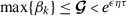
Given that (H1) and (H2) hold, the following conditions are fulfilled for \(k\in \mathbb{N}\):
-
(i)
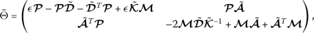
For given scalars \(\epsilon : 0<\epsilon < \min d_{i}\) (\(i=1,\ldots,n\)), \(\tau \geq 0\) and μ, if there exist positive definite matrices
 and
and  , and a positive diagonal matrix
  such that
 (13)
(13)where Θ is negative definite.
-
(ii)
For \(\gamma _{k}\geq 0\), \(k\in \mathbb{N}\), one can have
 .
. -
(iii)
For \(\eta >1\), one can have \(\eta \tau \leq \inf \{t_{k}-t_{k-1}\}\).
-
(iv)
 , \(k\in \mathbb{N}\), where
 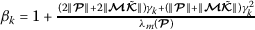 , where
  is a constant.
 and
and  , and a positive diagonal matrix
  such that

 .
. ,
,  , where
  is a constant.
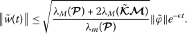
Then the equilibrium point of NN model (12) is globally exponentially stable. It has an exponential convergence rate ϵ. Moreover,

Proof
Construct a LKF for the NN model (12) as follows:

where \(\mathfrak{V}(t, \tilde{w}(t))\) is radially unbounded and  are positive definite matrices.
Based on Lemma (3.1), we have

When \(t\neq t_{k}\), \(k\in \mathbb{N}\), the time derivative of \(\mathfrak{V}(t, \tilde{w}(t))\) can be computed along the solutions of NN model (12), one obtains

From assumptions (H1) and (H2), one can get

From assumption (H2), one can obtain

Substituting (18) in (17), we have

where \(\zeta (t)=(\tilde{w}^{T}(t), \tilde{g}^{T}(\tilde{w}(t)), \tilde{g}^{T}( \tilde{w}(t-\tau (t))))^{T}\) and Θ is defined in (13).
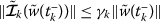
When \(t=t_{k}\), \(k\in \mathbb{N}\) by using (ii), (iii), we have

that is,
where  .
.
For any solution \(\tilde{w}(t, t_{0}, \tilde{w}_{0})\) of (3), by (19) and (20), we have

Since \(\eta \tau \leq \inf \{t_{k}-t_{k-1}\}\), one has \(k-1\leq \frac{(t_{k-1}-t_{0})}{\eta \tau }\), which implies

That is,

On the other hand

From (16), (23), (24), we have

that is,

By Definition 2.4, the NN model (12) is globally exponentially stable. The proof of Theorem 3.2 is completed. □
Remark 3.3
When the impulse effects are absent in the NN model (12),

By applying a similar approach to the one proposed in Theorem 3.2, the following global exponential stability criteria can be obtained for the NN model (26).
Corollary 3.4
Suppose (H1) and (H2) hold, then the following conditions are satisfied:
-
(i)
For given scalars \(\epsilon : 0<\epsilon < \min d_{i}\) (\(i=1,\ldots,n\)), \(\tau \geq 0\) and μ, if there exist positive definite matrices
 and
and  , and a positive diagonal matrix
  such that
 (27)
(27)where Θ̃ is negative definite.
 and
and  , and a positive diagonal matrix
  such that

As such, the equilibrium point of NN model (26) is globally exponentially stable. Further,

Proof
Construct the same LKF (15). The remaining proof follows the same procedure used for Theorem 3.2. Therefore, it is omitted here. □
Remark 3.5
With the absence of the time-varying delays and impulsive effects, NN model (12) reduces to the following model:

By applying a similar approach to the one proposed in Theorem 3.2, the following global exponential stability criteria can be obtained for NN model (29).
Corollary 3.6
Given (H1), the following conditions are satisfied:
-
(i)
For given scalars \(\epsilon : 0<\epsilon < \min d_{i}\) (\(i=1,\ldots,n\)), if there exist a positive definite matrix
 and a positive diagonal matrix
  such that
 (30)
(30)where Θ̄ is negative definite. As such, the equilibrium point pertaining to NN model (29) is globally exponentially stable. Moreover,
 (31)
(31)
 and a positive diagonal matrix
  such that


Proof
Construct the following LKF:

The remaining proof follows the one used for Theorem 3.2. Therefore, it is omitted here. □
Remark 3.7
The multiplication of Clifford numbers does not satisfy commutativity, which complicates the study of Clifford-valued NNs. As such, from the theoretical and practical point of view, studying the dynamical behaviors of Clifford-valued NNs are difficult tasks. On the other hand, the decomposition approach has proven to be very effective to overcome the difficulty of the non-commutativity of Clifford number multiplication. By decomposition approach, the original n-dimensional Clifford-valued system is decomposed into \(2^{m}n\)-dimensional real-valued system and the coefficient and activation functions of networks are explicitly expressed. Therefore, the decomposition approach is highly favorable to analyze the dynamics of Clifford-valued NNs. Most of authors have recently obtained sufficient criteria for Clifford-valued NN models using the decomposition method [34, 36, 38, 42].
Remark 3.8
In [35], fuzzy operations are incorporated into the Clifford-valued cellular NN model to investigate its \(S^{p}\)-almost periodic solutions. The effects of discrete delays in Clifford-valued recurrent NNs are considered in [36], and the associated globally asymptotic almost automorphic synchronization criteria are obtained. The leakage delay is introduced into Clifford-valued high-order Hopfield NN models in [39] to explore its existence and global exponential stability of almost automorphic solutions. To be compared with some previous studies of Clifford-valued NN models [33–42], in this paper, by considering a class of impulsive Clifford-valued NN system model, we have studied more realistic dynamical behavior. Therefore, the proposed results in this paper is different and new compared with those in the existing literature [33–42].
Remark 3.9
When we consider the exponential convergence rate \(\epsilon =0\) in the main results, the exponential stability criteria can be converted to asymptotically stability criteria.
4 Numerical Example
We present numerical simulation to ascertain the feasibility and effectiveness of the results established in Sect. 3.
Example 1
For \(m=2\) and \(n=2\), we have the following Clifford-valued impulsive NN model:

The number of the multiplication generators, \(e_{1}^{2}=e_{2}^{2}=e_{12}^{2}=e_{1}e_{2}e_{12}=-1\), \(e_{1}e_{2}=-e_{2}e_{1}=e_{12}\), \(e_{1}e_{12}=-e_{12}e_{1}=-e_{2}\), \(e_{2}e_{12}=-e_{12}e_{2}=e_{1}\), \(\dot{p}_{1}(t)=\dot{p}^{0}_{1}(t)e_{0}+\dot{p}^{1}_{1}(t)e_{1}+ \dot{p}^{2}_{1}(t)e_{2}+\dot{p}^{12}_{1}(t)e_{12}\), \(\dot{p}_{2}(t)=\dot{p}^{0}_{2}(t)e_{0}+\dot{p}^{1}_{2}(t)e_{1}+ \dot{p}^{2}_{2}(t)e_{2}+\dot{p}^{12}_{2}(t)e_{12}\). Furthermore, we take

According to their definitions, we have

and

It can be checked that when \(\epsilon =0.324\), \(\tau =0.8\), \(\mu =0.5\), \(\eta =2\) and \(\varsigma _{k}=(-1)^{k} (\frac{(e^{0.324}+2.6)}{2} )^{ \frac{1}{2}}\), \(k\in \mathbb{N}\), by using MATLAB, the LMI condition of (13) in Theorem 3.2 is true with \(t_{\min }=-0.0022\). The feasible solutions of the existing positive definite matrices  ,
,  and positive diagonal matrix
  are
are

As we know,

that is, \(\gamma _{k}=|\varsigma _{k}|-1\). Therefore,

Hence, when  , we have,
  , \(k\in \mathbb{N}\).
On the other hand, it is straightforward to ascertain that all conditions of Theorem 3.2 are fulfilled. Therefore, the unique equilibrium of NN model (12) is globally exponentially stable, which is verified by the numerical simulation. Under the initial condition \(\varphi _{1}(t)=-0.5e_{0}+0.9e_{1}-0.3e_{2}-0.7e_{12}\) for \(t\in [-\tau , 0]\), and \(\varphi _{2}(t)=0.6e_{0}-0.4e_{1}+0.2e_{2}+0.8e_{12}\) for \(t\in [-\tau , 0]\), the time responses of the state of NN model (33) \(p_{1}^{0}(t)\), \(p_{2}^{0}(t)\), \(p_{1}^{1}(t)\), \(p_{2}^{1}(t)\), \(p_{1}^{2}(t)\), \(p_{2}^{2}(t)\), \(p_{1}^{12}(t)\), \(p_{2}^{12}(t)\) with impulsive effects are presented in Figs. 1–5, respectively. When the impulse effects are absent in the NN model (33), the time responses of the states of NN model (33) \(p_{1}^{0}(t)\), \(p_{2}^{0}(t)\), \(p_{1}^{1}(t)\), \(p_{2}^{1}(t)\), \(p_{1}^{2}(t)\), \(p_{2}^{2}(t)\), \(p_{1}^{12}(t)\) are given in Figs. 6–10, respectively. It is obvious from Figs. 1–10 that the model converges to an equilibrium point, which means that model (33) is globally exponentially stable.

The time responses of the states \(p^{0}_{1}(t)\), \(p^{0}_{2}(t)\) of the NN model (33) with impulsive effects

The time responses of the states \(p^{1}_{1}(t)\), \(p^{1}_{2}(t)\) of NN model (33) with impulsive effects

The time responses of the states \(p^{2}_{1}(t)\), \(p^{2}_{2}(t)\) of NN model (33) with impulsive effects

The time responses of the states \(p^{12}_{1}(t)\), \(p^{12}_{2}(t)\) of NN model (33) with impulsive effects

The time responses of the states \(p_{1}^{0}(t)\), \(p_{2}^{0}(t)\), \(p_{1}^{1}(t)\), \(p_{2}^{1}(t)\), \(p_{1}^{2}(t)\), \(p_{2}^{2}(t)\), \(p_{1}^{12}(t)\), \(p_{2}^{12}(t)\) in a 2-dimensional space with impulsive effects

The time responses of the states \(p^{0}_{1}(t)\), \(p^{0}_{2}(t)\) of NN model (33) without impulsive effects

The time responses of the states \(p^{1}_{1}(t)\), \(p^{1}_{2}(t)\) of NN model (33) without impulsive effects

The time responses of the states \(p^{2}_{1}(t)\), \(p^{2}_{2}(t)\) of NN model (33) without impulsive effects

The time responses of the states \(p^{12}_{1}(t)\), \(p^{12}_{2}(t)\) of NN model (33) without impulsive effects

The time responses of the states \(p_{1}^{0}(t)\), \(p_{2}^{0}(t)\), \(p_{1}^{1}(t)\), \(p_{2}^{1}(t)\), \(p_{1}^{2}(t)\), \(p_{2}^{2}(t)\), \(p_{1}^{12}(t)\), \(p_{2}^{12}(t)\) in a 2-dimensional space without impulsive effects
5 Conclusion
In this study, the global exponential stability analysis pertaining to the Clifford-valued NN models with time-varying delays and impulsive effects has been comprehensively investigated. To tackle the problem, we firstly decomposed the considered n-dimensional Clifford-valued NN model into \(2^{m}n\)-dimensional real-valued ones. By using an appropriate Lyapunov functional and some inequality techniques, we have established new LMI-based sufficient conditions. These conditions guarantee the global exponential stability of the equilibrium point pertaining to the considered Clifford-valued NN model. To ascertain the validity of the main results, a standard numerical example has been provided. It is worth mentioning that the results achieved in this paper can further be extended to various complex systems. We will shortly attempt to explore the stabilization analysis of Clifford-valued NNs with the help of different controller schemes. The corresponding results will be presented in the near future.
Availability of data and materials
Data sharing is not applicable to this article as no datasets were generated or analysed during the current study.
References
Hopfield, J.J.: Neurons with graded response have collective computational properties like those of two-state neurons. Proc. Natl. Acad. Sci. USA 81, 3088–3092 (1984)
Hopfield, J.J., Tank, D.W.: Neural computation of decisions in optimization problems. Biol. Cybern. 52, 141–152 (1985)
Marcus, C.M., Westervelt, R.M.: Stability of analog neural networks with delay. Phys. Rev. A 39, 347–359 (1989)
Yang, R., Wu, B., Liu, Y.: A Halanay-type inequality approach to the stability analysis of discrete-time neural networks with delays. Appl. Math. Comput. 265, 696–707 (2015)
Cao, J., Ho, D.W.C.: A general framework for global asymptotic stability analysis of delayed neural networks based on LMI approach. Chaos Solitons Fractals 24, 1317–1329 (2005)
Kang, H., Zhou, H., Li, B.: Exponential stability of solution for delayed cellular neural networks with impulses. Proc. Eng. 15, 1626–1631 (2011)
Sakthivel, R., Sakthivel, R., Kaviarasan, B., Wang, C., Ma, Y.K.: Finite-time nonfragile synchronization of stochastic complex dynamical networks with semi-markov switching outer coupling. Complexity 2018, Article ID 8546304 (2018)
Kaviarasan, B., Kwon, O.M., Park, M.J., Sakthivel, R.: Composite synchronization control for delayed coupling complex dynamical networks via a disturbance observer-based method. Nonlinear Dyn. 99, 1601–1619 (2020)
Hirose, A.: Complex-valued neural networks: theories and applications. World Scientific, Singapore (2003)
Nitta, T.: Solving the XOR problem and the detection of symmetry using a single complex-valued neuron. Neural Netw. 16, 1101–1105 (2003)
Aouiti, C., Bessifi, M., Li, X.: Finite-time and fixed-time synchronization of complex-valued recurrent neural networks with discontinuous activations and time-varying delays. Circuits Syst. Signal Process. 39, 5406–5428 (2020)
Zhang, Z., Liu, X., Zhou, D., Lin, C., Chen, J., Wang, H.: Finite-time stabilizability and instabilizability for complex-valued memristive neural networks with time delays. IEEE Trans. Syst. Man Cybern. Syst. 48, 2371–2382 (2018)
Samidurai, R., Sriraman, R., Zhu, S.: Leakage delay-dependent stability analysis for complex-valued neural networks with discrete and distributed time-varying delays. Neurocomputing 338, 262–273 (2019)
Rajchakit, G., Sriraman, R.: Robust passivity and stability analysis of uncertain complex-valued impulsive neural networks with time-varying delays. Neural Process. Lett. 53, 581–606 (2021)
Isokawa, T., Nishimura, H., Kamiura, N., Matsui, N.: Associative memory in quaternionic Hopfield neural network. Int. J. Neural Syst. 18, 135–145 (2008)
Matsui, N., Isokawa, T., Kusamichi, H., Peper, F., Nishimura, H.: Quaternion neural network with geometrical operators. J. Intell. Fuzzy Syst. 15, 149–164 (2004)
Mandic, D.P., Jahanchahi, C., Took, C.C.: A quaternion gradient operator and its applications. IEEE Signal Process. Lett. 18, 47–50 (2011)
Li, Y., Meng, X.: Almost automorphic solutions for quaternion-valued Hopfield neural networks with mixed time-varying delays and leakage delays. J. Syst. Sci. Complex. 33, 100–121 (2020)
Tu, Z., Zhao, Y., Ding, N., Feng, Y., Zhang, W.: Stability analysis of quaternion-valued neural networks with both discrete and distributed delays. Appl. Math. Comput. 343, 342–353 (2019)
Shu, H., Song, Q., Liu, Y., Zhao, Z., Alsaadi, F.E.: Global μ-stability of quaternion-valued neural networks with non-differentiable time-varying delays. Neurocomputing 247, 202–212 (2017)
Liu, Y., Zhang, D., Lou, J., Lu, J., Cao, J.: Stability analysis of quaternion-valued neural networks: decomposition and direct approaches. IEEE Trans. Neural Netw. Learn. Syst. 29, 4201–4211 (2018)
Qi, X., Bao, H., Cao, J.: Exponential input-to-state stability of quaternion-valued neural networks with time delay. Appl. Math. Comput. 358, 382–393 (2019)
Jiang, B., Liu, Y., Kou, K.I., Wang, Z.: Controllability and observability of linear quaternion-valued systems. Acta Math. Sin. Engl. Ser. 36, 1299–1314 (2020)
Liu, Y., Zheng, Y., Lu, J., Cao, J., Rutkowski, L.: Constrained quaternion-variable convex optimization: A quaternion-valued recurrent neural network approach. IEEE Trans. Neural Netw. Learn. Syst. 31, 1022–1035 (2020)
Xia, Z., Liu, Y., Lu, J., Cao, J., Rutkowski, L.: Penalty method for constrained distributed quaternion-variable optimization. IEEE Trans. Cybern. (2020). https://doi.org/10.1109/TCYB.2020.3031687
Wang, H., Wei, G., Wen, S., Huang, T.: Impulsive disturbance on stability analysis of delayed quaternion-valued neural networks. Appl. Math. Comput. 390, 125680 (2021)
Pearson, J.K., Bisset, D.L.: Neural networks in the Clifford domain. In: Proc. IEEE ICNN, Orlando, FL, USA (1994)
Pearson, J.K., Bisset, D.L.: Back Propagation in a Clifford Algebra. In: ICANN (1992)
Pearson, J.K., Bisset, D.L.: An intorduction to Clifford Networks (1993)
Kuroe, Y.: Models of Clifford recurrent neural networks and their dynamics. In: IJCNN-2011, San Jose, CA, USA (2011)
Hitzer, E., Nitta, T., Kuroe, Y.: Applications of Clifford’s geometric algebra. Adv. Appl. Clifford Algebras 23, 377–404 (2013)
Buchholz, S.: A Theory of Neural Computation with Clifford Algebras. Ph.D. thesis, University of Kiel (2005)
Zhu, J., Sun, J.: Global exponential stability of Clifford-valued recurrent neural networks. Neurocomputing 173, 685–689 (2016)
Liu, Y., Xu, P., Lu, J., Liang, J.: Global stability of Clifford-valued recurrent neural networks with time delays. Nonlinear Dyn. 332, 259–269 (2019)
Shen, S., Li, Y.: \(S^{p}\)-Almost periodic solutions of Clifford-valued fuzzy cellular neural networks with time-varying delays. Neural Process. Lett. 51, 1749–1769 (2020)
Li, Y., Xiang, J., Li, B.: Globally asymptotic almost automorphic synchronization of Clifford-valued recurrent neural netwirks with delays. IEEE Access 7, 54946–54957 (2019)
Li, B., Li, Y.: Existence and global exponential stability of pseudo almost periodic solution for Clifford-valued neutral high-order Hopfield neural networks with leakage delays. IEEE Access 7, 150213–150225 (2019)
Li, Y., Xiang, J.: Global asymptotic almost periodic synchronization of Clifford-valued CNNs with discrete delays. Complexity 2019, Article ID 6982109 (2019)
Li, B., Li, Y.: Existence and global exponential stability of almost automorphic solution for Clifford-valued high-order Hopfield neural networks with leakage delays. Complexity 2019, Article ID 6751806 (2019)
Aouiti, C., Dridi, F.: Weighted pseudo almost automorphic solutions for neutral type fuzzy cellular neural networks with mixed delays and D operator in Clifford algebra. Int. J. Syst. Sci. 51, 1759–1781 (2020)
Aouiti, C., Gharbia, I.B.: Dynamics behavior for second-order neutral Clifford differential equations: inertial neural networks with mixed delays. Comput. Appl. Math. 39, 120 (2020)
Li, Y., Xiang, J.: Existence and global exponential stability of anti-periodic solution for Clifford-valued inertial Cohen–Grossberg neural networks with delays. Neurocomputing 332, 259–269 (2019)
Huang, T., Li, C., Duan, S., Starzyk, J.: Robust exponential stability of uncertain delayed neural networks with stochastic perturbation and impulse effects. IEEE Trans. Neural Netw. Learn. Syst. 23, 866–875 (2012)
Guan, Z.H., Chen, G.R.: On delayed impulsive Hopfield neural networks. Neural Netw. 12, 273–280 (1999)
Lakshmikantham, V., Bainov, D.D., Simeonov, P.S.: Theory of Impulsive Differential Equations. Ser. Modern Appl. Math., vol. 6. World Scientific, Teaneck (1989)
Long, S., Xu, D.: Delay-dependent stability analysis for impulsive neural networks with time varying delays. Neurocomputing 71, 1705–1713 (2008)
Gopalsamy, K.: Stability of artificial neural networks with impulses. Appl. Math. Comput. 154, 783–813 (2004)
Li, X., Wu, J.: Stability of nonlinear differential systems with state-dependent delayed impulses. Automatica 64, 63–69 (2016)
Rakkiyappan, R., Balasubramaniam, P., Cao, J.: Global exponential stability results for neutral-type impulsive neural networks. Nonlinear Anal., Real World Appl. 11, 122–130 (2010)
Li, Y., Xing, Z.: Existence and global exponential stability of periodic solution of CNNs with impulses. Chaos Solitons Fractals 33, 1686–1693 (2007)
Acknowledgements
This research is made possible through financial support from the Rajamangala University of Technology Suvarnabhumi, Thailand. The authors are grateful to the Rajamangala University of Technology Suvarnabhumi, Thailand for supporting this research.
Funding
The research is supported by the Rajamangala University of Technology Suvarnabhumi, Thailand.
Author information
Authors and Affiliations
Contributions
Funding acquisition, NB; Conceptualization, GR; Software, GR; Formal analysis, GR and NB; Methodology, GR and NB; Supervision, GR, PA, RS, PH and CPL; Writing–original draft, GR; Validation, GR and NB; Writing–review and editing, GR and NB. All authors have read and agreed to the published version of the manuscript.
Corresponding author
Ethics declarations
Competing interests
The authors declare that they have no competing interests.
Rights and permissions
Open Access This article is licensed under a Creative Commons Attribution 4.0 International License, which permits use, sharing, adaptation, distribution and reproduction in any medium or format, as long as you give appropriate credit to the original author(s) and the source, provide a link to the Creative Commons licence, and indicate if changes were made. The images or other third party material in this article are included in the article’s Creative Commons licence, unless indicated otherwise in a credit line to the material. If material is not included in the article’s Creative Commons licence and your intended use is not permitted by statutory regulation or exceeds the permitted use, you will need to obtain permission directly from the copyright holder. To view a copy of this licence, visit http://creativecommons.org/licenses/by/4.0/.
About this article

Cite this article
Rajchakit, G., Sriraman, R., Boonsatit, N. et al. Global exponential stability of Clifford-valued neural networks with time-varying delays and impulsive effects. Adv Differ Equ 2021, 208 (2021). https://doi.org/10.1186/s13662-021-03367-z
Received:
Accepted:
Published:
DOI: https://doi.org/10.1186/s13662-021-03367-z