
Abstract
This research proposes and delves into a stochastic competitive phytoplankton model with allelopathy and regime-switching. Sufficient criteria are proffered to ensure that the model possesses a unique ergodic stationary distribution (UESD). Furthermore, it is testified that these criteria are sharp on certain conditions. Some critical functions of regime-switching on the existence of a UESD of the model are disclosed: regime-switching could lead to the appearance of the UESD. The theoretical findings are also applied to research the evolution of Heterocapsa triquetra and Chrysocromulina polylepis.
1 Introduction
A global proliferation of harmful algal blooms (HABs) has caused significant harm to human and animal health, fisheries, tourism, ecosystem and environment in last decades [1]. For instance, according to the United States National Oceanic and Atmospheric Administration, HABs are responsible for more than 50% of improper decrease of marine mammals [2]; in addition, the United States Environmental Protection Agency estimated that HABs influence 65% of the major estuaries of the United States, costing $2.2 billion every year [3].
The toxins released by harmful phytoplankton may be responsible for HABs [4, 5]: the rise in density of a phytoplankton population may influence the growth of some other populations by producing allelopathic toxins or stimulator, leading to blooms [6]. Accordingly, in recent years, numerous phytoplankton models with allelopathy were dissected (see, e.g., [6–9]). Particularly, Bandyopadhyay [9] tested the following competitive model with allelopathy:
where \(\Psi _{i}\) means the population density, \(r_{i}>0\) represents the growth rate, \(\alpha _{ii}>0\) is the intraspecific competition rate, \(\alpha _{ij}>0\) (\(j\neq i\)) means the interspecific competition rate, \(i,j=1,2\); \(\beta >0\) measures the allelopathic interaction. In model (1), \(\beta \Psi _{1}^{2}\Psi _{2}^{2}\) is the allelopathic interaction term proposed by Solé et al. [8] based upon experimental data of two phytoplankton species, Heterocapsa triquetra and Chrysocromulina polylepis (the allelopathic species).
Nevertheless, the environmental random disturbances (for example, the variations of PH, temperature, and nutrition [10]) frequently act on the evolution of plankton [11–19]. Mandal and Banerjee [12] assumed that the environmental random disturbances are the white noise which mainly acts on the growth rates of the plankton with
they [12] tested the following stochastic competitive model with allelopathy:
where \(\gamma _{i}^{2}\) means the intensity of the white noise, \((B_{1}(t),B_{2}(t))\) is a two-dimensional Brownian motion defined on a certain complete probability space \((\Omega ,\mathcal{F},\{\mathcal{F}_{t}\}_{t\geq 0},\mathrm{P})\). The authors [12] tested the existence, uniqueness, boundedness, and stochastic permanence of the solution of model (2).
However, the growth rates of plankton organisms often shift from one regime to a dramatically different one because of some abrupt environmental disturbances (see [14, 18, 19]) which cannot be portrayed by the white noise. For example, the growth rate of microalgae at 30°C is about twice that at 20°C (see [10]). An effective approach to depict these abrupt disturbances is to make use of a continuous-time finite-state Markov chain (see [14, 18–21]). Let \(\eta =\eta (t)\) be an irreducible right-continuous Markov chain with the state space \(\mathbb{X}=\{1,\ldots,L\}\), the generator \((q_{ij})_{L\times L}\), and the stationary distribution π. Incorporating \(\eta (t)\) into system (2), we derive the following regime-switching model:
Stationary distribution (which can be regarded as a stable “stochastic positive equilibrium”) has propelled to the forefront in researches of stochastic models (see [13, 14, 19]). However, little research has been conducted to test the stationary distribution of model (2) or (3). For these reasons, in this paper, by taking advantage of some previous approaches and results mainly in [22], sufficient criteria are offered to ensure that model (3) possesses a unique ergodic stationary distribution (UESD) in Sect. 2. Furthermore, we proffer that the above criteria are sharp under certain conditions. In Sect. 3, some critical functions of regime-switching on the existence of a UESD of the model are disclosed and numerically manifested by means of some real data. Section 4 proffers the conclusions and the Appendix provides the mathematical proofs.
2 Theoretical results
For \(i=1,2\), consider the stochastic logistic equation below:
For Eq. (4), taking advantage of Theorem 6 in [23] results in
Furthermore, in accordance with [24], if \(\overline{a}_{i}>0\), then Eq. (4) possesses a UESD \(\Gamma _{i}(\cdot \times \cdot )\) on \(\mathbb{R}_{+}\times \mathbb{X}\), where
For model (3), it is trivial to check that if \(\overline{a}_{i}<0\), then the species i will become extinct, i.e., \(\lim_{t\rightarrow +\infty }\Psi _{i}(t)=0\), \(i=1,2\). Accordingly, from here on, we suppose that model (3) complies with \(\overline{a}_{1}>0\) and \(\overline{a}_{2}>0\).
Now we provide our first theoretical result.
Theorem 1
If \(\bar{b}_{1}>0\) and \(\bar{b}_{2}>0\), then model (3) possesses a UESD concentrated on \(\mathbb{R}_{+}^{2}\times \mathbb{X}\), where
Remark 1
If \(\alpha _{il}(\eta (t))\equiv \alpha _{il}\), a positive constant, \(i,l=1,2\), then model (3) is replaced by the following special case:
In light of [24], for model (4), if \(\overline{a}_{1}>0\) and \(\overline{a}_{2}>0\), one derives
Accordingly, for model (6),
An interesting problem follows from Theorem 1: what happens if \(\bar{b}_{1}<0\) or \(\bar{b}_{2}<0\)? For model (3), this problem is difficult, hence we test model (6) and derive the following results.
Theorem 2
For model (6), let \(\alpha _{11}\alpha _{22}>\alpha _{12}\alpha _{21}\).
-
(i)
If \(\overline{b}_{1}<0\), \(\overline{b}_{2}>0\), then species 1 becomes extinct and the transition probability of \((\Psi _{2}(t),\eta (t))\) converges weakly to \(\Gamma _{2}\).
-
(ii)
If \(\overline{b}_{1}>0\), \(\overline{b}_{2}<0\), then species 2 becomes extinct and the transition probability of \((\Psi _{1}(t),\eta (t))\) converges weakly to \(\Gamma _{1}\).
Remark 2
Under the assumption \(\alpha _{11}\alpha _{22}>\alpha _{12}\alpha _{21}\), one can deduce that \(\overline{b}_{1}<0\) and \(\overline{b}_{2}<0\) cannot be valid at the same time. Accordingly, under \(\alpha _{11}\alpha _{22}>\alpha _{12}\alpha _{21}\), sharp criteria for the existence of a UESD of model (6) are \(\overline{b}_{1}>0\) and \(\overline{b}_{2}>0\).
3 Discussions and applications
The theoretical results disclose several critical functions of regime-switching on the stability of system (3). To manifest these functions more directly, we probe model (6) with \(L=2\). Accordingly, system (6) jumps between the following two subsystems:
and
For models (8) and (9), suppose
We can deduce from Theorems 1 and 2 that
- (A):
-
if \(\overline{b}_{1}>0\) and \(\overline{b}_{2}>0\), then model (6) possesses a UESD concentrated on \(\mathbb{R}_{+}^{2}\times \mathbb{X}\);
- (B):
-
If \(\overline{b}_{1}<0\) and \(\overline{b}_{2}>0\), then species 1 becomes extinct and the transition probability of \((\Psi _{2}(t),\eta (t))\) converges weakly to \(\Gamma _{2}\);
- (C):
-
If \(\overline{b}_{1}>0\) and \(\overline{b}_{2}<0\), then species 2 becomes extinct and the transition probability of \((\Psi _{1}(t),\eta (t))\) converges weakly to \(\Gamma _{1}\).
Accordingly,
-
(I)
if both subsystems (8) and (9) possess the corresponding UESD on \(\mathbb{R}_{+}^{2}\) (i.e., \(b_{i}(j) > 0\), \(i, j = 1, 2\)), the hybrid model (6) still possesses a UESD on \(\mathbb{R}_{+}^{2}\times \{1,2\}\) owing to \(\overline{b}_{i}=\sum_{j=1,2}\pi _{j} b_{i}(j) >0\), \(i=1,2\).
-
(II)
An interesting question is what happens if one subsystem possesses a UESD on \(\mathbb{R}_{+}^{2}\) but the other does not. Under such circumstances, the hybrid model (6) may possess a UESD on \(\mathbb{R}_{+}^{2}\times \{1,2\}\) or not. If the Markov chain satisfies \(\overline{b}_{1}>0\) and \(\overline{b}_{2}>0\), then (6) possesses a UESD on \(\mathbb{R}_{+}^{2}\times \{1,2\}\); if the Markov chain satisfies \(\overline{b}_{1}<0\) or \(\overline{b}_{2}<0\), then a species in (6) will become extinct, namely, model (6) does not possess a stationary distribution on \(\mathbb{R}_{+}^{2}\times \{1,2\}\).
-
(III)
The case when neither (8) nor (9) possesses a stationary distribution on \(\mathbb{R}_{+}^{2}\) is similar to the case (II). Nevertheless, there is an interesting finding: under such circumstances, the hybrid system (6) could possess a UESD on \(\mathbb{R}_{+}^{2}\times \{1,2\}\), namely, the regime-switching could make the UESD on \(\mathbb{R}_{+}^{2}\times \{1,2\}\) appear.
Now let us reflect these functions by means of some real data of Heterocapsa triquetra and Chrysocromulina polylepis (the allelopathic species) presented by [8] (see Table 1).
Compute that
In accordance with (B) and (C), in state 1, Heterocapsa triquetra becomes extinct (see Fig. 1(a)) while in state 2, Chrysocromulina polylepis becomes extinct (see Fig. 1(b)). This suggests that neither subsystem (8) nor subsystem (9) possesses a stationary distribution on \(\mathbb{R}_{+}^{2}\). Now we let π change.
-
(I)
Let \(\pi =(0.5,0.5)\), then \(\overline{b}_{1}=\sum_{j=1,2}\pi _{j}b_{1}(j)=0.1491>0\), \(\overline{b}_{2}=0.2252>0\). In accordance with (A), the hybrid model (6) possesses a UESD on \(\mathbb{R}_{+}^{2}\times \{1,2\}\), see Fig. 1(c) and Fig. 1(d).
Figure 1 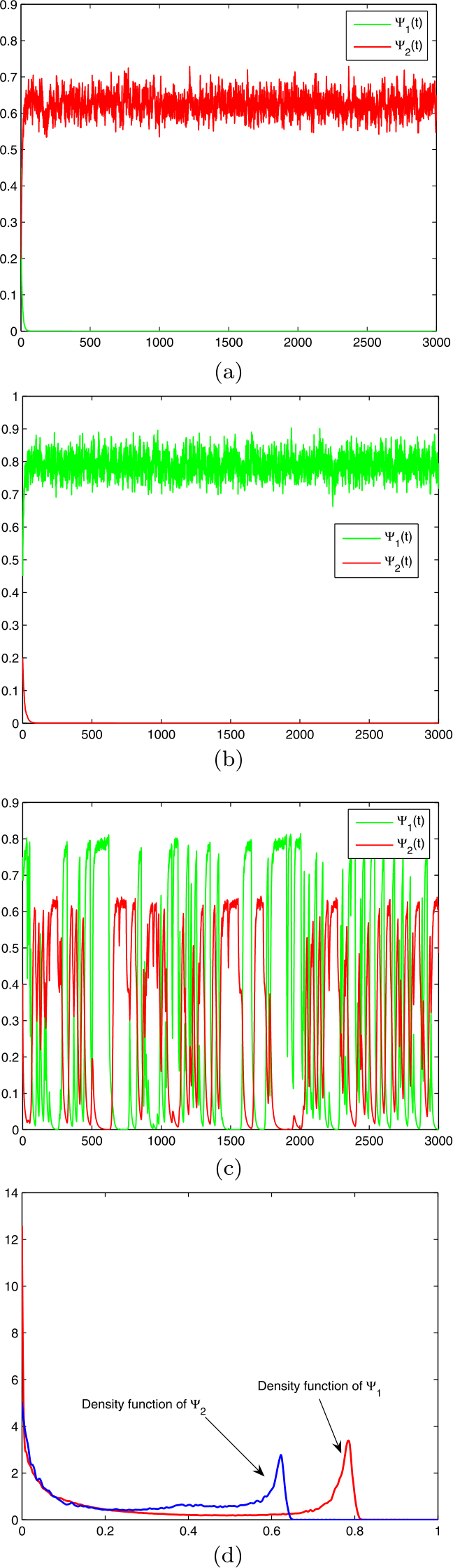
Model (6) with \(L=2\) and parameter values given in Table 1: (a) a trajectory of subsystem (8), which manifests that Heterocapsa triquetra becomes extinct; (b) a trajectory of subsystem (9), which manifests that Chrysocromulina polylepis becomes extinct; (c) a trajectory of the hybrid system (6), which manifests the two species are coexistent; and (d) the density function of the solution of the hybrid system (6) at \(t=3000\)
-
(II)
Let \(\pi =(0.96,0.04)\), then \(\overline{b}_{1}=-0.0029<0\), \(\overline{b}_{2}=0.445>0\). In accordance with (B), the first species, Heterocapsa triquetra, becomes extinct.
-
(III)
Let \(\pi =(0.03,0.97)\), then \(\overline{b}_{1}=0.305>0\), \(\overline{b}_{2}=-0.0015<0\). In accordance with (C), the allelopathic species, Chrysocromulina polylepis, becomes extinct.

4 Concluding remarks
In this article we developed a stochastic phytoplankton model with allelopathy and regime-switching, and offered sufficient criteria to ensure that the model possesses a UESD concentrated on \(\mathbb{R}_{+}^{2}\times \mathbb{X}\) (see Theorem 1). Furthermore, we proffered that the above criteria are sharp under certain conditions (see Remark 2). The results manifested that regime-switching could lead to the appearance of the UESD concentrated on \(\mathbb{R}_{+}^{2}\times \mathbb{X}\) (see Fig. 1).
Biologically, the existence of a UESD concentrated on \(\mathbb{R}_{+}^{2}\times \mathbb{X}\) suggests that the two species in model (3) are stably coexistent. As a result, the findings of this article suggest that if the Markov chain spends enough time in the desired state such that \(\bar{b}_{1}>0\) and \(\bar{b}_{2}>0\), then the two species in model (3) are stably coexistent; otherwise, the coexistence of the two species may be threatened, especially, if the Markov chain spends much more time in the undesired state such that \(\bar{b}_{i}<0\), then the species i in model (6) becomes extinct, \(i=1,2\).
Some issues deserve further investigation. To begin with, as pointed out above, for model (3), what happens if \(\overline{b}_{1}<0\) or \(\overline{b}_{2}<0\) is still unknown. Another interesting issue is to test other random perturbations, for instance, Lévy jumps. The motivation is that the evolution of plankton is frequently influenced by some abrupt disturbances which could not be depicted by model (3) and one might resort to the Lévy jumps. When the Lévy jumps are evaluated, model (3) is replaced by
where \(\mathcal{Z}\) is a subset of \(\mathbb{R}_{+}\), F̃ is a compensated Poisson random measure. Finally, for certain single-species model without switching, one can obtain the explicit form of the density function of the UESD (see, e.g., [25, 26]), the properties of the density function of the UESD of model (3) are unclear, yet. We leave the above three issues for further consideration.
Availability of data and materials
All data generated or analyzed during this study are included in this published article.
References
https://oceanservice.noaa.gov/news/weeklynews/dec08/dolphin_habs.html
Rice, E.: Allelopathy, 2nd edn. Academic Press, London (1984)
Chattopadhayay, J., Sarkar, R., Mandal, S.: Toxin-producing plankton may act as a biological control for planktonic blooms-field study and mathematical modelling. J. Theor. Biol. 215, 333–344 (2002)
Maynard-Smith, J.: Models in Ecology. Cambridge University Press, Cambridge (1974)
Chattopadhyay, J.: Effects of toxic substances on a two-species competitive system. Ecol. Model. 84, 287–289 (1996)
Solé, J., García-Ladona, E., Ruardij, P., Estrada, M.: Modelling allelopathy among marine algae. Ecol. Model. 183, 373–384 (2005)
Bandyopadhyay, M.: Dynamical analysis of a allelopathic phytoplankton model. J. Biol. Syst. 14, 205–218 (2006)
Flynn, K., Raven, J.: What is the limit for photoautotrophic plankton growth rates? J. Plankton Res. 39, 13–22 (2017)
Bandyopadhyay, M., Saha, T., Pal, R.: Deterministic and stochastic analysis of a delayed allelopathic phytoplankton model within fluctuating environment. Nonlinear Anal. Hybrid Syst. 2, 958–970 (2008)
Mandal, P., Banerjee, M.: Deterministic and stochastic dynamics of a competitive phytoplankton model with allelopathy. Differ. Equ. Dyn. Syst. 21, 341–372 (2013)
Wu, R., Zou, X., Wang, K.: Dynamical behavior of a competitive system under the influence of random disturbance and toxic substances. Nonlinear Dyn. 77, 1209–1222 (2014)
Zhao, Y., Yuan, S., Zhang, T.: The stationary distribution and ergodicity of a stochastic phytoplankton allelopathy model under regime switching. Commun. Nonlinear Sci. Numer. Simul. 37, 131–142 (2016)
Yu, X., Yuan, S., Zhang, T.: The effects of toxin-producing phytoplankton and environmental fluctuations on the planktonic blooms. Nonlinear Dyn. 91, 1653–1668 (2018)
Yu, X., Yuan, S., Zhang, T.: Asymptotic properties of stochastic nutrient-plankton food chain models with nutrient recycling. Nonlinear Anal. Hybrid Syst. 34, 209–225 (2019)
Zhao, S., Yuan, S., Wang, H.: Threshold behavior in a stochastic algal growth model with stoichiometric constraints and seasonal variation. J. Differ. Equ. 268, 5113–5139 (2020)
Chen, Z., Tian, Z., Zhang, S., Wei, C.: The stationary distribution and ergodicity of a stochastic phytoplankton–zooplankton model with toxin-producing phytoplankton under regime switching. Physica A 537, 122728 (2020)
Wang, H., Liu, M.: Stationary distribution of a stochastic hybrid phytoplankton–zooplankton model with toxin-producing phytoplankton. Appl. Math. Lett. 101, 106077 (2020)
Liu, M., Bai, C.: Optimal harvesting of a stochastic mutualism model with regime-switching. Appl. Math. Comput. 375, 125040 (2020)
Li, D., Liu, M.: Invariant measure of a stochastic food-limited population model with regime switching. Math. Comput. Simul. 178, 16–26 (2020)
Hening, A., Nguyen, D.: Coexistence and extinction for stochastic Kolmogorov systems. Ann. Appl. Probab. 28, 1893–1942 (2018)
Liu, M., Wang, K.: Asymptotic properties and simulations of a stochastic logistic model under regime switching II. Math. Comput. Model. 55, 405–418 (2012)
Liu, M.: Dynamics of a stochastic regime-switching predator-prey model with modified Leslie–Gower Holling-type II schemes and prey harvesting. Nonlinear Dyn. 96, 417–442 (2019)
Ji, W., Zhang, Y., Liu, M.: Dynamical bifurcation and explicit stationary density of a stochastic population model with Allee effects. Appl. Math. Lett. 111, 106662 (2021)
Ji, W., Hu, G.: Stability and explicit stationary density of a stochastic single-species model. Appl. Math. Comput. 390, 125593 (2021)
Nguyen, D., Yin, G., Zhu, C.: Certain properties related to well posedness of switching diffusions. Stoch. Model. Appl. 127, 3135–3158 (2017)
Meyn, S., Tweedie, R.: Markov Chains and Stochastic Stability. Springer, London (1993)
Yin, G., Zhu, C.: Hybrid Switching Diffusions: Properties and Applications. Springer, New York (2010)
Ikeda, N., Watanabe, S.: Stochastic Differential Equations and Diffusion Processes. North-Holland, New York (1989)
Acknowledgements
Not applicable.
Funding
ZJW thanks the National Natural Science Foundation of China (No. 11771174) and Natural Science Foundation of Jiangsu Province, China (No. BK20170067).
Author information
Authors and Affiliations
Contributions
WJ mainly finished the writing of the whole content of the paper. ZW and GH mainly finished the establishment of model and development. All authors read and approved the final manuscript.
Corresponding author
Ethics declarations
Competing interests
The authors declare that they have no competing interests.
Appendix
Appendix
For simplicity, define
There are positive constants Ξ and \(\mu <1\) such that for \(\forall (\Psi ,j)\in \overline{\mathbb{R}}_{+}^{2}\times \mathbb{X}\) with \(\Vert \Psi \Vert \geq \Xi \),
where \(\overline{\mathbb{R}}_{+}^{2}=\{x_{1}\geq 0,x_{2}\geq 0\}\). Accordingly, for \(\forall \chi \in (0,\min \{\mu /2,\mu /(2\widehat{\gamma ^{2}}) \} )\) and \(\Vert \Psi \Vert \geq \Xi \),
where \(\widehat{\gamma ^{2}}=\max_{i=1,2} \{\max_{j\in \mathbb{X}}\{\gamma _{i}^{2}(j)\} \}\). This suggests that
For all \(\widetilde{\kappa }=(\widetilde{\kappa }_{1},\widetilde{\kappa }_{2}) \in \mathbb{R}_{+}^{2}\) such that \(\Vert \widetilde{\kappa } \Vert \leq \chi <1/2\), define
It follows that \(\forall (\Psi ,j)\in \mathbb{R}_{+}^{2}\times \mathbb{X}\), \(\widetilde{U}(\Psi ,j)>1\).
Consider the following equation:
for any \(j\in \mathbb{X}\) and arbitrary twice continuously differentiable function \(U(\cdot ,j)\), and define
where \((q_{ij})_{L\times L}\) means the generator of \(\eta (t)\).
Lemma 1
For any \((\Psi (0),\eta (0))=(\nu ,j)\in \mathbb{R}_{+}^{2}\times \mathbb{X}\), model (3) possesses a unique solution \((\Psi (t),\eta (t))\in \mathbb{R}_{+}^{2}\times \mathbb{X}\) for all \(t\geq 0\), which is a Markov–Feller process, and
Proof
The proof of the first claim is similar to that of [14] and therefore is left out. Now we consider the second claim. On the basis of (12), one obtains
Furthermore, one has
In accordance with (14), (15), and Theorem 5.1 in [27], \((\Psi (t),\eta (t))\) possesses the Markov–Feller property. Taking advantage of (14) and the Gronwall inequality yields the last declaration. □
When \(\overline{b}_{1}>0\) and \(\overline{b}_{2}>0\), choose a \(\kappa =(\kappa _{1},\kappa _{2})^{\mathrm{T}}\in \mathbb{R}_{+}^{2}\) fulfilling \(\Vert \kappa \Vert \leq \chi <1/2\). Define
Lemma 2
If \(\overline{b}_{1}>0\) and \(\overline{b}_{2}>0\), then there is a positive constant ρ such that for any \(t\geq \rho \) and \((\Psi (0),\eta (0))=(\widetilde{\nu },j)\in \partial \mathbb{R}_{+}^{2} \times \mathbb{X}\) fulfilling \(\Vert \widetilde{\nu } \Vert \leq \Xi \),
where \(\partial \mathbb{R}_{+}^{2}=\overline{\mathbb{R}}_{+}^{2}\setminus \mathbb{R}_{+}^{2}\),
Proof
(a) Suppose \(\Psi _{1}(0)=\Psi _{2}(0)=0\). It follows that \(\Psi _{1}(t)=\Psi _{2}(t)\equiv 0\), \(t\geq 0\), and
We can deduce from the ergodicity of η that
This yields (17).
(b) Suppose \(\Psi _{1}(0)=0\), \(\Psi _{2}(0)>0\). Thus \(\Psi _{1}(t)\equiv 0\), \(\Psi _{2}(t)=\widetilde{\Psi }_{2}(t)\), \(t\geq 0\), where \(( \widetilde{\Psi }_{2}(t),\eta (t))\) is the solution of model (4) with \(i=2\). We can see that
Notice that \(\overline{a}_{2}>0\), and hence Eq. (4) (\(i=2\)) possesses a UESD \(\Gamma _{2}(\cdot \times \cdot )\). In accordance with Itô’s formula, one can deduce from the strong law of large numbers and the ergodicity of \(\Gamma _{2}\) that
Since
inequality (5) implies that \(\lim_{t\rightarrow +\infty }t^{-1}\ln (1+ \widetilde{\Psi }_{2}(t))=0\). Accordingly,
One can deduce from (7), (18), and the ergodicity of \(\Gamma _{2}\) and (19) that
(c) Suppose \(\Psi _{1}(0)>0\), \(\Psi _{2}(0)=0\). The proof is analogous and hence left out. □
Lemma 3
If \(\overline{b}_{1}>0\) and \(\overline{b}_{2}>0\), then there are a couple of constants \(\Upsilon \in (0,\chi /2)\) and \(\theta _{\Upsilon }>0\) such that for any \(t\in [\rho ,M^{\ast }\rho ]\) and \((\Psi (0),\eta (0))=(\nu ,j)\in \mathbb{R}_{+}^{2}\times \mathbb{X}\) fulfilling \(\Vert \nu \Vert \leq \Xi \),
where \(M^{\ast }\in \mathbb{N}\) and
Proof
We can deduce from Itô’s formula that
Then (13) purports that
Define
Tanking advantage of Itô’s formula again results in
Because
inequality (23) suggests that
We then deduce from (22) that for \(t\in [\rho ,M^{\ast }\rho ]\),
Define
Then (24) and Lemma 3.5 in [22] purport that \(\Phi _{\nu ,j,t}(z)\) is twice differentiable for \(z\in [0,\chi /2)\), and there exists a constant \(\theta _{3}>0\) which depends only on \(\theta _{2}\) such that for any \(z\in [0,\chi /2)\), \(t\in [\rho ,M^{\ast }\rho ]\),
Because \((\Psi (t),\eta (t))\) is Feller and (17) is validated, we can find a \(\theta _{4}>0\) such that for \(0<\operatorname{dist} (\nu ,\partial \mathbb{R}^{2}_{+})<\theta _{4}\),
Expanding \(\Phi _{\nu ,j,t}(z)\) around 0, then taking advantage of (25) and (26), one can derive that there is a sufficiently small ϒ such that
Then (22) purports that for \(0<\operatorname{dist}(\nu ,\partial \mathbb{R}^{2}_{+})<\theta _{4}\) and \(t\in [\rho ,M^{\ast }\rho ]\),
If \(\operatorname{dist}(\nu ,\partial \mathbb{R}^{2}_{+})\geq \theta _{4}\), for \(\Vert \nu \Vert \leq \Xi \) and \(t\in [\rho ,M^{\ast }\rho ]\), (13) purports that
Therefore, (20) is validated. □
Proof of Theorem 1
Define
In accordance with (14), we have
Then (11) purports that
Taking advantage of Dynkin’s formula yields
For this reason,
Because \((\Psi (t),\eta (t))\) has the Markov property and (20) is validated, we obtain
In the same way, (13) purports that
We can deduce from (27), (28), and (29) that
where \(\theta _{5}>0\) is a constant. Accordingly,
Additionally, it is standard (see, e.g., [22]) to show that \(\{ (\Psi (jM^{\ast }\rho ),\eta (jM^{\ast }\rho ) ) \}_{j \in \mathbb{N}}\) is aperiodic and irreducible, and any compact set \(A\in \mathbb{R}^{2}_{+}\) is petite. Then Theorem 15.0.1 in [28] purports that \(\{ (\Psi (j M^{\ast }\rho ),\eta (j M^{\ast }\rho ) ) \}_{j \in \mathbb{N}}\) is positively recurrent. Accordingly, \(\{ (\Psi (t),\eta (t) ) \}\) is positively recurrent. Then [29] (Theorems 4.3 and 4.4) suggests that model (3) possesses a UESD on \(\mathbb{R}_{+}^{2}\times \mathbb{X}\). □
Proof of Theorem 2
We only prove (i), the proof of (ii) is analogous to that of (i) and hence left out.
On the basis of the comparison theorem for stochastic equations [30], one observes \(\Psi (t)\leq \widetilde{\Psi }(t)\) for \(t\geq 0\), \(i=1,2\). Then (5) purports that
Taking advantage of Itô’s formula in (6) results in
Computing \(\text{(32)}\times \alpha _{22}-\text{(33)}\times \alpha _{12}\), we have
Accordingly,
Taking the superior limit of both sides, and then applying (31) and the fact that
we have
For this reason, \(\lim_{t\rightarrow +\infty }\Psi _{1}(t)=0\). Accordingly, the transition probability of \((\Psi _{2}(t),\eta (t))\) converges weakly to \(\Gamma _{2}\). □
Rights and permissions
Open Access This article is licensed under a Creative Commons Attribution 4.0 International License, which permits use, sharing, adaptation, distribution and reproduction in any medium or format, as long as you give appropriate credit to the original author(s) and the source, provide a link to the Creative Commons licence, and indicate if changes were made. The images or other third party material in this article are included in the article’s Creative Commons licence, unless indicated otherwise in a credit line to the material. If material is not included in the article’s Creative Commons licence and your intended use is not permitted by statutory regulation or exceeds the permitted use, you will need to obtain permission directly from the copyright holder. To view a copy of this licence, visit http://creativecommons.org/licenses/by/4.0/.
About this article

Cite this article
Ji, W., Wang, Z. & Hu, G. Stationary distribution of a stochastic hybrid phytoplankton model with allelopathy. Adv Differ Equ 2020, 632 (2020). https://doi.org/10.1186/s13662-020-03088-9
Received:
Accepted:
Published:
DOI: https://doi.org/10.1186/s13662-020-03088-9