
Abstract
The prevalence of the use of mathematical software has dramatically influenced the evolution of differential equations. The use of these useful tools leads to faster advances in the presentation of numerical and analytical methods. This paper retrieves several soliton solutions to the fractional perturbed Schrödinger’s equation with Kerr and parabolic law nonlinearity, and local conformable derivative. The method used in this article, called the generalized exponential rational function method, also relies heavily on the use of symbolic software such as Maple. The considered model has prominent applications in water optical metamaterials. The method retrieves several exponential, hyperbolic, and trigonometric function solutions to the model. The numerical evolution of the obtained solutions is also exhibited. The resulted wide range of solutions derived from the method proves its effectiveness in solving the model under investigation. It is also recommended to use the technique used in this article to solve similar problems.
1 Introduction
In general, it is complicated to find an analytical solution to many partial differential equations. Nowadays, almost all methods of solving differential equations, either numerically or analytically, rely on the use of computer software. In some cases, analytical solutions to such equations may not be found. Along with the astonishing advances in computer science and the reinforcement of mathematical software, there have also been fundamental changes in analytical methods [1, 3, 4, 7, 10, 11, 18–20, 22, 25, 26, 28–30, 32, 33]. The essence of many of these methods is to perform complicated calculations that would not be possible without the use of computer equipment. In this paper, we study the perturbed nonlinear Schrödinger’s equation given by [5, 6, 8, 9, 31]:

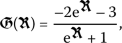
In this model, the complex-valued dependent variable is  , and
, and  is its complex conjugate; a is the group velocity dispersion, while \(b_{1}\) and \(b_{2}\) together comprise the quadratic–cubic nonlinearity. On the right-hand side, σ is the intermodal dispersion, while β and γ respectively represent the self-steepening and nonlinear dispersion. Finally, the terms with \(\theta _{i}\) for \(i = 1, 2, 3\) appear in the context of metamaterials. The readers who are interested in getting more information about the model and its applications can refer to the references [5, 6, 8, 9, 31]. Due to the very high importance of this equation, many researchers have been interested in finding analytical solutions to the equation, and several integration tools have been adopted to obtain its wave solutions. In [6], two integration methods, including the ansatz and the simplest equation approaches, have been applied to derive several singular 1-soliton solutions to Eq. (1). They have also introduced several topological soliton, rational, and singular periodic solutions obtained mainly from the simplest equation method. The mapping method has been utilized to achieve several soliton solutions to the model via Kerr and parabolic law nonlinearity in [31]. The authors in [8] have investigated the model and got a W-shaped soliton solution and a bright soliton solution to the model. They have also presented the numerical evolution of the obtained solutions. The main difference between the present work and those mentioned above is the use of a newly-defined derivative, called conformable derivative. Two efficient algorithms, including the \(\exp (-\phi (\eta ))\)-expansion method and extended Jacobi’s elliptic function expansion method have been utilized in [9] to examine the mathematical analysis of the considered equation (1). The result of this study was the determination of analytical dark soliton, singular soliton, and periodic solutions. Taking specific limit values, achieved elliptic solutions are turned into solitary, shock, and singular wave solitons. The elliptic waves acquired by the extended Jacobi’s elliptic function expansion technique are reduced to solitary waves, shock waves, and singular solitons in some specific limiting situations. Besides, several waves, such as plane waves as well as bright and singular solitons of periodic type, have been retrieved via the extended trial equation [9]. In [5], several 1-soliton solutions varieties of the bright and dark soliton solutions to the governing model were extracted through implementations of the ansatz integration technique.
The main difference between the present work and those mentioned above is the use of a new definition for the derivative in the equation, the so-called conformable derivative. This definition for the derivative was first proposed by Khalil et al. in [23] as a natural extension of the usual derivative. The generalized exponential rational function method has been utilized to solve extended Zakharov–Kuzetsov equation with conformable derivative in [17]. In [21], a generalized type of conformable local fractal derivative (GCFD) is employed to investigate some nonlinear evolution equations. The authors have also set up a general technique to find exact solutions for their studied PDEs. In [24], the modified Kudryashov method has been employed to construct the solutions to the conformable time fractional regularized long wave Burgers equation. In [2], several wave solutions for time-fractional nonlinear dispersive PDEs in the sense of conformable fractional derivative have been obtained. The definition has many of the important features of a standard derivative. This is the main advantage of this definition. This derivative has been widely used in research works in the literature. For example, in [2] a fuzzy approach to conformable fractional differential equations has been investigated, and modern trend and new computational algorithm in terms of analytic and approximate conformable solutions have been proposed. Very recently, in [12], the authors have studied some new optical wave solutions of the Gerdjikov–Ivanov equation involving conformable derivative. We also use the generalized exponential rational function method (GERFM) [14] to solve this fractional model. It is important to note that this method has not been elaborated for the considered form of equation in the previous literature. This article has the following general structure. In Sect. 2, we will present some mathematical background and methodologies. This chapter will include details of the GERFM, and general principles of the fractional conformable derivative. The perturbed nonlinear Schrödinger’s equation is defined in Sect. 3. In Sect. 4, several numerical simulations are given. Finally, conclusions are drawn in the last section.
2 Mathematical methodologies and background
This section first provides the main structure of the GERFM. Then the basic concepts of the conformable derivative will be expressed.
2.1 Description of GERFM
The authors in [14] have developed an integration technique called GERFM to solve the resonance nonlinear Schrödinger equation. Following their achievement, several successful works have been conducted in solving different PDEs [12, 13, 15–17, 27]. We will also apply this technique as the main method of the article. Now, let us briefly describe the main steps of the process:
-
1.
Consider a typical nonlinear PDE for
 , given by
 (2)
(2)Under the wave transformation of
 with
with  , Eq. (2) becomes an ordinary differential equation given by
 (3)
(3) -
2.
Now, we assume that Eq. (3) admits the exact solution given by
 (4)
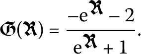
(4)where
 (5)
(5)and
 ,
,  ’s and \(\mathcal{A}_{0}\), \(\mathcal{A}_{k}\) and \(\mathcal{B}_{k}\)’s are appropriate parameters, and also
  is evaluated by applying the homogeneous balance to (3).
 -
3.
Inserting Eq. (4) into (3) with Eq. (5), and then gathering all possible powers of
 for \(k=1,\ldots ,4\), yields a polynomial equation
  . Equating the coefficients of P to zero, one derives a simultaneous system of equations in
  ,
,  , and σ, l, \(\mathcal{A}_{0}\), \(\mathcal{A}_{k}\) and
  .
. -
4.
Finally, solving the nonlinear system and substituting the obtained solutions into Eqs. (4) and (5), the explicit form of the solutions of (2) will be determined.
 , given by

 with
with  , Eq. (


 ,
,  ’s and
  is evaluated by applying the homogeneous balance to (
 for
for  . Equating the coefficients of P to zero, one derives a simultaneous system of equations in
  ,
,  , and σ, l,
  .
.2.2 Description of the conformable derivative
Definition
The conformable derivative of  of order \({\alpha }\in (0,1]\) at \(t=t_{0}\), is given by [23]

It is clear that for \(\alpha =1\), this definition will reduce to the standard definition for the derivative.
Theorem
For any\({\alpha }\in (0,1] \), and two conformable-differentiable functions ,
,  , we get
-
 .
. -
 , for\(c_{1} ,c_{2} \in \mathbb{R}\).
 -
 , for\(c \in \mathbb{R}\).
 -
 .
. -
 .
. -
If
 is a differentiable function (in the standard sense), then
 holds.
 .
. , for
, for , for
, for .
. .
. is a differentiable function (in the standard sense), then
 holds.
Since many of the existing definitions do not have some of these features, the existence of these features is one of the advantages of this definition.
Theorem
Let be a function such that it is classically and conformably differentiable. Moreover, suppose that
 is a differentiable function defined on the range of
 . Then we have

where primes stand for standard derivatives with respect tot.
3 The main results
The main purpose of this article is to apply the derivatives defined by (6) in the main equation (1) as follows:

To solve the main PDE, we first need to consider the following new complex transformations:

where  ,
,  ,
,  , and
, and  are unknown values which need to be determined.
Inserting Eq. (8) into Eq. (7), after doing some cumbersome manipulations, reduces the original PDE to two equations from the real and imaginary parts. The imaginary part yields

and

Also, from the real part we have

Then imposing the conditions \(\theta _{1}=0\) and \(\theta _{2}=-\theta _{3}\) in (10) and (11), we get respectively [9]:

and

Now, applying the balancing principle to Eq. (13) for  and
and  suggests
  , therefore
  .
.
Taking into account Eq. (5) along with  gives
gives

Substituting (14) into (13) and pursuing the steps outlined for the method, the exact closed-form solutions to the partial differential equation (7) will be determined.
- Set 1.:
-
If one considers
 and
and  , Eq. (5) will turn into
 (15)
(15)which yields
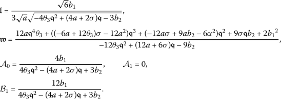
- Case I.:
-
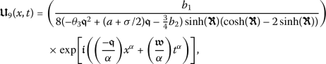
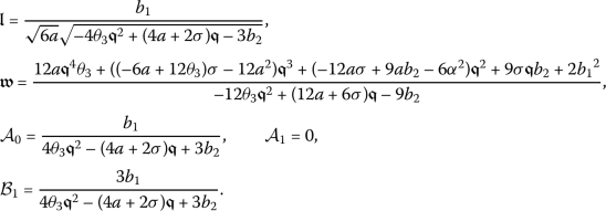
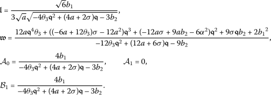
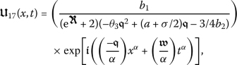
Taking into account these values, along with (14) and (15), gives

Accordingly, we will determine a wave solution for the conformable PDE (7) as
 (16)
(16)where
- Case II.:
-
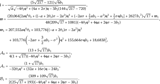
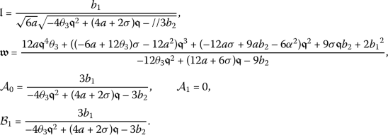
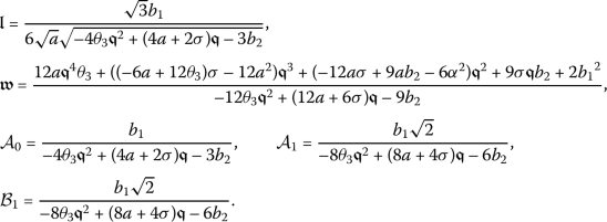
Taking into account these values, along with (14) and (15), yields

As a result, one derives a wave solution for the conformable PDE (7) as
 (17)
(17)where

- Case III.:
-
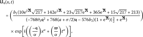
Taking into account these values, along with (14) and (15), one obtains

Hence, a new soliton solution for the conformable PDE (7) is constructed as
 (18)
(18)where

- Case IV.:
-

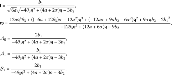
Taking into account these values, along with (14) and (15), one achieves

Consequently, a wave solution for the conformable PDE (7) is resulted as
 (19)
(19)where

- Set 2.:
-
If one considers
 and
and  , then Eq. (5) will turn into
 (20)
(20) - Case I.:
-
Taking into account these values, along with (14) and (20), yields the following result:

Thus, we will determine a wave solution for the conformable PDE (7) as

- Case II.:
-
Taking into account these values, along with (14) and (20), yields
Accordingly, we will determine a wave solution for the conformable PDE (7) as
 (21)
(21)where
- Set 3.:
-
If one considers
 and
and  , then Eq. (5) will turn into
 (22)
(22) - Case I.:
-
Taking into account these values, along with (14) and (22) yields

Consequently, we will determine a wave solution for the conformable PDE (7) as
 (23)
(23)where

- Case II.:
-

Taking into account these values, along with (14) and (22), one gets

Consequently, a novel soliton solution for the conformable PDE (7) is constructed as

where

- Set 4.:
-
If one considers
 and
and  , then Eq. (5) will turn into
 (24)
(24) - Case I.:
-
Taking into account these values, along with (14) and (24), yields

As a result, we will determine a wave solution for the conformable PDE (7) as
 (25)
(25)where

- Case II.:
-
Taking into account these values, along with (14) and (24), yields

Accordingly, one will obtain a novel solution for the conformable problem (7) as
 (26)
(26)where

- Case III.:
-
Taking into account these values, along with (14) and (24), yields

Consequently, we will determine a wave solution for the conformable equation (7) as
 (27)
(27)where

- Set 5.:
-
If one considers
 and
and  , then Eq. (5) will turn into
 (28)
(28) - Case I.:
-

Taking into account these values, along with (14) and (28), yields

As a result, we will determine a wave solution for the conformable formulation (7) as
 (29)
(29)where

- Case II.:
-

Taking into account these values, along with (14) and (28), yields
Accordingly, we will determine a wave solution for the conformable equation (7) as
 (30)
(30)where

- Case III.:
-

Taking into account these values, along with (14) and (28), yields
As a result, we will determine a wave solution for the conformable partial differential equation (7) as
 (31)
(31)where

- Set 6.:
-
If one considers
 and
and  , then Eq. (5) will turn into
 (32)
(32) - Case I.:
-

Taking into account these values, along with (14) and (32), yields
Consequently, we will determine a wave solution for the conformable partial differential equation (7) as
 (33)
(33)where

- Case II.:
-

Taking into account these values, along with (14) and (32), yields

Consequently, we will determine a wave solution for the conformable equation (7) as
 (34)
(34)where

- Set 7.:
-
If one considers
 and
and  , then Eq. (5) will turn into
 (35)
(35) - Case I.:
-
Taking into account these values, along with (14) and (35), yields

Accordingly, we will derive a wave solution for the conformable problem (7) as
 (36)
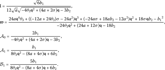
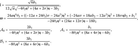
(36)where

- Case II.:
-

Taking into account these values, along with (14) and (35), yields

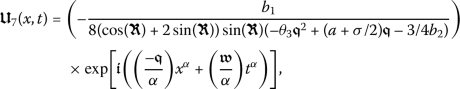
As a result, we will determine a novel wave solution for the conformable PDE (7) as
 (37)
(37)where

- Set 8.:
-
If one considers
 and
and  , then Eq. (5) will turn into
 (38)
(38) - Case I.:
-
Taking into account these values, along with (14) and (38), yields
Consequently, we will obtain a wave solution for the conformable equation (7) as
 (39)
(39)where

 and
and  , Eq. (


 and
and  , then Eq. (


 and
and  , then Eq. (


 and
and  , then Eq. (


 and
and  , then Eq. (


 and
and  , then Eq. (


 and
and  , then Eq. (


 and
and  , then Eq. (


To the best of our knowledge, all the acquired results obtained in this article are resented for the first time. In addition, in order to investigate the correctness of each of the solutions, we have substituted them into the main equation, and found that all solutions satisfied it.
4 Numerical simulations
In this section, we depict the obtained solutions for the perturbed nonlinear Schrödinger’s equation. Now, we will discuss the possible physical significance for the parameters. Figure 1 depicts the dynamic behavior of  when \(a = 0.1\), \(b_{1}= 0.5\), \(b_{2} = 1\), \(\beta = 1\), \(\gamma = 1\), \(\theta _{3} = 0.2\), and \(\sigma =-3.47\) are considered. In each row of this figure, the graphs are plotted for a specific value for the fractional order α.

Dynamic behavior of 
Figure 2 shows the dynamic behavior for  . In this figure we have used \(a = 2.5\), \(b_{1}= 0.01\), \(b_{2} = 0.05\), \(\beta =0.21\), \(\gamma =0.7\), \(\theta _{3} = 1.5\), and \(\sigma =-6.63\). It is clearly seen that by changing the fractional order α the behavior of the solutions will also be affected. In Fig. 3 we have also plotted
  for \(a = 0.01\), \(b_{1}= 0.01\), \(b_{2} = 0.5\), \(\beta =0.3\), \(\gamma =0.2\), \(\theta _{3} = 0.01\), and \(\sigma =-0.7\). Taking \(a = 0.005\), \(b_{1}= 0.1\), \(b_{2} = 0.5\), \(\beta =0.5\), \(\gamma =0.2\), \(\theta _{3} = 0.01\), and \(\sigma =-0.98\) in (7), the solution given by
  has been plotted in Fig. 4. When α changes, the range of solutions and the dynamic behavior of each also changes. The effects of the parameters are evident in the diagrams. In Fig. 5, we present the numerical simulations of
  for \(a = 0.005\), \(b_{1}= 0.01\), \(b_{2} = 0.5\), \(\beta =0.5\), \(\gamma =1.2\), \(\theta _{3} = 0.07\), and \(\sigma =-2.01\), when α is taken 0.5, 0.75, and 0.98. The same situation has been considered in Fig. 6 where
  is plotted for \(a = 0.07\), \(b_{1}= 0.07\), \(b_{2} = 0.75\), \(\beta =0.03\), \(\gamma =0.75\), \(\theta _{3} = 0.1\), and \(\sigma =-1.23\). Moreover, in Fig. 7, the behaviors of
  are illustrated by taking \(a = 0.01\), \(b_{1}= 0.17\), \(b_{2} = 0.05\), \(\beta =0.03\), \(\gamma =0.05\), \(\theta _{3} = 0.2\), and \(\sigma =-1.27\), for several α’s. In Fig. 8, we show the graphs for
  , with \(a = 0.3\), \(b_{1}= 0.13\), \(b_{2} = 0.03\), \(\beta =0.2\), \(\gamma =0.01\), \(\theta _{3} = 0.2\), and \(\sigma =-1.06\). And, finally,
  is illustrated by several plots in Fig. 9 where we set \(a = 0.03\), \(b_{1}= 0.015\), \(b_{2} = 0.3\), \(\beta =0.07\), \(\gamma =0.01\), \(\theta _{3} = 0.01\), and \(\sigma =-0.26\).

Dynamic behavior of 

Dynamic behavior of 

Dynamic behavior of 

Dynamic behavior of 

Dynamic behavior of 

Dynamic behavior of 

Dynamic behavior of 

Dynamic behavior of 
5 Conclusion
The introduction of new definitions in the calculus will always open new windows in the field of science and technology. The use of these new definitions in differential equations always requires the presentation of analytical and numerical methods related to them in order to solve such problems. One of the new definitions presented for local derivatives is conformable derivative. In this paper, the solved model uses this type of definition. In this paper, a powerful analytical technique for solving partial derivative equations is used in solving a form of fractional Schrödinger’s equation. The derivative used in this equation is the conformable fractional derivative. The functions used in these solutions are common trigonometric, hyperbolic, and exponential functions. Hence the structure of these solutions is quite simple and usable in practical applications. In applying the algorithm, this method requires a symbolic package such as Maple and Mathematica to solve a nonlinear algebraic system. As can be seen, a wide range of solutions to this equation is determined using this method. As a result, some new solutions, which include the periodic kink-wave, kink, dark-singular, dark-bright, solitary, and periodic wave solutions, were obtained. The correctness of all of them has been investigated by directly inserting them into the main equation, which shows that the answers are all correct. The fractional derivative used in this paper requires new features for solutions that are not available in the classical derivative form. This is one of the main advantages of the fractional derivative used in this equation. Also, one of the obvious advantages of the method is that it determines the very diverse categories of solutions, all under the same procedure. Another very valuable advantage of the method is its ease of use. It is important to note that many of the results obtained in this paper are completely new and cannot be obtained by existing known methods. The method, along with derivative, used in the paper can also be employed to solve other well-known equations in mathematical physics and engineering.
References
Agrawal, G.: Nonlinear Fiber Optics. Elsevier, Amsterdam (2013)
Arqub, O.A., Al-Smadi, M.: Fuzzy conformable fractional differential equations: novel extended approach and new numerical solutions. Soft Computing, 1–22 (2020)
Bhatter, S., Mathur, A., Kumar, D., Nisar, K.S., Singh, J.: Fractional modified Kawahara equation with Mittag–Leffler law. Chaos Solitons Fractals 131, 109508 (2020)
Bhatter, S., Mathur, A., Kumar, D., Singh, J.: A new analysis of fractional Drinfeld–Sokolov–Wilson model with exponential memory. Phys. A, Stat. Mech. Appl. 537, 122578 (2020)
Biswas, A., Khan, K.R., Mahmood, M.F., Belic, M.: Bright and dark solitons in optical metamaterials. Optik 125(13), 3299–3302 (2014)
Biswas, A., Mirzazadeh, M., Savescu, M., Milovic, D., Khan, K.R., Mahmood, M.F., Belic, M.: Singular solitons in optical metamaterials by ansatz method and simplest equation approach. J. Mod. Opt. 61(19), 1550–1555 (2014)
Ciancio, A., Baskonus, H.M., Sulaiman, T.A., Bulut, H.: New structural dynamics of isolated waves via the coupled nonlinear Maccari’s system with complex structure. Indian J. Phys. 92(10), 1281–1290 (2018)
Ekici, M.: Exact solitons in optical metamaterials with quadratic–cubic nonlinearity using two integration approaches. Optik 156, 351–355 (2018)
Ekici, M., Zhou, Q., Sonmezoglu, A., Moshokoa, S.P., Ullah, M.Z., Triki, H., Biswas, A., Belic, M.: Optical solitons in nonlinear negative-index materials with quadratic–cubic nonlinearity. Superlattices Microstruct. 109, 176–182 (2017)
Fan, E.: Extended tanh-function method and its applications to nonlinear equations. Phys. Lett. A 277(4–5), 212–218 (2000)
Gao, L.N., Zhao, X.Y., Zi, Y.Y., Yu, J., Lü, X.: Resonant behavior of multiple wave solutions to a Hirota bilinear equation. Comput. Math. Appl. 72(5), 1225–1229 (2016)
Ghanbari, B., Baleanu, D.: New optical solutions of the fractional Gerdjikov–Ivanov equation with conformable derivative. Front. Phys. 8, 167 (2020)
Ghanbari, B., Baleanu, D., Qurashi, M.A.: New exact solutions of the generalized Benjamin–Bona–Mahony equation. Symmetry 11(1), 20 (2018)
Ghanbari, B., Inc, M.: A new generalized exponential rational function method to find exact special solutions for the resonance nonlinear Schrödinger equation. Eur. Phys. J. Plus 133(4), 142 (2018)
Ghanbari, B., Inc, M., Rada, L.: Solitary wave solutions to the Tzitzéica type equations obtained by a new efficient approach. J. Appl. Anal. Comput. 9(2), 568–589 (2019)
Ghanbari, B., Kuo, C.K.: New exact wave solutions of the variable-coefficient (1 + 1)-dimensional Benjamin–Bona–Mahony and (2 + 1)-dimensional asymmetric Nizhnik–Novikov–Veselov equations via the generalized exponential rational function method. Eur. Phys. J. Plus 134(7), 334 (2019)
Ghanbari, B., Osman, M.S., Baleanu, D.: Generalized exponential rational function method for extended Zakharov–Kuzetsov equation with conformable derivative. Mod. Phys. Lett. A 34(20), 1950155 (2019)
Goswami, A., Singh, J., Kumar, D., Sushila: An efficient analytical approach for fractional equal width equations describing hydro-magnetic waves in cold plasma. Phys. A, Stat. Mech. Appl. 524, 563–575 (2019)
Gupta, S., Kumar, D., Singh, J.: ADMP: a maple package for symbolic computation and error estimating to singular two-point boundary value problems with initial conditions. Proc. Natl. Acad. Sci. India Sect. A Phys. Sci. 89(2), 405–414 (2018)
Hirota, R.: Exact solution of the Korteweg–de Vries equation for multiple collisions of solitons. Phys. Rev. Lett. 27(18), 1192–1194 (1971)
Hyder, A.A., Soliman, A.H.: Exact solutions of space-time local fractal nonlinear evolution equations: a generalized conformable derivative approach. Results Phys. 17, 103135 (2020)
Inc, M., Aliyu, A.I., Yusuf, A.: Solitons and conservation laws to the resonance nonlinear Schrödinger’s equation with both spatio-temporal and inter-modal dispersions. Optik 142, 509–522 (2017)
Khalil, R., Horani, M.A., Yousef, A., Sababheh, M.: A new definition of fractional derivative. J. Comput. Appl. Math. 264, 65–70 (2014)
Korkmaz, A.: Explicit exact solutions to some one-dimensional conformable time fractional equations. Waves Random Complex Media 29(1), 124–137 (2019)
Kumar, D., Singh, J., Purohit, S.D., Swroop, R.: A hybrid analytical algorithm for nonlinear fractional wave-like equations. Math. Model. Nat. Phenom. 14(3), 304 (2019)
Kuo, C.K., Ghanbari, B.: Resonant multi-soliton solutions to new (3 + 1)-dimensional Jimbo–Miwa equations by applying the linear superposition principle. Nonlinear Dyn. 96(1), 459–464 (2019)
Osman, M.S., Ghanbari, B., Machado, J.A.T.: New complex waves in nonlinear optics based on the complex Ginzburg–Landau equation with Kerr law nonlinearity. Eur. Phys. J. Plus 134(1), Article ID 20 (2019)
Pandey, P.: Solution of two point boundary value problems, a numerical approach: parametric difference method. Appl. Math. Nonlinear Sci. 3(2), 649–658 (2018)
Singh, J., Jassim, H.K., Kumar, D.: An efficient computational technique for local fractional Fokker–Planck equation. Phys. A, Stat. Mech. Appl. 555, 124525 (2020)
Singh, J., Kumar, D., Baleanu, D.: A new analysis of fractional fish farm model associated with Mittag-Leffler-type kernel. Int. J. Biomath. 13(02), 2050010 (2020)
Triki, H., Biswas, A., Moshokoa, S.P., Belic, M.: Optical solitons and conservation laws with quadratic–cubic nonlinearity. Optik 128, 63–70 (2017)
Veeresha, P., Prakasha, D.G., Kumar, D., Baleanu, D., Singh, J.: An efficient computational technique for fractional model of generalized Hirota–Satsuma coupled Korteweg–de Vries and coupled modified Korteweg–de Vries equations. J. Comput. Nonlinear Dyn. 15(7), 071003 (2020)
Veeresha, P., Prakasha, D.G., Singh, J., Khan, I., Kumar, D.: Analytical approach for fractional extended Fisher–Kolmogorov equation with Mittag-Leffler kernel. Adv. Differ. Equ. 2020(1), 174 (2020)
Acknowledgements
Not applicable.
Availability of data and materials
Not applicable.
Funding
This research work is not supported by any funding agencies.
Author information
Authors and Affiliations
Contributions
All authors contributed equally and significantly in writing this paper. All authors have read and approved the final paper.
Corresponding author
Ethics declarations
Competing interests
The authors declare that they have no competing interests.
Rights and permissions
Open Access This article is licensed under a Creative Commons Attribution 4.0 International License, which permits use, sharing, adaptation, distribution and reproduction in any medium or format, as long as you give appropriate credit to the original author(s) and the source, provide a link to the Creative Commons licence, and indicate if changes were made. The images or other third party material in this article are included in the article’s Creative Commons licence, unless indicated otherwise in a credit line to the material. If material is not included in the article’s Creative Commons licence and your intended use is not permitted by statutory regulation or exceeds the permitted use, you will need to obtain permission directly from the copyright holder. To view a copy of this licence, visit http://creativecommons.org/licenses/by/4.0/.
About this article

Cite this article
Ghanbari, B., Nisar, K.S. & Aldhaifallah, M. Abundant solitary wave solutions to an extended nonlinear Schrödinger’s equation with conformable derivative using an efficient integration method. Adv Differ Equ 2020, 328 (2020). https://doi.org/10.1186/s13662-020-02787-7
Received:
Accepted:
Published:
DOI: https://doi.org/10.1186/s13662-020-02787-7