Global dynamics of a general diffusive HBV infection model with capsids and adaptive immune response

Abstract

This paper studies the global dynamics of a general diffusive hepatitis B virus (HBV) infection model. The model includes both enveloped viruses and DNA containing capsids. Two immune responses are recruited to attack the virus and infected hepatocytes. These are the cytotoxic T-lymphocytes (CTL) which kill the infected liver cells, and B cells which send antibodies to attack the virus. The non-negativity and boundedness of the solutions are discussed. The existence of spatially homogeneous equilibrium points is examined. The global stability of all possible equilibrium points is proved by choosing suitable Lyapunov functionals. Some numerical simulations are performed to enhance the theoretical results and present the behavior of solutions in space and time.

1 Introduction

Liver plays a central role in many functions of the body. Hepatitis B virus (HBV) is a hepadnavirus that infects hepatocytes (liver cells) and leads to acute or chronic infections [1]. The chronic hepatitis B can develop into cirrhosis and hepatocellular carcinoma, which may lead to death [2, 3]. According to the global hepatitis report from the World Health Organization [2], chronic HBV caused about 884,400 deaths in 2015 and approximately 257 million people are infected with the virus. During the life cycle of the virus, HBV DNA containing capsid has important functions in virus formation and replication [3,4,5]. The capsid can be enveloped and released from the infected cell as virus particles. The adaptive immune system has a crucial role in fighting the virus. It sends cytotoxic T cells (known as cytotoxic T-lymphocytes (CTL)) to kill the infected liver cells, and B cells that generate antibodies to attack the virus [1, 6].

Mathematical models have been used to understand the HBV dynamics and test the hypotheses that are difficult to apply in laboratory. The basic virus dynamics model was proposed by Nowak and Bangham in 1996 [7]. However, in this model and many other extended models (see, for example, [8,9,10,11,12,13,14,15,16,17,18,19]) it was assumed that cells and viruses are equally distributed in the domain. Also, their ability to move was ignored despite the fact that their motion may have a critical role in biological systems [20]. After that, many works have started to incorporate spatial diffusion into the biological models in order to make them more realistic. For example, Wang and Wang [21] assumed that the movement of the HBV follows the Fickian diffusion [22] and studied the following model:

$$ \textstyle\begin{cases} \frac{\partial U(x,t)}{\partial t}=\lambda-dU(x,t)-\gamma U(x,t)V(x,t),\\ \frac{\partial I(x,t)}{\partial t}=\gamma U(x,t)V(x,t)-\alpha I(x,t),\\ \frac{\partial V(x,t)}{\partial t}=d_{V}\Delta V(x,t)+k I(x,t)-m V(x,t), \end{cases} $$

(1)

where $U(x,t)$, $I(x,t)$, and $V(x,t)$ represent the densities of uninfected hepatocytes, infected hepatocytes, and free HBV at position x and time t, respectively. The target cells are produced at rate λ, die at rate dU, and are converted into infected cells at rate $\gamma UV$. The infected cells die at rate αI, while the viruses die at rate mV. The viruses diffuse with a diffusion coefficient $d_{V}$ and are generated from infected cells at rate kI. In the diffusion term, $\Delta V=\frac{\partial^{2}V}{\partial x^{2}}$ is the Laplacian operator. Xu and Ma [23] studied a diffusive HBV model with time delay and saturation infection rate. Shaoli et al. [24] investigated an HBV infection model with virus diffusion and nonlinear infection rate. Zhang and Xu [25] considered a delayed HBV model with Beddington–DeAngelis infection rate and diffusion. Miao et al. [6] developed an infection model consisting of five partial differential equations, time delays, and adaptive immunity. In a very recent work, Bellomo and Tao [26] studied a viral infection model with diffusion induced by chemotaxis dynamics. More recently, many works have added an explicit equation for HBV nucleocapsids to some HBV infection models. For example, Geng et al. [27] considered the mobility of capsids and viruses and applied the nonstandard finite difference (NSFD) scheme to discretize a continuous HBV infection model with capsids. Their work was an extension to the work of Manna and Chakrabarty [28]. Guo et al. [29] studied an HBV infection model which contains three time delays, capsids, general incidence rate, and allows the movement of viruses by diffusion. Manna [30] investigated the role of the CTL immune response in a reaction-diffusion model of HBV with capsids. Notably, none of the aforementioned models considered both capsids and adaptive immune response.

In a very recent work, Danane and Allali [31] explored an HBV infection model with capsids and adaptive immunity. However, the spatial mobility of viruses was ignored and the global stability of the equilibria was not analyzed. The production and death rates were given by linear functions which may not describe the real situation during the infection process [32]. The stimulation rates of immune cells and the removal rates were given by bilinear functions. Also, the interaction between healthy cells and viruses was given by a bilinear incidence function. In fact, the bilinear incidence rate is not adequate to reflect the actual interaction between uninfected cells and viruses [8, 32]. In addition, it indicates that the person with a larger liver is more sensitive to HBV than a person with a smaller liver size, which seems unrealistic [29, 33]. In this paper, we study the basic and global properties of a diffusive hepatitis B virus infection model with viral capsids and two types of immune responses. The production, stimulation, infection, removal, and death rates are given by general functions. The paper is organized as follows. In Sect. 2, we explain the model and its requirements. In Sect. 3, we show some basic properties like boundedness and existence of equilibrium points. In Sect. 4, we analyze the global stability of all possible equilibrium points. In Sect. 5, we perform some numerical simulations to support the obtained theoretical results. The conclusion is stated in Sect. 6.

2 A diffusive HBV dynamics model with capsids and adaptive immune response

Motivated by the work of [6, 13, 30, 31], we study the following general HBV infection model with capsids and two forms of adaptive immune response:

$$ \textstyle\begin{cases} \frac{\partial U(x,t)}{\partial t}=\varTheta (U(x,t))-\varPi(U(x,t),V(x,t)),\\ \frac{\partial I(x,t)}{\partial t}=\varPi(U(x,t),V(x,t))-\alpha\varPhi_{1}(I(x,t))-\delta\varPhi _{1}(I(x,t))\varPhi_{4}(Z(x,t)),\\ \frac{\partial C(x,t)}{\partial t}=d_{C}\Delta C(x,t)+b\varPhi_{1}(I(x,t))-(\alpha+\beta)\varPhi _{2}(C(x,t)),\\ \frac{\partial V(x,t)}{\partial t}=d_{V}\Delta V(x,t)+\beta\varPhi_{2}(C(x,t))-m\varPhi_{3}(V(x,t))-r\varPhi _{3}(V(x,t))\varPhi_{5}(W(x,t)),\\ \frac{\partial Z(x,t)}{\partial t}=p\varPhi_{1}(I(x,t))\varPhi_{4}(Z(x,t))-\sigma\varPhi _{4}(Z(x,t)),\\ \frac{\partial W(x,t)}{\partial t}=q\varPhi _{3}(V(x,t))\varPhi_{5}(W(x,t))-\mu\varPhi_{5}(W(x,t)), \end{cases} $$

(2)

where $U(x,t)$, $I(x,t)$, $C(x,t)$, $V(x,t)$, $Z(x,t)$, and $W(x,t)$ stand for the densities of uninfected hepatocytes, infected hepatocytes, HBV nucleocapsids, HBV particles, CTLs, and B cells at location x and time t, respectively. The function $\varTheta(U)$ is the intrinsic growth rate including both the production and death rates of hepatocytes. The function $\varPi(U,V)$ gives the rate at which the uninfected hepatocytes become infected. The infected cells are killed by CTLs at rate $\delta\varPhi_{1}(I)\varPhi _{4}(Z)$ and die at rate $\alpha\varPhi_{1}(I)$. The coefficient $d_{C}$ is the diffusion coefficient of capsids. The virus capsids are produced from infected liver cells at rate $b\varPhi_{1}(I)$ and used to form enveloped virus particles at rate $\beta\varPhi_{2}(C)$. The capsids and viruses die at rates $\alpha\varPhi _{2}(C)$ and $m\varPhi_{3}(V)$, respectively. Viruses are neutralized by antibodies at rate $r\varPhi_{3}(V)\varPhi_{5}(W)$. CTLs are stimulated in response to antigens at rate $p\varPhi_{1}(I)\varPhi_{4}(Z)$, while B cells are stimulated to produce antibodies at rate $q\varPhi_{3}(V)\varPhi_{5}(W)$. The CTL and B immune cells die at rates $\sigma\varPhi_{4}(Z)$ and $\mu\varPhi_{5}(W)$, respectively.

For model (2), we consider the following initial conditions:

$$ \begin{gathered} U(x,0)=\psi_{1}(x)\geq0, \qquad I(x,0)=\psi_{2}(x)\geq 0,\qquad C(x,0)=\psi_{3}(x)\geq0, \\ V(x,0)=\psi_{4}(x)\geq0,\qquad Z(x,0)=\psi_{5}(x)\geq0, \qquad W(x,0)=\psi_{6}(x)\geq0, \quad x\in \bar{\varOmega}, \end{gathered} $$

(3)

and homogeneous Neumann boundary conditions

$$ \frac{\partial C}{\partial\vec{n}}=0, \qquad\frac{\partial V}{\partial\vec{n}}=0, \quad\text{for } t>0, x\in\partial \varOmega. $$

(4)

The functions $\psi_{i}$ ($i=1,\ldots,6$) are Hölder continuous in Ω̄. The domain Ω is connected and bounded with a smooth boundary ∂Ω. In addition, $\frac{\partial}{\partial \vec{n} }$ represents differentiation in the direction of the outward normal to the boundary ∂Ω. The Neumann boundary conditions imply that no virus particles or capsids pass through or exit the boundary.

The general functions Θ, Π, and $\varPhi_{i}$ ($i=1,\ldots,5$) are continuous, differentiable and meet the following requirements:

• [Q1]

  • (i) $\varTheta^{\prime}(U)<0$ for all $U>0$,

  • (ii) there exists $U_{0}>0$ such that $\varTheta(U_{0})=0$, and $\varTheta(U)>0$ for all $U\in{}[0,U_{0})$,

  • (iii) there are two parameters $\kappa_{1}>0$ and $\kappa _{2}>0$ such that $\varTheta(U)\leq\kappa_{1}-\kappa_{2}U$ for all $U\geq 0$.

• [Q2]

  • (i) $\varPi(0,V)=\varPi(U,0)=0$ and $\varPi(U,V)>0$ for all $U>0,V>0$,

  • (ii) $\frac{\partial\varPi(U,V)}{\partial U}>0$, $\frac {\partial\varPi(U,V)}{\partial V}>0$, and $\frac{\partial\varPi (U,0)}{\partial V}>0$ for all $U>0, V>0$,

  • (iii) $( \frac{\partial\varPi(U,0)}{\partial V} ) ^{\prime}>0$ for all $U>0$.

• [Q3]

  • (i) $\varPhi_{i}(\varrho)>0$ for $\varrho>0$, and $\varPhi_{i}(0)=0$ for $i=1,\ldots,5$,

  • (ii) $\varPhi_{i}^{\prime}(\varrho)>0$ for $\varrho>0$ ($i=1,2,4,5$), and $\varPhi_{3}^{\prime}(\varrho)>0$ for $\varrho\geq0$,

  • (iii) parameters $\rho_{i}>0$ ($i=1,\ldots,5$) exist such that $\varPhi_{i}(\varrho)\geq\rho_{i}\varrho$ for $\varrho\geq0$.

• [Q4] $\frac{\varPi(U,V)}{\varPhi_{3}(V)}$ is a decreasing function of V for all $U>0$, $V>0$.

3 Fundamental properties

This section discusses some fundamental properties of the solutions of model (2)–(4) to be biologically valid. These properties include the existence, positivity, and boundedness of the solutions. Also, we show that model (2) has five equilibrium points under some threshold conditions.

Theorem 1

Assume that requirements [Q1]–[Q3] are met, then there exists a unique solution of model (2) defined on $[0,+\infty)$for any initial data satisfying (3). Moreover, this solution is nonnegative and bounded for $t\geq0$.

Proof

Let $\mathbb{X}=\mathit{BUC} ( \bar{\varOmega},\mathbb{R}^{6} )$ be the set of all bounded and uniformly continuous functions from Ω̄ to $\mathbb{R}^{6}$, and let $\mathbb{X}_{+}=\mathit{BUC} ( \bar{\varOmega},\mathbb{R}_{+}^{6} ) \subset\mathbb{X}$. The positive cone $\mathbb{X}_{+}$ induces a partial order on $\mathbb{X}$. Let $|\cdot|$ be the Euclidean norm on $\mathbb{R}^{6}$, and let $\Vert\omega\Vert _{\mathbb{X} }=\sup_{x\in\bar{\varOmega}}|\omega(x)|$. This implies that $( \mathbb{X},\Vert\cdot\Vert_{\mathbb{X} } )$ is a Banach lattice [25, 34].

For any initial data $\psi=(\psi_{1},\psi_{2},\psi_{3},\psi_{4},\psi_{5} ,\psi_{6})\in\mathbb{X}_{+}$, we define $F=(F_{1},F_{2},F_{3},F_{4},F_{5},F_{6}):\mathbb{X}_{+}\rightarrow\mathbb{X}$ by

$$\begin{gathered} F_{1}(\psi) (x)=\varTheta\bigl( \psi_{1}(x)\bigr)-\varPi\bigl(\psi _{1}(x), \psi_{4}(x)\bigr), \\ F_{2}(\psi) (x)=\varPi\bigl(\psi_{1}(x),\psi _{4}(x)\bigr)-\alpha\varPhi_{1}\bigl(\psi_{2}(x) \bigr)-\delta\varPhi_{1}\bigl(\psi _{2}(x)\bigr) \varPhi_{4}\bigl(\psi_{5}(x)\bigr), \\ F_{3}(\psi) (x)=b\varPhi_{1}\bigl(\psi _{2}(x) \bigr)-(\alpha+\beta)\varPhi_{2}\bigl(\psi_{3}(x)\bigr), \\ F_{4}(\psi ) (x)=\beta\varPhi_{2}\bigl( \psi_{3}(x)\bigr)-m\varPhi_{3}\bigl(\psi_{4}(x) \bigr)-r\varPhi _{3}\bigl(\psi_{4}(x)\bigr) \varPhi_{5}\bigl(\psi_{6}(x)\bigr), \\ F_{5}(\psi) (x)=p\varPhi _{1}\bigl(\psi_{2}(x) \bigr)\varPhi_{4}\bigl(\psi_{5}(x)\bigr)-\sigma \varPhi_{4}\bigl(\psi _{5}(x)\bigr), \\ F_{6}(\psi) (x)=q\varPhi_{3}\bigl(\psi_{4}(x) \bigr)\varPhi_{5}\bigl(\psi _{6}(x)\bigr)-\mu \varPhi_{5}\bigl(\psi_{6}(x)\bigr). \end{gathered} $$

It is clear that F is locally Lipschitz on $\mathbb{X}_{+}$. We can rewrite system (2)–(4) as the following abstract functional differential equation:

$$\textstyle\begin{cases} \frac{dH}{dt}=\textbf{A}H+F(H),& t>0,\\ H_{0}=\psi\in \mathbb{X}_{+}, \end{cases} $$

where $H=(U,I,C,V,Z,W)$, $\mathbf{A}H=(0,0,d_{C}\Delta C,d_{V}\Delta V,0,0)^{T}$, and $\psi=(\psi_{1},\psi_{2},\psi_{3},\psi_{4}, \psi _{5},\psi_{6})$. One can show that

$$\lim_{k\rightarrow0^{+}}\frac{1}{k}\operatorname{dist} \bigl( \psi(0)+kF(\psi ),\mathbb{X}_{+} \bigr) =0, \quad\forall \psi\in\mathbb{X}_{+}. $$

It follows from [25, 34, 35] that, for any $\psi\in \mathbb{X}_{+}$, system (2)–(4) has a unique non-negative mild solution on $[0,T_{l})$, where $[0,T_{l})$ is the maximal existence time interval.

Now, we show the boundedness of the solutions. Take

$$B_{1}(x,t)=U(x,t)+I(x,t)+\frac{\delta}{p}Z(x,t). $$

Using requirements [Q1] and [Q3] with model (2) leads to

$$\begin{aligned} \frac{\partial B_{1}(x,t)}{\partial t}&=\varTheta \bigl(U(x,t)\bigr)- \alpha\varPhi_{1}\bigl(I(x,t)\bigr)-\frac{\sigma\delta}{p}\varPhi _{4}\bigl(Z(x,t)\bigr) \\ &\leq\kappa_{1}-\kappa_{2}U(x,t)-\alpha\rho _{1}I(x,t)-\frac{\sigma\delta\rho_{4}}{p}Z(x,t) \\ &\leq\kappa _{1}-s_{1}B_{1}(x,t), \end{aligned} $$

where $s_{1}$= $\min\lbrace\kappa_{2}, \alpha\rho_{1},\sigma\rho _{4}\rbrace$. Thus,

$$B_{1}(x,t)\leq\max \biggl\lbrace \frac{\kappa_{1}}{s_{1}}, \max_{ x\in \bar{\varOmega}}\biggl\lbrace \psi_{1}(x)+\psi_{2}(x)+ \frac{\delta }{p}\psi _{5}(x)\biggr\rbrace \biggr\rbrace := \zeta_{1}, $$

which implies that $U(x,t)$, $I(x,t)$, and $Z(x,t)$ are bounded. Moreover, from the boundedness of $I(x,t)$, the third equation of (2) and [Q3], we get

$$\textstyle\begin{cases} \frac{\partial C}{\partial t}-d_{C}\Delta C(x,t)\leq b\varPhi_{1}(\zeta_{1})-(\alpha+\beta)\rho_{2}C(x,t),\\ \frac{\partial C}{\partial\vec{n}}=0,\\ C(x,0)=\psi_{3}(x)\geq0. \end{cases} $$

Let $\widetilde{C}(t)$ be a solution to the following ordinary differential equation:

$$\textstyle\begin{cases} \frac{d \widetilde{C}}{dt}=b\varPhi_{1}(\zeta_{1})-(\alpha +\beta)\rho_{2}\widetilde{C},\\ \widetilde{C}(0)=\max_{ x\in\bar {\varOmega}} {\psi_{3}(x)}. \end{cases} $$

Hence, it follows that $\widetilde{C}(t)\leq\max \lbrace\frac {b\varPhi _{1}(\zeta_{1})}{(\alpha+\beta)\rho_{2}},\max_{ x\in\bar{\varOmega }} \psi_{3}(x) \rbrace$. According to the comparison principle [36], $C(x,t)\leq\widetilde{C}(t)$. So,

$$C(x,t)\leq\max \biggl\lbrace \frac{b\varPhi_{1}(\zeta_{1})}{(\alpha +\beta)\rho_{2}}, \max_{ x\in\bar{\varOmega}} \psi_{3}(x) \biggr\rbrace :=\zeta_{2}. $$

Finally, we prove the boundedness of $V(x,t)$ and $W(x,t)$. Using the boundedness of $C(x,t)$ and from model (2)–(4), we find that $V(x,t)$ satisfies the following system:

$$\textstyle\begin{cases} \frac{\partial V}{\partial t}-d_{V}\Delta V(x,t)\leq \beta\varPhi_{2}(\zeta_{2})-m\varPhi_{3}(V(x,t))-r\varPhi _{3}(V(x,t))\varPhi_{5}(W(x,t)),\\ \frac{\partial V}{\partial\vec {n}}=0,\\ V(x,0)=\psi_{4}(x)\geq0. \end{cases} $$

Let $\widetilde{V}(t)$ be a solution to the following system:

$$\textstyle\begin{cases} \frac{d \widetilde{V}}{dt}=\beta\varPhi_{2}(\zeta _{2})-m\varPhi_{3}(\widetilde{V})-r\varPhi_{3}(\widetilde{V})\varPhi _{5}(W(x,t)),\\ \widetilde{V}(0)=\max_{ x\in\bar{\varOmega}} {\psi_{4}(x)}. \end{cases} $$

The comparison principle gives $V(x,t)\leq\widetilde{V}(t)$. Denote

$$B_{2}(x,t)=\widetilde{V}(t)+\frac{r}{q}W(x,t), $$

then using [Q3], we obtain

$$\begin{aligned} \frac{\partial B_{2}(x,t)}{\partial t}&=\beta\varPhi _{2}( \zeta_{2})-m\varPhi_{3}(\widetilde{V})-\frac{\mu r}{q} \varPhi _{5}\bigl(W(x,t)\bigr) \\ &\leq\beta\varPhi_{2}(\zeta_{2})-m\rho_{3} \widetilde {V}-\frac{\mu\rho_{5} r}{q}W(x,t) \\ &\leq\beta\varPhi_{2}(\zeta _{2})-s_{2}B_{2}(x,t), \end{aligned} $$

where $s_{2}$= $\min\lbrace m\rho_{3}, \mu\rho_{5}\rbrace$. This implies that $\widetilde{V}(t)\leq\max \lbrace\frac{\beta\varPhi_{2}(\zeta _{2}) }{s_{2}},\max_{ x\in\bar{\varOmega}} \lbrace\psi_{4}(x)+\frac {r}{q}\psi _{6}(x)\rbrace \rbrace$. Then we get

$$\begin{gathered} V(x,t)\leq\max \biggl\lbrace \frac{\beta\varPhi _{2}(\zeta_{2}) }{s_{2}}, \max_{ x\in\bar{\varOmega}} \biggl\lbrace \psi_{4}(x)+ \frac{r}{q}\psi_{6}(x)\biggr\rbrace \biggr\rbrace := \zeta_{3}, \\ W(x,t)\leq\frac{q}{r}\zeta_{3}. \end{gathered} $$

Thus, the above discussion assures the boundedness of $U(x,t)$, $I(x,t)$, $C(x,t)$, $V(x,t)$, $Z(x,t)$, and $W(x,t)$ on $\bar{\varOmega}\times[0,T_{l})$. Then the boundedness of the solutions on $\bar{\varOmega}\times [0,+\infty)$ follows from the standard theory for semi-linear parabolic systems [37] where $T_{l}=+\infty$. □

Theorem 2

Suppose that all requirements [Q1]–[Q4] are met, then there are five threshold parameters which determine the existence of five possible equilibrium points of model (2) as follows:

• (i) the model has an infection-free equilibrium $M_{0}$if $R_{0}\leq1$,

• (ii) the model has an immune-free equilibrium $M_{1}$if $R_{1}\leq1< R_{0}$and $R_{2}\leq1< R_{0}$,

• (iii) the model has an infection equilibrium $M_{2}$with only antibody immune response if $R_{1}>1$and $R_{3}\leq1$,

• (iv) the model has an infection equilibrium $M_{3}$with only CTL immune response if $R_{2}>1$and $\frac{R_{1}}{R_{3}}\leq1$,

• (v) the model has an infection equilibrium $M_{4}$with both antibody and CTL immune responses if $R_{1}>R_{3}>1$.

Proof

Any equilibrium point $M=(U,I,C,V,Z,W)$ of system (2) satisfies the following equilibrium conditions:

$$\begin{aligned}& \varTheta(U)-\varPi(U,V)=0, \end{aligned}$$

(5)

$$\begin{aligned}& \varPi(U,V)-\alpha\varPhi_{1}(I)-\delta\varPhi_{1}(I) \varPhi _{4}(Z)=0, \end{aligned}$$

(6)

$$\begin{aligned}& b\varPhi_{1}(I)-(\alpha+\beta)\varPhi_{2}(C)=0, \end{aligned}$$

(7)

$$\begin{aligned}& \beta\varPhi_{2}(C)-m\varPhi_{3}(V)-r \varPhi_{3}(V)\varPhi _{5}(W)=0, \end{aligned}$$

(8)

$$\begin{aligned}& p\varPhi_{1}(I)\varPhi_{4}(Z)-\sigma \varPhi_{4}(Z)=0, \end{aligned}$$

(9)

$$\begin{aligned}& q\varPhi_{3}(V)\varPhi_{5}(W)-\mu\varPhi_{5}(W)=0. \end{aligned}$$

(10)

From Eq. (9) we get $(p\varPhi_{1}(I)-\sigma)\varPhi_{4}(Z)=0$, which gives two possible options

$$ \varPhi_{1}(I)=\frac{\sigma}{p} \quad\text{or} \quad \varPhi_{4}(Z)=0. $$

(11)

Also, from Eq. (10) we have $(q\varPhi_{3}(V)-\mu)\varPhi _{5}(W)=0$, which gives two possible options

$$ \varPhi_{3}(V)=\frac{\mu}{q} \quad\text{or} \quad \varPhi_{5}(W)=0. $$

(12)

Then, according to (11) and (12), there are four cases:

Case 1. If $\varPhi_{4}(Z)=0$ and $\varPhi_{5}(W)=0$, then by [Q3] we get $Z=0$ and $W=0$.

Thus, equilibrium conditions (5)–(10) are reduced to

$$\begin{aligned}& \varTheta(U)-\varPi(U,V)=0, \end{aligned}$$

(13)

$$\begin{aligned}& \varPi(U,V)-\alpha\varPhi_{1}(I)=0, \end{aligned}$$

(14)

$$\begin{aligned}& b\varPhi_{1}(I)-(\alpha+\beta)\varPhi_{2}(C)=0, \end{aligned}$$

(15)

$$\begin{aligned}& \beta\varPhi_{2}(C)-m\varPhi_{3}(V)=0. \end{aligned}$$

(16)

From Eqs. (13)–(16) we obtain the following relations:

$$ \varPi(U,V)=\varTheta(U), $$

(17)

and

$$ \varPhi_{1}(I)=\frac{1}{\alpha}\varTheta(U), \qquad \varPhi _{2}(C)=\frac {b}{\alpha(\alpha+\beta)}\varTheta(U), \qquad \varPhi_{3}(V)=\frac{b\beta }{m\alpha(\alpha+\beta)}\varTheta(U). $$

(18)

We can conclude from [Q3] that $\varPhi_{i}^{-1}$ ($i=1,\ldots,5$) exist, strictly increasing and $\varPhi_{i}^{-1}(0)=0$. Then we define

$$ \begin{gathered}\varGamma_{1}(U)=\varPhi_{1}^{-1} \biggl( \frac{1}{\alpha }\varTheta (U) \biggr) , \qquad\varGamma_{2}(U)= \varPhi_{2}^{-1} \biggl( \frac {b}{\alpha (\alpha+\beta)}\varTheta(U) \biggr) , \\\varGamma_{3}(U)=\varPhi _{3}^{-1} \biggl( \frac{b\beta}{m\alpha(\alpha+\beta)}\varTheta(U) \biggr) .\end{gathered} $$

(19)

Hence, it follows from (18) and (19) that

$$ I=\varGamma_{1}(U), \qquad C=\varGamma_{2}(U), \qquad V=\varGamma_{3}(U). $$

(20)

We note from [Q1] that $\varGamma_{1}(U_{0})=\varGamma _{2}(U_{0})=\varGamma_{3}(U_{0})=0$. Equations (17)–(20) give

$$ \varPi\bigl(U,\varGamma_{3}(U)\bigr)-\frac{m\alpha(\alpha+\beta )}{b\beta} \varPhi _{3}\bigl(\varGamma_{3}(U)\bigr)=0. $$

(21)

Using Eq. (20) along with requirements [Q1]–[Q3], we can see that Eq. (21) admits a solution $U=U_{0}$, and this gives the disease-free equilibrium $M_{0}=(U_{0},0,0,0,0,0)$.

Denote

$$ \chi_{1}(U)=\varPi\bigl(U,\varGamma_{3}(U)\bigr)- \frac{m\alpha(\alpha+\beta )}{b\beta}\varPhi _{3}\bigl(\varGamma_{3}(U) \bigr)=0. $$

(22)

Based on [Q1]–[Q3], we find

$$\begin{gathered} \chi_{1}(0)=-\frac{m\alpha(\alpha+\beta)}{b\beta } \varPhi_{3}\bigl(\varGamma_{3}(0)\bigr)< 0, \\ \chi_{1}(U_{0})=0. \end{gathered} $$

Now, in order to have a root in the interval $(0,U_{0})$, we need to show that $\chi_{1}^{\prime}(U_{0})<0$.

$$\chi_{1}^{\prime}( U_{0}) = \frac{\partial\varPi(U_{0},0)}{\partial U}+ \frac{\partial\varPi(U_{0} ,0)}{\partial V}\varGamma_{3}^{\prime }(U_{0})- \frac{m\alpha(\alpha+\beta)}{b\beta}\varPhi_{3}^{\prime}(0)\varGamma _{3}^{\prime }(U_{0}). $$

Since $\frac{\partial\varPi(U_{0},0)}{\partial U}=0$ by [Q2], then from (18) and (20) we get

$$\begin{aligned} \chi_{1}^{\prime}( U_{0})&=\frac{m\alpha(\alpha+\beta )}{b\beta}\varPhi_{3}^{\prime}(0) \varGamma_{3}^{\prime}(U_{0}) \biggl( \frac{b\beta}{m\alpha(\alpha+\beta)\varPhi_{3}^{\prime}(0)}\frac {\partial\varPi(U_{0},0)}{\partial V}-1 \biggr) \\ &=\varTheta^{\prime }(U_{0}) \biggl( \frac{b\beta}{m\alpha(\alpha+\beta)\varPhi_{3}^{\prime }(0)} \frac{\partial\varPi(U_{0},0)}{\partial V}-1 \biggr) \\ &=\varTheta ^{\prime}(U_{0}) (R_{0}-1), \end{aligned} $$

where $R_{0}$ is the basic reproduction number and is given by

$$R_{0}= \frac{b\beta}{m\alpha(\alpha+\beta)\varPhi_{3}^{\prime}(0)}\frac {\partial\varPi(U_{0},0)}{\partial V}. $$

As $\varTheta^{\prime}(U_{0})<0$ by [Q1], then $\chi_{1}^{\prime}( U_{0})<0$ if $R_{0}>1$. Therefore, when $R_{0}>1$, there exists a root $U_{1}\in(0,U_{0})$ such that $\chi_{1}( U_{1})=0$. From Eq. (20) and requirements [Q1]–[Q3], the corresponding components are

$$I_{1}=\varGamma_{1} (U_{1})>0, \qquad C_{1}=\varGamma_{2}(U_{1})>0, \qquad V_{1}=\varGamma_{3}(U_{1})>0. $$

Thus, the immune-free equilibrium $M_{1}=(U_{1},I_{1},C_{1},V_{1},0,0)$ exists if $R_{0}>1$. In other words, the threshold condition $R_{0}>1$ is needed for the infection point $M_{1}$ to exist in the absence of immune responses.

Case 2. If $\varPhi_{3}(V)=\frac {\mu}{q}$ and $\varPhi_{4}(Z)=0$, then the third requirement [Q3] implies that

$$V_{2}= \varPhi_{3}^{-1} \biggl( \frac{\mu}{q} \biggr) >0 \quad\text{and}\quad Z_{2}=0. $$

Substituting $V=V_{2}$ in (5) gives $\varTheta(U)-\varPi(U,V_{2} )=0$.

Let

$$ \chi_{2}(U)=\varTheta(U)-\varPi(U,V_{2})=0. $$

(23)

Then, with the aid of [Q1] and [Q2] we get

$$\begin{gathered} \chi_{2}(0)=\varTheta(0)>0, \\ \chi_{2}(U_{0})=-\varPi (U_{0},V_{2})< 0, \\ \chi_{2}^{\prime}(U)=\varTheta^{\prime}(U)- \frac {\partial\varPi(U,V_{2})}{\partial U}< 0. \end{gathered} $$

Accordingly, there exists a unique root $U_{2}\in(0,U_{0})$ of (23) such that $\chi_{2}( U_{2})=0$. From Eq. (20) and [Q1]–[Q3], we get

$$I_{2}=\varGamma_{1} (U_{2})>0, \qquad C_{2}=\varGamma_{2}(U_{2})>0. $$

Finally, from Eqs. (5)–(8) we obtain

$$\begin{aligned} W_{2}&=\varPhi_{5}^{-1} \biggl[\frac{b\beta}{r\alpha (\alpha+\beta)}\frac{\varPi(U_{2},V_{2})}{\varPhi_{3}(V_{2})}-\frac {m}{r} \biggr] \\ &=\varPhi_{5}^{-1} \biggl[\frac{m}{r} \biggl( \frac{b\beta }{m\alpha(\alpha+\beta)}\frac{\varPi(U_{2},V_{2})}{\varPhi _{3}(V_{2})}-1 \biggr) \biggr] \\ &=\varPhi_{5}^{-1} \biggl[\frac {m}{r} ( R_{1}-1 ) \biggr] >0 \quad\text{if } R_{1}>1, \end{aligned} $$

where $R_{1}$ is defined as

$$R_{1}= \frac{b\beta}{m\alpha(\alpha+\beta)}\frac{ \varPi (U_{2},V_{2})}{\varPhi _{3}(V_{2})}. $$

$R_{1}$ is the threshold number needed for activating the antibody immune response against viruses. Hence, the infection equilibrium with only antibody immune defense $M_{2}=(U_{2},I_{2},C_{2},V_{2},0,W_{2})$ exists if $R_{1}>1$.

Using [Q2]–[Q4], we can note that

$$\begin{aligned} R_{1}&\leq\frac{b\beta}{m\alpha(\alpha+\beta)} \lim _{V\rightarrow0^{+}} \frac{ \varPi(U_{2},V)}{\varPhi_{3}(V)} \\ &=\frac {b\beta}{m\alpha(\alpha+\beta)\varPhi_{3}^{\prime}(0)}\frac{\partial \varPi(U_{2},0)}{\partial V} \\ &< \frac{b\beta}{m\alpha(\alpha+\beta )\varPhi_{3}^{\prime}(0)}\frac{\partial\varPi(U_{0},0)}{\partial V}=R_{0}. \end{aligned} $$

Case 3. If $\varPhi_{1}(I)=\frac{\sigma}{p}$ and $\varPhi_{5}(W)=0$, we get

$$I_{3}= \varPhi_{1}^{-1} \biggl( \frac{\sigma}{p} \biggr) >0 \quad\text{and}\quad W_{3}=0. $$

Then Eqs. (7) and (8) give

$$C_{3}= \varPhi_{2}^{-1} \biggl( \frac{b\sigma}{p(\alpha+\beta)} \biggr) >0 \quad\text{and}\quad V_{3}= \varPhi_{3}^{-1} \biggl( \frac{b\beta\sigma}{mp(\alpha+\beta)} \biggr) >0. $$

Substituting $V=V_{3}$ in (5) gives $\varTheta(U)-\varPi(U,V_{3} )=0$.

Denote

$$\chi_{3}(U)=\varTheta(U)-\varPi(U,V_{3})=0. $$

According to requirements [Q1] and [Q2], $\chi_{3}(U)$ is strictly decreasing and

$$\begin{gathered} \chi_{3}(0)=\varTheta(0)>0, \\ \chi_{3}(U_{0})=-\varPi (U_{0},V_{3})< 0. \end{gathered} $$

Thus, $\chi_{3}(U)$ has a unique root $U_{3}\in(0,U_{0})$ such that $\chi_{3}( U_{3})=0$. From Eqs. (5)–(8), we have

$$\begin{aligned} Z_{3}&=\varPhi_{4}^{-1} \biggl[\frac{b\beta}{m\delta (\alpha+\beta)}\frac{\varPi(U_{3},V_{3})}{\varPhi_{3}(V_{3})}-\frac {\alpha}{\delta} \biggr] \\ &=\varPhi_{4}^{-1} \biggl[\frac{\alpha}{\delta } \biggl( \frac{b\beta}{m\alpha(\alpha+\beta)}\frac{\varPi (U_{3},V_{3})}{\varPhi_{3}(V_{3})}-1 \biggr) \biggr] \\ &=\varPhi _{4}^{-1} \biggl[\frac{\alpha}{\delta} ( R_{2}-1 ) \biggr] >0 \quad\text{if } R_{2}>1, \end{aligned} $$

where $R_{2}$ is given by

$$R_{2}=\frac{b\beta}{m\alpha(\alpha+\beta)}\frac{\varPi (U_{3},V_{3})}{\varPhi _{3}(V_{3})}. $$

Here, $R_{2}$ represents the activation number for CTL immune defense. Thus, the infection equilibrium without antibody immune response $M_{3}=(U_{3} ,I_{3},C_{3},V_{3},Z_{3},0)$ exists if $R_{2}>1$. According to [Q2]–[Q4], it is easy to note that

$$\begin{aligned} R_{2}&\leq\frac{b\beta}{m\alpha(\alpha+\beta)} \lim _{V\rightarrow0^{+}} \frac{ \varPi(U_{3},V)}{\varPhi_{3}(V)} \\ &=\frac {b\beta}{m\alpha(\alpha+\beta)\varPhi_{3}^{\prime}(0)}\frac{\partial \varPi(U_{3},0)}{\partial V} \\ &< \frac{b\beta}{m\alpha(\alpha+\beta )\varPhi_{3}^{\prime}(0)}\frac{\partial\varPi(U_{0},0)}{\partial V}=R_{0}. \end{aligned} $$

Case 4. If $\varPhi_{1}(I)=\frac{\sigma}{p}$ and $\varPhi_{3}(V)=\frac{\mu}{q}$, then we get

$$I_{4}= \varPhi_{1}^{-1} \biggl( \frac{\sigma}{p} \biggr) >0 \quad\text{and}\quad V_{4}= \varPhi_{3}^{-1} \biggl( \frac{\mu}{q} \biggr) >0 . $$

Then Eq. (7) gives

$$C_{4}= \varPhi_{2}^{-1} \biggl( \frac{b\sigma}{p(\alpha+\beta)} \biggr) >0. $$

Replace V by $V_{4}$ in Eq. (5) and define

$$\chi_{4}(U)=\varTheta(U)-\varPi(U,V_{4})=0. $$

Using [Q1] and [Q2], we can see that $\chi_{4}(U)$ is strictly decreasing, $\chi_{4}(0)>0$ and $\chi_{4}(U_{0})<0$. Thus, there exists a unique root $U_{4}\in(0,U_{0})$ such that $\chi_{4}( U_{4})=0$.

Eq. (6) is used to obtain

$$\begin{aligned} Z_{4}&=\varPhi_{4}^{-1} \biggl[\frac{\alpha}{\delta} \biggl( \frac{\varPi(U_{4},V_{4})}{\alpha\varPhi_{1}(I_{4})}-1 \biggr) \biggr] \\ &=\varPhi_{4}^{-1} \biggl[\frac{\alpha}{\delta} \biggl( \frac{p\mu }{\alpha\sigma q}\frac{\varPi(U_{4},V_{4})}{\varPhi_{3}(V_{4})}-1 \biggr) \biggr] \\ &=\varPhi_{4}^{-1} \biggl[\frac{\alpha}{\delta} ( R_{3}-1 ) \biggr] >0 \quad\text{if } R_{3}>1, \end{aligned} $$

where $R_{3}$ is a threshold parameter defined by

$$R_{3}=\frac{p\mu}{\alpha\sigma q}\frac{\varPi(U_{4},V_{4})}{\varPhi _{3}(V_{4})}. $$

Finally, Eq. (8) is used to get

$$W_{4}=\varPhi_{5}^{-1} \biggl[ \frac{b\beta\sigma q}{p\mu r(\alpha+\beta )}-\frac{m}{r} \biggr] . $$

Since $V_{2}=V_{4}$, then $U_{2}=U_{4}$. Hence, we have

$$W_{4}=\varPhi_{5}^{-1} \biggl[ \frac{m}{r} \biggl( \frac {R_{1}}{R_{3}}-1 \biggr) \biggr] >0 \quad\text{if } R_{1}>R_{3}, $$

where $\frac{R_{1}}{R_{3}}$ is given by

$$\frac{R_{1}}{R_{3}}=\frac{b\beta\sigma q}{m p\mu(\alpha+\beta)}. $$

Thus, the infection equilibrium with CTL and antibody immune defense $M_{4}=(U_{4},I_{4},C_{4}, V_{4},Z_{4},W_{4})$ exists if $R_{1}>R_{3}>1$. That is, the two immune responses work together to fight the virus when $R_{1}>R_{3}>1$. □

4 Global stability

In this section we study the global stability of the five equilibrium points $M_{0}$, $M_{1}$, $M_{2}$, $M_{3}$, and $M_{4}$ of system (2) by using the Lyapunov method.

Theorem 3

Let requirements [Q1]–[Q4] be satisfied, then the disease-free equilibrium $M_{0}=(U_{0},0,0,0,0,0)$is globally asymptotically stable if $R_{0}\leq1$.

Proof

Define

$$\varLambda_{0}(t)= \int_{\varOmega}\varLambda_{0x}(x,t) \,\mathrm {d}x, $$

where

$$\varLambda_{0x}(x,t)=U-U_{0}- \int _{U_{0}}^{U}\lim_{V\rightarrow0^{+}}\frac{\varPi(U_{0},V)}{\varPi(\varphi,V)} \,\mathrm{d}\varphi+I+\frac {\alpha}{b}C+\frac{\alpha(\alpha+\beta)}{b\beta}V+ \frac{\delta}{p}Z+\frac {r\alpha(\alpha+\beta)}{b\beta q}W. $$

Then we get

$$\begin{aligned} \frac{\partial\varLambda_{0x}}{\partial t} ={}& \biggl(1-\lim _{V\rightarrow0^{+}}\frac{\varPi(U_{0},V)}{\varPi(U,V)} \biggr) \bigl( \varTheta(U)-\varPi(U,V) \bigr)\\ &+ \bigl( \varPi(U,V)-\alpha \varPhi_{1}(I)-\delta \varPhi_{1}(I)\varPhi_{4}(Z) \bigr) \\ &+\frac {\alpha}{b} \bigl(d_{C}\Delta C+b\varPhi_{1}(I)-( \alpha+\beta)\varPhi _{2}(C) \bigr)\\ &+ \frac{\alpha(\alpha+\beta)}{b\beta} \bigl(d_{V}\Delta V+\beta\varPhi_{2}(C)-m \varPhi_{3}(V)-r\varPhi_{3}(V)\varPhi_{5}(W) \bigr) \\ &+ \frac{\delta}{p} \bigl(p\varPhi_{1}(I)\varPhi_{4}(Z)- \sigma \varPhi_{4}(Z) \bigr)+ \frac{r\alpha(\alpha+\beta)}{b\beta q} \bigl( q \varPhi_{3}(V)\varPhi_{5}(W)-\mu\varPhi_{5}(W) \bigr). \end{aligned} $$

By using $\varTheta(U_{0})=0$, [Q1] and [Q4], we get

$$\begin{aligned} \frac{\partial\varLambda_{0x}}{\partial t} ={}& \biggl(1-\lim _{V\rightarrow0^{+}}\frac{\varPi(U_{0},V)}{\varPi(U,V)} \biggr) \bigl(\varTheta(U)- \varTheta(U_{0}) \bigr)\\ &+ \frac{m\alpha(\alpha+\beta )}{b\beta} \biggl(\frac{b\beta}{m\alpha(\alpha+\beta)} \frac{\varPi (U,V)}{\varPhi_{3}(V)} \lim_{V\rightarrow0^{+}}\frac{\varPi (U_{0},V)}{\varPi(U,V)}-1 \biggr) \varPhi_{3}(V) \\ &- \frac{\delta\sigma }{p}\varPhi_{4}(Z)-\frac{r \mu\alpha(\alpha+\beta)}{b\beta q}\varPhi _{5}(W)+\frac{\alpha}{b}d_{C}\Delta C+ \frac{\alpha(\alpha+\beta)}{b\beta }d_{V}\Delta V \\ \leq{}& \biggl(1-\lim_{V\rightarrow0^{+}}\frac{\varPi (U_{0},V)}{\varPi(U,V)} \biggr) \bigl( \varTheta(U)-\varTheta(U_{0}) \bigr)\\ &+\frac{m\alpha(\alpha+\beta)}{b\beta} \biggl( \frac{b\beta}{m\alpha (\alpha+\beta)} \lim_{V\rightarrow0^{+}} \frac{\varPi(U,V)}{\varPhi _{3}(V)} \lim _{V\rightarrow0^{+}}\frac{\varPi(U_{0},V)}{\varPi (U,V)}-1 \biggr)\varPhi_{3}(V) \\ &- \frac{\delta\sigma}{p}\varPhi _{4}(Z)-\frac{r\mu\alpha(\alpha+\beta)}{b\beta q} \varPhi_{5}(W)+\frac {\alpha}{b}d_{C}\Delta C+ \frac{\alpha(\alpha+\beta)}{b\beta}d_{V}\Delta V \\ ={}& \biggl(1-\frac{\partial\varPi(U_{0},0)/\partial V}{\partial \varPi(U,0)/\partial V} \biggr) \bigl(\varTheta(U)-\varTheta(U_{0}) \bigr)\\ &+\frac{m\alpha(\alpha+\beta)}{b\beta} \biggl(\frac{b\beta}{m\alpha (\alpha+\beta) \varPhi_{3}^{\prime}(0)}\frac{\partial\varPi (U_{0},0)}{\partial V} -1 \biggr)\varPhi_{3}(V) \\ &- \frac{\delta\sigma }{p}\varPhi_{4}(Z)-\frac{r\mu\alpha(\alpha+\beta)}{b\beta q}\varPhi _{5}(W)+\frac{\alpha}{b}d_{C}\Delta C+ \frac{\alpha(\alpha+\beta)}{b\beta }d_{V}\Delta V \\ ={}& \biggl(1-\frac{\partial\varPi(U_{0},0)/\partial V}{\partial\varPi(U,0)/\partial V} \biggr) \bigl(\varTheta(U)-\varTheta (U_{0}) \bigr)\\ &+\frac{m\alpha(\alpha+\beta)}{b\beta} (R_{0} -1 ) \varPhi_{3}(V)- \frac{\delta\sigma}{p}\varPhi_{4}(Z) \\ &-\frac{r\mu \alpha(\alpha+\beta)}{b\beta q}\varPhi_{5}(W)+\frac{\alpha }{b}d_{C} \Delta C+\frac{\alpha(\alpha+\beta)}{b\beta}d_{V}\Delta V. \end{aligned} $$

The time derivative of $\varLambda_{0}(t)$ along the positive solutions of (2) is given by

$$\begin{aligned} \frac{d\varLambda_{0}}{dt} ={}& \int_{\varOmega} \biggl(1-\frac{\partial\varPi(U_{0},0)/\partial V}{\partial\varPi (U,0)/\partial V} \biggr) \bigl( \varTheta(U)-\varTheta(U_{0}) \bigr) \, \mathrm{d}x \\ &+\frac{m\alpha(\alpha+\beta)}{b\beta} (R_{0} -1 ) \int_{\varOmega} \varPhi_{3}(V) \,\mathrm{d}x \\ &- \frac{\delta\sigma }{p} \int_{\varOmega} \varPhi_{4}(Z) \,\mathrm{d}x- \frac{r\mu\alpha (\alpha+\beta)}{b\beta q} \int_{\varOmega} \varPhi_{5}(W) \,\mathrm {d}x \\ &+ \frac{\alpha d_{C}}{b} \int_{\varOmega} \Delta C \,\mathrm{d}x+\frac {\alpha(\alpha+\beta)d_{V}}{b\beta} \int_{\varOmega} \Delta V \,\mathrm {d}x. \end{aligned}$$

(24)

From the divergence theorem and (4), we have

$$ \int_{\varOmega}\Delta C \,\mathrm{d}x= \int_{\partial\varOmega}\frac {\partial C}{\partial\vec{n}} \,\mathrm{d}x=0,\qquad \int_{\varOmega}\Delta V \,\mathrm{d}x= \int_{\partial\varOmega}\frac{\partial V}{\partial\vec{n}} \,\mathrm{d}x=0. $$

(25)

In addition, we deduce from [Q1] and [Q2] that

$$\biggl( 1-\frac{\partial\varPi(U_{0},0)/\partial V}{\partial\varPi (U,0)/\partial V} \biggr) \bigl( \varTheta(U)-\varTheta(U_{0}) \bigr) \leq0. $$

Accordingly, Eq. (24) is reduced to

$$\begin{aligned} \frac{d\varLambda_{0}}{dt} ={}& \int_{\varOmega} \biggl(1-\frac{\partial\varPi(U_{0},0)/\partial V}{\partial\varPi (U,0)/\partial V} \biggr) \bigl( \varTheta(U)-\varTheta(U_{0}) \bigr) \, \mathrm{d}x\\&+\frac{m\alpha(\alpha+\beta)}{b\beta} (R_{0} -1 ) \int_{\varOmega} \varPhi_{3}(V) \, \mathrm{d}x \\ &- \frac{\delta\sigma }{p} \int_{\varOmega} \varPhi_{4}(Z) \, \mathrm{d}x- \frac{r\mu\alpha (\alpha+\beta)}{b\beta q} \int_{\varOmega} \varPhi_{5}(W) \, \mathrm {d}x. \end{aligned} $$

Hence, $\frac{d\varLambda_{0}}{dt}\leq0$ if $R_{0}\leq1$. Moreover, $\frac{d\varLambda_{0}}{dt}=0$ when $U=U_{0}$, $V=0$, $Z=0$, and $W=0$. It follows from system (2) that $I=0$ and $C=0$. Accordingly, the largest invariant set in $\{(U,I,C,V,Z,W):\frac{d\varLambda_{0}}{dt}=0\}$ is the singleton $\{M_{0}\}$. Thus, by LaSalle’s invariance principle [38], the infection-free equilibrium $M_{0}$ is globally asymptotically stable when $R_{0}\leq1$. □

Lemma 1

Suppose that $R_{0}>1$and [Q1]–[Q4] are valid, then

$$\operatorname{sgn}(U_{2}-U_{1})=\operatorname {sgn}(V_{1}-V_{2})=\operatorname{sgn}(R_{1}-1). $$

Proof

From [Q1], [Q2], and [Q4], we can conclude the following relations:

$$\begin{aligned}& ( U_{1}-U_{2} ) \bigl( \varTheta(U_{2})- \varTheta (U_{1}) \bigr) >0, \end{aligned}$$

(26)

$$\begin{aligned}& (U_{2}-U_{1}) \bigl(\varPi(U_{2},V_{2})- \varPi(U_{1},V_{2})\bigr)>0, \end{aligned}$$

(27)

$$\begin{aligned}& ( V_{2}-V_{1} ) \bigl( \varPi(U_{1},V_{2})- \varPi (U_{1},V_{1}) \bigr) >0, \end{aligned}$$

(28)

$$\begin{aligned}& (V_{1}-V_{2}) \biggl( \frac{\varPi(U_{1},V_{2})}{\varPhi _{3}(V_{2})}- \frac{\varPi(U_{1},V_{1})}{\varPhi_{3}(V_{1})} \biggr) >0 \end{aligned}$$

(29)

for $U_{1},U_{2},V_{1},V_{2}>0$. Assume by contradiction that $\operatorname{sgn}(U_{2}-U_{1})=\operatorname{sgn}(V_{2}-V_{1})$. By using Eq. (5), we get

$$\begin{aligned} \varTheta(U_{2})-\varTheta(U_{1})&=\varPi(U_{2},V_{2})- \varPi (U_{1},V_{1})\\&= \bigl[ \varPi(U_{2},V_{2})- \varPi(U_{1},V_{2}) \bigr] + \bigl[ \varPi (U_{1},V_{2})-\varPi (U_{1},V_{1}) \bigr] .\end{aligned} $$

Consequently, from (26)–(28) we have $\operatorname {sgn}(U_{1}-U_{2})=\operatorname{sgn}(U_{2}-U_{1})$, which is a contradiction. This implies that

$$\operatorname{sgn}(U_{2}-U_{1})=\operatorname{sgn}(V_{1}-V_{2}). $$

Moreover, using (17) and (18) with the definition of $R_{1}$ gives

$$\begin{aligned} R_{1}-1&=\frac{b \beta}{m\alpha(\alpha+\beta)} \frac {\varPi(U_{2},V_{2})}{\varPhi_{3}(V_{2})}-\frac{b \beta}{m\alpha(\alpha +\beta)}\frac{\varPi(U_{1},V_{1})}{\varPhi_{3}(V_{1})} \\ &=\frac{b \beta}{m\alpha(\alpha+\beta)} \biggl[\frac{\varPi(U_{2},V_{2})}{\varPhi _{3}(V_{2})}-\frac{\varPi(U_{1},V_{1})}{\varPhi_{3}(V_{1})} \biggr] \\ &=\frac{b \beta}{m\alpha(\alpha+\beta)} \biggl[ \frac{1}{\varPhi _{3}(V_{2})} \bigl( \varPi(U_{2},V_{2})- \varPi(U_{1},V_{2}) \bigr)+ \frac{\varPi(U_{1},V_{2})}{\varPhi_{3}(V_{2})}- \frac{\varPi (U_{1},V_{1})}{\varPhi_{3}(V_{1})} \biggr]. \end{aligned} $$

Thus, from (27)–(29) we have

$$\operatorname{sgn}(V_{1}-V_{2})=\operatorname{sgn}(R_{1}-1). $$

 □

Lemma 2

If $R_{0}>1$and [Q1]–[Q4] hold, then

$$\operatorname{sgn}(U_{3}-U_{1})=\operatorname {sgn}(V_{1}-V_{3})=\operatorname{sgn}(I_{1}-I_{3})= \operatorname{sgn}(R_{2}-1). $$

Proof

From [Q1], [Q2], and [Q4], we have

$$\begin{aligned}& ( U_{1}-U_{3} ) \bigl( \varTheta(U_{3})-\varTheta (U_{1}) \bigr) >0, \end{aligned}$$

(30)

$$\begin{aligned}& (U_{3}-U_{1}) \bigl(\varPi(U_{3},V_{3})- \varPi(U_{1},V_{3})\bigr)>0, \end{aligned}$$

(31)

$$\begin{aligned}& ( V_{3}-V_{1} ) \bigl( \varPi(U_{1},V_{3})-\varPi (U_{1},V_{1}) \bigr) >0, \end{aligned}$$

(32)

$$\begin{aligned}& (V_{1}-V_{3}) \biggl( \frac{\varPi(U_{1},V_{3})}{\varPhi _{3}(V_{3})}- \frac{\varPi(U_{1},V_{1})}{\varPhi_{3}(V_{1})} \biggr) >0 \end{aligned}$$

(33)

for $U_{1},U_{3},V_{1},V_{3}>0$. From the equilibrium conditions of $M_{1}$ and $M_{3}$, we get

$$\begin{gathered} \varPhi_{1}(I_{1})= \frac{m(\alpha+\beta)}{b \beta }\varPhi_{3}(V_{1}), \\ \varPhi_{1}(I_{3})=\frac{m(\alpha+\beta)}{b \beta} \varPhi_{3}(V_{3}), \end{gathered} $$

which implies that $\operatorname{sgn}(V_{1}-V_{3})=\operatorname {sgn}(I_{1}-I_{3})$. Using (30)–(33) and following the same strategies used for proving Lemma 1, we can show that

$$\operatorname{sgn}(U_{3}-U_{1})=\operatorname{sgn}(V_{1}-V_{3}) $$

and

$$\operatorname{sgn}(V_{1}-V_{3})=\operatorname{sgn}(R_{2}-1). $$

 □

Theorem 4

Assume that requirements [Q1]–[Q4] are met, then the infection equilibrium without immune responses $M_{1}=(U_{1},I_{1},C_{1} ,V_{1},0,0)$is globally asymptotically stable if $R_{1}\leq1< R_{0}$and $R_{2}\leq1< R_{0}$.

Proof

Introduce a Lyapunov functional

$$\varLambda_{1}(t)= \int_{\varOmega} \varLambda_{1x}(x,t) \, \mathrm{d}x, $$

where

$$\begin{aligned} \varLambda_{1x}(x,t)={}&U-U_{1}- \int _{U_{1}}^{U}\frac {\varPi(U_{1},V_{1})}{\varPi(\varphi,V_{1})}\, \mathrm{d} \varphi+ \biggl(I-I_{1}- \int _{I_{1}}^{I}\frac{\varPhi_{1}(I_{1})}{\varPhi_{1}(\varphi )}\, \mathrm{d} \varphi \biggr)\\& +\frac{\alpha}{b} \biggl(C-C_{1}- \int _{C_{1}}^{C}\frac{\varPhi_{2}(C_{1})}{\varPhi_{2}(\varphi)}\, \mathrm {d} \varphi \biggr) \\ &+\frac{\alpha(\alpha+\beta)}{b\beta} \biggl(V-V_{1}- \int _{V_{1}}^{V}\frac{\varPhi_{3}(V_{1})}{\varPhi_{3}(\varphi )}\, \mathrm{d} \varphi \biggr)+\frac{\delta}{p}Z+\frac{r\alpha(\alpha +\beta)}{b\beta q}W. \end{aligned} $$

Then we get

$$ \begin{aligned} [b]\frac{\partial\varLambda_{1x}}{\partial t}={}& \biggl(1- \frac{\varPi(U_{1},V_{1})}{\varPi(U,V_{1})} \biggr) \bigl( \varTheta (U)-\varPi(U,V) \bigr)\\&+ \biggl(1- \frac{\varPhi_{1}(I_{1})}{\varPhi _{1}(I)} \biggr) \bigl( \varPi(U,V)-\alpha\varPhi_{1}(I)- \delta\varPhi _{1}(I)\varPhi_{4}(Z) \bigr) \\ &+\frac{\alpha}{b} \biggl(1-\frac{\varPhi _{2}(C_{1})}{\varPhi_{2}(C)} \biggr) \bigl(d_{C} \Delta C+b\varPhi _{1}(I)-(\alpha+\beta)\varPhi_{2}(C) \bigr) \\ &+\frac{\alpha(\alpha +\beta)}{b\beta} \biggl(1-\frac{\varPhi_{3}(V_{1})}{\varPhi_{3}(V)} \biggr) \bigl(d_{V} \Delta V+\beta\varPhi_{2}(C)-m\varPhi_{3}(V)-r\varPhi _{3}(V)\varPhi_{5}(W) \bigr)\hspace{-12pt} \\ &+\frac{\delta}{p} \bigl(p\varPhi _{1}(I)\varPhi_{4}(Z)- \sigma\varPhi_{4}(Z) \bigr)+\frac{r\alpha(\alpha +\beta)}{b\beta q} \bigl( q \varPhi_{3}(V)\varPhi_{5}(W)-\mu\varPhi _{5}(W) \bigr) \\ ={}& \biggl(1-\frac{\varPi(U_{1},V_{1})}{\varPi (U,V_{1})} \biggr)\varTheta(U)+\varPi(U_{1},V_{1}) \frac{\varPi (U,V)}{\varPi(U,V_{1})} -\varPi(U,V)\frac{\varPhi_{1}(I_{1})}{\varPhi _{1}(I)}\\&+\alpha\varPhi_{1}(I_{1})+ \delta\varPhi_{1}(I_{1})\varPhi _{4}(Z) \\ &+\frac{\alpha}{b} \biggl(1-\frac{\varPhi_{2}(C_{1})}{\varPhi _{2}(C)} \biggr) d_{C}\Delta C-\alpha\varPhi_{1}(I)\frac{\varPhi _{2}(C_{1})}{\varPhi_{2}(C)}+\frac{\alpha(\alpha+\beta)}{b}\varPhi _{2}(C_{1})\\&+\frac{\alpha(\alpha+\beta)}{b\beta} \biggl(1-\frac{\varPhi _{3}(V_{1})}{\varPhi_{3}(V)} \biggr)d_{V}\Delta V \\ &-\frac{m\alpha (\alpha+\beta)}{b\beta}\varPhi_{3}(V)-\frac{\alpha(\alpha+\beta )}{b} \varPhi_{2}(C)\frac{\varPhi_{3}(V_{1})}{\varPhi_{3}(V)}+\frac {m\alpha(\alpha+\beta)}{b\beta} \varPhi_{3}(V_{1})\\&+\frac{r\alpha(\alpha +\beta)}{b\beta}\varPhi_{3}(V_{1}) \varPhi_{5}(W) \\ &-\frac{\delta\sigma }{p}\varPhi_{4}(Z)-\frac{r\mu\alpha(\alpha+\beta)}{b\beta q}\varPhi _{5}(W). \end{aligned} $$

(34)

At the equilibrium point $M_{1}$, we have

$$\begin{gathered} \varTheta(U_{1})=\varPi(U_{1},V_{1}), \\ \varPi (U_{1},V_{1})=\alpha\varPhi_{1}(I_{1})= \frac{\alpha(\alpha+\beta )}{b}\varPhi_{2}(C_{1})= \frac{m\alpha(\alpha+\beta)}{b \beta} \varPhi _{3}(V_{1}). \end{gathered} $$

Thus, (34) can be rewritten as follows:

$$\begin{aligned} \frac{\partial\varLambda_{1x}}{\partial t}={}& \biggl(1-\frac{\varPi(U_{1},V_{1})}{\varPi(U,V_{1})} \biggr) \bigl( \varTheta (U)-\varTheta(U_{1}) \bigr)+ \varPi(U_{1},V_{1})-\varPi(U_{1},V_{1}) \frac {\varPi(U_{1},V_{1})}{\varPi(U,V_{1})}\\&+\varPi(U_{1},V_{1})\frac{\varPi (U,V)}{\varPi(U,V_{1})} \\ &-\varPi(U_{1},V_{1})\frac{\varPi(U,V)\varPhi _{1}(I_{1})}{\varPi(U_{1},V_{1})\varPhi_{1}(I)}+\varPi (U_{1},V_{1})-\varPi(U_{1},V_{1}) \frac{\varPhi_{1}(I)\varPhi _{2}(C_{1})}{\varPhi_{1}(I_{1})\varPhi_{2}(C)}\\&+\varPi (U_{1},V_{1})- \varPi(U_{1},V_{1})\frac{\varPhi_{3}(V)}{\varPhi _{3}(V_{1})} \\ &- \varPi(U_{1},V_{1})\frac{\varPhi_{2}(C)\varPhi _{3}(V_{1})}{\varPhi_{2}(C_{1})\varPhi_{3}(V)}+\varPi (U_{1},V_{1})+\delta \biggl(\varPhi_{1}(I_{1})- \frac{\sigma}{p} \biggr)\varPhi_{4}(Z)\\&+ \frac{r\alpha(\alpha+\beta)}{b\beta} \biggl( \varPhi _{3}(V_{1})-\frac{\mu}{q} \biggr) \varPhi_{5}(W) \\ &+\frac{\alpha }{b} \biggl(1-\frac{\varPhi_{2}(C_{1})}{\varPhi_{2}(C)} \biggr) d_{C} \Delta C +\frac{\alpha(\alpha+\beta)}{b\beta} \biggl(1-\frac{\varPhi _{3}(V_{1})}{\varPhi_{3}(V)} \biggr)d_{V} \Delta V \\ ={}& \biggl(1-\frac {\varPi(U_{1},V_{1})}{\varPi(U,V_{1})} \biggr) \bigl( \varTheta (U)- \varTheta(U_{1}) \bigr) \\ &+\varPi(U_{1},V_{1}) \biggl[ 5-\frac{\varPi (U_{1},V_{1})}{\varPi(U,V_{1})}- \frac{\varPi(U,V)\varPhi _{1}(I_{1})}{\varPi(U_{1},V_{1})\varPhi_{1}(I)}-\frac{\varPhi _{1}(I)\varPhi_{2}(C_{1})}{\varPhi_{1}(I_{1})\varPhi_{2}(C)}\\&- \frac {\varPhi_{2}(C)\varPhi_{3}(V_{1})}{\varPhi_{2}(C_{1})\varPhi _{3}(V)}-\frac{\varPi(U,V_{1})\varPhi_{3}(V)}{\varPi(U,V)\varPhi _{3}(V_{1})} \biggr] \\ &+\varPi(U_{1},V_{1}) \biggl[ -1+\frac{\varPi (U,V)}{\varPi(U,V_{1})}- \frac{\varPhi_{3}(V)}{\varPhi_{3}(V_{1})}+ \frac{\varPi(U,V_{1})\varPhi_{3}(V)}{\varPi(U,V)\varPhi_{3}(V_{1})} \biggr]\\&+\delta \bigl( \varPhi_{1}(I_{1})-\varPhi_{1}(I_{3}) \bigr)\varPhi _{4}(Z) \\ &+\frac{r\alpha(\alpha+\beta)}{b\beta} \bigl( \varPhi _{3}(V_{1})- \varPhi_{3}(V_{2}) \bigr) \varPhi_{5}(W)+ \frac{\alpha }{b} \biggl(1-\frac{\varPhi_{2}(C_{1})}{\varPhi_{2}(C)} \biggr) d_{C}\Delta C \\&+\frac{\alpha(\alpha+\beta)}{b\beta} \biggl(1-\frac{\varPhi _{3}(V_{1})}{\varPhi_{3}(V)} \biggr)d_{V}\Delta V. \end{aligned} $$

Thus, the derivative of $\varLambda_{1}(t)$ with respect to t is given by

$$\begin{aligned} \frac{d\varLambda_{1}}{dt} ={}& \int_{\varOmega} \biggl(1-\frac{\varPi(U_{1},V_{1})}{\varPi(U,V_{1})} \biggr) \bigl( \varTheta (U)-\varTheta(U_{1}) \bigr) \, \mathrm{d}x \\ &+\varPi(U_{1},V_{1}) \int _{\varOmega} \biggl[ 5-\frac{\varPi(U_{1},V_{1})}{\varPi(U,V_{1})}-\frac {\varPi(U,V)\varPhi_{1}(I_{1})}{\varPi(U_{1},V_{1})\varPhi_{1}(I)} \\&- \frac {\varPhi_{1}(I)\varPhi_{2}(C_{1})}{\varPhi_{1}(I_{1})\varPhi_{2}(C)}- \frac{\varPhi_{2}(C)\varPhi_{3}(V_{1})}{\varPhi_{2}(C_{1})\varPhi _{3}(V)}-\frac{\varPi(U,V_{1})\varPhi_{3}(V)}{\varPi(U,V)\varPhi _{3}(V_{1})} \biggr]\, \mathrm{d}x \\ &+ \int_{\varOmega} \frac{\varPi (U_{1},V_{1}) \varPhi_{3}(V)}{\varPi(U,V)\varPi(U,V_{1}) } \bigl(\varPi (U,V)- \varPi(U,V_{1}) \bigr) \biggl(\frac{\varPi(U,V)}{\varPhi _{3}(V)}-\frac{\varPi(U,V_{1})}{\varPhi_{3}(V_{1})} \biggr) \, \mathrm {d}x \\ &+ \delta \bigl(\varPhi_{1}(I_{1})-\varPhi_{1}(I_{3}) \bigr) \int _{\varOmega} \varPhi_{4}(Z) \, \mathrm{d}x + \frac{r\alpha(\alpha+\beta )}{b\beta} \bigl( \varPhi_{3}(V_{1})- \varPhi_{3}(V_{2}) \bigr) \int _{\varOmega} \varPhi_{5}(W)\, \mathrm{d}x \\ &+\frac{\alpha d_{C} }{b} \int_{\varOmega} \biggl(1-\frac{\varPhi_{2}(C_{1})}{\varPhi_{2}(C)} \biggr) \Delta C \, \mathrm{d}x +\frac{\alpha(\alpha+\beta )d_{V}}{b\beta} \int_{\varOmega} \biggl(1-\frac{\varPhi _{3}(V_{1})}{\varPhi_{3}(V)} \biggr)\Delta V \, \mathrm{d}x. \end{aligned}$$

(35)

We can deduce from the divergence theorem and Neumann boundary conditions that

$$\begin{aligned} 0&= \int_{\partial\varOmega} \frac{1}{\varPhi _{2}(C)}\triangledown C \cdot\vec{n}\, \mathrm{d}x \\ &= \int_{\varOmega } \text{div} \biggl( \frac{1}{\varPhi_{2}(C)}\triangledown C \biggr) \, \mathrm{d}x \\ &= \int_{\varOmega} \biggl[ \frac{1}{\varPhi _{2}(C)}\Delta C- \frac{ \Vert \triangledown C \Vert ^{2}\varPhi _{2}^{\prime}(C)}{(\varPhi_{2}(C))^{2}} \biggr] \, \mathrm{d}x. \end{aligned} $$

Rearranging and using [Q3], we get

$$ \int_{\varOmega}\frac{1}{\varPhi_{2}(C)}\Delta C\, \mathrm{d}x= \int _{\varOmega}\frac{ \Vert \triangledown C \Vert ^{2}\varPhi_{2}^{\prime}(C)}{(\varPhi _{2}(C))^{2}}\, \mathrm{d}x\geq0. $$

(36)

Similarly, we get

$$ \int_{\varOmega}\frac{1}{\varPhi_{3}(V)}\Delta V\, \mathrm{d}x= \int _{\varOmega}\frac{ \Vert \triangledown V \Vert ^{2}\varPhi_{3}^{\prime}(V)}{(\varPhi _{3}(V))^{2}}\, \mathrm{d}x\geq0. $$

(37)

Using (25), (36), and (37), we get

$$\begin{aligned} \frac{d\varLambda_{1}}{dt} ={}& \int_{\varOmega} \biggl(1-\frac{\varPi(U_{1},V_{1})}{\varPi(U,V_{1})} \biggr) \bigl( \varTheta (U)-\varTheta(U_{1}) \bigr) \, \mathrm{d}x \\ &+\varPi(U_{1},V_{1}) \int _{\varOmega} \biggl[ 5-\frac{\varPi(U_{1},V_{1})}{\varPi(U,V_{1})}-\frac {\varPi(U,V)\varPhi_{1}(I_{1})}{\varPi(U_{1},V_{1})\varPhi_{1}(I)}- \frac {\varPhi_{1}(I)\varPhi_{2}(C_{1})}{\varPhi_{1}(I_{1})\varPhi_{2}(C)}\\&- \frac{\varPhi_{2}(C)\varPhi_{3}(V_{1})}{\varPhi_{2}(C_{1})\varPhi _{3}(V)}-\frac{\varPi(U,V_{1})\varPhi_{3}(V)}{\varPi(U,V)\varPhi _{3}(V_{1})} \biggr]\, \mathrm{d}x \\ &+ \int_{\varOmega} \frac{\varPi (U_{1},V_{1}) \varPhi_{3}(V)}{\varPi(U,V)\varPi(U,V_{1}) } \bigl(\varPi (U,V)- \varPi(U,V_{1}) \bigr) \biggl(\frac{\varPi(U,V)}{\varPhi _{3}(V)}-\frac{\varPi(U,V_{1})}{\varPhi_{3}(V_{1})} \biggr) \, \mathrm {d}x \\ &+ \delta \bigl(\varPhi_{1}(I_{1})-\varPhi_{1}(I_{3}) \bigr) \int _{\varOmega} \varPhi_{4}(Z) \, \mathrm{d}x \\&+ \frac{r\alpha(\alpha+\beta )}{b\beta} \bigl( \varPhi_{3}(V_{1})- \varPhi_{3}(V_{2}) \bigr) \int _{\varOmega} \varPhi_{5}(W)\, \mathrm{d}x \\ &-\frac{\alpha d_{C}\varPhi _{2}(C_{1}) }{b} \int_{\varOmega} \frac{ \Vert \triangledown C \Vert ^{2}\varPhi_{2}^{\prime}(C)}{(\varPhi_{2}(C))^{2}} \, \mathrm{d}x- \frac {\alpha(\alpha+\beta)d_{V}\varPhi_{3}(V_{1})}{b\beta} \int_{\varOmega} \frac{ \Vert \triangledown V \Vert ^{2}\varPhi_{3}^{\prime}(V)}{(\varPhi _{3}(V))^{2}} \, \mathrm{d}x. \end{aligned} $$

From the model requirements [Q1]–[Q4], we obtain

$$ \begin{gathered} \biggl(1-\frac{\varPi(U_{1},V_{1})}{\varPi(U,V_{1})} \biggr) \bigl( \varTheta(U)-\varTheta(U_{1}) \bigr)\leq0, \\ \bigl(\varPi(U,V)-\varPi(U,V_{1}) \bigr) \biggl( \frac{\varPi(U,V)}{\varPhi _{3}(V)}-\frac{\varPi(U,V_{1})}{\varPhi_{3}(V_{1})} \biggr) \leq0. \end{gathered} $$

(38)

Using Lemma 1 and 2 and [Q3], we have

$$\begin{gathered} \varPhi_{1}(I_{1})- \varPhi_{1}(I_{3}) \leq0 \quad \text{if } R_{2}\leq1, \\ \varPhi_{3}(V_{1})- \varPhi _{3}(V_{2}) \leq0 \quad\text{if } R_{1}\leq1. \end{gathered} $$

Using the relation between geometrical and arithmetical means, we have

$$\begin{aligned}[b] 5\leq{}&\frac{\varPi(U_{1},V_{1})}{\varPi(U,V_{1})}+\frac{\varPi (U,V)\varPhi_{1}(I_{1})}{\varPi(U_{1},V_{1})\varPhi_{1}(I)}+\frac{\varPhi_{1}(I)\varPhi _{2}(C_{1})}{\varPhi_{1}(I_{1})\varPhi_{2}(C)}\\&+ \frac{\varPhi_{2}(C)\varPhi_{3}(V_{1})}{\varPhi _{2}(C_{1})\varPhi _{3}(V)}+\frac{\varPi(U,V_{1})\varPhi_{3}(V)}{\varPi(U,V)\varPhi_{3}(V_{1})}. \end{aligned} $$

(39)

The above arguments imply that $\frac{d\varLambda_{1}}{dt}\leq0$ if $R_{1}\leq1$ and $R_{2}\leq1$. It is easy to check that $\frac{d\varLambda _{1}}{dt}=0$ at $M_{1}=(U_{1},I_{1},C_{1},V_{1},0,0)$, so $\{ M_{1} \}$ is the largest invariant subset of $\{(U,I,C,V,Z,W):\frac{d\varLambda _{1}}{dt}=0\}$. Hence, when $R_{1}\leq1< R_{0}$ and $R_{2}\leq1< R_{0}$, $M_{1}$ exists and LaSalle’s invariance principle [38] assures its global asymptotic stability. □

Theorem 5

The infection equilibrium with only antibody immune response $M_{2}=(U_{2},I_{2}, C_{2},V_{2},0,W_{2})$is globally asymptotically stable if $R_{1}>1$, $R_{3}\leq1$and whenever [Q1]–[Q4] are satisfied.

Proof

Consider a Lyapunov functional

$$\varLambda_{2}(t)= \int_{\varOmega} \varLambda_{2x}(x,t) \, \mathrm{d}x, $$

where

$$\begin{aligned} \varLambda_{2x}(x,t)={}&U-U_{2}- \int _{U_{2}}^{U}\frac {\varPi(U_{2},V_{2})}{\varPi(\varphi,V_{2})}\, \mathrm{d} \varphi+ \biggl(I-I_{2}- \int _{I_{2}}^{I}\frac{\varPhi_{1}(I_{2})}{\varPhi_{1}(\varphi )}\, \mathrm{d} \varphi \biggr) \\ &+\frac{\alpha}{b} \biggl(C-C_{2}- \int _{C_{2}}^{C}\frac{\varPhi_{2}(C_{2})}{\varPhi_{2}(\varphi)}\, \mathrm {d} \varphi \biggr) \\ &+\frac{\alpha(\alpha+\beta)}{b\beta} \biggl(V-V_{2}- \int_{V_{2}}^{V}\frac{\varPhi_{3}(V_{2})}{\varPhi_{3}(\varphi )}\, \mathrm{d}\varphi \biggr)+\frac{\delta}{p}Z\\&+\frac{r\alpha(\alpha +\beta)}{b\beta q} \biggl(W-W_{2}- \int _{W_{2}}^{W}\frac{\varPhi _{5}(W_{2})}{\varPhi_{5}(\varphi)}\, \mathrm{d} \varphi \biggr). \end{aligned} $$

This leads to

$$\begin{aligned} \frac{\partial\varLambda_{2x}}{\partial t}={}& \biggl(1- \frac{\varPi(U_{2},V_{2})}{\varPi(U,V_{2})} \biggr) \bigl( \varTheta (U)-\varPi(U,V) \bigr) \\ &+ \biggl(1- \frac{\varPhi_{1}(I_{2})}{\varPhi _{1}(I)} \biggr) \bigl( \varPi(U,V)-\alpha\varPhi_{1}(I)- \delta\varPhi _{1}(I)\varPhi_{4}(Z) \bigr) \\ &+\frac{\alpha}{b} \biggl(1-\frac{\varPhi _{2}(C_{2})}{\varPhi_{2}(C)} \biggr) \bigl(d_{C} \Delta C+b\varPhi _{1}(I)-(\alpha+\beta)\varPhi_{2}(C) \bigr) \\ &+\frac{\alpha(\alpha +\beta)}{b\beta} \biggl(1-\frac{\varPhi_{3}(V_{2})}{\varPhi_{3}(V)} \biggr) \bigl(d_{V} \Delta V+\beta\varPhi_{2}(C)-m\varPhi_{3}(V)-r\varPhi _{3}(V)\varPhi_{5}(W) \bigr) \\ &+\frac{\delta}{p} \bigl(p\varPhi _{1}(I)\varPhi_{4}(Z)- \sigma\varPhi_{4}(Z) \bigr) \\ &+\frac{r\alpha(\alpha +\beta)}{b\beta q} \biggl(1- \frac{\varPhi_{5}(W_{2})}{\varPhi_{5}(W)} \biggr) \bigl( q\varPhi_{3}(V)\varPhi_{5}(W)- \mu\varPhi_{5}(W) \bigr). \end{aligned}$$

(40)

From the equilibrium conditions of $M_{2}$, we observe

$$ \begin{gathered} \varTheta(U_{2})= \varPi(U_{2},V_{2}), \\ \begin{aligned}\varPi (U_{2},V_{2})&=\alpha\varPhi_{1}(I_{2})\\&= \frac{\alpha(\alpha+\beta )}{b}\varPhi_{2}(C_{2})= \frac{m\alpha(\alpha+\beta)}{b \beta} \varPhi _{3}(V_{2})+\frac{r\alpha(\alpha+\beta)}{b \beta}\varPhi _{3}(V_{2})\varPhi_{5}(W_{2}).\end{aligned} \end{gathered} $$

(41)

After collecting terms of (40) and using (41), we get

$$\begin{aligned} \frac{\partial\varLambda_{2x}}{\partial t}={}& \biggl(1-\frac{\varPi(U_{2},V_{2})}{\varPi(U,V_{2})} \biggr) \bigl( \varTheta (U)-\varTheta(U_{2}) \bigr) \\ &+\varPi(U_{2},V_{2}) \biggl[ 5-\frac{\varPi (U_{2},V_{2})}{\varPi(U,V_{2})}- \frac{\varPi(U,V)\varPhi _{1}(I_{2})}{\varPi(U_{2},V_{2})\varPhi_{1}(I)}-\frac{\varPhi _{1}(I)\varPhi_{2}(C_{2})}{\varPhi_{1}(I_{2})\varPhi_{2}(C)}\\&- \frac {\varPhi_{2}(C)\varPhi_{3}(V_{2})}{\varPhi_{2}(C_{2})\varPhi _{3}(V)}-\frac{\varPi(U,V_{2})\varPhi_{3}(V)}{\varPi(U,V)\varPhi _{3}(V_{2})} \biggr] \\ &+\varPi(U_{2},V_{2}) \biggl[ -1+\frac{\varPi (U,V)}{\varPi(U,V_{2})}- \frac{\varPhi_{3}(V)}{\varPhi_{3}(V_{2})}+ \frac{\varPi(U,V_{2})\varPhi_{3}(V)}{\varPi(U,V)\varPhi_{3}(V_{2})} \biggr]\\&+\delta \bigl( \varPhi_{1}(I_{2})-\varPhi_{1}(I_{4}) \bigr)\varPhi _{4}(Z) \\ &+\frac{\alpha}{b} \biggl(1-\frac{\varPhi_{2}(C_{2})}{\varPhi _{2}(C)} \biggr) d_{C}\Delta C +\frac{\alpha(\alpha+\beta)}{b\beta } \biggl(1-\frac{\varPhi_{3}(V_{2})}{\varPhi_{3}(V)} \biggr)d_{V}\Delta V. \end{aligned} $$

Now, taking the time derivative of $\varLambda_{2}(t)$ and applying (25) and (36) with (37) give

$$\begin{aligned} \frac{d\varLambda_{2}}{dt} ={}& \int_{\varOmega} \biggl(1-\frac{\varPi(U_{2},V_{2})}{\varPi(U,V_{2})} \biggr) \bigl( \varTheta (U)-\varTheta(U_{2}) \bigr) \, \mathrm{d}x \\ &+\varPi(U_{2},V_{2}) \int _{\varOmega} \biggl[ 5-\frac{\varPi(U_{2},V_{2})}{\varPi(U,V_{2})}-\frac {\varPi(U,V)\varPhi_{1}(I_{2})}{\varPi(U_{2},V_{2})\varPhi_{1}(I)}\\&- \frac {\varPhi_{1}(I)\varPhi_{2}(C_{2})}{\varPhi_{1}(I_{2})\varPhi_{2}(C)}- \frac{\varPhi_{2}(C)\varPhi_{3}(V_{2})}{\varPhi_{2}(C_{2})\varPhi _{3}(V)}-\frac{\varPi(U,V_{2})\varPhi_{3}(V)}{\varPi(U,V)\varPhi _{3}(V_{2})} \biggr] \, \mathrm{d}x \\ &+ \int_{\varOmega} \frac{\varPi (U_{2},V_{2}) \varPhi_{3}(V)}{\varPi(U,V)\varPi(U,V_{2}) } \bigl(\varPi (U,V)- \varPi(U,V_{2}) \bigr) \biggl(\frac{\varPi(U,V)}{\varPhi _{3}(V)}-\frac{\varPi(U,V_{2})}{\varPhi_{3}(V_{2})} \biggr) \, \mathrm {d}x\\&+ \delta \bigl(\varPhi_{1}(I_{2})- \varPhi_{1}(I_{4}) \bigr) \int _{\varOmega} \varPhi_{4}(Z) \, \mathrm{d}x \\ &-\frac{\alpha d_{C}\varPhi _{2}(C_{2}) }{b} \int_{\varOmega} \frac{ \Vert \triangledown C \Vert ^{2}\varPhi_{2}^{\prime}(C)}{(\varPhi_{2}(C))^{2}} \, \mathrm{d}x- \frac {\alpha(\alpha+\beta)d_{V}\varPhi_{3}(V_{2})}{b\beta} \int_{\varOmega} \frac{ \Vert \triangledown V \Vert ^{2}\varPhi_{3}^{\prime}(V)}{(\varPhi _{3}(V))^{2}} \, \mathrm{d}x. \end{aligned} $$

Using the equilibrium points $M_{2}$ and $M_{4}$, we have

$$\begin{gathered} \varPhi_{1}(I_{2})= \frac{1}{\alpha}\varPi (U_{2},V_{2}), \\ \varPhi_{1}(I_{4})=\frac{\sigma}{p}. \end{gathered} $$

Since $V_{2}=V_{4}$, then by Theorem 2 we have $U_{2}=U_{4}$. This implies that

$$\varPhi_{1}(I_{2})=\frac{1}{\alpha}\varPi(U_{4},V_{4}). $$

Hence, we obtain

$$\begin{aligned} \varPhi_{1}(I_{2})- \varPhi_{1}(I_{4})&=\frac{1}{\alpha }\varPi(U_{4},V_{4})- \frac{\sigma}{p} \\ &=\frac{\sigma}{p} \biggl[\frac {p}{\sigma\alpha}\varPi(U_{4},V_{4})-1 \biggr] \\ &=\frac{\sigma }{p}(R_{3}-1)\leq0 \quad\text{if } R_{3}\leq1. \end{aligned} $$

Then, using similar justifications to those given in (38) and (39), we find that $\frac{d\varLambda_{2}}{dt}\leq0$ if $R_{3}\leq 1$. Also, $\frac{d\varLambda_{2}}{dt} =0$ whenever $U=U_{2}$, $I=I_{2}$, $C=C_{2}$, $V=V_{2}$, and $Z=0$. Let S be the largest invariant subset of $\lbrace(U,I,C,V,Z,W): \frac{d\varLambda_{2}}{dt} =0\rbrace$. For each element in S, we have $C=C_{2}$ and $V=V_{2}$, then $\frac{\partial V(x,t)}{\partial t}=0$. From system (2) we have $0=\frac{\partial V(x,t)}{\partial t}=\beta\varPhi_{2}(C_{2})-m\varPhi_{3}(V_{2})-r\varPhi _{3}(V_{2})\varPhi_{5}(W)$ which gives $W=W_{2}$. It follows from LaSalle’s invariance principle [38] that $M_{2}$ is defined and globally asymptotically stable if $R_{1}>1$ and $R_{3}\leq1$. □

Theorem 6

Suppose that [Q1]–[Q4] are valid, then the infection equilibrium with only CTL immune response $M_{3}=(U_{3},I_{3},C_{3},V_{3},Z_{3},0)$is globally asymptotically stable when $R_{2}>1$and $\frac {R_{1}}{R_{3}}\leq1$.

Proof

Take a Lyapunov functional as

$$\varLambda_{3}(t)= \int_{\varOmega}\varLambda_{3x}(x,t)\, \mathrm {d}x, $$

where

$$\begin{aligned} \varLambda_{3x}(x,t)={}&U-U_{3}- \int _{U_{3}}^{U}\frac {\varPi(U_{3},V_{3})}{\varPi(\varphi,V_{3})}\, \mathrm{d} \varphi+ \biggl(I-I_{3}- \int _{I_{3}}^{I}\frac{\varPhi_{1}(I_{3})}{\varPhi_{1}(\varphi )}\, \mathrm{d} \varphi \biggr)\\& +\frac{1}{b} \bigl( \alpha+\delta\varPhi _{4}(Z_{3}) \bigr) \biggl(C-C_{3}- \int _{C_{3}}^{C}\frac{\varPhi _{2}(C_{3})}{\varPhi_{2}(\varphi)}\, \mathrm{d} \varphi \biggr) \\ &+\frac {(\alpha+\beta)}{b\beta} \bigl( \alpha+\delta\varPhi_{4}(Z_{3}) \bigr) \biggl(V-V_{3}- \int _{V_{3}}^{V}\frac{\varPhi_{3}(V_{3})}{\varPhi _{3}(\varphi)}\, \mathrm{d} \varphi \biggr)\\&+\frac{\delta}{p} \biggl(Z-Z_{3}- \int _{Z_{3}}^{Z}\frac{\varPhi_{4}(Z_{3})}{\varPhi_{4}(\varphi )}\, \mathrm{d} \varphi \biggr) \\ &+\frac{r(\alpha+\beta)}{b\beta q} \bigl( \alpha+\delta\varPhi_{4}(Z_{3}) \bigr)W. \end{aligned} $$

Then we have

$$\begin{aligned} \frac{\partial\varLambda_{3x}}{\partial t}={}& \biggl(1-\frac{\varPi(U_{3},V_{3})}{\varPi(U,V_{3})} \biggr) \bigl( \varTheta (U)-\varPi(U,V) \bigr) \\&+ \biggl(1-\frac{\varPhi_{1}(I_{3})}{\varPhi _{1}(I)} \biggr) \bigl( \varPi(U,V)-\alpha\varPhi_{1}(I)-\delta\varPhi _{1}(I)\varPhi_{4}(Z) \bigr) \\ &+\frac{1}{b} \bigl( \alpha+\delta\varPhi _{4}(Z_{3}) \bigr) \biggl(1-\frac{\varPhi_{2}(C_{3})}{\varPhi_{2}(C)} \biggr) \bigl(d_{C}\Delta C+b \varPhi_{1}(I)-(\alpha+\beta)\varPhi _{2}(C) \bigr) \\ &+\frac{(\alpha+\beta)}{b\beta} \bigl( \alpha+\delta \varPhi_{4}(Z_{3}) \bigr) \\ &\times\biggl(1-\frac{\varPhi_{3}(V_{3})}{\varPhi _{3}(V)} \biggr) \bigl(d_{V}\Delta V+\beta \varPhi_{2}(C)-m\varPhi _{3}(V)-r\varPhi_{3}(V) \varPhi_{5}(W) \bigr) \\ &+\frac{\delta}{p} \biggl(1-\frac{\varPhi_{4}(Z_{3})}{\varPhi_{4}(Z)} \biggr) \bigl(p\varPhi _{1}(I)\varPhi_{4}(Z)-\sigma\varPhi_{4}(Z) \bigr) \\ &+\frac{r(\alpha+\beta )}{b\beta q} \bigl( \alpha+\delta\varPhi_{4}(Z_{3}) \bigr) \bigl( q\varPhi_{3}(V)\varPhi_{5}(W)-\mu \varPhi_{5}(W) \bigr). \end{aligned}$$

(42)

By using the equilibrium conditions at $M_{3}$

$$\begin{gathered} \varTheta(U_{3})=\varPi(U_{3},V_{3}), \\ \begin{aligned} \varPi (U_{3},V_{3})&= \bigl( \alpha+\delta \varPhi_{4}(Z_{3}) \bigr)\varPhi _{1}(I_{3})\\&= \frac{(\alpha+\beta)}{b} \bigl( \alpha+\delta\varPhi _{4}(Z_{3}) \bigr)\varPhi_{2}(C_{3})= \frac{m(\alpha+\beta)}{b \beta } \bigl( \alpha+ \delta\varPhi_{4}(Z_{3}) \bigr)\varPhi_{3}(V_{3}), \end{aligned}\end{gathered} $$

and collecting terms of (42), we have

$$\begin{aligned} \frac{\partial\varLambda_{3x}}{\partial t}={}& \biggl(1-\frac{\varPi(U_{3},V_{3})}{\varPi(U,V_{3})} \biggr) \bigl( \varTheta (U)-\varTheta(U_{3}) \bigr) \\ &+\varPi(U_{3},V_{3}) \biggl[ 5-\frac{\varPi (U_{3},V_{3})}{\varPi(U,V_{3})}- \frac{\varPi(U,V)\varPhi _{1}(I_{3})}{\varPi(U_{3},V_{3})\varPhi_{1}(I)}-\frac{\varPhi _{1}(I)\varPhi_{2}(C_{3})}{\varPhi_{1}(I_{3})\varPhi_{2}(C)}\\&- \frac {\varPhi_{2}(C)\varPhi_{3}(V_{3})}{\varPhi_{2}(C_{3})\varPhi _{3}(V)}-\frac{\varPi(U,V_{3})\varPhi_{3}(V)}{\varPi(U,V)\varPhi _{3}(V_{3})} \biggr] \\ &+\varPi(U_{3},V_{3}) \biggl[ -1+\frac{\varPi (U,V)}{\varPi(U,V_{3})}- \frac{\varPhi_{3}(V)}{\varPhi_{3}(V_{3})}+ \frac{\varPi(U,V_{3})\varPhi_{3}(V)}{\varPi(U,V)\varPhi_{3}(V_{3})} \biggr]\\&+\frac{r(\alpha+\beta)}{b\beta} \bigl( \alpha+\delta\varPhi _{4}(Z_{3}) \bigr) \bigl( \varPhi_{3}(V_{3})-\varPhi_{3}(V_{4}) \bigr) \varPhi_{5}(W) \\ &+\frac{1}{b} \bigl( \alpha+\delta\varPhi _{4}(Z_{3}) \bigr) \biggl(1-\frac{\varPhi_{2}(C_{3})}{\varPhi_{2}(C)} \biggr) d_{C}\Delta C \\&+ \frac{(\alpha+\beta)}{b\beta} \bigl( \alpha +\delta\varPhi_{4}(Z_{3}) \bigr) \biggl(1-\frac{\varPhi _{3}(V_{3})}{\varPhi_{3}(V)} \biggr)d_{V}\Delta V. \end{aligned} $$

Then, by using (25), (36), and (37), the derivative of $\varLambda_{3}(t)$ with respect to time is given by

$$\begin{aligned} \frac{d\varLambda_{3}}{dt} ={}& \int_{\varOmega} \biggl(1-\frac{\varPi(U_{3},V_{3})}{\varPi(U,V_{3})} \biggr) \bigl( \varTheta (U)-\varTheta(U_{3}) \bigr) \, \mathrm{d}x \\ &+\varPi(U_{3},V_{3}) \int _{\varOmega} \biggl[ 5-\frac{\varPi(U_{3},V_{3})}{\varPi(U,V_{3})}-\frac {\varPi(U,V)\varPhi_{1}(I_{3})}{\varPi(U_{3},V_{3})\varPhi_{1}(I)}- \frac {\varPhi_{1}(I)\varPhi_{2}(C_{3})}{\varPhi_{1}(I_{3})\varPhi_{2}(C)}\\&- \frac{\varPhi_{2}(C)\varPhi_{3}(V_{3})}{\varPhi_{2}(C_{3})\varPhi _{3}(V)}-\frac{\varPi(U,V_{3})\varPhi_{3}(V)}{\varPi(U,V)\varPhi _{3}(V_{3})} \biggr] \, \mathrm{d}x \\ &+ \int_{\varOmega} \frac{\varPi (U_{3},V_{3}) \varPhi_{3}(V)}{\varPi(U,V)\varPi(U,V_{3}) } \bigl(\varPi (U,V)- \varPi(U,V_{3}) \bigr) \biggl(\frac{\varPi(U,V)}{\varPhi _{3}(V)}-\frac{\varPi(U,V_{3})}{\varPhi_{3}(V_{3})} \biggr) \, \mathrm {d}x \\ &+ \frac{r(\alpha+\beta) ( \alpha+\delta\varPhi _{4}(Z_{3}) ) }{b\beta} \bigl(\varPhi_{3}(V_{3})-\varPhi _{3}(V_{4}) \bigr) \int_{\varOmega} \varPhi_{5}(W) \, \mathrm{d}x \\ &- \frac{ ( \alpha+\delta\varPhi_{4}(Z_{3}) ) d_{C}\varPhi _{2}(C_{3}) }{b} \int_{\varOmega} \frac{ \Vert \triangledown C \Vert ^{2}\varPhi_{2}^{\prime}(C)}{(\varPhi_{2}(C))^{2}} \, \mathrm{d}x \\ &-\frac{(\alpha+\beta) ( \alpha+\delta\varPhi_{4}(Z_{3}) ) d_{V}\varPhi_{3}(V_{3})}{b\beta} \int_{\varOmega} \frac{ \Vert \triangledown V \Vert ^{2}\varPhi_{3}^{\prime}(V)}{(\varPhi_{3}(V))^{2}} \, \mathrm{d}x. \end{aligned}$$

Using the equilibrium points $M_{3}$ and $M_{4}$, we have

$$\begin{gathered} \varPhi_{3}(V_{3})= \frac{b\beta\sigma}{mp(\alpha +\beta)}, \\ \varPhi_{3}(V_{4})=\frac{\mu}{q}. \end{gathered} $$

Hence, we obtain

$$\begin{aligned} \varPhi_{3}(V_{3})- \varPhi_{3}(V_{4})&=\frac{b\beta \sigma}{mp(\alpha+\beta)}-\frac{\mu}{q} \\ &=\frac{\mu}{q} \biggl[\frac {b\beta\sigma q}{mp \mu(\alpha+\beta)}-1 \biggr] \\ &=\frac{\mu}{q} \biggl(\frac{R_{1}}{R_{3}}-1 \biggr)\leq0 \quad\text{if } \frac{R_{1}}{R_{3}}\leq 1. \end{aligned} $$

The other terms are less than or equal to zero for the same reasons given in (38) and (39), therefore $\frac{d\varLambda _{3}}{dt}\leq0$ if $\frac{R_{1}}{R_{3}}\leq1$. Following the proof of Theorem 5, one can prove that $\frac{d\varLambda_{3}}{dt}=0$ at $M_{3}=(U_{3},I_{3},C_{3},V_{3},Z_{3},0)$ and thus $\{M_{3}\}$ is the largest invariant subset of $\{(U,I,C,V,Z,W):\frac{d\varLambda_{3}}{dt}=0\}$. By LaSalle’s invariance principle [38], the equilibrium point $M_{3}$ is defined and globally asymptotically stable if $R_{2}>1$ and $\frac{R_{1}}{R_{3}}\leq1$. □

Theorem 7

Assume that requirements [Q1]–[Q4] are met, then the infection equilibrium with CTL and antibody immune responses $M_{4}=(U_{4},I_{4},C_{4},V_{4},Z_{4},W_{4})$is globally asymptotically stable when $R_{1}>R_{3}>1$.

Proof

Define a Lyapunov functional

$$\varLambda_{4}(t)= \int_{\varOmega} \varLambda_{4x}(x,t) \, \mathrm{d}x, $$

where

$$\begin{aligned} \varLambda_{4x}(x,t)={}&U-U_{4}- \int _{U_{4}}^{U}\frac {\varPi(U_{4},V_{4})}{\varPi(\varphi,V_{4})}\, \mathrm{d} \varphi+ \biggl(I-I_{4}- \int _{I_{4}}^{I}\frac{\varPhi_{1}(I_{4})}{\varPhi_{1}(\varphi )}\, \mathrm{d} \varphi \biggr)\\ & +\frac{1}{b} \bigl( \alpha+\delta\varPhi _{4}(Z_{4}) \bigr) \biggl(C-C_{4}- \int _{C_{4}}^{C}\frac{\varPhi _{2}(C_{4})}{\varPhi_{2}(\varphi)}\, \mathrm{d} \varphi \biggr) \\ &+\frac {(\alpha+\beta)}{b\beta} \bigl( \alpha+\delta\varPhi_{4}(Z_{4}) \bigr) \biggl(V-V_{4}- \int _{V_{4}}^{V}\frac{\varPhi_{3}(V_{4})}{\varPhi _{3}(\varphi)}\, \mathrm{d} \varphi \biggr)\\ &+\frac{\delta}{p} \biggl(Z-Z_{4}- \int _{Z_{4}}^{Z}\frac{\varPhi_{4}(Z_{4})}{\varPhi_{4}(\varphi )}\, \mathrm{d} \varphi \biggr) \\ &+\frac{r(\alpha+\beta)}{b\beta q} \bigl( \alpha+\delta\varPhi_{4}(Z_{4}) \bigr) \biggl(W-W_{4}- \int _{W_{4}}^{W}\frac{\varPhi_{5}(W_{4})}{\varPhi_{5}(\varphi)}\, \mathrm {d} \varphi \biggr). \end{aligned}$$

Then we obtain

$$ \begin{aligned}[b] \frac{\partial\varLambda_{4x}}{\partial t}={}& \biggl(1- \frac{\varPi(U_{4},V_{4})}{\varPi(U,V_{4})} \biggr) \bigl( \varTheta (U)-\varPi(U,V) \bigr)\\&+ \biggl(1- \frac{\varPhi_{1}(I_{4})}{\varPhi _{1}(I)} \biggr) \bigl( \varPi(U,V)-\alpha\varPhi_{1}(I)- \delta\varPhi _{1}(I)\varPhi_{4}(Z) \bigr) \\ &+\frac{1}{b} \bigl( \alpha+\delta\varPhi _{4}(Z_{4}) \bigr) \biggl(1-\frac{\varPhi_{2}(C_{4})}{\varPhi_{2}(C)} \biggr) \bigl(d_{C}\Delta C+b \varPhi_{1}(I)-(\alpha+\beta)\varPhi _{2}(C) \bigr) \\ &+\frac{(\alpha+\beta)}{b\beta} \bigl( \alpha+\delta \varPhi_{4}(Z_{4}) \bigr)\\&\times \biggl(1-\frac{\varPhi_{3}(V_{4})}{\varPhi _{3}(V)} \biggr) \bigl(d_{V}\Delta V+\beta \varPhi_{2}(C)-m\varPhi _{3}(V)-r\varPhi_{3}(V) \varPhi_{5}(W) \bigr) \\ &+\frac{\delta}{p} \biggl(1-\frac{\varPhi_{4}(Z_{4})}{\varPhi_{4}(Z)} \biggr) \bigl(p\varPhi _{1}(I)\varPhi_{4}(Z)-\sigma\varPhi_{4}(Z) \bigr)\\&+\frac{r(\alpha+\beta )}{b\beta q} \bigl( \alpha+\delta\varPhi_{4}(Z_{4}) \bigr) \biggl(1-\frac {\varPhi_{5}(W_{4})}{\varPhi_{5}(W)} \biggr) \bigl( q\varPhi _{3}(V) \varPhi_{5}(W)-\mu\varPhi_{5}(W) \bigr). \end{aligned} $$

(43)

By using the equilibrium conditions at $M_{4}$

$$\begin{gathered} \varTheta(U_{4})=\varPi(U_{4},V_{4}), \\ \begin{aligned} \varPi (U_{4},V_{4})&= \bigl( \alpha+\delta \varPhi_{4}(Z_{4}) \bigr)\varPhi _{1}(I_{4})= \frac{(\alpha+\beta)}{b} \bigl( \alpha+\delta\varPhi _{4}(Z_{4}) \bigr)\varPhi_{2}(C_{4}) \\ &= \frac{m(\alpha+\beta)}{b \beta } \bigl( \alpha+\delta\varPhi_{4}(Z_{4}) \bigr)\varPhi_{3}(V_{4})+\frac {r(\alpha+\beta)}{b\beta} \bigl( \alpha+ \delta\varPhi_{4}(Z_{4}) \bigr)\varPhi_{3}(V_{4}) \varPhi_{5}(W_{4}), \end{aligned}\end{gathered} $$

and collecting terms of (43), we have

$$\begin{aligned} \frac{\partial\varLambda_{4x}}{\partial t}={}& \biggl(1-\frac{\varPi(U_{4},V_{4})}{\varPi(U,V_{4})} \biggr) \bigl( \varTheta (U)-\varTheta(U_{4}) \bigr) \\ &+\varPi(U_{4},V_{4}) \biggl[ 5-\frac{\varPi (U_{4},V_{4})}{\varPi(U,V_{4})}- \frac{\varPi(U,V)\varPhi _{1}(I_{4})}{\varPi(U_{4},V_{4})\varPhi_{1}(I)}-\frac{\varPhi _{1}(I)\varPhi_{2}(C_{4})}{\varPhi_{1}(I_{4})\varPhi_{2}(C)}\\&- \frac {\varPhi_{2}(C)\varPhi_{3}(V_{4})}{\varPhi_{2}(C_{4})\varPhi _{3}(V)}-\frac{\varPi(U,V_{4})\varPhi_{3}(V)}{\varPi(U,V)\varPhi _{3}(V_{4})} \biggr] \\ &+\varPi(U_{4},V_{4}) \biggl[ -1+\frac{\varPi (U,V)}{\varPi(U,V_{4})}- \frac{\varPhi_{3}(V)}{\varPhi_{3}(V_{4})}+ \frac{\varPi(U,V_{4})\varPhi_{3}(V)}{\varPi(U,V)\varPhi_{3}(V_{4})} \biggr] \\ &+\frac{1}{b} \bigl( \alpha+\delta\varPhi_{4}(Z_{4}) \bigr) \biggl(1-\frac{\varPhi_{2}(C_{4})}{\varPhi_{2}(C)} \biggr) d_{C}\Delta C\\& + \frac{(\alpha+\beta)}{b\beta} \bigl( \alpha+\delta\varPhi _{4}(Z_{4}) \bigr) \biggl(1-\frac{\varPhi_{3}(V_{4})}{\varPhi_{3}(V)} \biggr)d_{V}\Delta V. \end{aligned} $$

Then, by using (25), (36), and (37), the time derivative of $\varLambda_{4}(t)$ is given by

$$\begin{aligned} \frac{d\varLambda_{4}}{dt} ={}& \int_{\varOmega} \biggl(1-\frac{\varPi(U_{4},V_{4})}{\varPi(U,V_{4})} \biggr) \bigl( \varTheta (U)-\varTheta(U_{4}) \bigr) \, \mathrm{d}x \\ &+\varPi(U_{4},V_{4}) \int _{\varOmega} \biggl[ 5-\frac{\varPi(U_{4},V_{4})}{\varPi(U,V_{4})}-\frac {\varPi(U,V)\varPhi_{1}(I_{4})}{\varPi(U_{4},V_{4})\varPhi_{1}(I)}- \frac {\varPhi_{1}(I)\varPhi_{2}(C_{4})}{\varPhi_{1}(I_{4})\varPhi_{2}(C)}\\&- \frac{\varPhi_{2}(C)\varPhi_{3}(V_{4})}{\varPhi_{2}(C_{4})\varPhi _{3}(V)}-\frac{\varPi(U,V_{4})\varPhi_{3}(V)}{\varPi(U,V)\varPhi _{3}(V_{4})} \biggr] \, \mathrm{d}x \\ &+ \int_{\varOmega} \frac{\varPi (U_{4},V_{4}) \varPhi_{3}(V)}{\varPi(U,V)\varPi(U,V_{4}) } \bigl(\varPi (U,V)- \varPi(U,V_{4}) \bigr) \biggl(\frac{\varPi(U,V)}{\varPhi _{3}(V)}-\frac{\varPi(U,V_{4})}{\varPhi_{3}(V_{4})} \biggr) \, \mathrm {d}x \\ & -\frac{ ( \alpha+\delta\varPhi_{4}(Z_{4}) ) d_{C}\varPhi_{2}(C_{4}) }{b} \int_{\varOmega} \frac{ \Vert \triangledown C \Vert ^{2}\varPhi_{2}^{\prime}(C)}{(\varPhi_{2}(C))^{2}} \, \mathrm {d}x\\&- \frac{(\alpha+\beta) ( \alpha+\delta\varPhi_{4}(Z_{4}) ) d_{V}\varPhi_{3}(V_{4})}{b\beta} \int_{\varOmega} \frac{ \Vert \triangledown V \Vert ^{2}\varPhi_{3}^{\prime}(V)}{(\varPhi_{3}(V))^{2}} \, \mathrm{d}x. \end{aligned}$$

From (38) and (39), we can deduce that $\frac {d\varLambda_{4}}{dt} \leq0$. Note that $\frac{d\varLambda_{4}}{dt} =0$ at $M_{4}=(U_{4},I_{4},C_{4},V_{4}, Z_{4},W_{4})$, and thus $\lbrace M_{4}\rbrace$ is the largest invariant subset of $\lbrace(U,I,C,V,Z,W): \frac {d\varLambda_{4}}{dt} =0\rbrace$. Then $M_{4}$ is globally asymptotically stable by LaSalle’s invariance principle [38], where the point exists if $R_{1}>R_{3}>1$. □

5 Numerical simulations

Our goal in this section is to carry out some numerical simulations which exhibit the global stability of all equilibrium points of the model. We consider the following special case of model (2):

$$ \textstyle\begin{cases} \frac{\partial U(x,t)}{\partial t}=\lambda-dU(x,t)-\frac {\gamma U(x,t) V(x,t)}{1+\varsigma_{1}U(x,t)+\varsigma_{2}V(x,t)},\\ \frac{\partial I(x,t)}{\partial t}=\frac{\gamma U(x,t) V(x,t)}{1+\varsigma_{1}U(x,t)+\varsigma_{2}V(x,t)}-\alpha I(x,t)-\delta I(x,t) Z(x,t),\\ \frac{\partial C(x,t)}{\partial t}=d_{C}\Delta C(x,t)+bI(x,t)-(\alpha+\beta) C(x,t),\\ \frac{\partial V(x,t)}{\partial t}=d_{V}\Delta V(x,t)+\beta C(x,t)-mV(x,t)-rV(x,t)W(x,t),\\ \frac {\partial Z(x,t)}{\partial t}=pI(x,t)Z(x,t)-\sigma Z(x,t),\\ \frac {\partial W(x,t)}{\partial t}=qV(x,t)W(x,t)-\mu W(x,t). \end{cases} $$

(44)

In model (44), the functions Θ, Π, and $\varPhi_{i}$ (for $i=1,\ldots,5$) are taken to be

$$\varTheta(U)=\lambda-dU,\qquad\varPi(U,V)=\frac{\gamma UV}{1+\varsigma _{1}U+\varsigma_{2}V},\qquad \varPhi_{i}(\varrho)=\varrho, $$

where the infection rate $\varPi(U,V)$ is the Beddington–DeAngelis functional response [25, 42, 43]. It is straightforward to check that all requirements [Q1]–[Q4] are satisfied. We assume the following initial conditions:

$$\begin{aligned}& U(x,0)=500 \text{ cells } \text{mm}^{-3}, \qquad I(x,0)=1.5 \text{ cells} \text{ mm}^{-3}, \\& C(x,0)=10 \text{ capsids} \text{ mm}^{-3}, \qquad V(x,0)=2 \text{ virions} \text{ mm}^{-3},\\& Z(x,0)=1.5 \text{ cells} \text{ mm}^{-3},\qquad W(x,0)=1 \text{ cells} \text{ mm}^{-3}, \quad x\in[0,1], \end{aligned}$$

(45)

and homogeneous Neumann boundary conditions

$$ \frac{\partial C}{\partial\vec{n}}=0,\qquad\frac{\partial V}{\partial \vec{n}}=0,\quad\text{for } t \in[0,500], x=0,1. $$

(46)

The initial values are arbitrarily chosen as the global stability of the equilibrium points guarantees the convergence regardless of the selected initial conditions. The threshold parameters $R_{0}$, $R_{1}$, $R_{2}$, and $R_{3}$ are given by

$$\begin{gathered} R_{0}=\frac{b\beta\gamma\lambda}{m\alpha(\alpha +\beta)(d+\varsigma_{1}\lambda)} , \\ R_{1}=\frac{b\beta q \gamma U_{2} }{m\alpha(\alpha+\beta)(q+q\varsigma_{1}U_{2}+\varsigma_{2}\mu )}, \\ R_{2}=\frac{b\beta p \gamma U_{3}}{mp\alpha(\alpha+\beta )(1+\varsigma_{1}U_{3})+\alpha\varsigma_{2}b\beta\sigma}, \\ R_{3}=\frac{p \mu\gamma U_{4}}{\alpha\sigma(q+q\varsigma _{1}U_{4}+\varsigma_{2}\mu) }, \end{gathered} $$

where

$$\begin{gathered} U_{2}=U_{4}=\frac{1}{2\varsigma_{1}dq} \bigl(\varsigma _{1}\lambda q-\varsigma_{2}d\mu-\gamma \mu-dq+\sqrt{(\varsigma _{1}\lambda q-\varsigma_{2}d\mu- \gamma\mu-dq)^{2}+4\varsigma _{1}dq(\varsigma_{2} \lambda\mu+\lambda q)} \bigr) , \\ \begin{aligned}U_{3}={}&\frac {mp(\alpha+\beta)(\varsigma_{1}\lambda-d)-b\beta\sigma(\varsigma _{2}d+\gamma)}{2\varsigma_{1}dmp(\alpha+\beta)} \\ &+\frac{\sqrt {(mp(\alpha+\beta)(\varsigma_{1}\lambda-d)-b\beta\sigma(\varsigma _{2}d+\gamma))^{2}+4\varsigma_{1}dmp(\alpha+\beta)(\alpha\lambda m p+\beta\lambda m p+b\beta\varsigma_{2}\lambda\sigma)}}{2\varsigma _{1}dmp(\alpha+\beta)}. \end{aligned}\end{gathered} $$

For the numerical simulations of system (44)–(46), the values of γ, p, μ, and $\varsigma_{1}$ are changed as they have the most important effects on the global stability of equilibrium points. The values of all other parameters are fixed in Table 1. We have chosen the parameters of the model to perform the numerical simulations. This is because of the difficulty of getting real data from HBV infected patients; however, if one has real data, then the parameters of the model can be estimated and the validity of the model can be established.

Table 1 List of parameters of model (44)

The results can be divided into the following categories:

• (i) When $\gamma=0.9 \text{ mm}^{3}\text{ virus}^{-1}\text{ day}^{-1}$, $p=0.2\text{ mm}^{3}\text{ cell}^{-1}\text{ day}^{-1}$, $\mu=0.1\text{ day}^{-1}$ and $\varsigma_{1}=1\text{ mm}^{3}\text{ cell}^{-1}$, then we get $R_{0}=0.0524<1$. In this case, the solutions of system (44) asymptotically approach $M_{0}=(1000,0,0,0,0,0)$ as can be seen in Fig. 1. Actually, this result supports Theorem 3 and represents the case when the liver cells are completely uninfected and the infection is finished out.

  Figure 1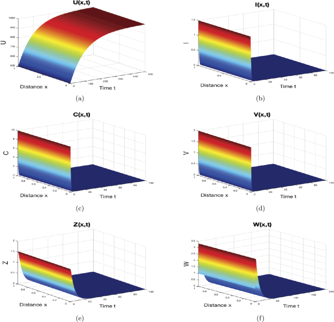

  

  The numerical simulations of system (44)–(46) when $R_{0}\leq1$. The infection-free equilibrium $M_{0}$ is globally asymptotically stable. The sub-figures show the spatiotemporal behaviors of (a) uninfected hepatocytes, (b) infected hepatocytes, (c) capsids, (d) viruses, (e) CTLs, and (f) B cells

• (ii) When $\gamma=0.5\text{ mm}^{3}\text{ virus}^{-1}\text{ day}^{-1}$, $p=0.01\text{ mm}^{3}\text{ cell}^{-1}\text{ day}^{-1}$, $\mu=1.5\text{ day}^{-1}$ and $\varsigma_{1}=0.02\text{ mm}^{3}\text{ cell}^{-1}$, then we find $0.5482=R_{1}<1<R_{0}=1.3889$ and $0.7569=R_{2}<1<R_{0}=1.3889$. For this set of parameters and according to Theorem 4, the solutions of system (44) converge to the immune-free equilibrium $M_{1}=(162.3944,13.9603,2.7921,0.4886,0,0)$ as shown in Fig. 2. The number of uninfected hepatocytes drops sharply when the HBV infection is chronic and the immune responses are not active.

  Figure 2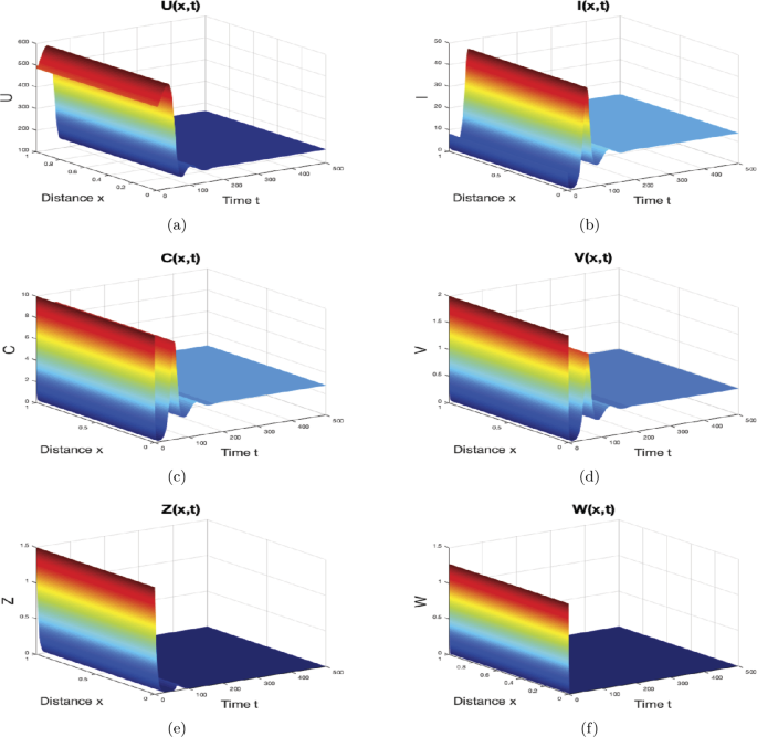

  

  The numerical simulations of system (44)–(46) when $R_{1}\leq1< R_{0}$ and $R_{2}\leq1< R_{0}$. The immune-free equilibrium $M_{1}$ is globally asymptotically stable. The sub-figures show the spatiotemporal behaviors of (a) uninfected hepatocytes, (b) infected hepatocytes, (c) capsids, (d) viruses, (e) CTLs, and (f) B cells

• (iii) We take $\gamma=0.5\text{ mm}^{3}\text{ virus}^{-1}\text{ day}^{-1}$, $p=0.01\text{ mm}^{3}\text{ cell}^{-1}\text{ day}^{-1}$, $\mu=0.5\text{ day}^{-1}$ and $\varsigma_{1}=0.02\text{ mm}^{3}\text{ cell}^{-1}$. These values give $R_{0}=1.3889>1$, $R_{1}=1.2023>1$, and $R_{3}=0.5725<1$. In agreement with the result of Theorem 5, the infection equilibrium $M_{2}=(313.1212,11.4516,2.2903,0.3334,0,1.7987)$ is globally asymptotically stable as can be observed from Fig. 3. Biologically, this case indicates that only B immune cells fight against HBV; as a result, the density of target cells has started to rise again after the sharp decline in the previous case. Moreover, the density of HBV is lower than its density in the previous case.

  Figure 3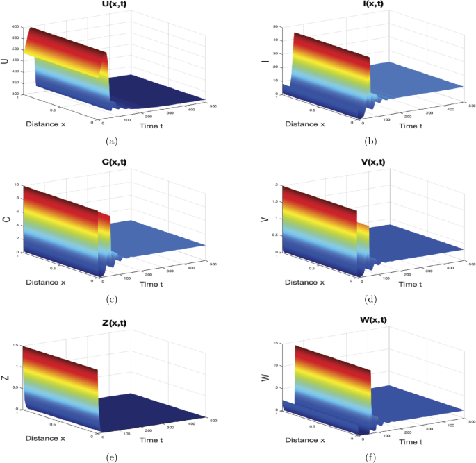

  

  The numerical simulations of system (44)–(46) when $R_{1}> 1$ and $R_{3}\leq1$. The infection equilibrium $M_{2}$ is globally asymptotically stable. The sub-figures show the spatiotemporal behaviors of (a) uninfected hepatocytes, (b) infected hepatocytes, (c) capsids, (d) viruses, (e) CTLs, and (f) B cells

• (iv) If $\gamma=0.5\text{ mm}^{3}\text{ virus}^{-1}\text{ day}^{-1}$, $p=0.07\text{ mm}^{3}\text{ cell}^{-1}\text{ day}^{-1}$, $\mu=0.5\text{ day}^{-1}$ and $\varsigma_{1}=0.01\text{ mm}^{3}\text{ cell}^{-1}$, then we obtain $R_{0}=2.6515>1$, $R_{2}=2.4515>1$, and $\frac {R_{1}}{R_{3}}=0.3<1$. For this choice of parameter values, the solutions of system (44) converge to the infection equilibrium $M_{3}=(579.4083,2.775,0.5546,0.097,0.8672,0)$, which supports Theorem 6. The results are shown in Fig. 4. In this situation, CTL immune response works alone to kill the infected cells which are the source of the virus.

  Figure 4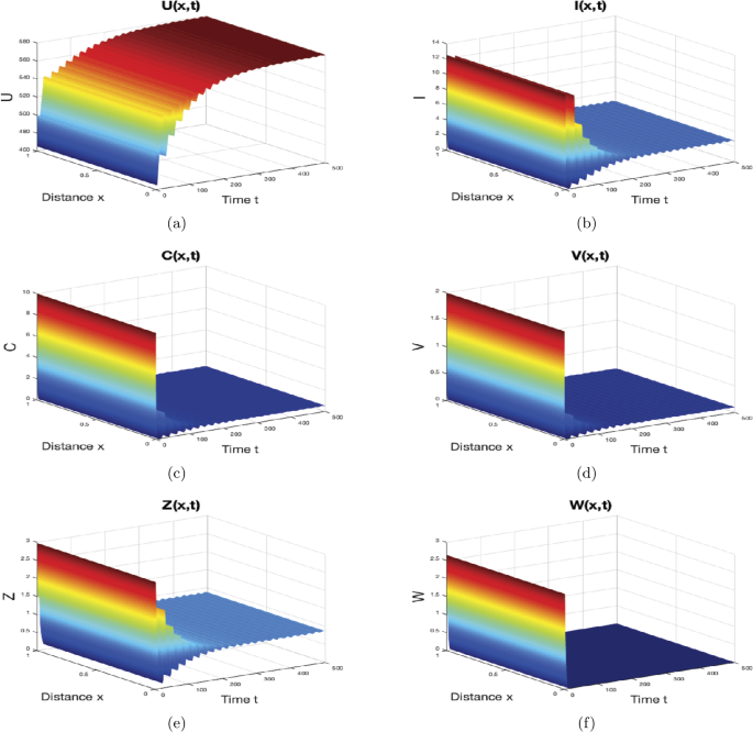

  

  The numerical simulations of system (44)–(46) when $R_{2}> 1$ and $\frac{R_{1}}{R_{3}}\leq1$. The infection equilibrium $M_{3}$ is globally asymptotically stable. The sub-figures show the spatiotemporal behaviors of (a) uninfected hepatocytes, (b) infected hepatocytes, (c) capsids, (d) viruses, (e) CTLs, and (f) B cells

• (v) When $\gamma=0.7\text{ mm}^{3}\text{ virus}^{-1}\text{ day}^{-1}$, $p=0.15\text{ mm}^{3}\text{ cell}^{-1}\text{ day}^{-1}$, $\mu=0.06\text{ day}^{-1}$ and $\varsigma_{1}=0.01\text{ mm}^{3} \text{ cell}^{-1}$, then we get $R_{0}=3.7121>1$, $R_{3}=3.0757>1$, $\frac{R_{1}}{R_{3}}=1.1667>1$. In agreement with Theorem 7, we can see from Fig. 5 that the equilibrium $M_{4}=(753.4535,1.3449,0.2708,0.0406,1.2688,1.5117)$ is globally asymptotically stable. Here, CTL and antibody immune responses work in parallel to kill the infected hepatocytes and attack the HBV, respectively. As a result, the number of healthy liver cells increases while the numbers of infected cells, capsids, and viruses decrease.

  Figure 5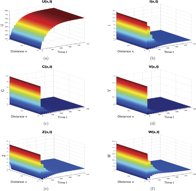

  

  The numerical simulations of system (44)–(46) when $R_{3}> 1$ and $R_{1}>R_{3}>1$. The equilibrium with two immune responses $M_{4}$ is globally asymptotically stable. The sub-figures show the spatiotemporal behaviors of (a) uninfected hepatocytes, (b) infected hepatocytes, (c) capsids, (d) viruses, (e) CTLs, and (f) B cells

6 Conclusion

In this paper, we have studied a diffusive HBV infection model with capsids and two forms of immune responses, the CTL and antibody immune responses. We have shown that the model has five equilibrium points which are given by the disease-free equilibrium $M_{0}$, the immune-free equilibrium $M_{1}$, the infection equilibrium with only antibody immune response $M_{2}$, the infection point with only CTL immune response $M_{3}$, and the equilibrium with both types of adaptive immunity $M_{4}$. The conditions for existence and global stability of these equilibrium points have produced four threshold parameters $R_{0}$, $R_{1}$, $R_{2}$, and $R_{3}$. The equilibrium point $M_{0}$ is globally asymptotically stable if $R_{0}\leq1$, which indicates that the liver cells are totally healthy and there is no infection. The equilibrium $M_{1}$ exists and is globally asymptotically stable if $R_{1}\leq1< R_{0}$ and $R_{2}\leq1< R_{0}$, and it reflects the situation when the immune responses have not been activated yet to counter the infection. The infection equilibrium $M_{2}$ exists and is globally asymptotically stable if $R_{1}>1$ and $R_{3}\leq1$, where only B lymphocytes work to defeat the virus. On the other hand, $M_{3}$ exists and is globally asymptotically stable equilibrium point if $R_{2}>1$ and $\frac{R_{1}}{R_{3}}\leq1$. In this case, only CTLs try to clear the infection by killing the infected hepatocytes. Finally, B and T immune cells work together to eliminate HBV infection at the equilibrium $M_{4}$ that exists and is globally asymptotically stable if $R_{1}>R_{3}>1$. The provided numerical simulations have supported the theoretical results and showed the spatiotemporal behavior of the solutions.

It is commonly observed that in viral infection processes, time delay is inevitable (see, e.g., [8,9,10,11, 44,45,46,47]). Extending model (2) to include the effect of treatments and time delays will give a deeper insight into HBV infection. Another extension of model (2) is to incorporate stochastic interactions (see [48]). We leave these points as future works.

References

Nowak, M.A., May, R.M.: Virus Dynamics: Mathematical Principles of Immunology and Virology. Oxford University Press, Oxford (2000)
World Health Organization: Global Hepatitis Report 2017. World Health Organization, Geneva (2017). License: CCBY-NC-SA 3.0 IGO
Pairan, A., Bruss, V.: Functional surfaces of the hepatitis B virus capsid. J. Virol. 83, 11616–11623 (2009)
Bruss, V.: Envelopment of the hepatitis B virus nucleocapsid. Virus Res. 106, 199–209 (2004)
Grimm, D., Thimme, R., Blum, H.E.: HBV life cycle and novel drug targets. Hepatol. Int. 5(2), 644–653 (2011)
Miao, H., Teng, Z., Abdurahman, X., Li, Z.: Global stability of a diffusive and delayed virus infection model with general incidence function and adaptive immune response. Comput. Appl. Math. 37(3), 3780–3805 (2018)
Nowak, M.A., Bangham, C.R.M.: Population dynamics of immune responses to persistent viruses. Science 272, 74–79 (1996)
Huang, G., Takeuchi, Y., Ma, W.: Lyapunov functionals for delay differential equations model of viral infections. SIAM J. Appl. Math. 70(7), 2693–2708 (2010)
Elaiw, A.M., Elnahary, E.Kh., Raezah, A.A.: Effect of cellular reservoirs and delays on the global dynamics of HIV. Adv. Differ. Equ. 2018, Article ID 85 (2018)
Hobiny, A.D., Elaiw, A.M., Almatrafi, A.: Stability of delayed pathogen dynamics models with latency and two routes of infection. Adv. Differ. Equ. 2018, Article ID 276 (2018)
Elaiw, A.M., Raezah, A.A., Azoz, S.A.: Stability of delayed HIV dynamics models with two latent reservoirs and immune impairment. Adv. Differ. Equ. 2018, Article ID 414 (2018)
Hattaf, K., Yousfi, N.: A generalized virus dynamics model with cell-to-cell transmission and cure rate. Adv. Differ. Equ. 2016, Article ID 174 (2016)
Elaiw, A.M., AlShamrani, N.H.: Stability of an adaptive immunity pathogen dynamics model with latency and multiple delays. Math. Methods Appl. Sci. 41(16), 6645–6672 (2018)
Shu, H., Wang, L., Watmough, J.: Global stability of a nonlinear viral infection model with infinitely distributed intracellular delays and CTL immune responses. SIAM J. Appl. Math. 73(3), 1280–1302 (2013)
Carvalho, A.R.M., Pinto, C.M.A., Baleanu, D.: HIV/HCV coinfection model: a fractional-order perspective for the effect of the HIV viral load. Adv. Differ. Equ. 2018, Article ID 2 (2018)
Elaiw, A.M., Almuallem, N.A.: Global properties of delayed-HIV dynamics models with differential drug efficacy in cocirculating target cells. Appl. Math. Comput. 265, 1067–1089 (2015)
Elaiw, A.M., AlShamrani, N.H.: Stability of a general adaptive immunity virus dynamics model with multi-stages of infected cells and two routes of infection. Math. Methods Appl. Sci. (2019). https://doi.org/10.1002/mma.5923
Elaiw, A.M., Alshaikh, M.A.: Stability analysis of a general discrete-time pathogen infection model with humoral immunity. J. Differ. Equ. Appl. (2019). https://doi.org/10.1080/10236198.2019.1662411
Huang, G., Ma, W., Takeuchi, Y.: Global properties for virus dynamics model with Beddington–DeAngelis functional response. Appl. Math. Lett. 22(11), 1690–1693 (2009)
Britton, N.F.: Essential Mathematical Biology. Springer, London (2003)
Wang, K., Wang, W.: Propagation of HBV with spatial dependence. Math. Biosci. 210, 78–95 (2007)
Gourley, S.A., So, J.W.H.: Dynamics of a food-limited population model incorporating nonlocal delays on a finite domain. J. Math. Biol. 44, 49–78 (2002)
Xu, R., Ma, Z.: An HBV model with diffusion and time delay. J. Theor. Biol. 257, 499–509 (2009)
Shaoli, W., Xinlong, F., Yinnian, H.: Global asymptotical properties for a diffused HBV infection model with CTL immune response and nonlinear incidence. Acta Math. Sci. 31B(5), 1959–1967 (2011)
Zhang, Y., Xu, Z.: Dynamics of a diffusive HBV model with delayed Beddington–DeAngelis response. Nonlinear Anal., Real World Appl. 15, 118–139 (2014)
Bellomo, N., Tao, Y.: Stabilization in a chemotaxis model for virus infection. Discrete Contin. Dyn. Syst., Ser. S 13(2), 105–117 (2020)
Geng, Y., Xu, J., Hou, J.: Discretization and dynamic consistency of a delayed and diffusive viral infection model. Appl. Math. Comput. 316, 282–295 (2018)
Manna, K., Chakrabarty, S.P.: Global stability and a non-standard finite difference scheme for a diffusion driven HBV model with capsids. J. Differ. Equ. Appl. 21(10), 918–933 (2015)
Guo, T., Liu, H., Xu, C., Yan, F.: Global stability of a diffusive and delayed HBV infection model with HBV DNA-containing capsids and general incidence rate. Discrete Contin. Dyn. Syst., Ser. B 23, 4223–4242 (2018)
Manna, K.: Dynamics of a delayed diffusive HBV infection model with capsids and CTL immune response. Int. J. Appl. Comput. Math. 4, Article ID 116 (2018). https://doi.org/10.1007/s40819-018-0552-4
Danane, J., Allali, K.: Mathematical analysis and treatment for a delayed hepatitis B viral infection model with the adaptive immune response and DNA-containing capsids. High-Throughput 7, Article ID 35 (2018). https://doi.org/10.3390/ht7040035
Xu, J., Geng, Y.: Threshold dynamics of a delayed virus infection model with cellular immunity and general nonlinear incidence. Math. Methods Appl. Sci. 42(3), 892–906 (2018)
Min, L., Su, Y., Kuang, Y.: Mathematical analysis of a basic virus infection model with application to HBV infection. Rocky Mt. J. Math. 38(5), 1573–1585 (2008)
Xu, Z., Xu, Y.: Stability of a CD4+ T cell viral infection model with diffusion. Int. J. Biomath. 11(5), Article ID 1850071 (2018)
Smith, H.L.: Monotone Dynamical Systems: An Introduction to the Theory of Competitive and Cooperative Systems. Am. Math. Soc., Providence (1995)
Protter, M.H., Weinberger, H.F.: Maximum Principles in Differential Equations. Prentice Hall, Englewood Cliffs (1967)
Henry, D.: Geometric Theory of Semilinear Parabolic Equations. Springer, New York (1993)
Hale, J.K., Verduyn Lunel, S.M.: Introduction to Functional Differential Equations. Springer, New York (1993)
Perelson, A., Kirschner, D., De Boer, R.: Dynamics of HIV infection of CD4+ T cells. Math. Biosci. 114(1), 81–125 (1993)
Culshaw, R., Ruan, S., Spiteri, R.: Optimal HIV treatment by maximising immune response. J. Math. Biol. 48(5), 545–562 (2004)
Pawelek, K., Liu, S., Pahlevani, F., Rong, L.: A model of HIV-1 infection with two time delays: mathematical analysis and comparison with patient data. Math. Biosci. 235(1), 98–109 (2012)
Beddington, J.R.: Mutual interference between parasites or predators and its effect on searching efficiency. J. Anim. Ecol. 44, 331–340 (1975)
DeAngelis, D.L., Goldstein, R.A., O’Neill, R.V.: A model for tropic interaction. Ecology 56, 881–892 (1975)
Elaiw, A.M., Elnahary, E.Kh.: Analysis of general humoral immunity HIV dynamics model with HAART and distributed delays. Mathematics 7, Article ID 157 (2019)
Elaiw, A.M., Almatrafi, A., Hobiny, A.D., Hattaf, K.: Global properties of a general latent pathogen dynamics model with delayed pathogenic and cellular infections. Discrete Dyn. Nat. Soc. 2019, Article ID 9585497 (2019)
Elaiw, A.M., Raezah, A.A.: Stability of general virus dynamics models with both cellular and viral infections and delays. Math. Methods Appl. Sci. 40(16), 5863–5880 (2017)
Elaiw, A.M., Alshehaiween, S.F., Hobiny, A.D.: Global properties of delay-distributed HIV dynamics model including impairment of B-cell functions. Mathematics 7, Article ID 837 (2019)
Gibelli, L., Elaiw, A., Alghamdi, M.A., Althiabi, A.M.: Heterogeneous population dynamics of active particles: progression, mutations, and selection dynamics. Math. Models Methods Appl. Sci. 27, 617–640 (2017)
Acknowledgements
This project funded by the Deanship of Scientific Research (DSR), King Abdulaziz University, Jeddah, under grant No. (DF-005-130-1441). The authors, therefore, gratefully acknowledge DSR technical and financial support.
Availability of data and materials
Not applicable.
Funding
Author information
Authors and Affiliations
Contributions
All authors contributed equally to the writing of this paper. All authors read and approved the final manuscript.
Corresponding author
Ethics declarations
Competing interests
The authors declare that they have no competing interests.
Additional information
Publisher’s Note
Springer Nature remains neutral with regard to jurisdictional claims in published maps and institutional affiliations.
Rights and permissions
Open Access This article is licensed under a Creative Commons Attribution 4.0 International License, which permits use, sharing, adaptation, distribution and reproduction in any medium or format, as long as you give appropriate credit to the original author(s) and the source, provide a link to the Creative Commons licence, and indicate if changes were made. The images or other third party material in this article are included in the article’s Creative Commons licence, unless indicated otherwise in a credit line to the material. If material is not included in the article’s Creative Commons licence and your intended use is not permitted by statutory regulation or exceeds the permitted use, you will need to obtain permission directly from the copyright holder. To view a copy of this licence, visit http://creativecommons.org/licenses/by/4.0/.
About this article
Cite this article
Elaiw, A.M., Al Agha, A.D. Global dynamics of a general diffusive HBV infection model with capsids and adaptive immune response. Adv Differ Equ 2019, 519 (2019). https://doi.org/10.1186/s13662-019-2448-y
Received:
Accepted:
Published:
DOI: https://doi.org/10.1186/s13662-019-2448-y