
Abstract
In this research work, a mathematical model related to HIV-I cure infection therapy consisting of three populations is investigated from the fractional calculus viewpoint. Fractional version of the model under consideration has been proposed. The proposed model is examined by using the Atangana–Baleanu fractional operator in the Caputo sense (ABC). The theory of Picard–Lindelöf has been employed to prove existence and uniqueness of the special solutions of the proposed fractional-order model. Further, it is also shown that the non-negative hyper-plane \(\mathbb{R}_{+}^{3}\) is a positively invariant region for the underlying model. Finally, to analyze the results, some numerical simulations are carried out via a numerical technique recently devised for finding approximate solutions of fractional-order dynamical systems. Upon comparison of the numerical simulations, it has been demonstrated that the proposed fractional-order model is more accurate than its classical version. All the necessary computations have been performed using MATLAB R2018a with double precision arithmetic.
1 Introduction
Human immunodeficiency virus (HIV) is the virus that is responsible for acquired immunodeficiency syndrome (AIDS). It relies upon the transcription and translation machinery of its host cell. The virus infects a specific type of cell in the human immune system known as CD4 helper lymphocyte cells (CD4+ T). These cells are destroyed by HIV thereby making it harder for the body to fight other infections. When the level of the CD4+ T cells declines beneath a critical level, cell-mediated immunity is lost and the body becomes progressively susceptible to infections, resulting in the development of AIDS as explained in various studies [1,2,3,4,5]. Finding a cure for AIDS still happens to be one of the greatest challenges for scientists globally. In order to understand the dynamics of this deadly infection, various mathematical models have been suggested and modified. These models have provided vital information about the information of the interactions of distinct constituents, including infected cells and immune system, and have thus improved the progress in understanding the HIV-1 infection [6]. This may bestow towards proper enhancement of new drugs and for designing optimal combination of existing cures. In this regard, a classical mathematical model, that is, a model based upon first-order ordinary differential equations, has recently been discussed in [7, 8]. This classical model is non-linear and autonomous in nature, presented as follows:
with the initial conditions \(X(0)=X_{0} \geq 0\), \(Y(t)=Y_{0}(t) \geq 0\), \(V(0)=V_{0}(t) \geq 0\), where \(X(t)\) denotes the density of the uninfected cells, \(Y(t)\) represents the density of infected cells, and \(V(t)\) is density of the virus (HIV-I). Apart from these three populations, there are six working parameters in the model which play important role in understanding the dynamics of the model. The parameter λ represents the rate at which new susceptible cell is produced, σ is the natural death rate of uninfected cells, β is the rate of infection, a is the death rate of infected cells which produce new virus particles, k is the rate at which new viruses are produced, and p is the clearance rate of the virus. Table 1 shows their estimated values.
Fractional-order operators have successfully been applied to model a number of mathematical problems arising from the fields like physics, chemistry, biology, ecology, finance, and engineering. Many such mathematical models have been proposed and analyzed by using different fractional-order operators as can be found in the recent studies [9,10,11,12,13,14,15,16,17,18,19,20,21,22,23,24,25,26]. It is well known that Riemann–Liouville and Caputo-type fractional operators have singular type of kernels in the integrands of their definitions. Therefore, in order to tackle the physical problems with singularity, Atangana and Baleanu proposed a new operator based upon the Mittag-Leffler type kernel [27]. The proposed operators have all the features of the operator known as the Caputo and Fabrizio (CF) operator as introduced in [28], and the kernel introduced is non-local and non-singular. Recent studies in numerical and analytical techniques of non-local kernel are getting much attention of researchers around the globe exploring this field. One of the main advantages of this operator is its useful application in the modeling of biological dynamical systems. Various biological systems have been proposed and analyzed by using the operator devised by Atangana–Baleanu in the Caputo sense (ABC).
Although, some other fractional models of HIV do exist, the main purpose of this research study is to expand the study of the model under consideration (1) by replacing its classical derivative with the ABC operator [27]. In this way, a new mathematical model related to the HIV-I infection is proposed in the present research study. Later, with the help of Picard–Lindelöf theory, we prove the existence and uniqueness of some special solutions of the proposed fractional-order model under the ABC operator. Finally, numerical simulations are carried out to illustrate the behavior of the solutions of the proposed model using a newly devised numerical scheme in [29]. It may also be noted at this stage that the stability analysis along with computation of the reproductive number \(\mathcal{R}\) regarding the integer-order model (1) has been discussed in [8], and for the sake of brevity such analysis is not repeated in the present research study.
The structure of the present paper is as follows. Some basic definitions and theorems necessary to comprehend the rest of the analysis are presented in Sect. 2 followed by Sect. 3 which consists of the proposed fractional-order model with its brief discussion. Section 4 provides, while using the Picard–Lindelöf theory, the discussion to understand the existence of the solutions for the proposed fractional-order model, whereas the uniqueness and the positivity of its solutions is also proved in the same section. This is followed by Sect. 5 which presents a newly devised numerical technique to approximate the fractional-order dynamical systems under the ABC operator. Numerical simulations are provided in Sect. 6 with graphical illustrations to help us understand the dynamics of the model. Finally, the paper ends with Sect. 7 by discussing major contributions made in the present research work.
2 Preliminaries
In this piece of the section, we present some definitions and properties of the ABC operator [27].
Definition 1
([27])
Let \(f\in K'(b,d)\), \(d>c\), \(\varOmega \in [0,1]\), the Atangana–Baleanu operator in the Caputo sense (ABC) can be defined as follows:
where \(F(\varOmega )\) is a normalized function satisfying \(F(0)=F(1)=1\).
Definition 2
([27])
Consider \(f\in K'(b,d)\), \(d>b\), \(\varOmega \in [0,1]\), which may not be differentiable, the AB fractional operator in the Riemann–Liouville (ABR) sense can be represented by
Definition 3
([27])
Atangana–Baleanu integral of the function \(f(t)\) having order \(\varOmega >0\) is defined by the following equation:
It may be noted if \(\varOmega \rightarrow 1\) then the classical integral is retrieved.
2.1 Important properties
The above presented definitions have been utilized to model numerous applications in biological fields. In order to understand and use these practical definitions, it is important to revisit their fundamental properties [27]:
and
Theorem 1
Let f be continuous on the closed interval \([b, d]\) with b, \(d \mathbb{R}\). The following identity exists on \([b, d]\):
where \(\lVert f(x) \rVert =\sup_{b \le x \le d}|f(x)|\).
Theorem 2
Let \(f(t)\) and \(g(t)\) be two continuous functions. The following Lipschitz condition is satisfied:
and
Theorem 3
([27])
The following fractional-order ordinary differential equation
has the unique solution given as follows:
Theorem 4
Let \(h(z) \in C[0, T]\) for sufficiently large T and \({}^{\mathrm{ABC}}D _{0,t}^{\varOmega }h(t) \in (0, T]\), then
with \(0 \leq s \leq t\), \(\forall t \in (0, T]\).
Corollary 1
Consider that \(h(z) \in C[0, T]\) and \({}^{\mathrm{ABC}}D_{0,t}^{\varOmega }h(t) \in (0, T]\), where \(\varOmega \in (0, 1]\). Then, if
-
i.
\({}^{\mathrm{ABC}}D_{0,t}^{\varOmega } h(z) \geq 0\), \(\forall z \in (0, T)\), then \(h(z)\) is non-decreasing.
-
ii.
\({}^{\mathrm{ABC}}D_{0,t}^{\varOmega } h(z) \leq 0\), \(\forall z \in (0, T)\), then \(h(z)\) is non-increasing.
3 Fractional-order HIV-I model
The classical model (1) does not take into account the effects of memory (history) to analyze the spread of the HIV virus in much detail. To analyze the model under such effects, the model has been modified, and a new model having fractional-order derivatives with the ABC operator has been proposed as follows:
with the initial conditions \(X(0)=X_{0} \geq 0\), \(Y(0)=Y_{0} \geq 0\), \(V(0)=V _{0} \geq 0\), where all the working parameters are defined as in the classical model (1) presented above.
4 Mathematical analysis for the solutions
4.1 Existence of the solutions
In this piece of the section, the existence of the special solutions of the proposed fractional-order model (13) is proved with the help of the Picard–Lindelöf theorem [30].
Let \(P = K(q)\times (q)\) and \(K(q)\) be a Banach space of a real-valued continuous function \(R \rightarrow R\) on q with the norm \(\lVert X,Y,V \rVert = \lVert X \rVert + \lVert Y \rVert + \lVert V \rVert \), where \(\lVert X \rVert =\sup\{|X(t)|:t \in q\}\), \(\lVert Y \rVert =\sup\{|Y(t)|:t \in q\}\), and \(\lVert V \rVert =\sup\{|V(t)|:t \in q\}\).
The ordinary differential equation (10) with a prescribed initial condition can be converted to write in terms of the Volterra integral equation of the second type as follows:
For the sake of brevity, we introduce some new notations as follows:
Theorem 5
These kernels \(K_{1}\), \(K_{2}\), and \(K_{3}\) satisfy the Lipschitz condition if the following inequalities are valid on them:
Proof
We begin the analysis with the kernel \(K_{1}(t,X)\). Let X and \(X_{1}\) be two functions such that
where \(\sigma _{1} ={\sigma + \beta s}\) and \(s=\sup_{t \in V(t)} \lVert V(t) \rVert \). Then \(K_{1}\) satisfies the Lipschitz condition, and when \(0 \le \sigma _{1} < 1\), one may observe that it is also a contraction for \(K_{1}\).
In the same way, we consider the kernel \(K_{2}(t,Y)\). Let Y and \(Y_{1}\) be two functions such that
where \(\sigma _{2} =a\). Then the kernel \(K_{2}\) also satisfies the Lipschitz condition, and when \(0 \le \sigma _{2} < 1\), one can see that it is also a contraction for \(K_{2}\).
Finally, we consider the kernel \(K_{3}(t,V)\). Let V and \(V_{1}\) be two functions such that
where \(\sigma _{3} =p\). Then the Lipschitz condition is satisfied for the kernel \(K_{3}\). For \(0 \le \sigma _{3} < 1\), one can see that it is also a contraction for \(K_{3}\).
Thus, using the kernels, one obtains
Considering the following recursive formula, one obtains
with the initial conditions
The difference between the successive components is given by
These simplifications yield the following structure:
Applying the norm condition for (28), one obtains
Since the Lipschitz condition is satisfied by the kernels, one obtains the following:
Thus,
Similarly, one can obtain the following:
□
Theorem 6
The HIV-I model has a unique solution on the condition that the term \(t_{\mathrm{max}}\) satisfies the following inequality:
Proof
It has been demonstrated above that the functions \(X(t)\), \(Y(t)\), and \(V(t)\) are bounded and the Lipschitz condition is also satisfied by each of their kernels. Therefore, using the recursive method and equations (35)–(37), one obtains the following:
Hence, the obtained solutions exist and are smooth. Next, it is shown that these solutions are in fact special solutions of the proposed fractional-order model (13). Consider that
The basic aim is to demonstrate that at infinity \(\lVert B_{ \infty } \rVert \rightarrow 0\), \(\lVert C_{\infty } \rVert \rightarrow 0\), and \(\lVert D_{\infty } \rVert \rightarrow 0\). Therefore, starting from the first case, we get the following:
Applying the process recursively, one obtains the following:
Then at \(t_{\mathrm{max}}\), one obtains the following:
Taking the limit \(n\rightarrow \infty \), we get \(\lVert B_{ \infty } \rVert \rightarrow 0\). Continuing in the same way, one can show that \(\lVert C_{\infty } \rVert \rightarrow 0\) and \(\lVert D_{\infty } \rVert \rightarrow 0\). □
4.2 Uniqueness of the special solutions
The uniqueness for the solutions of the proposed fractional-order model (13) is established in this part of the section. To start with, suppose that there exist other solutions for each equation of the proposed fractional-order model (13), say \(X_{1}(t)\), \(Y_{1}(t)\), and \(V_{1}(t)\), respectively. Considering the first equation, one obtains
Applying the norm condition on (32), one obtains
This yields the following:
This yields
Thus, it has been proved that the special solutions of the proposed fractional-order model (13) are unique. Following the same steps, it is easy to show the uniqueness of the remaining two functions, that is, \(Y(t)\) and \(V(t)\).
4.3 Positivity of the solutions
To show the positivity of the solutions of the model, that is, the non-negative hyper-plane \(\mathbb{R}_{+}^{3}\) is a positively invariant region for model (13), consider the following:
Furthermore,
It is demonstrated that on each hyper-plane bounding the non-negative hyper-plane, the vector field points into \(\mathbb{R}_{+}^{3}\). Using the proposed fractional-order model (13), one obtains the following:
Hence, from Corollary 1, it is observed that the solutions of the proposed fractional-order model (13) will be in \(\mathbb{R}_{+}^{3}\). With this, we complete the proof for the positivity of the solutions of the underlying model.
5 Numerical technique
The proposed fractional-order model (13) is non-linear in nature leading to possibility of having no closed form solution. It is, therefore, necessary to deal with it numerically. Recently, a numerical technique based upon the ABC operator has been devised to solve such dynamical systems in [29]. Given below is the structure of the technique to be used to serve the purpose in the present research work. Consider the following initial value problem in fractional-order settings under the ABC operator:
Problem (54) can also written as
At the point \(t = t_{n+1}\), \(n = 0, 1, 2 ,\ldots\) . The above equation can be written as
Consider \(f(\mu , y(\mu ))\) using a two-step Lagrange polynomial, one obtains the following relation on \([t_{k}, t_{k+1}]\):
Again, considering equation (55) for \(f(\mu , y(\mu ))\), one obtains
Simplifications yield the following:
where \(J_{n}^{\varOmega }\) n is the remainder term obtained as
6 Numerical simulations
Using the AB fractional-order integral for the proposed fractional-order model (13) with the kernels \(K_{j}\), \(j = 1, 2, 3\), the following structure is obtained:
subject to the following initial conditions:
Using the numerical technique at a point \(t=t_{n+1}\), one obtains
where \({}^{j}J_{n}^{\varOmega }\), \(j = 1, 2, 3\) are the remainder terms represented by the relations [29]:
Since not only the proposed fractional-order model but the classical HIV-I model is also non-linear, so it carries the possibility of having no closed form solution in all cases. Therefore the classical version of the model has been solved using the standard Runge–Kutta fourth-order method from standard numerical analysis with time step-size \(h=10^{-4}\), whereas the fractional model is dealt with equations (63)–(65) using the non-negative initial conditions with the time step-size \(h=10^{-2}\). Simulations given in Figs. 1–6 reveal the past or memory behavior for the numerical solutions of the proposed fractional-order model under the ABC operator. Before eventually reaching the solution curve of the classical HIV-I model, it has various shapes that speak for the past behavior of the underlying system, and this is something that cannot be obtained via classical mathematical models. Hence, this justifies the fact that fractional-order models estimate the real or experimental data more efficiently than their classical counterparts in most physical and natural phenomena such as the one presented in this research study. The values of the working parameters used in the present numerical simulations are listed in Table 1. Numerical simulations obtained in the tables and figures are summarized as follows:
-
On the basis of the parameters from Table 1, the graphical simulation results have shown that when the initial amount of density of the virus is not present, then the density of the uninfected cells decreases for the starting four units of time and then starts to increase; but eventually, after 35 units of time, it gets the stabilization as shown in Figs. 1–2 in contrast to Figs. 3–4 wherein such a stabilization becomes evident after about 20 units of time for the density of infected cells.
Figure 1 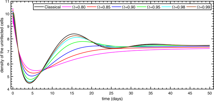
Density of the uninfected cells with initial conditions \(X(0)=10\), \(Y(0)=10\), \(V(0)=0\) for \(t \in [0, 50]\)
Figure 2 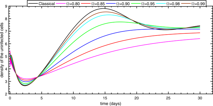
Density of the uninfected cells with initial conditions \(X(0)=5\), \(Y(0)=20\), \(V(0)=0\) for \(t \in [0, 30]\)
Figure 3 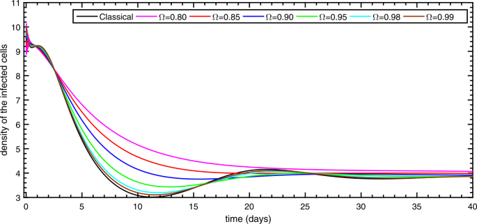
Density of the infected cells with initial conditions \(X(0)=10\), \(Y(0)=10\), \(V(0)=0\) for \(t \in [0, 40]\)
Figure 4 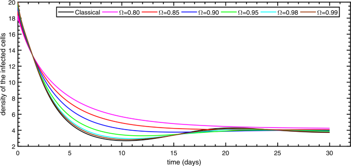
Density of the infected cells with initial conditions \(X(0)=5\), \(Y(0)=20\), \(V(0)=0\) for \(t \in [0, 30]\)
-
Similar sort of trend appears in the case with no initial density of virus in Fig. 5, but when initially there is some amount of initial density of virus present in the system, then the system gets stabilized after a longer period of time as shown in Fig. 6.
Figure 5 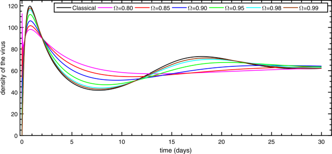
Density of the virus \(X(0)=1\), \(Y(0)=10\), \(V(0)=0\) for \(t \in [0, 30]\)
Figure 6 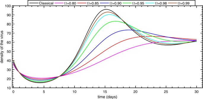
Density of the virus with initial conditions \(X(0)=1\), \(Y(0)=2\), \(V(0)=40\) for \(t \in [0, 30]\)
-
Looking at the tabular data, it is observed that when initially there is some amount of density of the virus \(V(0)=40\) and there is no production of new virus \(k=0\), then density of the virus starts to vanish but is not completely wiped out due to the presence of β value, and this real behavior is clearly depicted in Table 2 for the fractional-order parameter \(\varOmega =0.99\).
Table 2 Approximate solutions using RK4 (first row) and numerical technique (59) (second row, \(\varOmega = 0.99\)) with step-size \(h=10^{-3}\) over \([0, 10]\) for \(X(0)=1\), \(Y(0)=2\), \(V(0)=40\) having parameter \(k=0\) -
Table 3 suggests that for no initial presence of the virus but with clearance rate \(p=0\), the density of the virus increases at a lower rate than the classical case \(\varOmega =1\), whereas the density of uninfected and infected cells increases at a faster rate.
Table 3 Approximate solutions using RK4 (first row) and numerical technique (59) (second row, \(\varOmega = 0.99\)) with step-size \(h=10^{-3}\) over \([0, 10]\) for \(X(0)=10\), \(Y(0)=10\), \(V(0)=0\) having parameters \(k=5\), \(p=0\) -
Finally, the doubling of the clearance rate \(p=6\) for the fractional-order parameter \(\varOmega =0.98\) in Table 4 leads to slowing down the virus production, which is obvious in the real situations.
Table 4 Approximate solutions using RK4 (first row) and numerical technique (59) (second row, \(\varOmega = 0.98\)) with step-size \(h=10^{-3}\) over \([0, 10]\) for \(X(0)=Y(0)=V(0)=20\) having parameter \(p=6\)


7 Concluding remarks
It has been shown in the present study that the proposed fractional-order HIV-I model is capable of capturing all those memory effects which are not possible to obtain via a classical version of the model. Being a non-linear system, the special solution of the HIV-I model has been guaranteed through existence and uniqueness theorems carried out via Picard–Lindelöf theory. During the analysis of the proposed model, it has been observed that the fractional-order model gives the entire history for the solution of the system (HIV-I) under consideration and is thus capable of predicting the experimental data more accurately. This is due to an essential feature of the fractional-order operators called the non-locality which makes them more suitable for memory-dependent dynamical systems. It is this non-locality that provides us an infinite number of degrees of freedom for the fractional-order parameter \(\varOmega >0\).
References
Douek, D.C., Roederer, M., Koup, R.A.: Emerging concepts in the immunopathogenesis of AIDS. Annu. Rev. Med. 60, 471–484 (2009)
Buonomo, B., Vargas-De-Leon, C.: Global stability for an HIV-I infection model including an eclipse stage of infected cells. J. Math. Anal. Appl. 385, 709–720 (2012)
Perelson, A.S., Kirschner, D.E., De Boer, R.: Dynamics of HIV infection of CD4+ T cells. Math. Biosci. 114, 81–125 (1993)
Perelson, A.S., Neumann, A.U., Markowitz, M., Leonard, J.M., Ho, D.D.: HIV-1 dynamics in vivo: virion clearance rate, infected cell life-span, and viral generation time. Science 271, 1582–1586 (1996)
Perelson, A.S., Nelson, P.W.: Mathematical analysis of HIV-1 dynamics in vivo. J. Soc. Ind. Appl. Math. 41, 3–44 (1999)
Tian, Y., Liu, X.: Global dynamics of a virus dynamical model with general incidence rate and cure rate. Nonlinear Anal., Real World Appl. 16, 17–26 (2014)
Ali, N., Zaman, G., Abdullah, Alqahtani, A.M., Alshomrani, A.S.: The effects of time lag and cure rate on the global dynamics of HIV-I model. BioMed Res. Int. 2017, Article ID 8094947 (2017). https://doi.org/10.1155/2017/8094947
Jones, E., Roemer, P., Raghupathi, M., Pankavich, S.: Analysis and simulation of the three-component model of HIV dynamics (2013). arXiv:1312.3671
Yusuf, A., Qureshi, S., Inc, M., Aliyu, A.I., Baleanu, D., Shaikh, A.A.: Two-strain epidemic model involving fractional derivative with Mittag-Leffler kernel. Chaos, Interdiscip. J. Nonlinear Sci. 28, 123121 (2018)
Koca, I.: Modelling the spread of Ebola virus with Atangana–Baleanu fractional operators. Eur. Phys. J. Plus 133, 100 (2018)
Singh, J., Kumar, D., Hammouch, Z., Atangana, A.: A fractional epidemiological model for computer viruses pertaining to a new fractional derivative. Appl. Math. Comput. 316, 504–515 (2018)
Ullah, S., Khan, M.A., Farooq, M.: A fractional model for the dynamics of TB virus. Chaos Solitons Fractals 116, 63–71 (2018)
Sheikh, N.A., Ali, F., Khan, I., Saqib, M.: A modern approach of Caputo–Fabrizio time-fractional derivative to MHD free convection flow of generalized second-grade fluid in a porous medium. Neural Comput. Appl. 306, 1865–1875 (2018)
Jajarmi, A., Baleanu, D.: A new fractional analysis on the interaction of HIV with CD4+ T-cells. Chaos Solitons Fractals 113, 221–229 (2018)
Abro, K.A., Memon, A.A., Memon, A.A.: Functionality of circuit via modern fractional differentiations. Analog Integr. Circuits Signal Process. 99, 11–21 (2019)
Abro, K.A., Memon, A.A., Uqaili, M.A.: A comparative mathematical analysis of RL and RC electrical circuits via Atangana–Baleanu and Caputo–Fabrizio fractional derivatives. Eur. Phys. J. Plus 133, 113 (2018)
Arshad, S., Baleanu, D., Bu, W., Tang, Y.: Effects of HIV infection on CD4+ T-cell population based on a fractional-order model. Adv. Differ. Equ. 2017, 92 (2017)
Almeida, R., Bastos, N.R.O., Monteiro, M.T.T.: Modeling some real phenomena by fractional differential equations. Math. Methods Appl. Sci. 39, 4846–4855 (2016)
Diethelm, K.: A fractional calculus based model for the simulation of an outbreak of dengue fever. Nonlinear Dyn. 71, 613–619 (2013)
Mohammad, F., Moradi, L., Baleanu, D., Jajarmi, A.: A hybrid functions numerical scheme for fractional optimal control problems: application to non-analytic dynamical systems. J. Vib. Control 24, 5030–5043 (2018)
Baleanu, D., Sajjadi, S.S., Jajarmi, A., Asad, J.H.: New features of the fractional Euler–Lagrange equations for a physical system within non-singular derivative operator. Eur. Phys. J. Plus 134, 181 (2019)
Baleanu, D., Jajarmi, A., Asad, J.H.: Classical and fractional aspects of two coupled pendulums. Rom. Rep. Phys. 71, 103 (2019)
Atangana, A., Gomez-Aguilar, J.F.: Decolonisation of fractional calculus rules: breaking commutativity and associativity to capture more natural phenomena. Eur. Phys. J. Plus 133, 166 (2018)
Atangana, A.: Non validity of index law in fractional calculus: a fractional differential operator with Markovian and non-Markovian properties. Phys. A, Stat. Mech. Appl. 505, 688–706 (2018)
Atangana, A., Gomez-Aguilar, J.F.: Fractional derivatives with no-index law property: application to chaos and statistics. Chaos Solitons Fractals 114, 516–535 (2018)
Atangana, A.: Blind in a commutative world: simple illustrations with functions and chaotic attractors. Chaos Solitons Fractals 114, 347–363 (2018)
Atangana, A., Baleanu, D.: New fractional derivative with non-local and non-singular kernel theory and application to heat transfer model. Therm. Sci. 20, 763–769 (2016)
Caputo, M., Mauro, F.: A new definition of fractional derivative without singular kernel. Prog. Fract. Differ. Appl. 1(2), 73–85 (2015)
Toufik, M., Atangana, A.: New numerical approximation of fractional derivative with non-local and non-singular kernel: application to chaotic models. Eur. Phys. J. Plus 132, 444 (2017)
Nevanlinna, O.: Remarks on Picard–Lindelöf iteration. BIT Numer. Math. 29, 535–562 (1989)
Acknowledgements
The authors would like to thank the referees for their important comments and remarks.
Availability of data and materials
Not applicable.
Funding
This work was supported by the National Natural Science Foundation of China (Grant No. 11571378).
Author information
Authors and Affiliations
Contributions
The authors contributed equally to the writing of this paper. All authors approved the final version of the manuscript.
Corresponding author
Ethics declarations
Competing interests
The authors declare that they have no competing interests.
Additional information
Publisher’s Note
Springer Nature remains neutral with regard to jurisdictional claims in published maps and institutional affiliations.
Rights and permissions
Open Access This article is distributed under the terms of the Creative Commons Attribution 4.0 International License (http://creativecommons.org/licenses/by/4.0/), which permits unrestricted use, distribution, and reproduction in any medium, provided you give appropriate credit to the original author(s) and the source, provide a link to the Creative Commons license, and indicate if changes were made.
About this article

Cite this article
Aliyu, A.I., Alshomrani, A.S., Li, Y. et al. Existence theory and numerical simulation of HIV-I cure model with new fractional derivative possessing a non-singular kernel. Adv Differ Equ 2019, 408 (2019). https://doi.org/10.1186/s13662-019-2336-5
Received:
Accepted:
Published:
DOI: https://doi.org/10.1186/s13662-019-2336-5