
Abstract
In this paper, a new generalized exponential rational function method is employed to extract new solitary wave solutions for the Zakharov–Kuznetsov equation (ZKE). The ZKE exhibits the behavior of weakly nonlinear ion-acoustic waves in incorporated hot isothermal electrons and cold ions in the presence of a uniform magnetic field. Furthermore, the stability for the governing equations is investigated via the aspect of linear stability analysis. Numerical simulations are made to shed light on the characteristics of the obtained solutions.
1 Introduction
Nonlinear evolution equations (NLEEs) have been very important aspects owing to their very wide range of applicability in nonlinear science. In science nonlinear physical phenomena are one of the most significant areas of study and they appear in various fields of science and engineering, such as plasma physics, fluid mechanics, gas dynamics, elasticity, relativity, chemical reactions, ecology, optical fiber, solid state physics, biomechanics, to mention few. All these equations are fundamentally controlled by NLEEs [1,2,3,4,5,6]. NLEEs are often used to illustrate the motion of separated waves. Ever since the arrival of solitary wave in scientific work, it has been getting more concentration. Thus, it is vital to extract exact traveling wave solutions to NLEEs. This is because obtaining exact solutions to NLEEs gives us the liberty to present information on the characteristics of a complex physical phenomenon. Thus, the construction of exact traveling wave solutions to NLEEs has become a priority in the analysis of nonlinear physical phenomenon. A lot of analytical approaches have been used to establish traveling wave solutions for NLEEs [7,8,9,10,11,12,13]. On solitons, nonlinear physical phenomena and other novel solutions of NLEEs, there has been a variety of theoretical work [14,15,16,17,18,19,20,21,22,23,24].
Moreover, it is well known that stability analysis (SA) is very important in the investigation of integrability, internal properties, existence and uniqueness of a differential equation [14,15,16,17]. In this paper, new traveling wave solutions using a relatively new technique, namely the new generalized exponential rational function method (GERFM) [25] and stability analysis via the concept of linear stability analysis are constructed for the \((2+1)\)-dimensional ZK equation given by [26,27,28,29,30,31]
where μ and δ are nonzero arbitrary constants and \(\phi=\phi(x,y,t)\). \(\phi(x,y,t)\) is for the electrostatic wave potential in plasmas, that is, a function of the spatial variables x, y and the temporal variable t. The ZK equation determines the behavior of weakly nonlinear ion-acoustic waves incorporating hot isothermal electrons and cold ions in the presence of a uniform magnetic field [32,33,34,35,36,37]. The ZK equation also involves an anisotropic two-dimensional generalization of the KdV equation and can be analyzed in magnetized plasma for a tiny amplitude Alfvén wave at a critical angle to the uninterrupted magnetic field [32,33,34,35,36,37]. There has not been a lot of studies on this special form (1.1) of the ZK equation in the literature. The main aim of the current work is to establish new solutions to this less studied equation by means of GERFM.
2 Description of the GERFM
The GERFM may be described as follows [25]:
Step 1. Surmise that there is a nonlinear partial differential equation express by
Applying \(\psi=\psi(\xi)\) along with \(\xi= kx+my-\omega t\), we obtain
where \(k, m\) and ω are constants that will be computed later.
Step 2. Next, we surmise that Eq. (2.2) has the formal solution
where \(p_{1},p_{2},p_{3},p_{4}\), and \(q_{1},q_{2},q_{3},q_{4}\) represent the complex (or real) numbers provided that Eq. (2.1) is written as
Meanwhile the coefficients \(A_{0}, A_{k}, B_{k}(1 \leq k \leq N)\) and \(p_{n}, q_{n}(1 \leq n \leq4)\) will be obtained such that (2.4) satisfies (2.2). In addition, N is a positive integer that can be obtained by applying the homogeneous balance principle.
Step 3. Plugging (2.4) into Eq. (2.2) and organizing all terms yield the polynomial equation \(P(e^{q_{1} \xi},e^{q_{2} \xi},e^{q_{3} \xi},e^{q_{4} \xi})=0\). Equating every coefficient of P to zero, a set of algebraic equations for \(p_{n}, q_{n}(1 \leq n \leq4)\), and \(k, m, \omega, A_{0},A_{1},B_{1}\) will be derived with the help of Maple.
Step 4. Solving the outcomes in Step 3 and then putting non-trivial solutions in (2.4), we obtain the soliton solutions of Eq. (1.1).
3 Application of GERFM to ZK
In order to construct explicit traveling wave solutions to Eq. (1.1), we propose the following traveling wave transformation:
Applying Eq. (3.1) to Eq. (1.1) and integrating once with respect to ξ yield
Applying the balance principle to the terms of \(u^{2}\) and \(u''\) in Eq. (3.2) gives \(2N=N+2\) so \(N=2\). So (2.4) will turn into
where \(\varPhi(\xi)\) is giving by (2.3). Substituting (3.3) into (3.2) and, following the method described in Sect. 2, we obtain non-trivial solutions of (1.1) as follows.
Family 1: For \(p=[ i, -i,1,1]\) and \(q=[i,-i,i,-i]\), (2.3) turns into
-
Case 1:
$$\begin{aligned} &k=k,\qquad m=-{\frac{ \sqrt{6}\sqrt{6 {k}^{2}+\mu B_{{2}}}}{6 \sqrt{-\delta-1}}},\qquad \omega=\frac{4}{3} \mu kB_{{2}}, \\ &A_{{0}}=2 B_{{2}},\qquad A_{{1} }=0,\qquad A_{{2}}=B_{{2}},\qquad B_{{1}}=0,\qquad B_{{2}}=B_{{2}} . \end{aligned}$$
Putting these results in Eqs. (3.3) and (3.4), the exact solution of Eq. (1.1) is obtained:
$$\phi_{1} (x,y,t ) = {\frac{B_{{2}}}{ \cos^{2} ( \xi ) \sin^{2} ( \xi ) }} , $$where, for \(\delta<-1\), we have
$$\xi= k x -{\frac{ \sqrt{6}\sqrt{6 {k}^{2}+\mu B_{{2}}}}{6 \sqrt{-\delta-1}}} y - \frac{4}{3} \mu kB_{{2}} t. $$ -
Case 2:
$$\begin{aligned} &k=k,\qquad m=-{\frac{ \sqrt{2}\sqrt{2 {k}^{3}-\omega}}{2\sqrt{k }\sqrt{-\delta-1}}},\qquad \omega=\omega,\qquad A_{{0}}=-{ \frac{\omega}{k\mu}},\\ & A_{{ 1}}=0,\qquad A_{{2}}=- { \frac{3\omega}{k\mu}},\qquad B_{{1}}=0,\qquad B_{{2}}=0 . \end{aligned}$$
Putting these results in Eqs. (3.3) and (3.4), the exact solution of Eq. (1.1) is obtained:
$$\phi_{2} (x,y,t )= {\frac{ ( 2 \cos^{2} ( \xi ) -3 ) \omega}{ k\mu\cos^{2} ( \xi ) }} , $$where, for \(\delta<-1\), we have
$$\xi= k x -{\frac{ \sqrt{2}\sqrt{2 {k}^{3}-\omega}}{2\sqrt{k }\sqrt{-\delta-1}}} y - \omega t. $$ -
Case 3:
$$\begin{aligned} &k=k,\qquad m=-{\frac{ \sqrt{6}\sqrt{6 {k}^{2}+\mu B_{{2}}}}{6 \sqrt{-\delta-1}}},\qquad \omega=-\frac{1}{3} \mu kB_{{2}}, \\ &A_{{0}}=\frac{1}{3} B_{{2}},\qquad A_{ {1}}=0,\qquad A_{{2}}=0,\qquad B_{{1}}=0,\qquad B_{{2}}=B_{{2}} . \end{aligned}$$
Putting these results in Eqs. (3.3) and (3.4), the exact solution of Eq. (1.1) is obtained:
$$\phi_{3} (x,y,t )= {\frac{ ( 2 \cos^{2} ( \xi ) + 1 ) B_{{2}}}{ 3 \sin^{2} ( \xi ) }} , $$where, for \(\delta<-1\), we have
$$\xi= k x -{\frac{ \sqrt{6}\sqrt{6 {k}^{2}+\mu B_{{2}}}}{6 \sqrt{-\delta-1}}},\qquad \omega=-\frac{1}{3} \mu kB_{{2}} y +\frac{1}{3} \mu kB_{{2}} t. $$ -
Case 4:
$$\begin{aligned} &k=k,\qquad m=-{\frac{ \sqrt{2}\sqrt{2 {k}^{3}+\omega}}{2\sqrt{k }\sqrt{-\delta-1}}},\qquad \omega=\omega,\qquad A_{{0}}={\frac{3 \omega}{k\mu}}, \\ &A_{{1}}=0,\qquad A_{{2}}={\frac{3 \omega}{k\mu}},\qquad B_{{1}}=0,\qquad B_{{2}}=0 . \end{aligned}$$
Putting these results in Eqs. (3.3) and (3.4), the exact solution of Eq. (1.1) is obtained:
$$\phi_{4} (x,y,t )= {\frac{3 \omega}{k\mu \cos^{2} ( \xi ) }} , $$where, for \(\delta<-1\), we have
$$\xi= k x -{\frac{ \sqrt{2}\sqrt{2 {k}^{3}+\omega}}{2\sqrt{k }\sqrt{-\delta-1}}} y - \omega t. $$
Family 2: For \(p=[1+i,1-i,1,1]\) and \(q=[i,-i,i,-i]\), (2.3) turns into
-
Case 1:
$$\begin{aligned} &k=k,\qquad m=-{\frac{ \sqrt{3}\sqrt{12 {k}^{2}-A_{{1}}\mu}}{6 \sqrt{-\delta-1}}},\qquad \omega=\frac{1}{ 6} \mu kA_{{1}}, \\ &A_{{0}}=-\frac{2}{3} A_{{1}},\qquad A_{ {1}}=A_{{1}},\qquad A_{{2}}=- \frac{1}{2} A_{{1}},\qquad B_{{1}}=0,\qquad B_{{2}}=0 . \end{aligned}$$
Putting these results in Eqs. (3.3) and (3.5), the exact solution of Eq. (1.1) is obtained:
$$\phi_{5} (x,y,t )= {\frac{ ( 2 \cos^{2} ( \xi ) - 3 ) A_{{1}}}{6 \cos^{2} ( \xi ) }} , $$where, for \(\delta<-1\), we have
$$\xi= k x -{\frac{ \sqrt{3}\sqrt{12 {k}^{2}-A_{{1}}\mu}}{6 \sqrt{-\delta-1}}} y - \frac{1}{ 6} \mu kA_{{1}} t. $$ -
Case 2:
$$\begin{aligned} &k=k,\qquad m=-{\frac{ \sqrt{2}\sqrt{2 {k}^{3}+\omega}}{2\sqrt{k }\sqrt{-\delta-1}}},\qquad\omega=\omega, \\ &A_{{0}}={\frac{6 \omega}{k\mu}},\qquad A_{{1}}=0,\qquad A_{{2}}=0,\qquad B_{{1}}=-{ \frac{12 \omega}{k\mu}},\qquad B_{{2}}={ \frac{12 \omega}{k\mu}} . \end{aligned}$$
Putting these results in Eqs. (3.3) and (3.5), the exact solution of Eq. (1.1) is obtained:
$$\phi_{6} (x,y,t )= -{\frac{6 \omega}{k\mu ( 2 \sin ( \xi ) \cos ( \xi ) -1 ) }} , $$where, for \(\delta<-1\), we have
$$\xi= k x -{\frac{ \sqrt{2}\sqrt{2 {k}^{3}+\omega}}{2\sqrt{k }\sqrt{-\delta-1}}} y - \omega t. $$ -
Case 3:
$$\begin{aligned} &k=k,\qquad m=-{\frac{ \sqrt{2}\sqrt{2 {k}^{3}-\omega}}{2\sqrt{k }\sqrt{-\delta-1}}},\qquad \omega=\omega, \\ &A_{{0}}=-{\frac{4 \omega}{k\mu}},\qquad A _{{1}}=0,\qquad A_{{2}}=0,\qquad B_{{1}}={ \frac{12 \omega}{k\mu}},\qquad B_{{2}}=-{ \frac{12 \omega}{k\mu}} . \end{aligned}$$
Putting these results in Eqs. (3.3) and (3.5), the exact solution of Eq. (1.1) is obtained:
$$\phi_{7} (x,y,t )= {\frac{4 \omega ( \sin ( \xi ) \cos ( \xi ) +1 ) }{k\mu ( 2 \sin ( \xi ) \cos ( \xi ) -1 ) }} , $$where, for \(\delta<-1\), we have
$$\xi= k x -{\frac{ \sqrt{2}\sqrt{2 {k}^{3}-\omega}}{2\sqrt{k }\sqrt{-\delta-1}}} y - \omega t. $$
Family 3: For \(p=[1,-1,1,1]\) and \(q=[-1,1,-1,1]\), (2.3) turns into
-
Case 1:
$$\begin{aligned} &k=\frac{1}{ 6} \sqrt{-6 \mu A_{{2}}-36 ( \delta+1 ) { m}^{2}},\qquad m=m,\\ & \omega=-\frac{2}{9} \mu A_{{2}}\sqrt{-6 \mu A_{{2}}-36 ( \delta+1 ) {m}^{2}}, \\ &A_{{0}}=-2 A_{{2}},\qquad A_{{1}}=0,\qquad A_{{2} }=A_{{2}},\qquad B_{{1}}=0,\qquad B_{{2}}=A_{{2}} . \end{aligned}$$
Putting these results in Eqs. (3.3) and (3.6), the exact solution of Eq. (1.1) is obtained:
$$\phi_{8} (x,y,t )= {\frac{A_{{2}}}{ \cosh^{2} ( \xi ) \sinh^{2} ( \xi ) }} , $$where
$$\xi= \frac{1}{ 6} \sqrt{-6 \mu A_{{2}}-36 ( \delta+1 ) { m}^{2}} x + m y +\frac{2}{9} \mu A_{{2}}\sqrt{-6 \mu A_{{2}}-36 ( \delta+1 ) {m}^{2}} t. $$ -
Case 2:
$$\begin{aligned} &k=\frac{1}{ 6} \sqrt{-6 \mu B_{{2}}-36 ( \delta+1 ) { m}^{2}},\qquad m=m,\\ & \omega=\frac{1}{18} \sqrt{-6 \mu B_{{2}}-36 ( \delta+1 ) {m}^{2}}\mu B_{{2}}, \\ &A_{{0}}=-\frac{1}{3} B_{{2}},\qquad A_{{1}}=0,\qquad A_{{2}}=0 ,\qquad B_{{1}}=0,\qquad B_{{2}}=B_{{2}} . \end{aligned}$$
Putting these results in Eqs. (3.3) and (3.6), the exact solution of Eq. (1.1) is obtained:
$$\phi_{9} (x,y,t )= - {\frac{B_{{2}} ( \tanh^{2} ( \xi ) -3 ) }{ 3 \tanh^{ 2} ( \xi ) }} , $$where
$$\xi= \frac{1}{ 6} \sqrt{-6 \mu B_{{2}}-36 ( \delta+1 ) { m}^{2}} x + m y - \frac{1}{18} \sqrt{-6 \mu B_{{2}}-36 ( \delta+1 ) {m}^{2}}\mu B_{{2}} t. $$ -
Case 3:
$$\begin{aligned} &k=\frac{1}{ 6} \sqrt{-6 \mu B_{{2}}-36 ( \delta+1 ) { m}^{2}},\qquad m=m,\\ & \omega=-\frac{1}{18} \sqrt{-6 \mu B_{{2}}-36 ( \delta+1 ) {m}^{2}}\mu B_{{2}}, \\ &A_{{0}}=-B_{{2}},\qquad A_{{1}}=0,\qquad A_{{2}}=0,\qquad B_{ {1}}=0,\qquad B_{{2}}=B_{{2}} . \end{aligned}$$
Putting these results in Eqs. (3.3) and (3.7), the exact solution of Eq. (1.1) is obtained:
$$\phi_{10} (x,y,t )= {\frac{B_{{2}}}{ \sinh^{2} ( \xi ) }} , $$where
$$\xi= \frac{1}{ 6} \sqrt{-6 \mu B_{{2}}-36 ( \delta+1 ) { m}^{2}} x + m y +\frac{1}{18} \sqrt{-6 \mu B_{{2}}-36 ( \delta+1 ) {m}^{2}}\mu B_{{2}} t. $$
Family 4: For \(p=[-2,-3,1,1]\) and \(q=[1,0,1,0]\), (2.3) turns into
-
Case 1:
$$\begin{aligned} &k=k,\qquad m=-{\frac{ \sqrt{6}\sqrt{6 {k}^{2}+\mu A_{{2}}}}{6 \sqrt{-\delta- 1}}},\qquad \omega=\frac{1}{12} \mu kA_{{2}}, \\ &A_{{0}}={\frac{37 A_{{ 2}}}{6}},\qquad A_{{1}}=5 A_{{2}},\qquad A_{{2}}=A_{{2}},\qquad B_{{1}}=0,\qquad B_{{2}}=0 . \end{aligned}$$
Putting these results in Eqs. (3.3) and (3.7), the exact solution of Eq. (1.1) is obtained:
$$\phi_{11} (x,y,t )= - {\frac{A_{{2}} ( -{\mathrm{ e}^{2 \xi}}+4 {\mathrm{ e}^{\xi}}-1 ) }{ 6 ( 1+{\mathrm{ e}^{\xi}} ) ^{2}}} , $$where, for \(\delta<-1\), we have
$$\xi= k x -{\frac{ \sqrt{6}\sqrt{6 {k}^{2}+\mu A_{{2}}}}{6 \sqrt{-\delta- 1}}} y - \frac{1}{12} \mu kA_{{2}} t. $$ -
Case 2:
$$\begin{aligned} &k=k,\qquad m=-{\frac{ \sqrt{{k}^{3}-2 \omega}}{\sqrt{k}\sqrt{ -\delta-1}}},\qquad\omega=\omega, \\ &A_{{0}}=-{\frac{72 \omega}{\mu k}},\qquad A_{{1} }=0,\qquad A_{{2}}=0,\qquad B_{{1}}=-{ \frac{360 \omega}{\mu k}},\qquad B_{{2}}=-{ \frac{432 \omega}{\mu k}} . \end{aligned}$$
Putting these results in Eqs. (3.3) and (3.7), the exact solution of Eq. (1.1) is obtained:
$$\phi_{12} (x,y,t )= {\frac{72 \omega{\mathrm{ e}^{\xi}}}{\mu k ( 2 {\mathrm{ e}^{\xi}}+ 3 ) ^{2}}} , $$where, for \(\delta<-1\), we have
$$\xi= k x -{\frac{ \sqrt{{k}^{3}-2 \omega}}{\sqrt{k}\sqrt{ -\delta-1}}} y - \omega t. $$
Family 5: For \(p=[-3,-1,1,1]\) and \(q=[1,-1,1,-1]\), (2.3) turns into
-
Case 1:
$$\begin{aligned} &k=k,\qquad m=-{\frac{ \sqrt{2}\sqrt{2 {k}^{3}-\omega}}{2\sqrt{k }\sqrt{-\delta-1}}},\qquad\omega=\omega, \\ &A_{{0}}=-{\frac{9 \omega}{\mu k}} ,\qquad A_{{1}}=0,\qquad A_{{2}}=0,\qquad B_{{1}}=-{ \frac{36 \omega}{\mu k}},\qquad B_{{2}}=- {\frac{27 \omega}{\mu k}} . \end{aligned}$$
Putting these results in Eqs. (3.3) and (3.8), the exact solution of Eq. (1.1) is obtained:
$$\phi_{13} (x,y,t )= {\frac{ 9 \omega}{k\mu ( 5 \cosh^{2} ( \xi ) +4 \cosh ( \xi ) \sinh ( \xi ) -1 ) }} , $$where, for \(\delta<-1\), we have
$$\xi= k x -{\frac{ \sqrt{2}\sqrt{2 {k}^{3}-\omega}}{2\sqrt{k }\sqrt{-\delta-1}}} y - \omega t. $$ -
Case 2:
$$\begin{aligned} &k=k,\qquad m=-{\frac{ \sqrt{2}\sqrt{2 {k}^{3}+\omega}}{2\sqrt{k }\sqrt{-\delta-1}}},\qquad \omega=\omega, \\ &A_{{0}}={\frac{11 \omega}{\mu k}} ,\qquad A_{{1}}=0,\qquad A_{{2}}=0,\qquad B_{{1}}={ \frac{36 \omega}{\mu k}},\qquad B_{{2}}= {\frac{27 \omega}{\mu k}} . \end{aligned}$$
Putting these results in Eqs. (3.3) and (3.8), the exact solution of Eq. (1.1) is obtained:
$$\phi_{14} (x,y,t )= {\frac{\omega ( 18 \cosh^{4} ( \xi ) -33 \cosh^{2} ( \xi ) +36 \cosh ( \xi ) \sinh ( \xi ) +11 ) }{k\mu ( 3 \cosh^{2} ( \xi ) +1 ) ^{ 2}}} , $$where, for \(\delta<-1\), we have
$$\xi= k x -{\frac{ \sqrt{2}\sqrt{2 {k}^{3}+\omega}}{2\sqrt{k }\sqrt{-\delta-1}}} y - \omega t. $$
Family 6: For \(p=[1,1,1,-1]\) and \(q=[1,-1,1,-1]\), (2.3) turns into
-
Case 1:
$$\begin{aligned} & k=\frac{1}{ 6} \sqrt{-6 \mu A_{{2}}-36 ( \delta+1 ) { m}^{2}},\qquad m=m,\\ & \omega=\frac{2}{9} \mu A_{{2}}\sqrt{-6 \mu A_{{2}}-36 ( \delta+1 ) {m}^{2}}, \\ &A_{{0}}=\frac{2}{3} A_{{2}},\qquad A_{{1}}=0,\qquad A_{{2 }}=A_{{2}},\qquad B_{{1}}=0,\qquad B_{{2}}=A_{{2}} . \end{aligned}$$
Putting these results in Eqs. (3.3) and (3.9), the exact solution of Eq. (1.1) is obtained:
$$\phi_{15} (x,y,t )= {\frac{A_{{2}} ( 3 \operatorname{coth}^{4} (\xi ) +2 \operatorname{coth}^{2} (\xi ) +3 ) }{ {3} \operatorname{coth} ^{2} (\xi ) }} , $$where, for \(\delta<-1\), we have
$$\xi= \frac{1}{ 6} \sqrt{-6 \mu A_{{2}}-36 ( \delta+1 ) { m}^{2}} x + m y - \frac{2}{9} \mu A_{{2}}\sqrt{-6 \mu A_{{2}}-36 ( \delta+1 ) {m}^{2}} t. $$ -
Case 2:
$$\begin{aligned} &k=k,\qquad m=-{\frac{ \sqrt{2}\sqrt{2 {k}^{3}-\omega}}{2\sqrt{k }\sqrt{-\delta-1}}},\qquad\omega=\omega, \\ &A_{{0}}={\frac{3 \omega}{k\mu}},\qquad A_{{1}}=0,\qquad A_{{2}}=0,\qquad B_{{1}}=0,\qquad B_{{2}}=-{ \frac{3 \omega}{k\mu}} . \end{aligned}$$
Putting these results in Eqs. (3.3) and (3.9), the exact solution of Eq. (1.1) is obtained:
$$\phi_{16} (x,y,t )= {\frac{3 \omega}{k\mu\cosh^{2} ( \xi ) } } , $$where, for \(\delta<-1\), we have
$$\xi= k x -{\frac{ \sqrt{2}\sqrt{2 {k}^{3}-\omega}}{2\sqrt{k }\sqrt{-\delta-1}}} y - \omega t. $$
Family 7: For \(p=[-2,-1,1,1]\), \(q=[0,1,0,1]\), and \(r=[0,0]\), (2.3) turns into
-
Case 1:
$$\begin{aligned} &k=k,\qquad m=-{\frac{ \sqrt{{k}^{3}+2 \omega}}{\sqrt{k}\sqrt{ -\delta-1}}},\qquad \omega=\omega, \\ &A_{{0}}={\frac{26 \omega}{k\mu}},\qquad A_{{1}}=0 ,\qquad A_{{2}}=0,\qquad B_{{1}}={ \frac{72 \omega}{k\mu}},\qquad B_{{2}}={\frac{48 \omega}{k\mu}} . \end{aligned}$$
Putting these results in Eqs. (3.3) and (3.10), the exact solution of Eq. (1.1) is obtained:
$$\phi_{17} (x,y,t )= {\frac{2 \omega ( {\mathrm{ e}^{2 \xi}}-8 {\mathrm{ e}^{\xi}}+4 ) }{k\mu ( {\mathrm{ e}^{\xi}}+2 ) ^{2}}} , $$where, for \(\delta<-1\), we have
$$\xi= k x -{\frac{ \sqrt{{k}^{3}+2 \omega}}{\sqrt{k}\sqrt{ -\delta-1}}} y - \omega t. $$ -
Case 2:
$$\begin{aligned} &k=k,\qquad m=-{\frac{ \sqrt{{k}^{3}-2 \omega}}{\sqrt{k}\sqrt{ - \delta-1}}},\qquad \omega=\omega, \\ &A_{{0}}=-{\frac{24 \omega}{k\mu}},\qquad A_{{1}}=0 ,\qquad A_{{2}}=0,\qquad B_{{1}}=-{ \frac{72 \omega}{k\mu}},\qquad B_{{2}}=-{\frac{48 \omega}{k\mu}} . \end{aligned}$$
Putting these results in Eqs. (3.3) and (3.10), the exact solution of Eq. (1.1) is obtained:
$$\phi_{18} (x,y,t )= {\frac{24 \omega{\mathrm{ e}^{\xi}}}{k\mu ( {\mathrm{ e}^{\xi}}+2 ) ^{2}}} , $$where, for \(\delta<-1\), we have
$$\xi= k x -{\frac{ \sqrt{{k}^{3}-2 \omega}}{\sqrt{k}\sqrt{ - \delta-1}}} y - \omega t. $$
Family 8: For \(p=[2,0,-1,1]\) and \(q=[-1,0,-1,1]\), (2.3) turns into
-
Case 1:
$$\begin{aligned} &k=k,\qquad m=-{\frac{ \sqrt{6}\sqrt{6 {k}^{2}+\mu A_{{2}}}}{6 \sqrt{-\delta-1}}},\qquad \omega=\frac{1}{3} \mu kA_{{2}}, \\ &A_{{0}}=\frac{2}{3} A_{{2}},\qquad A_{{ 1}}=-2 A_{{2}},\qquad A_{{2}}=A_{{2}},\qquad B_{{1}}=0,\qquad B_{{2}}=0 . \end{aligned}$$
Putting these results in Eqs. (3.3) and (3.11), the exact solution of Eq. (1.1) is obtained:
$$\phi_{19} (x,y,t )= {\frac{ ( 2 \cosh^{2} ( \xi ) -3 ) A_{{2}}}{3 \cosh^{2} ( \xi ) }} , $$where, for \(\delta<-1\), we have
$$\xi= k x -{\frac{ \sqrt{6}\sqrt{6 {k}^{2}+\mu A_{{2}}}}{6 \sqrt{-\delta-1}}} y - \frac{1}{3} \mu kA_{{2}} t. $$
Family 9: For \(p=[2,0,1,-1]\) and \(q=[1,0,i,-i]\), (2.3) turns into
-
Case 1:
$$\begin{aligned} &k=k,\qquad m=-{\frac{ \sqrt{6}\sqrt{6 {k}^{2}+\mu A_{{2}}}}{6 \sqrt{-\delta-1}}},\qquad \omega=-\frac{1}{3} \mu kA_{{2}}, \\ &A_{{0}}=\frac{4}{3} A_{{2}},\qquad A_{ {1}}=2 A_{{2}},\qquad A_{{2}}=A_{{2}},\qquad B_{{1}}=0,\qquad B_{{2}}=0 . \end{aligned}$$
Putting these results in Eqs. (3.3) and (3.12), the exact solution of Eq. (1.1) is obtained:
$$\phi_{20} (x,y,t )= {\frac{ ( 2 \cos^{2} ( \xi ) + 1 ) A_{{2}}}{3 \sin^{2} ( \xi ) }} , $$where, for \(\delta<-1\), we have
$$\xi= k x -{\frac{ \sqrt{6}\sqrt{6 {k}^{2}+\mu A_{{2}}}}{6 \sqrt{-\delta-1}}} y +\frac{1}{3} \mu kA_{{2}} t. $$
Family 10: For \(p=[1+i,1-i,1,1]\), \(q=[-i,i,-i,i]\), and \(r=[0,0]\), (2.3) turns into
-
Case 1:
$$\begin{aligned} &k=k,\qquad m=-{\frac{ \sqrt{6}\sqrt{6 {k}^{2}+\mu A_{{2}}}}{6 \sqrt{-\delta-1}}},\qquad \omega=\frac{1}{3} \mu kA_{{2}}, \\ &A_{{0}}=\frac{2}{3} A_{{2}},\qquad A_{{ 1}}=-2 A_{{2}},\qquad A_{{2}}=A_{{2}},\qquad B_{{1}}=0,\qquad B_{{2}}=0 . \end{aligned}$$
Putting these results in Eqs. (3.3) and (3.13), the exact solution of Eq. (1.1) is obtained and the physical features of some of the solutions are depicted in Figs. 1 to 5:
$$\phi_{21} (x,y,t )= {\frac{ ( 2 \cosh^{2} ( \xi ) +1 ) A_{{2}}}{ 3 \sinh^{2} ( \xi ) }} , $$where, for \(\delta<-1\), we have
$$\xi= k x -{\frac{ \sqrt{6}\sqrt{6 {k}^{2}+\mu A_{{2}}}}{6 \sqrt{-\delta-1}}} y - \frac{1}{3} \mu kA_{{2}} t. $$Figure 1 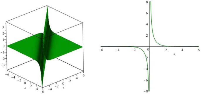
3D plot for \(\phi_{8}\) at \(y=1\) with \(A_{2}=\mu=\delta=1\) and 2D at \(t=0\)
Figure 2 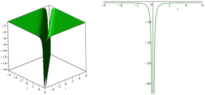
3D plot for \(\phi_{8}\) at \(y=1\) with \(B_{2}=\mu=\delta=1\) and 2D at \(t=0\)
Figure 3 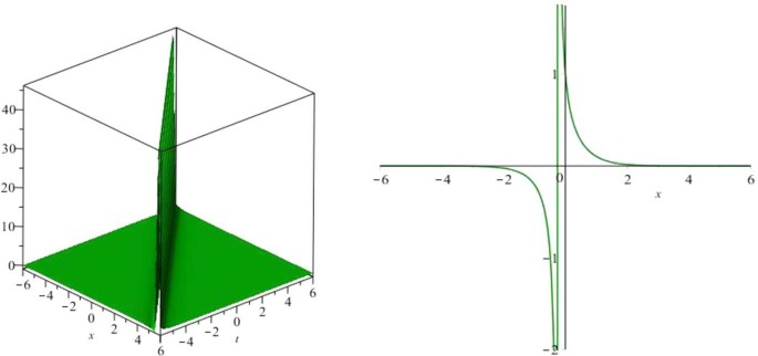
3D plot for \(\phi_{13}\) at \(y=1\) with \(\sigma=\mu=k=\delta=1\) and 2D at \(t=0\)
Figure 4 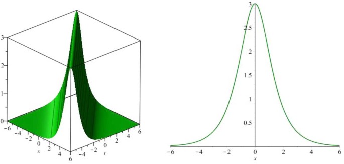
3D plot for \(\phi_{16}\) at \(y=1\) with \(\sigma=\mu=k=\delta=1\) and 2D at \(t=0\)
Figure 5 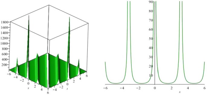
3D plot for \(\phi_{20}\) at \(y=1\) with \(A_{2}=k=\delta=1\) and 2D at \(t=0\)


4 Stability analysis of Eq. (1.1)
The connection for the dispersion in Eq. (1.1) will be analyzed [14,15,16,17]. The features of the real part (Re) of σ show whether the outcome will become larger or disappear in a given period. When the real part of \(\sigma(k)\) is negative for every k values, the superposition of solutions of the form \(e^{(i\sigma t + ikx)}\) may subsequently disappear. Put differently, if the the real part is positive for some values of k, some components of a superposition will subsequently become huge. The former is regarded as the stable case, while the latter is regarded as the unstable case. Furthermore, if the maximum of the real part is zero, the case is regarded to be the marginally stable case. It is burdensome to evaluate the long term behavior in this case. Moreover, in Fig. 6 we plot frequency of the pertubation against the wave number.

Frequency of the perturbation against the wave number when \(P_{0}<0\) and \(P_{0}>0\), respectively
Consider the perturbed solution of the form
It is easy to see that any constant \(P_{0}\) is a steady state solution of Eq. (1.1). Inserting Eq. (4.1) into Eq. (1.1), one gets
linearizing (4.2) in ϵ gives
Suppose that Eq. (4.3) has a solution of the form
where k is the normalized wave number; substituting Eq. (4.4) into Eq. (4.3), we get
Solving for σ from the above equation yields
From Eq. (4.5), one can see that the real part is negative for all k values, then any superposition of the solutions will appear to decay. Therefore, the dispersion is stable.
5 Conclusion
This research applied GERFM to extracting new solitary wave solutions for the ZK equation. The ZK equation exhibits the behavior of weakly nonlinear ion-acoustic waves incorporating hot isothermal electrons and cold ions in the presence of a uniform magnetic field. There have not been a lot of studies on this special form (1.1) of the ZK equation in the literature. Owing to this, it is of great importance to establish different types of solutions to this equation. We successfully obtained solutions such as exact solutions, exact periodic wave solutions, soliton solutions and exponential function solutions. GERFM has the capacity to generate several types of solutions in different form unlike some of the classic methods that could only generate a small number of solutions. Thus, GERFM is very efficient and effective in extracting new types of solutions to varieties of NLEEs. Graphical features of some of the obtained solutions are presented in order to shed more light on the characteristics of the obtained solutions. Furthermore, the stability of the governing equations was investigated via a linear stability analysis.
References
Ablowitz, M.J., Clarkson, P.A.: Solitons, Nonlinear Evolution Equations and Inverse Scattering Transform. Cambridge University Press, Cambridge (1990)
Tchier, F., Aliyu, A.I., Yusuf, A., Inc, M.: Dynamics of solitons to the ill-posed Boussinesq equation. Eur. Phys. J. Plus 132, 136 (2017)
Tchier, F., Yusuf, A., Aliyu, A.I., Inc, M.: Soliton solutions and conservation laws for lossy nonlinear transmission line equation. Superlattices Microstruct. 107, 320 (2017)
Ma, W.X.: A soliton hierarchy associated with so(3,R). Appl. Math. Comput. 220, 117 (2013)
Dodd, R., Eilbeck, J., Gibbon, J., Morris, H.: Solitons and Nonlinear Wave Equations. Academic Press, San Diego (1988)
Zabusky, N.: A Synergetic Approach to Problems of Nonlinear Dispersive Wave Propagation and Interaction. Academic Press, San Diego (1967)
He, J.H.: Application of homotopy perturbation method to nonlinear wave equations. Chaos Solitons Fractals 26(3), 695–700 (2005)
He, J.H.: Variational principles for some nonlinear partial differential equations with variable coefficients. Chaos Solitons Fractals 19, 4 (2004)
Adomian, G.: Solving Frontier Problems of Physics: The Decomposition Method. Kluwer Academic Publishers, Boston (1994)
Khan, K., Akbar, M.A.: Exact and solitary wave solutions for the Tzitzeica–Dodd–Bullough and the modified KdV–Zakharov–Kuznetsov equations using the modified simple equation method. Ain Shams Eng. J. 4(4), 903–909 (2013)
Khan, K., Akbar, M.A.: Traveling wave solutions of the \((2+1)\)-dimensional Zoomeron equation and the Burgers equations via the MSE method and the Exp-function method. Ain Shams Eng. J. 5(1), 247–256 (2014)
Bekir, A., Boz, A.: Exact solutions for nonlinear evolution equation using Exp-function method. Phys. Lett. A 372, 1619–1625 (2008)
Roshid, H.O., Rahman, N., Akbar, M.A.: Traveling waves solutions of nonlinear Klein Gordon equation by extended (G/G)-expansion method. Ann. Pure Appl. Math. 3, 10–16 (2013)
Osman, M.S., Korkmaz, A., Rezazadeh, H., Mirzazadeh, M., Eslami, M., Zhou, Q.: The unified method for conformable time fractional Schrodinger equation with perturbation terms. Chin. J. Phys.. 56(5), 2500–2506 (2018)
Korkmaz, A.: Complex wave solutions to mathematical biology models I: Newell–Whitehead–Segel and Zeldovich equations. J. Comput. Nonlinear Dyn. 13(8), 081004 (2017)
Rezazadeh, H., Korkmaz, A., Eslami, M., Vahidi, J., Asghari, R.: Travelling wave solution of conformable fractional generalized reaction Duffing model by generalized projective Riccati equation method. Opt. Quantum Electron. 50(150), 1–13 (2018)
Korkmaz, A., Hosseini, K.: Exact solutions of a nonlinear conformable time fractional parabolic equation with exponential nonlinearity using reliable methods. Opt. Quantum Electron. 49(278), 1–10 (2017)
Liu, W., Liu, M., Han, H., Fang, S., Teng, H., Lei, M., Wei, Z.: Nonlinear optical properties of WSe2 and MoSe2 films and their applications in passively Q-switched erbium doped fiber lasers. Photo. Res. 6(10), C15–C21 (2018)
Liu, M., OuYang, Y., Hou, H., Lei, M., Liu, W., Wei, Z.: MoS2 saturable absorber prepared by chemical vapor deposition method for nonlinear control in Q-switching fiber laser. Chin. Phys. B 27(8), 084211 (2018)
Liu, W., Liu, M., OuYang, Y., Hou, H., Lei, M., Wei, Z.: CVD-grown MoSe2 with high modulation depth for ultrafast mode-locked erbium-doped fiber laser. Nanotechnology 29(39), 394002 (2018)
Zhang, Y., Yang, C., Yu, W., Mirzazadeh, M., Zhou, Q., Liu, W.: Interactions of vector anti-dark solitons for the coupled nonlinear Schrödinger equation in inhomogeneous fibers. Nonlinear Dyn. 94, 1351–1360 (2018)
Liu, X., Triki, H., Zhou, Q., Liu, W., Biswas, A.: Analytic study on interactions between periodic solitons with controllable parameters. Nonlinear Dyn. 94, 703–709 (2018)
Yu, W., Ekici, M., Mirzazadeh, M., Zhou, Q., Liu, W.: Periodic oscillations of dark solitons in nonlinear optics. Optik 165, 341–344 (2018)
Guo, H., Zhang, X., Ma, G., Zhang, X., Yang, C., Zhou, Q., Liu, W.: Analytic study on interactions of some types of solitary waves. Optik 164, 132–137 (2018)
Ghanbari, B., Inc, M.: A new generalized exponential rational function method to find exact special solutions for the resonance nonlinear Schrödinger equation. Eur. Phys. J. Plus 133, 1–19 (2018)
Wazwaz, A.M.: The extended tanh method for the Zakharov–Kuznetsov (ZK) equation, the modified ZK equation, and its generalized forms. Commun. Nonlinear Sci. Numer. Simul. 13, 1039 (2008)
Ma, H.-C., Yu, Y.-D., Ge, D.-J.: The auxiliary equation method for solving the Zakharov–Kuznetsov (ZK) equation. Comput. Math. Appl. 58, 2523–2527 (2009)
Zhang, B.G., Liu, Z.R., Xiao, Q.: New exact solitary wave and multiple soliton solutions of quantum Zakharov–Kuznetsov equation. Appl. Math. Comput. 217(1), 392–402 (2010)
Seadawy, A.R.: Stability analysis for Zakharov–Kuznetsov equation of weakly nonlinear ion-acoustic waves in a plasma. Comput. Math. Appl. 67(1), 172–180 (2014)
Adem, A.R., Muatjetjeja, B.: Conservation laws and exact solutions for a 2D Zakharov–Kuznetsov equation. Appl. Math. Lett. 48, 109–117 (2015)
Kuo, C.-K.: The new exact solitary and multi-soliton solutions for the \((2+1)\)-dimensional Zakharov–Kuznetsov equation. Comput. Math. Appl. (2018). https://doi.org/10.1016/j.camwa.2018.01.014
Ahmed, B.S., Zerrad, E., Biswas, A.: Kinks and domain walls of the Zakharov–Kuznetsov equation in plasmas. Proc. Rom. Acad., Ser. A: Math. Phys. Tech. Sci. Inf. Sci. 14(4), 281–286 (2013)
Bhrawy, A.H., Abdelkawy, M.A., Kumar, S., Johnson, S., Biswas, A.: Soliton and other solutions to quantum Zakharov–Kuznetsov equation in quantum magneto-plasmas. Indian J. Phys. 87(5), 455–463 (2013)
Biswas, A., Song, M.: Soliton solution and bifurcation analysis of the Zakharov–Kuznetsov–Benjamin–Bona–Mahoney equation with power law nonlinearity. Commun. Nonlinear Sci. Numer. Simul. 18(7), 1676–1683 (2013)
Biswas, A., Zerrad, E.: Solitary wave solution of the Zakharov–Kuznetsov equation in plasmas with power law nonlinearity. Nonlinear Anal., Real World Appl. 11(4), 3272–3274 (2010)
Ebadi, G., Mojaver, A., Milovic, D., Johnson, S., Biswas, A.: Solitons and other solutions to the quantum Zakharov–Kuznetsov equation. Astrophys. Space Sci. 341(2), 507–513 (2012)
Krishnan, E.V., Zhou, Q., Biswas, A.: Solitons and shock waves to Zakharov–Kuznetsov equation with dual-power law nonlinearity in plasmas. Proc. Rom. Acad., Ser. A: Math. Phys. Tech. Sci. Inf. Sci. 17(2), 137–143 (2016)
Acknowledgements
The authors are grateful to the anonymous reviewers for their valuable feedback to improve the quality of the present paper.
Funding
Not applicable.
Author information
Authors and Affiliations
Contributions
All authors participated equally to reach the final version of the paper. All authors read and approved the final version of the manuscript.
Corresponding author
Ethics declarations
Competing interests
The authors declare that they have no competing interests.
Additional information
Publisher’s Note
Springer Nature remains neutral with regard to jurisdictional claims in published maps and institutional affiliations.
Rights and permissions
Open Access This article is distributed under the terms of the Creative Commons Attribution 4.0 International License (http://creativecommons.org/licenses/by/4.0/), which permits unrestricted use, distribution, and reproduction in any medium, provided you give appropriate credit to the original author(s) and the source, provide a link to the Creative Commons license, and indicate if changes were made.
About this article

Cite this article
Ghanbari, B., Yusuf, A., Inc, M. et al. The new exact solitary wave solutions and stability analysis for the \((2+1)\)-dimensional Zakharov–Kuznetsov equation. Adv Differ Equ 2019, 49 (2019). https://doi.org/10.1186/s13662-019-1964-0
Received:
Accepted:
Published:
DOI: https://doi.org/10.1186/s13662-019-1964-0