
Abstract
In this paper, we prove some fixed point theorems for contractions of rational type in the setting of the extended b-metric spaces. We present some examples to illustrate the validity of our results. Our results improve and generalize a number of fixed point results in the literature.
1 Introduction and preliminaries
Due to the wide application potential, one of the most discussed theorems in nonlinear analysis is the well-known Banach contraction principle. It has been generalized in several directions, such as, by relaxing the conditions of the abstract spaces, by relaxing the contraction types, and so on. Among them, we shall now mention the interesting papers of Dass and Gupta [3] and Jaggi [4] in which the rational type expressions were considered in the contraction condition (see also, e.g. [1,2,3,4, 6,7,8,9]). For the sake of completeness, we recollect the main results of these papers.
Theorem 1.1
([4])
Let \((\mathcal{M},d)\) be a complete metric space and \(T:\mathcal{M}\rightarrow \mathcal{M}\) be a continuous mapping. If there exist \(\alpha , \beta \in [0,1 )\), with \(\alpha + \beta <1\) such that
for all distinct \(x,y\in \mathcal{M}\), then T possesses a unique fixed point in \(\mathcal{M}\).
Theorem 1.2
([3])
Let \((\mathcal{M},d)\) be a complete metric space and \(T:\mathcal{M}\rightarrow \mathcal{M}\) be a mapping. If there exist \(\alpha , \beta \in [0,1 )\), with \(\alpha +\beta <1\) such that
for all \(x,y\in \mathcal{M}\), then T has a unique fixed point \(u \in X\). Moreover, the sequence \(\{T^{n}x \}\) converges to the fixed point u for all \(x\in \mathcal{M}\).
Throughout this paper, we shall denote the set of positive numbers and the set of real numbers by \(\mathbb{N}\) and \(\mathbb{R}\), respectively.
In this note, we shall reconsider the results of Dass and Gupta [3] and Jaggi [4] in a newly introduced abstract space, known as extended b-metric space. The notion of the extended b-metric space was introduced by Kamran et al. [5] as an extension of b-metric space.
Definition 1.1
([5])
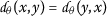
Let \(\mathcal{M}\) be a nonempty set and \(\theta : \mathcal{M}\times \mathcal{M}\rightarrow [1,\infty )\). A function  is called an extended b-metric if for all \(x,y,z\in \mathcal{M}\) it satisfies
- \((d_{\theta }1)\) :
-
 if and only if \(x=y\);
 - \((d_{\theta }2)\) :
-
 ;
; - \((d_{\theta }3)\) :
-
 .
.
 if and only if
  ;
; .
. The pair  is called an extended b-metric space.
It is clear that an extended b-metric space coincides with the corresponding b-metric space, for \(\theta (x,y)=s \geq 1\) where \(s\in \mathbb{R}\) and it turns to be standard metric if \(s=1\).
As expected, the basic topological notions were defined analogously.
Definition 1.2
([5])
Let  be an extended b-metric space.
-
(i)
A sequence \({x_{n}}\) in \(\mathcal{M}\) is said to converge to \(x\in \mathcal{M}\), if for every \(\epsilon >0\) there exists \(N=N(\epsilon )\in \mathbb{N}\) such that
 , for all \(n\geq N\). In this case, we write \(\lim_{n\rightarrow \infty } x_{n} = x\).
 -
(ii)
A sequence \({x_{n}}\) in \(\mathcal{M}\) is said to be Cauchy if for every \(\epsilon >0\) there exists \(N=N(\epsilon )\in \mathbb{N}\) such that
 , for all \(m,n\geq N\).
 , for all
  , for all
 Definition 1.3
([5])
An extended b-metric space  is complete if every Cauchy sequence in \(\mathcal{M}\) is convergent.
Notice that an extended b-metric need not be continuous.
Lemma 1.1
([5])
Let
 be an extended
b-metric space. If
be an extended
b-metric space. If
 is continuous, then every convergent sequence has a unique limit.
For the sake of simplicity, throughout the paper, we assume that  represents a complete extended b-metric space. In addition, we assume that
  is a continuous functional unless otherwise stated.
In what follows, we recollect the main results of Kamran et al. [5] which is an analog of the Banach contraction principle in the context of extended b-metric space.
Theorem 1.3
([5])
Let
\(T:\mathcal{M}\rightarrow \mathcal{M}\)
be mapping. If there exists
 such that

for all
\(x,y\in \mathcal{M} \), where for each
\(x_{0}\in \mathcal{M}\),  , where
\(x_{n}=T^{n}x_{0}\), \(n \in \mathbb{N}\)
Then
T
has precisely one fixed point
u. Moreover, for each
\(y\in \mathcal{M}\), \(T^{n}y\rightarrow u\).
, where
\(x_{n}=T^{n}x_{0}\), \(n \in \mathbb{N}\)
Then
T
has precisely one fixed point
u. Moreover, for each
\(y\in \mathcal{M}\), \(T^{n}y\rightarrow u\).
The main purpose of this paper is to extend the results of Kamran et al. [5] for the well-known fixed point results, including the interesting theorems of Dass and Gupta [3] and Jaggi [4] in the frame of an extended b-metric space.
2 Main results
Theorem 2.1
Let \(T:\mathcal{M}\rightarrow \mathcal{M}\) be a continuous mapping such that, for all distinct \(x,y\in \mathcal{M}\),

where
 and
and

Suppose also that, for each
\(x_{0}\in \mathcal{M}\),  , where
\(x_{n}=T^{n}x_{0}\), \(n\in \mathbb{N}\). Then
T
has a fixed point
u. Moreover, for each
\(x\in \mathcal{M}\), we have
\(T^{n}x \rightarrow u\).
, where
\(x_{n}=T^{n}x_{0}\), \(n\in \mathbb{N}\). Then
T
has a fixed point
u. Moreover, for each
\(x\in \mathcal{M}\), we have
\(T^{n}x \rightarrow u\).
Proof
By presumptions, for given \(x_{0}\in \mathcal{M}\) we construct the sequence \(\{x_{n} \}\) in \(\mathcal{M}\) as \(x_{n}=T^{n}x _{0}=Tx_{n-1}\), for \(n\in \mathbb{N}\). If \(x_{n_{0}}=x_{n_{0}+1}=T x _{n_{0}}\) for some \(n_{0}\in \mathbb{N}_{0}:=\mathbb{N}\cup \{0\}\), then \(x^{\ast }=x_{n_{0}}\) forms a fixed point for T which completes the proof. Consequently, throughout the proof, we assume that
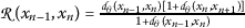
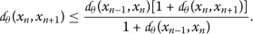
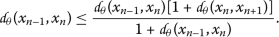
By taking \(x=x_{n-1}\) and \(y=x_{n}\) in the inequality (4), we derive that

with

Thus,

For refining the inequality above, we shall consider the following cases:
-
Case (i).
If
 , then
  , which is a contradiction.
 -
Case (ii).
If
 , then the inequality (4) turns into the inequality below:
 (9)
(9) -
Case (iii).
Suppose that
 ; this yields
 (10)
(10)We shall illustrate that this case is not possible. For this reason, we consider the following subcases:
- Case (iii)a.:
-
Suppose that
 , that is,
 (11)
(11)On the other hand, from (10), we have
 (12)
(12)By a simple calculation, we derive, from the inequality above, that

which contradicts the assumption (11).
- Case (iii)b.:
-
Assume that
 , that is,
 (13)
(13)Furthermore, from (10), we observe that
 (14)
(14)A simple evaluation implies, from the inequality above, that

which contradicts the assumption (13). Hence, Case (iii) does not occur.
 , then
  , which is a contradiction.
 , then the inequality (
 ; this yields

 , that is,


 , that is,


Consequently, we can state that the inequality (9) holds for all these three cases and by applying it recursively we obtain

Since  , we find that

On the other hand, by \((d_{\theta }3)\), together with the triangular inequality, for \(p\geq 1\), we derive that

Notice the inequality above is dominated by  .
.
On the other hand, by employing the ratio test, we conclude that the series  converges to some \(S \in (0,\infty )\). Indeed,
  and hence we get the desired result. Thus, we have

Consequently, we observe, for \(n\leq 1\), \(p\leq 1\), that

Letting \(n\rightarrow \infty \) in (18), we conclude that the constructed sequence \(\{x_{n}\}\) is Cauchy in the extended b-metric space  . Regarding the assumption of the completeness, we conclude that there exists \(u\in \mathcal{M}\) such that \(x_{n}\rightarrow u\) as \(n\rightarrow \infty \). Due to the continuity of T, we shall show that the limit point u is a fixed point of T. Indeed, we have
□
Corollary 2.1
A continuous mapping \(T:\mathcal{M}\rightarrow \mathcal{M}\) has a fixed point provided that, for all distinct \(x,y\in \mathcal{M}\),

where
 , \(i\in \{1,2,3,4 \}\)
with
, \(i\in \{1,2,3,4 \}\)
with
 and for each
\(x_{0}\in \mathcal{M}\),
and for each
\(x_{0}\in \mathcal{M}\),  , where
\(x_{n}=T^{n}x_{0}\), \(n\in \mathbb{N}\).
, where
\(x_{n}=T^{n}x_{0}\), \(n\in \mathbb{N}\).
Proof
The proof follows from Theorem 2.1 by letting  . Indeed, we have

Regarding the analogy, we skip the details. □
Corollary 2.2
Let \(T:\mathcal{M}\rightarrow \mathcal{M}\) be a continuous mapping. Suppose that, for all distinct \(x,y\in \mathcal{M}\), we have the inequality

where \(\alpha , \beta \in [0,1 )\), \(\alpha +\beta <1\). Suppose also that, for each \(x_{0}\in \mathcal{M}\), \(\lim_{n,m\rightarrow \infty } \theta (x_{n}, x_{m})<\frac{1}{\alpha + \beta }\), where \(x_{n}=T^{n}x_{0}\), \(n\in \mathbb{N}\). Then T has a unique fixed point u. Moreover, for each \(x\in \mathcal{M}\), we have \(T^{n}x\rightarrow u\).
Proof
The proof follows from Corollary 2.1 by letting  , where
  and
and  ,
,  . □
. □
Example 2.1
Let  be a complete extended b-metric space, where \(\mathcal{M}= [0,\infty )\) and
  ,
,  and \(\theta : \mathcal{M}\times \mathcal{M}\rightarrow [1,\infty )\) is defined as \(\theta (x,y)=x+y+2\). Let \(T:\mathcal{M}\rightarrow \mathcal{M}\) be defined by \(Tx=\frac{x}{3}\). Obviously,

and, choosing \(\alpha =\frac{2}{9}\) and \(\beta =\frac{1}{9}\), we have
By routine calculation, we obtain

Therefore, all conditions of Corollary 2.2 are satisfied. Thus, T has a fixed point.
Corollary 2.3
Let \(T:\mathcal{M}\rightarrow \mathcal{M}\) be a mapping such that, for all \(x,y\in \mathcal{M}\) we have

where \(\alpha , \beta \in [0,1 )\), \(\alpha +\beta <1\). Suppose also that, for each \(x_{0}\in \mathcal{M}\), \(\lim_{n,m\rightarrow \infty } \theta (x_{n}, x_{m})<\frac{1}{\alpha + \beta }\), where \(x_{n}=T^{n}x_{0}\), \(n\in \mathbb{N}\). Then T has a unique fixed point u. Moreover, for each \(x\in \mathcal{M}\), we have \(T^{n}x\rightarrow u\).
Proof
Letting  , where
  and
and  ,
,  in Corollary 2.1, and following the steps of the proof of Theorem 2.1, we know that there exists \(u\in \mathcal{M}\) such that \(T^{n}x\rightarrow u\). We must prove that this point is the unique fixed point of T. Indeed,

Letting \(n\rightarrow \infty \) in the above inequality we get  . Hence \(Tu=u\).
In order to show the uniqueness, suppose that there exists \(v\in \mathcal{M}\) such that \(Tu=u\neq v=Tv\). Then

which is a contradiction. Thus, we have completed the proof. □
Example 2.2
Let \(\mathcal{M}= \{1,2,3,4,\ldots \}\) and define  as
as

where \(\theta :\mathcal{M}\times \mathcal{M}\rightarrow [1,\infty )\) is a function defined by
Then  forms an extended b-metric space (see Example 3.1 in [10]).
Let \(T:\mathcal{M}\rightarrow \mathcal{M}\) be defined by
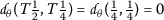
Let also \(\alpha =\frac{1}{16}\) and \(\beta =\frac{1}{8}\). Of course, since  and
and  for any \(x\in \{3,4,5,\ldots \}\), the inequality (22) becomes

For the case \(x=2\) and \(y=1\), we have  and
and  . Obviously, we have

For all other cases,  and the existence of a fixed point is ensured by Corollary 2.3.
Corollary 2.4
Theorem 1.3 is concluded from Corollary 2.2 and hence Theorem 2.1.
Proof
It is sufficient to take \(\alpha =0\). □
2.1 Removing the necessity of the continuity of the functional 

In the following theorem, we relax the condition by removing the continuity of the functional  in the following setting.
Theorem 2.2
Let \(T:\mathcal{M}\rightarrow \mathcal{M}\) be a mapping that satisfies the inequality

for all
\(x,y\in \mathcal{M}\), where
 , be such that, for each
\(x_{0}\in \mathcal{M}\),
, be such that, for each
\(x_{0}\in \mathcal{M}\),  , where
\(x_{n}=T^{n}x_{0}\), \(n\in \mathbb{N}\). Then
T
has a unique fixed point
u. Moreover, for each
\(y\in X\), \(T^{n}y\rightarrow u\).
, where
\(x_{n}=T^{n}x_{0}\), \(n\in \mathbb{N}\). Then
T
has a unique fixed point
u. Moreover, for each
\(y\in X\), \(T^{n}y\rightarrow u\).
Proof
By taking \(x=x_{n-1}\) and \(y=x_{n}\) in the inequality (24), we get

Recursively, we derive that

and regarding that  , we derive that

On the other hand, by following the same lines in the previous theorem, we conclude that \(\{x_{n}\}\) is a Cauchy sequence. Since \(\mathcal{M}\) is complete, there exists \(u\in \mathcal{M}\) such that the sequence \(\{x_{n}=T^{n}x_{0}\}\) converges to u, that is,

As a next step, we shall prove that u is a fixed point of T. By using (24) and the triangle inequality, we have

Letting \(n\rightarrow \infty \), and taking (27) and (28) into account, we get

Accordingly, we have  , that is, \(Tu=u\).
Lastly, we shall indicate that this fixed point is unique. Suppose, on the contrary, that it is not unique. Thus, there exists another fixed point v of T that is distinct from u. Now, by using (24) and  ,
,

which shows that \(u=v\). Therefore, T has a unique fixed point. □
Example 2.3
Let \(\mathcal{M}= \{\frac{1}{2}, \frac{1}{4}, \frac{1}{8} \}\) and the functions \(\theta :\mathcal{M}\times \mathcal{M}\rightarrow [1, \infty )\),  be defined as \(\theta (x,y)=x+y+1\) and

Let  and \(T:\mathcal{M}\rightarrow \mathcal{M}\) be defined by
We have \(T^{n}x\rightarrow 0\) for any \(x\in \mathcal{M}\) and  .
.
But
and

which proves that  is an extended b-metric on \(\mathcal{M}\).
We will consider the following cases:
-
(i)
For \(x=\frac{1}{2}\), \(y=\frac{1}{4}\), we have
 , so the condition from Theorem 2.2 is satisfied.
 -
(ii)
For \(x=\frac{1}{2}\), \(y=\frac{1}{8}\)
-
(iii)
For \(x=\frac{1}{4}\), \(y=\frac{1}{8}\)

 , so the condition from Theorem

Therefore all conditions of Theorem 2.2 are satisfied. Hence T has a unique fixed point, \(x=\frac{1}{4}\).
Corollary 2.5
Let \(T:\mathcal{M}\rightarrow \mathcal{M}\) be a mapping that satisfies

for all \(x,y\in \mathcal{M}\), where \(\alpha , \beta \in [0,1 )\), \(\alpha +\beta <1\) are such that, for each \(x_{0}\in \mathcal{M}\), \(\lim_{n,m\rightarrow \infty } \theta (x_{n}, x_{m})<\frac{1}{\alpha + \beta }\), where \(x_{n}=T^{n}x_{0}\), \(n\in \mathbb{N}\). Then T has a unique fixed point u. Moreover, for each \(x\in \mathcal{M}\), \(T^{n}x\rightarrow u\).
3 Conclusion
It is clear that the corresponding results in the setting of both b-metric space and standard metric space can be included in our results, by letting \(\theta (x,y)=s\geq 1\) and \(\theta (x,y)= 1\), respectively, in the related places. In particular, the main results of Dass and Gupta [3], Jaggi [4] and also the well-known Banach contraction mapping principle are derived from our results.
Change history
29 August 2019
The authors would like to express their sincere appreciation to the Deanship of Scientific Research at King Saud University for funding this group No. RG-1437-017. The corrected funding of the original article [1] is listed below.
References
Arshad, M., Karapınar, E., Jamshaid, A.: Some unique fixed point theorems for rational contractions in partially ordered metric spaces. J. Inequal. Appl. 2013, Article ID 248 (2013)
Chandok, S., Karapinar, E.: Common fixed point of generalized rational type contraction mappings in partially ordered metric spaces. Thai J. Math. 11(2), 251–260 (2013)
Dass, B.K., Gupta, S.: An extension of Banach contraction principle through rational expressions. Indian J. Pure Appl. Math. 6, 1455–1458 (1975)
Jaggi, D.S.: Some unique fixed point theorems. Indian J. Pure Appl. Math. 8, 223–230 (1977)
Kamran, T., Samreen, M., Ain, O.U.: A generalization of b-metric space and some fixed point theorems. Mathematics 5, 19 (2017)
Karapinar, E., Marudai, M., Pragadeeswarar, V.: Fixed point theorems for generalized weak contractions satisfying rational expression on a ordered partial metric space. Lobachevskii J. Math. 34(1), 116–123 (2013)
Karapinar, E., Roldan, A., Sadarangani, K.: Existence and uniqueness of best proximity points under rational contractivity conditions. Math. Slovaca 66(6), 1427–1442 (2016)
Karapinar, E., Shatanawi, W., Tas, K.: Fixed point theorem on partial metric spaces involving rational expressions. Miskolc Math. Notes 14(1), 135–142 (2013)
Mustafa, Z., Karapınar, E., Aydi, H.: A discussion on generalized almost contractions via rational expressions in partially ordered metric spaces. J. Inequal. Appl. 2014, 219 (2014)
Samreen, M., Kamran, T., Postolache, M.: Extended b-metric space, extended b-comparison function and nonlinear contractions. Sci. Bull. “Politeh.” Univ. Buchar., Ser. A, Appl. Math. Phys. 80(4), 21–28 (2018)
Funding
Not applicable.
Author information
Authors and Affiliations
Contributions
All authors contributed equally and significantly in writing this article. All authors read and approved the final manuscript.
Corresponding author
Ethics declarations
Competing interests
The authors declare that they have no competing interests.
Additional information
Publisher’s Note
Springer Nature remains neutral with regard to jurisdictional claims in published maps and institutional affiliations.
Rights and permissions
Open Access This article is distributed under the terms of the Creative Commons Attribution 4.0 International License (http://creativecommons.org/licenses/by/4.0/), which permits unrestricted use, distribution, and reproduction in any medium, provided you give appropriate credit to the original author(s) and the source, provide a link to the Creative Commons license, and indicate if changes were made.
About this article

Cite this article
Alqahtani, B., Fulga, A., Karapınar, E. et al. Contractions with rational inequalities in the extended b-metric space. J Inequal Appl 2019, 220 (2019). https://doi.org/10.1186/s13660-019-2176-6
Received:
Accepted:
Published:
DOI: https://doi.org/10.1186/s13660-019-2176-6