Abstract
Background
Using visual, biological, and electronic health records data as the sole input source, pretrained convolutional neural networks and conventional machine learning methods have been heavily employed for the identification of various malignancies. Initially, a series of preprocessing steps and image segmentation steps are performed to extract region of interest features from noisy features. Then, the extracted features are applied to several machine learning and deep learning methods for the detection of cancer.
Methods
In this work, a review of all the methods that have been applied to develop machine learning algorithms that detect cancer is provided. With more than 100 types of cancer, this study only examines research on the four most common and prevalent cancers worldwide: lung, breast, prostate, and colorectal cancer. Next, by using state-of-the-art sentence transformers namely: SBERT (2019) and the unsupervised SimCSE (2021), this study proposes a new methodology for detecting cancer. This method requires raw DNA sequences of matched tumor/normal pair as the only input. The learnt DNA representations retrieved from SBERT and SimCSE will then be sent to machine learning algorithms (XGBoost, Random Forest, LightGBM, and CNNs) for classification. As far as we are aware, SBERT and SimCSE transformers have not been applied to represent DNA sequences in cancer detection settings.
Results
The XGBoost model, which had the highest overall accuracy of 73 ± 0.13 % using SBERT embeddings and 75 ± 0.12 % using SimCSE embeddings, was the best performing classifier. In light of these findings, it can be concluded that incorporating sentence representations from SimCSE’s sentence transformer only marginally improved the performance of machine learning models.
Introduction
Cancer is a disease where some cells in the body grow destructively and may spread to other body organs [1]. Typically, cells grow and expand through a cell division process to create new cells that can be used to repair old and damaged ones. However, this phenomenon can be interrupted resulting in abnormal cells growing uncontrollably to form tumors that can be malignant (harmful) or benign (harmless) [2,3,4].
With the introduction of genomic data that allows physicians and healthcare decision-makers to learn more about their patients and their response to the therapy they provide to them, this has facilitated the use of machine learning and deep learning to solve challenging cancer problems. These kinds of problems involve various tasks such as designing cancer risk-prediction models that try to identify patients that are at a higher risk of developing cancer than the general population, studying the progression of the disease to improve survival rates, and building methods that trace the effectiveness of treatment to improve treatment options [5,6,7].
Generally, the first step in analyzing genomic data to address cancer-related problems is selecting a data representation algorithm that will be used to estimate contiguous representations of the data. Examples of such algorithms include Word2vec [8], GloVe [9], and fastText [10]. The more recent and advanced versions of these algorithms are sentence transformers which are used to compute dense vector representations for sentences, paragraphs, and images. Similar texts are found close together in a vector space and dissimilar texts are far apart [11]. In this work, two such sentence transformers (SBERT and SimCSE) are proposed for detecting cancer in tumor/normal pairs of colorectal cancer patients. In this new approach, the classification algorithm relies on raw DNA sequences as the only input source. Moreover, this work provides a review of the most recent developments in cancers of the human body using machine learning and deep learning methods. While these kinds of similar reviews already exist in the literature, this study solely focuses on work that investigates four cancer types that have high prevalence rates worldwide [12] (lung, breast, prostate, and colorectal cancer) that have been published in the last five years (2018–2022).
Detection of cancer using machine learning
Lung cancer
Lung cancer is the type of cancer that begins in the lungs and may spread to other organs in the body. This kind of cancer occurs when malignant cells develop in the tissue of the lung. There are two types of lung cancer: non-small-cell lung cancer (NSCLC) and small-cell lung cancer (SCLC). These cancers develop differently and thus their treatment therapies are different. Smoking (tobacco) is the leading cause of lung cancer. However, non-smokers can also develop lung cancer [13, 14].
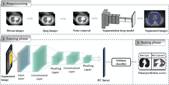
When it comes to the detection of lung cancer using machine learning (Fig. 1), a considerable amount of work has been done, a summary is provided (Table 1). Typically, a series of pre-processing steps using statistical methods and pretrained CNNs for feature extraction are carried out from several input sources (mostly images) to delineate the cancer region. Then, the extracted features are fed as input to several machine learning algorithms for classification of various lung cancer tasks such as the detection of malignant lung nodules from benign ones [15,16,17], the separation of a set of normalized biological data points into cancerous and non cancerous groups [18], and a basic comparative analysis of powerful machine learning algorithms for lung cancer detection [19].
Generalized machine learning framework for lung cancer prediction [33]
The lowest classification accuracy reported in Table 1 was 74.4% by work in [20]. In this work, a pretrained CNN model (DenseNet) was used to develop a lung cancer detection model. First, the model was fine-tuned to identify lung nodules from chest X-rays using the ChestX-ray14 dataset [21]. Second, the model was fine-tuned to identify lung cancer from images in the JSRT (Japanese Society of Radiological Technology) dataset [22].
The highest classification accuracy of 99.7% for lung cancer classification was reported by work in [18]. This study developed the Discrete AdaBoost Optimized Ensemble Learning Generalized Neural Network (DAELGNN) framework that uses a set of normalized biological data points to create a neural network that separates normal lung features from non-normal (cancerous) features.
Popular datasets used in lung cancer research using machine learning include the Lung Image Database Consortium (LIDC) and Image Database Resource Initiative (IDRI) (LIDC-IDRI) database [23] initiated by the National Cancer Institute (NCI), and the histopathological images of lung and colon cancer (LC2500) database [24].
Breast cancer
Breast Cancer is a malignant tumor or growth that develops in the cells of the breast [34]. Similar to lung cancer, breast cancer also has the ability to metastasize to near by lymph nodes or to other body organs. Towards the end of 2020, there were approximately 7.8 million women who have been diagnosed with breast cancer, making this type of cancer the most prevalent cancer in the world. Risk factors of breast cancer include age, obesity, abuse of alcohol, and family history [35,36,37].
Currently, there is no identified prevention procedure for breast cancer. However, maintaining a healthy living habit such as physical exercise and less alcohol intake can reduce the risk of developing breast cancer [38]. It has also been said that early detection methods that rely on machine learning can improve the prognosis. As such, this type of cancer has been extensively studied using machine learning and deep learning [39, 40].
As with lung cancer (Sect. 2.1), a great deal of work has been executed in developing breast cancer detection models, a generalized approach that illustrates the process using machine learning is provided (Fig. 2).
Generalized machine learning framework for breast cancer prediction [45]
Several classification problems have been studied that mainly focuses on the detection of breast cancer from thermogram images [41], handrafted features [42], mammograms [43], and whole slide images [44]. To develop a breast cancer detection model, initially, a pre-processing step is implemented that aims to extract features of interest. Then, the extracted features are provided as input to machine learning models for classification. This framework is implemented by several works such as [45,46,47,48].
One of the most popular datasets used for breast cancer detection using machine learning is the Wisconsin breast cancer dataset [42]. This dataset consists of features that describe the characteristics of the cell nuclei that is present in the image such as the diagnosis features (malignant or benign), radius, symmetry, and texture. Studies that used this dataset are [49, 50]. In [49], the authors scaled the Wisconsin breast cancer features to be in the range between 0 and 1, then used a CNN for classification into benign or malignant. As opposed to using a CNN for classification, the authors [50] used traditional machine learning classifiers (Linear Regression, Multilayer Perceptron (MLP), Nearest Neighbor search, Softmax Regression, Gated recurrent Unit (GRU)-SVM, and SVM). For data pre-processing, the study used the Standard Scaler technique that standardizes data points by removing the mean and scaling the data to unit variance. The MLP model outperformed the other models by producing the highest accuracy of 99.04% which is almost similar to the accuracy of 99.6% that was reported by [49].
Different form binary classification of benign or malignant classes, a study [46] proposed a two-step approach to design a breast cancer multi-class classification model that predicts eight categories of breast cancer. In the first approach, the study used handcrafted features that are generated from histopathology images. These features were then fed as input to classical machine learning algorithms (RF, SVM, Linear Discriminant Analysis (LDA)). In the second approach, the study applied a transfer learning method to develop the multi-classification deep learning framework where pretained CNNs (ResNet50, VGG16 and VGG19) were used as feature extractors and baseline models. It was then found that the VGG16 pretrained CNN with the linear SVM provided the best accuracy in the range of 91.23%\(-\)93.97%. This study also found that using pretrained CNNs as feature extractors improved the classification performance of the models.
The Table 2 provides a summary of the work that has been done to detect breast cancer using machine learning.
Prostate cancer
Prostate cancer is a type of cancer that develops when cells in the prostate gland start to grow uncontrollably (malignant). Prostate cancer often presents with no symptoms and grows at a slow rate. As a result, some men may die of other diseases before the cancer starts to cause notable problems. Comparably, prostate cancer can also be aggressive and metastasize to other body organs that are outside the confines of the prostate gland. Risk factors that are associated with this type of cancer include age, specifically, men that are above the age of 50. Other risk factors include ethnicity, family history of prostate cancer, breast or ovarian cancer, and obesity [61,62,63].
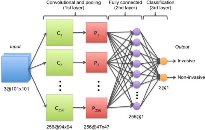
Transfer learning, which is defined as the reuse of a pretrained model on a new problem, was frequently applied to develop prostate cancer detection models using machine learning (Fig. 3). For example, a study [64] applied a transfer learning approach to detect prostate cancer on magnetic resonance images (MRI) by using a pretrained GoogleNet. A series of features such as texture, entropy, morphological, scale invariant feature transform (SIFT), and Elliptic Fourier Descriptors (EFDs) were extracted from the images as described by [65, 66]. Other traditional machine learning classifiers were also evaluated such as Decision trees, and SVM Gaussian however, the GoogleNet model outperformed the other models.
Generalized machine learning framework for prostate cancer prediction using 3-d CNNs, pooling layers, and a fully connected layer for classification [69]
Also using transfer learning, a study [67] developed a prostate cancer detection model by using MRI images and ultrasound (US) images. The model was developed in two stages: first, pretrained CNNs were used for classification of the US and MRI images into benign or malignant. While the pretrained CNNs performed well on the US images (accuracy 97%), the performance on the MRI images was not adequate. As a result, the best-performing pretrained CNN(VGG16) was selected and used as a feature extractor. The extracted features were then provided as input to traditional machine learning classifiers.
Another study [68] also used the same dataset as in [64] to create a prostate cancer detection model. However, instead of using GoogleNet as seen previously by [64], this study used a ResNet-101 and an autoencoder for feature reduction. Other machine learning models were also evaluated but, the study concluded that the pretrained ResNet-101 outperformed the other models with an accuracy of 100%. These results are similar to a previous study [64] that showed how pretrained CNNs outperform traditional machine learning models for cancer detection.
Table 3, gives a summary of recent work that has been executed to create prostate cancer detection models.
Colorectal cancer
Colorectal cancer is a type of cancer that starts in the colon or rectum. The colon and rectum are parts of the human body that make up the large intestine that is part of the digestive system. A large part of the large intestine is made up of the colon which is divided into a few parts namely: ascending colon, transverse colon, descending colon, and sigmoid colon. The main function of the colon is to absorb water and salt from the remaining food waste after it has passed through the small intestine. Then, the waste that is left after passing through the colon goes into the rectum and is stored there until it is passed through the anus. Some colorectal cancers called polyps first develop as growth that can be found in the inner lining of the colon or rectum. Overtime, these polyps can develop into cancer, however, not all of them can be cancerous. Some of the risk factors of colorectal cancer include obesity, lack of exercise, diets that are rich in red meat, smoking, and alcohol [82,83,84].
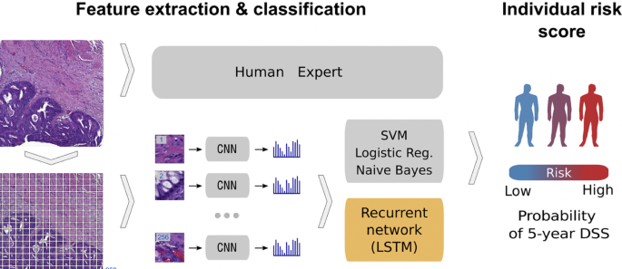
In relation to the advancements made in colorectal cancer research using machine learning (Fig. 4), various tasks have been investigated such as predicting high-risk colorectal cancer from images, predicting five-year disease-specific survival, colorectal cancer tissue multi-class classification, and identifying the risk factors for lymph node metastasis (LNM) in colorectal cancer patients [85,86,87,88]. As with prostate cancer, transfer learning was mostly applied to extract features from various input sources such as colonoscopic images, tissue microarrays (TMA), and H &E slide images. Then, the extracted features were fed as input to machine learning algorithms for classification.
Using a deep CNN network to predict colorectal cancer outcome using images [86]
One common observation with regards to colorectal cancer models, is that the predictions made from the models were compared to those of experts. For example, a study [85] developed a deep learning model that detects high risk colorectal cancer from whole slide images that were collected from colon biopsies. The deep learning model was created in two stages: first, a segmentation procedure was executed to extract high risk regions from whole slide images. This segmentation procedure applied Faster-Region Based Convolutional Neural Network (Faster-RCNN) that uses a ResNet-101 model as a backbone for feature extraction. The second stage of implementing the model applied a gradient-boosted decision tree on the output of the Faster-RCNN deep learning model to classify the slides into either high or low risk colorectal cancer, and achieved an AUC of 91.7%. The study then found that the predictions made from the validation set were in agreement with annotations made by expert pathologists.
Work in [89] also compared predictions made by the Microsatellite instability (MSI)-predictor model with those of expert pathologists and found that experts achieved a mean AUROC of 61% while the model achieved an AUROC of 93% on a hold-out set and 87% on a reader experiment.
A previous study [90] developed a model named CRCNet, based a pretrained dense CNN, that automatically detects colorecal cancer from colonoscopic images and found that the model exceeded the avarage performance of expert endoscopists on a recall rate of 91.3% versus 83.8%.
In Table 4, a summary is provided that describes the work that has been executed in colorectal cancer research using machine learning.
In summary of the literature survey (Sect. 2), a series of machine learning approaches for the detection of cancer were analysed. Imaging datasets, biological and clinical data, and EHRs were primarily employed as the initial input source when developing cancer detection algorithms. This procedure involved a few preprocessing steps. First, the input source was typically preprocessed at the beginning stages of the experiment to extract regions or features of interest. Next, the retrieved set of features were then applied to downstream machine learning classifiers for cancer prediction. In this work, as opposed to using imaging datasets, clinical and biological data or, EHRs as the starting input source, this work proposes to use raw DNA sequences as the only input source. Moreover, contrary to using statistical methods or advanced CNNs for data extraction and representation, this work proposes to use state-of-the-art sentence transformers namely: SBERT and SimCSE. As far as we are aware, these two sentence transformer models have not been applied for learning representations in cancer research. The learned representations will then be fed as input to machine learning algorithms for cancer prediction.
Methods
Data description
In this study, 95 samples from colorectal cancer patients and matched-normal samples from previous work [104] were analysed. Exon sequences from two key genes: APC and ATM were used. The full details of the exons that were used in this study is shown Tables 5 and 6. Table 7 shows the data distribution among the normal/tumor DNA sequences. Ethics approval was granted by the University of Pretoria EBIT Research Ethics Committee (EBIT/139/2020).
Data encoding
To encode the DNA sequences, state-of-the-art sentence transformers: Sentence-BERT [105] and SimCSE [105] were used. These transformers are explained in the next subsection.
Sentence-BERT
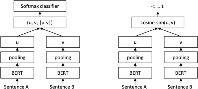
Sentence-BERT (SBERT) (Fig. 5) adapts the pretrained BERT [106] and RoBERTa [107] transformer network and modifies it to use a siamese and triplet network architectures to compute fixed-sized vectors for more than 100 languages. The sentence embeddings can then be contrasted using the cosine-similarity. SBERT was trained on the combination of SNLI data [108] and the Multi-Genre NLI dataset [109].
SBERT architecture with classification objective function (left) and the regression objective function (right) [105]
In its architecture, SBERT adds a default mean-pooling procedure on the output of the BERT or RoBERTa network to compute sentence embeddings. SBERT implements the following objective functions: classification objective function, regression objective function, and the triplet objective function. In the classification objective function, the sentence embeddings of two sentence pairs u and v are concatenated using the element-wise difference \(\mid u-v \mid\) and multiplied with the trainable weight \(W_{t} \epsilon {\mathbb {R}}^{3n *k}\):
where n is the length or dimension of the sentence embeddings and k is the value of the target labels.
The regression objective function makes use of mean-squared-error loss as the objective function to compute the cosine-similarity between two sentence embeddings u and v.
The triplet objective function fine-tunes the network such that the distance between an anchor sentence a and a positive sentence p is smaller than the distance between sentence a and the negative sentence n.
Using the pretrained SBERT model: all-MiniLM-L6-v2, each DNA sequence was represented by a 384-dimensional vector.
SimCSE
As with SBERT, Simple Contrastive Sentence Embedding (SimCSE) [110] (Fig. 6 is a transformer based model that modifies the BERT/RoberTa encoder to generate sentence embeddings. It uses a contrastive learning approach that aims to learn sentence representations by pulling close neighbours together and propelling non-neighbours. SimCSE comes in two learning forms: unsupervised and supervised SimCSE. In unsupervised SimCSE, the network is fine-tuned to predict the input sentence itself using dropout as noise then, the other sentences that are in the mini-batch are taken as negatives. In this case, dropout acts as a data augmentation method while previous [111, 112] methods have used word deletion, reordering, and substitution as a way of generating positive instances. In unsupervised SimCSE, an input sentence is fed twice to the encoder then, two embeddings with different dropout masks z, \(z'\) are generated as output. The training objective for SimCSE is:
where z is the standard dropout mask that are found in Transformers and no additional dropout mask is added [110].
Unsupervised SimCSE (a) and supervised SimCSE (b) [110]
In supervised SimCSE, positive pairs are taken from the natural language inference (NLI) datasets and used to optimise the following equation:
where \(\tau\) is a temperature hyperparamter and \(sim(h_{1},h_{2})\) is the cosine similarity.
Using the unsupervised pretrained SimCSE model: unsup-simcse-bert-base-uncased, each DNA sequence was represented by a 768-dimensional vector.
K-means clustering
The k-means clustering algorithm was used to visualize the sentence representations generated from SBERT and SimCSE in an unsupervised approach. The k-means algorithm divides the data points into k clusters where each data point is said to belong to the cluster centroid closest to it. Since the data consists of two types of documents (tumor vs. normal), the k-means algorithm was asked to find 2 clusters n and assign each DNA sequence to its closest centroid [113].
Machine learning experiments
A total of three machine learning algorithms were used for classification: Light Gradient Boosting (LightGBM), eXtreme Gradient Boosting (XGBoost), and Random Forest (RF).
eXtreme gradient boosting (XGBoost)
eXtreme Gradient Boosting (XGBoost), is an efficient implementation of the gradient boosting algorithm. Gradient boosting belongs to a group of ensemble machine learning algorithms that be used to solve classification or regression problems. The ensembles are created from decision trees that are added one at a time to the ensemble, and fit to correct the classification error that were made by prior trees [114].
Light gradient boosting (LightGBM)
Light Gradient Boosting (LightGBM) machine is also a gradient boosting model that is used for ranking, classification, and regression. In contrast to XGBoost, LightGBM splits the tree vertically as opposed to horizontally. This method of growing the tree leaf vertically results in more loss reduction and provides higher accuracy while also being faster. LightGBM uses the Gradient-based One-Side Sampling (GOSS) method to filter out data instances for obtaining the best split value while XGBoost uses a pre-sorted and Histogram-based algorithm for calculating the best split value [115].
Random forest (RF)
Random forest (RF) is a supervised machine learning that is used in classification and regression tasks. It creates decision tress based on different samples and takes the majority vote for classification or average for regression. While XGBoost and LightGBM use a gradient boosting method, Random Forest uses a bagging method. The bagging method builds a different training subset from the training data with replacement. Each model is trained separately and the final result is based on a majority voting after consolidating the results of all the models [116].
Convolutional neural network (CNN)
Convolutional neural networks (CNNs) are a subset of neural networks that are frequently used to process speech, audio, and visual input signals. Convolutional, pooling, and fully connected (FC) layers are the three types of layers that are generally present in CNNs. The convolutional layer is the fundamental component of a CNN and is in charge of performing convolutional operations on the input before passing the outcome to the following layer. Then, the input is subjected to dimensionality reduction using pooling layers that reduces the number of parameters in the input. The FC layer uses a variety of activation functions, including the softmax activation function and the sigmoid activation function, to carry out the classification task using the features retrieved from the network’s prior layers [117, 118]. In this work, a three-layer CNN model with a sigmoid activation function will be supplied with the embedding features that were retrieved by SBERT and SimCSE sentence transformers. Due to computational limitations, the network will be trained over 10 epochs using the RMSprop optimizer and cross-validated over five folds.
Performance evaluation metrics
To measure the performance of the machine learning models, the average performance of the models were reported using 5-fold cross validation and the following metrics were used: accuracy, precision, recall and F1 score. In Table 8, the definition of these metrics is provided.
This section described the datasets used in the study as well as data representation methods and machine learning algorithms that were applied in this work. In the next section, the results of the applied methods are described.
Results
Visualizations
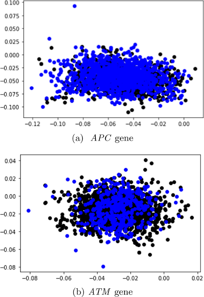
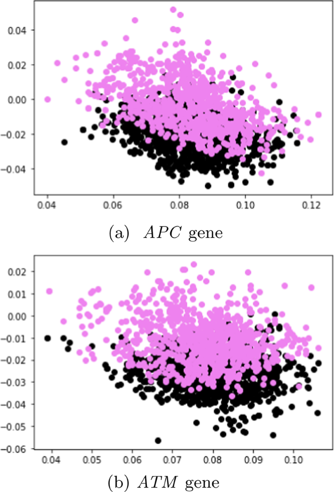
In this subsection, unlabeled data from SBERT and SimCSE representations were explored and visualized with the k-means clustering algorithm. The representations of the SBERT algorithm (Fig. 7) revealed more overlap between the data points in comparison to the representations of the SimCSE algorithm (Fig. 8). In the next subsection, machine learning models are evaluated to reveal if there is sufficient signal in the representations of the two sentence transformers that can discriminate between tumor and normal DNA sequences.
Comparative performance of the machine learning results
SBERT before SMOTE
Table 9 presents the performance of the machine learning models on the dev set in terms of the average accuracy, averaged over the five folds using the SBERT representations. More performance metrics such as F1 score, recall, and precision are reported in the Additional file 1 (Appendix A).
APC
Considering that the tumor DNA sequences belonging to the APC gene comprised of \(\approx\) 64% of the data before SMOTE sampling, the machine learning models classified most sequences as positive (tumor); with the CNN achieving the best overall with the highest accuracy of 67.3 ± 0.04%.
ATM
In contrast to the data distribution of the APC gene before SMOTE sampling, the original data distribution of sequences from the ATM gene were relatively balanced as the tumor sequences comprised of 53% of the total data, and normal DNA sequences made up 47%. Moreover, as opposed to predicting nearly all sequences as positive, the machine learning models demonstrated an unbiased above-average performance as the highest performing model (XGBoost) achieved an accuracy of 73. ± 0.13 %.
SBERT after SMOTE
APC
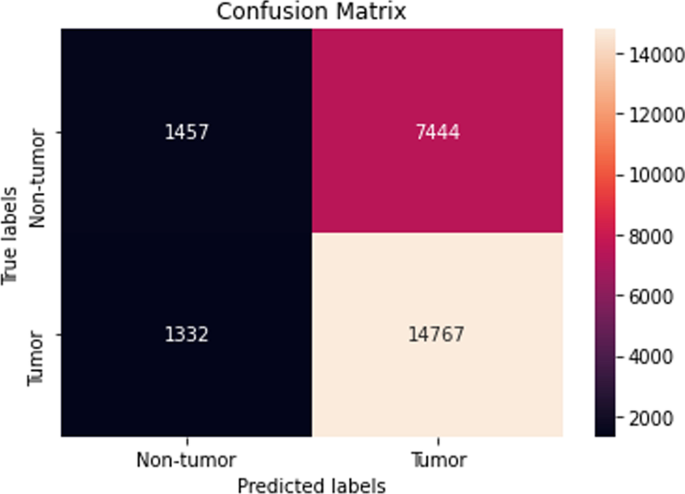
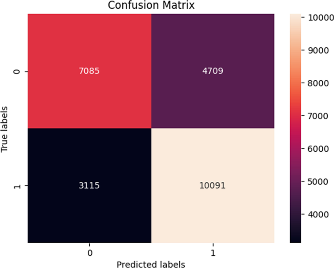
The performance of the majority of the machine learning classifiers after applying SMOTE remained consistent in that very little improvement or decline was observed. Moreover, while the CNN model previously obtained the highest overall accuracy before SMOTE oversampling, it performed the worst after applying SMOTE with a reported accuracy of 47. ± 17.4 %. Although biased, the LightGBM classifier reached the highest accuracy of 64.9 ± 0.29 %. Its confusion matrix is shown (Fig. 9).
ATM
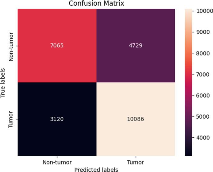
The same trend as seen in the previous Sect. 4.2.2 was also observed in this section with sequences from the ATM gene. Here, the performance of the machine learning models after SMOTE sampling was relatively similar to the performance of the machine learning models before SMOTE sampling as the XGBoost still maintained the best overall accuracy of 73. ± 0.13 % (Fig. 10).
SimCSE before SMOTE
Table 9 also presents the performance of the machine learning models in terms of the average accuracy, averaged over the five folds using the SimCSE representations. Supplementary performance metrics are reported (Additional file 1: Appendix A).
APC
In this experimental setting, the performance of the machine learning models with SBERT representations before SMOTE sampling was similar to the performance of the models with SimCSE representations before SMOTE sampling. Here, the CNN achieved the best accuracy of 67. ± 0.0 %.
ATM
A similar pattern as in the previous Sect. (APC, SimCSE before SMOTE) was also detected in this setting when using sequences from the ATM gene in that the performance of the SimCSE models were almost similar to the performance of the SBERT models (before SMOTE) with slight improvement. The LightGBM model achieved the highest accuracy of 74. ± 0.18 % which was an improvement in accuracy of approximately 4 %.
SimCSE after SMOTE
APC
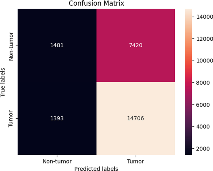
The LightGBM model achieved the highest accuracy of 64.7 ± 0.29 (Fig. 11), which was indistinguishable to the performance reported before SMOTE oversampling.
ATM In this final experimental setting, the results demonstrated a consistent performance before SMOTE sampling and after SMOTE sampling. The highest performing model was the Random forest model as it achieved an average accuracy of 71.6 ± 1.47 % (Fig. 12).
In Table 10, the experiments were repeated on an additional unseen test set. Overall, the machine learning models demonstrated a slight increase in the accuracy as the highest performing model, XGBoost, achieved an average accuracy of 75. ± 0.12 % using SimCSE representations from the ATM gene.
Discussion
This paper provided a literature review of how cancer has been detected using various machine learning methods. Additionally, this work developed machine learning models that detect cancer using raw DNA sequences as the only input source. The DNA sequences were retrieved from matched tumor/normal pairs of colorectal cancer patients as described by previous work [104]. For data representation, two state-of-the-art sentence transformers were proposed: SBERT and SimCSE. To the best of our knowledge, these two methods have not been used to represent DNA sequences in cancer detection problems using machine learning. In summary of the results, we note that using SimCSE representations only marginally improved the performance of the machine learning models.
The ability to detect cancer by relying on human DNA as the only input source to a learning algorithm was one of the significant contributions of this work. We acknowledge that similar research investigating the role that the DNA plays in various cancer types has been conducted in the past. In contrary, the way the DNA was represented for the learning algorithms in our work is different from that in earlier research. An example would be work performed by [120] that used cell-free DNA (cfDNA) data from shallow whole-genome sequencing to uncover patterns associated with a number of different cancers including Hodgkin lymphoma, diffuse large B-cell lymphoma, and multiple myeloma. This study used PCA transformed genome-wide coverage features and applied them as input to a support vector algorithm to predict cancer status rather than employing sentence transforms for data representation as was done in our study. Another study [121] also used cfDNA sequences to predict cancer tissue sequences from healthy ones. In this work, reads from hepatocellular carcinoma (HCC) patients and healthy individuals were integrated with methylation information and then, a deep learning model was created to predict the reads that originated from a cancer tissue. The deep learning model consisted of a 1-d CNN followed by a maxpooling layer, a bi-directional LSTM, a 1-d CNN, and three dense layers. To represent the cfDNA sequences and methylation information, the variables were encoded into a one-hot encoded matrix that was then provided as input to the deep learning model for classification. Different from relying on raw DNA or cfDNA data to develop cancer detection frameworks, a study [122] consolidated methods from variant calling and machine learning to develop a model that detects cancers of unknown primary (CUP) origin which account for approximately 3% of all cancer diagnoses. This work employed whole-genome-sequencing-based mutation features derived from structural variants that were generated through variant calling and fed them as input to an ensemble of random forest binary classifiers for the detection of 35 different cancers.
Limitations of the study
The machine learning experiments were only performed on two key genes: APC and APC, therefore it would have been interesting to see how the models generalize across various genes. The common disadvantage of conducting the experiments on multiple genes or whole genome sequencing data is that they require more computational resources which have a direct impact on cost. Another limitation of this work is that only two pretrained models were used for generating the sentence representations. Since there are several other pretrained models that are publicly available to choose from, some pretrained models were slower to execute than others hence a decision was made to focus on pretrained models that provided fast execution.
Conclusion
This article reviewed the literature and demonstrated how various machine learning techniques have been used to identify cancer. Given that they are the most common malignancies worldwide, this work placed a special emphasis on four cancer types: lung, breast, prostate, and colorectal cancer. Then, a new method for the identification of colorectal cancer employing SBERT and SimCSE sentence representations was presented. Raw DNA sequences from matched tumor/normal pairs of colorectal cancer served as the sole input for this approach. The learned representations were then provided as input to machine learning classifiers for classification. In light of the performance of the machine learning classifiers, XGBoost was found to be the best performing classifier overall. Moreover, using SimCSE representations only marginally improved the classification performance of the machine learning models.
Availability of data and materials
The data can be accessed at the host database (The European Genome-phenome Archive at the European Bioinformatics Institute, accession number: EGAD00001004582 Data access).
References
Jones PA, Baylin SB. The epigenomics of cancer. Cell. 2007;128(4):683–92.
What Is Cancer? National Cancer Institute. https://www.cancer.gov/about-cancer/understanding/what-is-cancer
Zheng R, Sun K, Zhang S, Zeng H, Zou X, Chen R, Gu X, Wei W, He J. Report of cancer epidemiology in china, 2015. Zhonghua zhong liu za zhi. 2019;41(1):19–28.
Hegde PS, Chen DS. Top 10 challenges in cancer immunotherapy. Immunity. 2020;52(1):17–35.
Kourou K, Exarchos TP, Exarchos KP, Karamouzis MV, Fotiadis DI. Machine learning applications in cancer prognosis and prediction. Comput Struct Biotechnol J. 2015;13:8–17.
Iqbal MJ, Javed Z, Sadia H, Qureshi IA, Irshad A, Ahmed R, Malik K, Raza S, Abbas A, Pezzani R, et al. Clinical applications of artificial intelligence and machine learning in cancer diagnosis: looking into the future. Cancer Cell Int. 2021;21(1):1–11.
Loud JT, Murphy J. Cancer screening and early detection in the 21st century. Semin Oncol Nurs. 2017;33:121–8.
Goldberg Y, Levy O. word2vec explained: deriving mikolov et al.’s negative-sampling word-embedding method. 2014; arXiv preprint arXiv:1402.3722
Pennington J, Socher R, Manning CD. Glove: global vectors for word representation. In: Proceedings of the 2014 conference on empirical methods in natural language processing (EMNLP). 2014. p. 1532–43.
Bojanowski P, Grave E, Joulin A, Mikolov T. Enriching word vectors with subword information. Trans Assoc Comput Linguist. 2017;5:135–46.
Church KW. Word2vec. Natl Lang Eng. 2017;23(1):155–62.
Cancer. World Health Organization. https://www.who.int/news-room/fact-sheets/detail/cancer
Bade BC, Cruz CSD. Lung cancer 2020: epidemiology, etiology, and prevention. Clin Chest Med. 2020;41(1):1–24.
Barta JA, Powell CA, Wisnivesky JP. Global epidemiology of lung cancer. Ann Global Health. 2019;85:1.
de Carvalho Filho AO, Silva AC, de Paiva AC, Nunes RA, Gattass M. Classification of patterns of benignity and malignancy based on ct using topology-based phylogenetic diversity index and convolutional neural network. Pattern Recogn. 2018;81:200–12.
Rodrigues MB, Da Nobrega RVM, Alves SSA, Reboucas Filho PP, Duarte JBF, Sangaiah AK, De Albuquerque VHC. Health of things algorithms for malignancy level classification of lung nodules. IEEE Access. 2018;6:18592–601.
Asuntha A, Srinivasan A. Deep learning for lung cancer detection and classification. Multim Tools Appl. 2020;79(11):7731–62.
Shakeel PM, Tolba A, Al-Makhadmeh Z, Jaber MM. Automatic detection of lung cancer from biomedical data set using discrete adaboost optimized ensemble learning generalized neural networks. Neural Comput Appl. 2020;32(3):777–90.
Abdullah DM, Abdulazeez AM, Sallow AB. Lung cancer prediction and classification based on correlation selection method using machine learning techniques. Qubahan Acad J. 2021;1(2):141–9.
Ausawalaithong W, Thirach A, Marukatat S, Wilaiprasitporn T. Automatic lung cancer prediction from chest x-ray images using the deep learning approach. In: 2018 11th biomedical engineering international conference (BMEiCON). 2018; pp. 1–5. IEEE
Wang X, Peng Y, Lu L, Lu Z, Bagheri M, Summers RM. Chestx-ray8: Hospital-scale chest x-ray database and benchmarks on weakly-supervised classification and localization of common thorax diseases. In: Proceedings of the IEEE conference on computer vision and pattern recognition. 2017; pp. 2097–106
Shiraishi J, Katsuragawa S, Ikezoe J, Matsumoto T, Kobayashi T, Komatsu K-I, Matsui M, Fujita H, Kodera Y, Doi K. Development of a digital image database for chest radiographs with and without a lung nodule: receiver operating characteristic analysis of radiologists’ detection of pulmonary nodules. Am J Roentgenol. 2000;174(1):71–4.
Armato SG III, McLennan G, Bidaut L, McNitt-Gray MF, Meyer CR, Reeves AP, Zhao B, Aberle DR, Henschke CI, Hoffman EA, et al. The lung image database consortium (lidc) and image database resource initiative (idri): a completed reference database of lung nodules on ct scans. Med Phys. 2011;38(2):915–31.
Kaggle: Lung and Colon Cancer Histopathological Images. https://www.kaggle.com/andrewmvd/lung-and-colon-cancer-histopathological-images Accessed 16 July 2020.
Radhika P, Nair RA, Veena G. A comparative study of lung cancer detection using machine learning algorithms. In: 2019 IEEE international conference on electrical, computer and communication technologies (ICECCT). 2019; pp. 1–4. IEEE
Salaken SM, Khosravi A, Khatami A, Nahavandi S, Hosen MA. Lung cancer classification using deep learned features on low population dataset. In: 2017 IEEE 30th Canadian conference on electrical and computer engineering (CCECE). 2017; pp. 1–5. IEEE.
Bhattacharjee A, Richards WG, Staunton J, Li C, Monti S, Vasa P, Ladd C, Beheshti J, Bueno R, Gillette M, et al. Classification of human lung carcinomas by mrna expression profiling reveals distinct adenocarcinoma subclasses. Proc Natl Acad Sci. 2001;98(24):13790–5.
Bhatia S, Sinha Y, Goel L. Lung cancer detection: a deep learning approach. In: Soft computing for problem solving. 2019; p. 699–705. Springer.
Shin H, Oh S, Hong S, Kang M, Kang D, Ji Y-G, Choi BH, Kang K-W, Jeong H, Park Y, et al. Early-stage lung cancer diagnosis by deep learning-based spectroscopic analysis of circulating exosomes. ACS Nano. 2020;14(5):5435–44.
Masud M, Sikder N, Nahid A-A, Bairagi AK, AlZain MA. A machine learning approach to diagnosing lung and colon cancer using a deep learning-based classification framework. Sensors. 2021;21(3):748.
Naseer I, Akram S, Masood T, Jaffar A, Khan MA, Mosavi A. Performance analysis of state-of-the-art cnn architectures for luna16. Sensors. 2022;22(12):4426.
Setio AAA, Traverso A, De Bel T, Berens MS, Van Den Bogaard C, Cerello P, Chen H, Dou Q, Fantacci ME, Geurts B, et al. Validation, comparison, and combination of algorithms for automatic detection of pulmonary nodules in computed tomography images: the luna16 challenge. Med Image Anal. 2017;42:1–13.
Saba T. Recent advancement in cancer detection using machine learning: systematic survey of decades, comparisons and challenges. J Infect Pub Health. 2020;13(9):1274–89.
Sun Y-S, Zhao Z, Yang Z-N, Xu F, Lu H-J, Zhu Z-Y, Shi W, Jiang J, Yao P-P, Zhu H-P. Risk factors and preventions of breast cancer. Int J Biol Sci. 2017;13(11):1387.
Breast cancer. World Health Organization. https://www.who.int/news-room/fact-sheets/detail/breast-cancer
Kelsey JL, Gammon MD. The epidemiology of breast cancer. CA Cancer J Clin. 1991;41(3):146–65.
Harbeck N, Penault-Llorca F, Cortes J, Gnant M, Houssami N, Poortmans P, Ruddy K, Tsang J, Cardoso F. Breast cancer. Nat Rev Dis Prim. 2019;5(1):1–31.
Waks AG, Winer EP. Breast cancer treatment: a review. JAMA. 2019;321(3):288–300.
Tahmooresi M, Afshar A, Rad BB, Nowshath K, Bamiah M. Early detection of breast cancer using machine learning techniques. J Telecommun Electr Comput Eng. 2018;10(3):21–7.
Sharma S, Aggarwal A, Choudhury T. Breast cancer detection using machine learning algorithms. In: 2018 international conference on computational techniques, electronics and mechanical systems (CTEMS). 2018; p. 114–8 . IEEE.
VisualLab: A Methodology for Breast Disease Computer-Aided Diagnosis Using Dynamic Thermography. http://visual.ic.uff.br/en/proeng/thiagoelias/
Wolberg WH, Street WN, Mangasarian OL. Breast cancer wisconsin (diagnostic) data set. UCI machine learning repository. http://archive.ics.uci.edu/ml/; 1992.
Suckling JP. The mammographic image analysis society digital mammogram database. Digital Mammo. 1994; pp. 375–86.
Roy A. Deep convolutional neural networks for breast cancer detection. In: 2019 IEEE 10th annual ubiquitous computing, electronics & mobile communication conference (UEMCON). 2019; pp. 0169–71 . IEEE.
Mambou SJ, Maresova P, Krejcar O, Selamat A, Kuca K. Breast cancer detection using infrared thermal imaging and a deep learning model. Sensors. 2018;18(9):2799.
Sharma S, Mehra R. Conventional machine learning and deep learning approach for multi-classification of breast cancer histopathology images-a comparative insight. J Digit Imag. 2020;33(3):632–54.
Remya R, Rajini NH. Transfer learning based breast cancer detection and classification using mammogram images. In: 2022 international conference on electronics and renewable systems (ICEARS). 2022; pp. 1060–5 . IEEE.
Vaka AR, Soni B, Reddy S. Breast cancer detection by leveraging machine learning. ICT Express. 2020;6(4):320–4.
Khuriwal N, Mishra N. Breast cancer detection from histopathological images using deep learning. In: 2018 3rd international conference and workshops on recent advances and innovations in engineering (ICRAIE). 2018; pp. 1–4 . IEEE.
Agarap AFM. On breast cancer detection: an application of machine learning algorithms on the wisconsin diagnostic dataset. In: proceedings of the 2nd international conference on machine learning and soft computing. 2018; pp. 5–9.
Shen L, Margolies LR, Rothstein JH, Fluder E, McBride R, Sieh W. Deep learning to improve breast cancer detection on screening mammography. Sci Rep. 2019;9(1):1–12.
Sawyer Lee R, Gimenez F, Hoogi A, Rubin D. Curated Breast Imaging Subset of DDSM. The cancer imaging archive, 2016.
Moreira IC, Amaral I, Domingues I, Cardoso A, Cardoso MJ, Cardoso JS. Inbreast: toward a full-field digital mammographic database. Acad Radiol. 2012;19(2):236–48.
VRI: Breast Cancer Histopathological Database (BreakHis). https://web.inf.ufpr.br/vri/databases/breast-cancer-histopathological-database-breakhis/
Alanazi SA, Kamruzzaman M, Islam Sarker MN, Alruwaili M, Alhwaiti Y, Alshammari N, Siddiqi MH. Boosting breast cancer detection using convolutional neural network. J Healthc Eng 2021;2021.
Janowczyk, A.: Use case 6: invasive ductal carcinoma (IDC) segmentation. http://www.andrewjanowczyk.com/use-case-6-invasive-ductal-carcinoma-idc-segmentation/
Arooj S, et al.: Breast cancer detection and classification empowered with transfer learning. Front Pub Health. 2022;10.
Nasir MU, Ghazal TM, Khan MA, Zubair M, Rahman A-u, Ahmed R, Hamadi HA, Yeun CY. Breast cancer prediction empowered with fine-tuning. Comput Intell Neurosci. 2022;2022.
Breast cancer patients mris. Kaggle. https://www.kaggle.com/uzairkhan45/breast-cancer-patients-mris
Khan MBS, Nawaz MS, Ahmed R, Khan MA, Mosavi A, et al. Intelligent breast cancer diagnostic system empowered by deep extreme gradient descent optimization. Mathem Biosci Eng. 2022;19(8):7978–8002.
What is Prostate Cancer. UCLA Health. https://www.uclahealth.org/urology/prostate-cancer/what-is-prostate-cancer
Desai MM, Cacciamani GE, Gill K, Zhang J, Liu L, Abreu A, Gill IS. Trends in incidence of metastatic prostate cancer in the us. JAMA Netw Open. 2022;5(3):222246.
Cackowski FC, Heath EI. Prostate cancer dormancy and recurrence. Cancer Lett. 2022;524:103–8.
Abbasi AA, Hussain L, Awan IA, Abbasi I, Majid A, Nadeem MSA, Chaudhary Q-A. Detecting prostate cancer using deep learning convolution neural network with transfer learning approach. Cogn Neurodyn. 2020;14(4):523–33.
Hussain L, Ahmed A, Saeed S, Rathore S, Awan IA, Shah SA, Majid A, Idris A, Awan AA. Prostate cancer detection using machine learning techniques by employing combination of features extracting strategies. Cancer Biomark. 2018;21(2):393–413.
Hussain L, et al. Detecting brain tumor using machines learning techniques based on different features extracting strategies. Curr Med Imag. 2019;15(6):595–606.
Hassan MR, Islam MF, Uddin MZ, Ghoshal G, Hassan MM, Huda S, Fortino G. Prostate cancer classification from ultrasound and mri images using deep learning based explainable artificial intelligence. Fut Gener Comput Syst. 2022;127:462–72.
Iqbal S, Siddiqui GF, Rehman A, Hussain L, Saba T, Tariq U, Abbasi AA. Prostate cancer detection using deep learning and traditional techniques. IEEE Access. 2021;9:27085–100.
Feng Y, Yang F, Zhou X, Guo Y, Tang F, Ren F, Guo J, Ji S. A deep learning approach for targeted contrast-enhanced ultrasound based prostate cancer detection. IEEE/ACM transactions on computational biology and bioinformatics. 2018;16(6):1794–801.
Reda I, Khalil A, Elmogy M, Abou El-Fetouh A, Shalaby A, Abou El-Ghar M, Elmaghraby A, Ghazal M, El-Baz A. Deep learning role in early diagnosis of prostate cancer. Technol Cancer Res Treat. 2018;17:1533034618775530.
Barlow H, Mao S, Khushi M. Predicting high-risk prostate cancer using machine learning methods. Data. 2019;4(3):129.
Yoo S, Gujrathi I, Haider MA, Khalvati F. Prostate cancer detection using deep convolutional neural networks. Sci Rep. 2019;9(1):1–10.
Tolkach Y, Dohmgörgen T, Toma M, Kristiansen G. High-accuracy prostate cancer pathology using deep learning. Nat Mach Intell. 2020;2(7):411–8.
Genomic Data Commons Data Portal. National Cancer Institute (NIH) GDC Data Portal. http://portal.gdc.cancer.gov
Zenodo. Zenodo. https://zenodo.org/deposit/3825933
Hosseinzadeh M, Saha A, Brand P, Slootweg I, de Rooij M, Huisman H. Deep learning–assisted prostate cancer detection on bi-parametric mri: minimum training data size requirements and effect of prior knowledge. Eur Radiol. 2021; 1–11.
Natarajan S, Priester A, Margolis D, Huang J, Marks L. Prostate mri and ultrasound with pathology and coordinates of tracked biopsy (prostate-mri-us-biopsy). 2020.
Clark K, Vendt B, Smith K, Freymann J, Kirby J, Koppel P, Moore S, Phillips S, Maffitt D, Pringle M, et al. The cancer imaging archive (tcia): maintaining and operating a public information repository. J Dig Imaging. 2013;26(6):1045–57.
Sonn GA, Natarajan S, Margolis DJ, MacAiran M, Lieu P, Huang J, Dorey FJ, Marks LS. Targeted biopsy in the detection of prostate cancer using an office based magnetic resonance ultrasound fusion device. J Urol. 2013;189(1):86–92.
Tsuneki M, Abe M, Kanavati F. A deep learning model for prostate adenocarcinoma classification in needle biopsy whole-slide images using transfer learning. Diagnostics. 2022;12(3):768.
Otsu N. A threshold selection method from gray-level histograms. IEEE Trans Syst Man Cybern. 1979;9(1):62–6.
What Is Colorectal Cancer? American Cancer Society. https://www.cancer.org/cancer/colon-rectal-cancer/about/what-is-colorectal-cancer.html
Center MM, Jemal A, Smith RA, Ward E. Worldwide variations in colorectal cancer. CA Cancer J Clin. 2009;59(6):366–78.
Weitz J, Koch M, Debus J, Höhler T, Galle PR, Büchler MW. Colorectal cancer. Lancet. 2005;365(9454):153–65.
Ho C, Zhao Z, Chen XF, Sauer J, Saraf SA, Jialdasani R, Taghipour K, Sathe A, Khor L-Y, Lim K-H, et al. A promising deep learning-assistive algorithm for histopathological screening of colorectal cancer. Sci Rep. 2022;12(1):1–9.
Bychkov D, Linder N, Turkki R, Nordling S, Kovanen PE, Verrill C, Walliander M, Lundin M, Haglund C, Lundin J. Deep learning based tissue analysis predicts outcome in colorectal cancer. Sci Rep. 2018;8(1):1–11.
Damkliang K, Wongsirichot T, Thongsuksai P. Tissue classification for colorectal cancer utilizing techniques of deep learning and machine learning. Biomed Eng Appl Basis Commun. 2021;33(03):2150022.
Brockmoeller S, Echle A, Ghaffari Laleh N, Eiholm S, Malmstrøm ML, Plato Kuhlmann T, Levic K, Grabsch HI, West NP, Saldanha OL, et al. Deep learning identifies inflamed fat as a risk factor for lymph node metastasis in early colorectal cancer. J Pathol. 2022;256(3):269–81.
Yamashita R, Long J, Longacre T, Peng L, Berry G, Martin B, Higgins J, Rubin DL, Shen J. Deep learning model for the prediction of microsatellite instability in colorectal cancer: a diagnostic study. Lancet Oncol. 2021;22(1):132–41.
Zhou D, Tian F, Tian X, Sun L, Huang X, Zhao F, Zhou N, Chen Z, Zhang Q, Yang M, et al. Diagnostic evaluation of a deep learning model for optical diagnosis of colorectal cancer. Nat Commun. 2020;11(1):1–9.
Wang Y-H, Nguyen PA, Islam MM, Li Y-C, Yang H-C, et al. Development of deep learning algorithm for detection of colorectal cancer in ehr data. In: MedInfo. 2019; pp. 438–41
Echle A, Grabsch HI, Quirke P, van den Brandt PA, West NP, Hutchins GG, Heij LR, Tan X, Richman SD, Krause J, et al. Clinical-grade detection of microsatellite instability in colorectal tumors by deep learning. Gastroenterology. 2020;159(4):1406–16.
Macenko M, et al. A method for normalizing histology slides for quantitative analysis. In: 2009 IEEE international symposium on biomedical imaging: from Nano to Macro, pp. 1107–10 (2009). IEEE.
Amitay EL, Carr PR, Jansen L, Walter V, Roth W, Herpel E, Kloor M, Bläker H, Chang-Claude J, Brenner H, et al. Association of aspirin and nonsteroidal anti-inflammatory drugs with colorectal cancer risk by molecular subtypes. JNCI J Natl Cancer Inst. 2019;111(5):475–83.
Group QC, et al. Adjuvant chemotherapy versus observation in patients with colorectal cancer: a randomised study. Lancet. 2007;370(9604):2020–9.
van den Brandt PA, Goldbohm RA, Veer PV, Volovics A, Hermus RJ, Sturmans F. A large-scale prospective cohort study on diet and cancer in the netherlands. Journal of clinical epidemiology. 1990;43(3):285–95.
Taylor J, Wright P, Rossington H, Mara J, Glover A, West N, Morris E, Quirke P. Regional multidisciplinary team intervention programme to improve colorectal cancer outcomes: study protocol for the yorkshire cancer research bowel cancer improvement programme (ycr bcip). BMJ Open. 2019;9(11): 030618.
Histological images for MSI vs. MSS classification in gastrointestinal cancer, FFPE samples. Zenodo. https://zenodo.org/record/2530835#.Ypib9C8RpQI
Sarwinda D, Paradisa RH, Bustamam A, Anggia P. Deep learning in image classification using residual network (resnet) variants for detection of colorectal cancer. Proc Comput Sci. 2021;179:423–31.
Tissue Image Analytics (TIA) Centre. warwick. https://warwick.ac.uk/fac/cross_fac/tia/data/glascontest/download
Lorenzovici N, Dulf E-H, Mocan T, Mocan L. Artificial intelligence in colorectal cancer diagnosis using clinical data: non-invasive approach. Diagnostics. 2021;11(3):514.
Kather JN, Weis C-A, Bianconi F, Melchers SM, Schad LR, Gaiser T, Marx A, Zöllner FG. Multi-class texture analysis in colorectal cancer histology. Sci Rep. 2016;6(1):1–11.
Muti H, Loeffler C, Echle A, Heij L, Buelow R, Krause J, et al. The aachen protocol for deep learning histopathology: a hands-on guide for data preprocessing. Zenodo Aachen. 2020;10
Poulos RC, Perera D, Packham D, Shah A, Janitz C, Pimanda JE, Hawkins N, Ward RL, Hesson LB, Wong JW. Scarcity of recurrent regulatory driver mutations in colorectal cancer revealed by targeted deep sequencing. JNCI Cancer spectr. 2019;3(2):012.
Reimers N, Gurevych I. Sentence-bert: Sentence embeddings using siamese bert-networks. 2019; arXiv preprint arXiv:1908.10084
Devlin J, Chang M-W, Lee K, Toutanova K. Bert: pre-training of deep bidirectional transformers for language understanding. arXiv preprint arXiv:1810.04805 (2018)
Liu Y, Ott M, Goyal N, Du J, Joshi M, Chen D, Levy O, Lewis M, Zettlemoyer L, Stoyanov V. Roberta: a robustly optimized bert pretraining approach. 2019; arXiv preprint arXiv:1907.11692
Bowman, S.R., Angeli, G., Potts, C., Manning, C.D.: A large annotated corpus for learning natural language inference. arXiv preprint arXiv:1508.05326 (2015)
Williams A, Nangia N, Bowman SR. A broad-coverage challenge corpus for sentence understanding through inference. arXiv preprint arXiv:1704.05426 (2017)
Gao T, Yao X, Chen D. Simcse: simple contrastive learning of sentence embeddings. 2021;arXiv preprint arXiv:2104.08821
Wu, Z., Wang, S., Gu, J., Khabsa, M., Sun, F., Ma, H.: Clear: Contrastive learning for sentence representation. arXiv preprint arXiv:2012.15466 (2020)
Meng Y, Xiong C, Bajaj P, Bennett P, Han J, Song X, et al. Coco-lm: correcting and contrasting text sequences for language model pretraining. Advances in Neural Information Processing Systems. 2021;34
Hartigan JA, Wong MA. Algorithm as 136: a k-means clustering algorithm. J R Stat Soc. 1979;28(1):100–8.
Chen T, Guestrin C. Xgboost: a scalable tree boosting system. In: Proceedings of the 22nd acm sigkdd international conference on knowledge discovery and data mining. 2016; pp. 785–94
Ke G, Meng Q, Finley T, Wang T, Chen W, Ma W, Ye Q, Liu T-Y. Lightgbm: A highly efficient gradient boosting decision tree. Adv Neural Inf Process Syst. 2017;30
Breiman L. Random forests. Mach Learn. 2001;45(1):5–32.
Albawi S, Mohammed TA, Al-Zawi S. Understanding of a convolutional neural network. In: 2017 International conference on engineering and technology (ICET). 2017; pp. 1–6. IEEE
O’Shea K, Nash R. An introduction to convolutional neural networks. 2015; arXiv preprint arXiv:1511.08458
Pedregosa F, Varoquaux G, Gramfort A, Michel V, Thirion B, Grisel O, Blondel M, Prettenhofer P, Weiss R, Dubourg V, Vanderplas J, Passos A, Cournapeau D, Brucher M, Perrot M, Duchesnay E. Scikit-learn: machine learning in Python. J Mach Learn Res. 2011;12:2825–30.
Che H, Jatsenko T, Lenaerts L, Dehaspe L, Vancoillie L, Brison N, Parijs I, Van Den Bogaert K, Fischerova D, Heremans R, et al. Pan-cancer detection and typing by mining patterns in large genome-wide cell-free dna sequencing datasets. Clin Chem. 2022;68(9):1164–76.
Li J, Wei L, Zhang X, Zhang W, Wang H, Zhong B, Xie Z, Lv H, Wang X. Dismir: D eep learning-based noninvasive cancer detection by i ntegrating dna s equence and methylation information of i ndividual cell-free dna r eads. Brief Bioinf. 2021;22(6):250.
Nguyen L, Van Hoeck A, Cuppen E. Machine learning-based tissue of origin classification for cancer of unknown primary diagnostics using genome-wide mutation features. Nat Commun. 2022;13(1):4013.
Acknowledgements
The authors would like to thank the DAC for MCO colorectal cancer genomics at The University of New South Wales, for providing the data used in the study. The authors would also like to thank Prof. Jason Wong, for facilitating the data access requests and approvals.
Funding
The work reported herein was made possible through funding by the South African Medical Research Council (SAMRC) through its Division of Research Capacity Development under the Internship Scholarship Program from funding received from the South African National Treasury. The content hereof is the sole responsibility of the authors and does not necessarily represent the official views of the SAMRC or the funders.
Author information
Authors and Affiliations
Contributions
MM conceptualised the work and wrote the main manuscript. VM and DM co-supervised and validated the results of experiments reported on the paper. RB and VMH provided expert advice on the topic and also reviewed the manuscript. All authors read and approved the final manuscript.
Corresponding author
Ethics declarations
Ethics approval and consent to participate
Ethics approval was granted by the University of Pretoria EBIT Research Ethics Committee (EBIT/139/2020). Data approval was granted by the DAC for MCO colorectal cancer genomics at UNSW.
Consent for publication
Not applicable.
Competing interests
The authors declare that they have no competing interests.
Additional information
Publisher’s Note
Springer Nature remains neutral with regard to jurisdictional claims in published maps and institutional affiliations.
Supplementary Information
Additional file 1.
Appendix A.
Rights and permissions
Open Access This article is licensed under a Creative Commons Attribution 4.0 International License, which permits use, sharing, adaptation, distribution and reproduction in any medium or format, as long as you give appropriate credit to the original author(s) and the source, provide a link to the Creative Commons licence, and indicate if changes were made. The images or other third party material in this article are included in the article's Creative Commons licence, unless indicated otherwise in a credit line to the material. If material is not included in the article's Creative Commons licence and your intended use is not permitted by statutory regulation or exceeds the permitted use, you will need to obtain permission directly from the copyright holder. To view a copy of this licence, visit http://creativecommons.org/licenses/by/4.0/. The Creative Commons Public Domain Dedication waiver (http://creativecommons.org/publicdomain/zero/1.0/) applies to the data made available in this article, unless otherwise stated in a credit line to the data.
About this article
Cite this article
Mokoatle, M., Marivate, V., Mapiye, D. et al. A review and comparative study of cancer detection using machine learning: SBERT and SimCSE application. BMC Bioinformatics 24, 112 (2023). https://doi.org/10.1186/s12859-023-05235-x
Received:
Accepted:
Published:
DOI: https://doi.org/10.1186/s12859-023-05235-x


