
Abstract
Generalization of fractional differential operators was subjected to an intense debate in the last few years in order to contribute to a deep understanding of the behavior of complex systems with memory effect. In this article, a Caputo-type modification of Hadamard fractional derivatives is introduced. The properties of the modified derivatives are studied.
1 Introduction
The fractional calculus which is as old as the usual calculus is the generalization of differentiation and integration of integer order to arbitrary ones.
In the last 30 years or so, there has been an important development of the field of fractional calculus as it has been applied to many fields of science. It was pointed out that fractional derivatives and integrals are more convenient for describing real materials, and some physical problems were treated by using derivatives of non-integer orders [1, 2, 5–9, 12].
Several authors found interesting results when they used the fractional calculus in control theory [7, 10, 11].
Maybe the most well-known fractional integral is the one developed by Riemann and Liouville and based on the generalization of the usual Riemann integral .
The left Riemann-Liouville fractional integral and the right Riemann-Liouville fractional integral are defined respectively by


where , . Here and in the following, represents the Gamma function.
The left Riemann-Liouville fractional derivative is defined by
The right Riemann-Liouville fractional derivative is defined by
The fractional derivative of a constant takes the form
and the fractional derivative of a power of t has the following form:
for , .
Although the definition of the Riemann-Liouville type (3) played a significant role in the development of the theory of fractional calculus, real world problems require fractional derivatives which contain physically interpretable initial conditions [4, 6]. To overcome such problems, Caputo proposed the following definitions of the left and right fractional derivatives respectively:
and
where α represents the order of the derivative such that . By definition the Caputo fractional derivative of a constant is zero.
The Riemann-Liouville fractional derivatives and Caputo fractional derivatives are connected with each other by the following relations:


Riemann-Liouville fractional derivative is formally a fractional power of the differentiation and is invariant with respect to translation on the whole axis [2]. Hadamard [3] suggested a fractional power of the form . This fractional derivative is invariant with respect to dilation on the whole axis. The Hadamard approach to the fractional integral was based on the generalization of the n th integral
The left and right Hadamard fractional integrals of order , are respectively defined by


The corresponding left and right sided Hadamard fractional derivatives are
and
where , , , .
In [13–17], the authors contributed to the development of the theory of Hadamard-type fractional calculus. However, this calculus is still studied less than that of Riemann-Liouville.
The question arises here is whether we can modify the Hadamard fractional derivatives so that the derivatives of a constant is 0 and these derivatives contain physically interpretable initial conditions similar to the ones in Caputo fractional derivatives.
The main goal of this article is to define the Caputo-type modification of the Hadamard fractional derivatives and present properties of such derivatives.
2 Caputo-type Hadamard fractional derivatives
Let and . If , where and . We define the Caputo-type modification of left- and right-sided Hadamard fractional derivatives respectively as follows:
and
In particular, if , we have
and
Theorem 2.1 Letand. If, where. Thenandexist everywhere onand
-
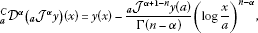
(i)
if , can be represented by
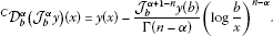
(20)and can be represented by
(21) -
(ii)
if , then
(22)
In particular,
Proof Let . Using the definition of left Hadamard fractional derivative (14) and applying integrating by parts formula and in (16), one gets
Performing once more the integration by parts with the same choice of dv, one gets equation (20). (21) is proved in a similar way. Now, when we have
That is
From Lemma 1.2 in [1], one derives . The second formula in (22) can be proved likewise. □
Theorem 2.2 Letand. If, where. Thenandare continuous onand
-
(i)
if , and can be represented by (20) and (21) respectively and
(24) -
(ii)
if , then the formulas in (22) hold.
Proof The representations (21) and (22) are proved like in Theorem 2.1. The continuity of and results from their representations and Lemma 2.36 in [1] with , and α replaced by . The identities in (24) hold since


When , the first formula in (22) holds as a result of Lemma 1.4 in [1]. The second formula can be proved likewise. □
Corollary 2.3 Letand.
-
(i)
If , then is bounded from the space to the space and is bounded from the space to the space and
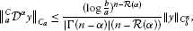 (27)
(27)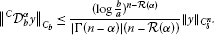 (28)
(28) -
(ii)
If , then and are bounded from to and
(29)


Proof (27) and (28) follow from the estimates (25) and (26) keeping in mind that (see formula 1.1.28 in [1] when ). The estimates in (29) are straightforward. □
and provide operations inverse to and respectively for or . But it is not the case for and .
Lemma 2.4 Let, and.
-
(i)
If or , then
(30) -
(ii)
If and then
 (31)
(31) (32)
(32)


Proof From (16), we have
From properties 2.28 and 2.27 in [1], we have and . It is easy to verify that
from which we conclude that , and thus the first identity in (30) holds. The second identity is proved analogously.
If , , , then and , and similar to (34) we have
Thus we have , and hence (31) holds. (32) can be proved similarly. □
Lemma 2.5 Letorand. Then


Proof (36) and (37) follow from the identities and respectively. □
The Caputo modifications of the left and right Hadamard fractional derivatives have the same properties 2.7.16 and 2.7.18. in [1] but they are different from the ones in 2.7.19.
Property 2.6 Let , and . Then


In particular, one has
Caputo-Hadamard fractional derivatives can also be defined on the positive half axis by replacing a by 0 in formula (20) and b by ∞ in formula (21) provided that (or ). Thus one has


The Mellin transforms of the Caputo modifications of the left and right Hadamard fractional derivatives are the same as Mellin transforms of the left and right Hadamard fractional derivatives 2.7.72 and 2.7.74 in [1].
Lemma 2.7 Letandbe such that the Mellin transforms, exist for.
-
(i)
If , then
(44) -
(ii)
If , then
(45)
Proof (44) follows from Lemma 2.38 and formula 1.4.35 in [1]
(45) can be proved similarly. □
Authors’ information
DB is on leave of absence from Institute of Space Sciences, P.O. Box MG-23, R 76900, Magurele-Bucharest, Romania.
References
Kilbas AA, Srivastava HH, Trujillo JJ: Theory and Applications of Fractional Differential Equations. Elsevier, Amsterdam; 2006.
Samko SG, Kilbas AA, Marichev OI: Fractional Integrals and Derivatives - Theory and Applications. Gordon & Breach, Langhorne; 1993.
Hadamarad J: Essai sur l’etude des fonctions donnes par leur developpment de Taylor. J. Pure Appl. Math. 1892, 4(8):101–186.
Podlubny I: Fractional Differential Equations. Academic Press, San Diego; 1999.
Magin RL: Fractional Calculus in Bioengineering. Begell House Publishers, Redding; 2006.
Heymans N, Podlubny I: Physical interpretation of initial conditions for fractional differential equations with Riemann-Liouville fractional derivatives. Rheol. Acta 2006, 45: 765–771. 10.1007/s00397-005-0043-5
Jesus IS, Machado JAT: Fractional control of heat diffusion system. Nonlinear Dyn. 2008, 54(3):263–282. 10.1007/s11071-007-9322-2
Mainardi F, Luchko Y, Pagnini G: The fundamental solution of the space-time fractional the space-time fractional diffusion equation. Fract. Calc. Appl. Anal. 2001, 4(2):153–192.
Scalas E, Gorenflo R, Mainardi F: Uncoupled continuous-time random walks: solution and limiting behavior of the master equation. Phys. Rev. E 2004., 69: Article ID 011107
Agrawal OP, Baleanu D: Hamiltonian formulation and a direct numerical scheme for fractional optimal control problems. J. Vib. Control 2007, 13(9–10):1269–1281. 10.1177/1077546307077467
Chen YQ, Vinagre BM, Podlubny I: Continued fraction expansion approaches to discretizing fractional order derivatives-an expository review. Nonlinear Dyn. 2004, 38(1–4):155–170. 10.1007/s11071-004-3752-x
Tarasov VE, Zaslavsky GM: Nonholonomic constraints with fractional derivatives. J. Phys. A, Math. Gen. 2006, 39(31):9797–9815. 10.1088/0305-4470/39/31/010
Kilbas AA: Hadamard-type fractional calculus. J. Korean Math. Soc. 2001, 38(6):1191–1204.
Kilbas AA, Titjura AA: Hadamard-type fractional integrals and derivatives. Tr. Inst. Mat., Minsk 2002, 11: 79–87.
Butzer PL, Kilbas AA, Trujillo JJ: Compositions of Hadamard-type fractional integration operators and the semigroup property. J. Math. Anal. Appl. 2002, 269(2):387–400. 10.1016/S0022-247X(02)00049-5
Butzer PL, Kilbas AA, Trujillo JJ: Fractional calculus in Mellin setting and Hadamard-type fractional integrals. J. Math. Anal. Appl. 2002, 269(1):1–27. 10.1016/S0022-247X(02)00001-X
Butzer PL, Kilbas AA, Trujillo JJ: Mellin transformation and integration by parts for Hadamard-type fractional integrals. J. Math. Anal. Appl. 2002, 270(1):1–15. 10.1016/S0022-247X(02)00066-5
Acknowledgement
This work is partially supported by the Scientific and Technical Research Council of Turkey.
Author information
Authors and Affiliations
Corresponding author
Additional information
Competing interests
The authors have no competing interests.
Authors’ contributions
FJ and TA wrote the first version of the manuscript. DB improved it and he prepared the final version of the manuscript. All authors read and approved the final manuscript.
Rights and permissions
Open Access This article is distributed under the terms of the Creative Commons Attribution 2.0 International License ( https://creativecommons.org/licenses/by/2.0 ), which permits unrestricted use, distribution, and reproduction in any medium, provided the original work is properly cited.
About this article
Cite this article
Jarad, F., Abdeljawad, T. & Baleanu, D. Caputo-type modification of the Hadamard fractional derivatives. Adv Differ Equ 2012, 142 (2012). https://doi.org/10.1186/1687-1847-2012-142
Received:
Accepted:
Published:
DOI: https://doi.org/10.1186/1687-1847-2012-142