Controllability results for impulsive mixed-type functional integro-differential evolution equations with nonlocal conditions

Abstract

In this paper, we establish the controllability for a class of abstract impulsive mixed-type functional integro-differential equations with finite delay in a Banach space. Some sufficient conditions for controllability are obtained by using the Mönch fixed point theorem via measures of noncompactness and semigroup theory. Particularly, we do not assume the compactness of the evolution system. An example is given to illustrate the effectiveness of our results.

MSC:93B05, 34A37, 34G20.

1 Introduction

In recent years, the theory of impulsive differential equations has provided a natural framework for mathematical modeling of many real world phenomena, namely in control, biological and medical domains. In these models, the investigated simulating processes and phenomena are subjected to certain perturbations whose duration is negligible in comparison with the total duration of the process. Such perturbations can be reasonably well approximated as being instantaneous changes of state, or in the form of impulses. These processes tend to be more suitably modeled by impulsive differential equations, which allow for discontinuities in the evolution of the state. For more details on this theory and its applications, we refer to the monographs of Bainov and Simeonov [1], Lakshmikantham et al.[2] and Samoilenko and Perestyuk [3] and the papers of [4–12].

On the other hand, the concept of controllability is of great importance in mathematical control theory. The problem of controllability is to show the existence of a control function, which steers the solution of the system from its initial state to the final state, where the initial and final states may vary over the entire space. Many authors have studied the controllability of nonlinear systems with and without impulses; see, for instance, [13–18]. In recent years, significant progress has been made in the controllability of linear and nonlinear deterministic systems [14, 16, 19–24], and the nonlocal initial condition, in many cases, has a much better effect in applications than the traditional initial condition. As remarked by Byszewski and Lakshmikantham (see [25, 26]), the nonlocal initial value problems can be more useful than the standard initial value problems to describe many physical phenomena.

The study of Volterra-Fredholm integro-differential equations plays an important role in abstract formulation of many initial, boundary value problems of perturbed differential partial integro-differential equations. Recently, many authors studied mixed type integro-differential systems without (or with) delay conditions [27–31]. In [16] the controllability of impulsive functional differential systems with nonlocal conditions was studied by using the measures of noncompactness and the Mon̈ch fixed point theorem, and some sufficient conditions for controllability were established. Here, without assuming the compactness of the evolution system, [29] establishes the existence, uniqueness and continuous dependence of mild solutions for nonlinear mixed type integro-differential equations with finite delay and nonlocal conditions. The results are obtained by using the Banach fixed point theorem and semigroup theory.

More recently, Shengli Xie [31] derived the existence of mild solutions for the nonlinear mixed-type integro-differential functional evolution equations with nonlocal conditions, and the results were achieved by using the Mon̈ch fixed point theorem and fixed point theory. Here some restricted conditions on a priori estimates and measures of noncompactness estimation were not used even if the generator $A=0$.

To the best of our knowledge, up to now no work has reported on controllability of an impulsive mixed Volterra-Fredholm functional integro-differential evolution differential system with finite delay, and nonlocal conditions has been an untreated topic in the literature, and this fact is the main aim of the present work.

This paper is motivated by the recent works [16, 29, 31] and its main purpose is to establish sufficient conditions for the controllability of the impulsive mixed-type functional integro-differential system with finite delay and nonlocal conditions of the form

(1.1)

(1.2)

(1.3)

where $A(t)$ is a family of linear operators which generates an evolution system $\{U(t,s):0\le s\le t\le b\}$. The state variable $x(\cdot )$ takes the values in the real Banach space X with the norm $\parallel \cdot \parallel$. The control function $u(\cdot )$ is given in $L^2(J,V)$, a Banach space of admissible control functions with V as a Banach space, and thereby $T=\{(t,s):0\le s\le t\le b\}$. B is a bounded linear operator from V into X. The nonlinear operators $h:T\times \mathcal{D}\to X$, $k:T\times \mathcal{D}\to X$ and $f:J\times \mathcal{D}\times X\times X\to X$ are continuous, where $\mathcal{D}$ = {$\psi :[-r,0]\to X:\psi (t)$ is continuous everywhere except for a finite number of points $t_i$ at which $\psi (t_i^{+})$ and $\psi (t_i^{-})$ exist and $\psi (t_i)=\psi (t_i^{-})$}; $I_i:\mathcal{D}\to X$, $i=1,2,\dots ,s$, are impulsive functions, $0<t_1<t_2<\cdots <t_s<t_{s+1}=b$, $\mathrm{\Delta }\xi (t_i)$ is the jump of a function ξ at $t_i$, defined by $\mathrm{\Delta }\xi (t_i)=\xi (t_i^{+})-\xi (t_i^{-})$.

For any function $x\in \mathcal{PC}$ and any $t\in J$, $x_t$ denotes the function in $\mathcal{D}$ defined by

$$x_t(\theta )=x(t+\theta ),\theta \in [-r,0],$$

where $\mathcal{PC}$ is defined in Section 2. Here $x_t(\cdot )$ represents the history of the state from the time $t-r$ up to the present time t.

Our work is organized as follows. In the next section, fundamental notions and facts related to MNC are recalled. Section 3 is devoted to analyzing controllability results of the problem (1.1)-(1.3). Section 4 contains an illustrative example.

2 Preliminaries

In this section, we recalled some fundamental definitions and lemmas which are required to demonstrate our main results (see [20–24, 32–35]).

Let $L^1([0,b],X)$ be the space of X-valued Bochner integrable functions on $[0,b]$ with the norm ${\parallel f\parallel }_{L^1}={\int }_0^b\parallel f(t)\parallel dt$. In order to define the solution of the problem (1.1)-(1.3), we consider the following space: $\mathcal{PC}([-r,b],X)$ = {$x:[-r,b]\to X$ such that $x(\cdot )$ is continuous except for a finite number of points $t_i$ at which $x(t_i^{+})$ and $x(t_i^{-})$ exist and $x(t_i)=x(t_i^{-})$}.

It is easy to verify that $\mathcal{PC}([-r,b],X)$ is a Banach space with the norm

$${\parallel x\parallel }_{\mathcal{PC}}=sup\{\parallel x(t)\parallel :t\in [-r,b]\}.$$

For our convenience, let $\mathcal{PC}=\mathcal{PC}([-r,b],X)$ and $J_0=[0,t_1]$; $J_i=(t_i,t_{i+1}]$, $i=1,2,\dots ,s$.

Definition 2.1 Let $E^{+}$ be a positive cone of an order Banach space $(E,\le )$. A function Φ defined on the set of all bounded subsets of the Banach space X with values in $E^{+}$ is called a measure of noncompactness (MNC) on X if $\mathrm{\Phi }(\overline{co}\mathrm{\Omega })=\mathrm{\Phi }(\mathrm{\Omega })$ for all bounded subsets $\mathrm{\Omega }\subseteq X$, where $\overline{co}\mathrm{\Omega }$ stands for the closed convex hull of Ω.

The MNC Φ is said to be

• (1) Monotone if for all bounded subsets ${\mathrm{\Omega }}_1$, ${\mathrm{\Omega }}_2$ of X we have $({\mathrm{\Omega }}_1\subseteq {\mathrm{\Omega }}_2)\Rightarrow (\mathrm{\Phi }({\mathrm{\Omega }}_1)\le \mathrm{\Phi }({\mathrm{\Omega }}_2))$;

• (2) Nonsingular if $\mathrm{\Phi }(\{a\}\cup \mathrm{\Omega })=\mathrm{\Phi }(\mathrm{\Omega })$ for every $a\in X$, $\mathrm{\Omega }\subset X$;

• (3) Regular if $\mathrm{\Phi }(\mathrm{\Omega })=0$ if and only if Ω is relatively compact in X.

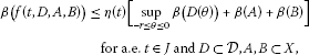
One of the many examples of MNC is the noncompactness measure of Hausdorff β defined on each bounded subset Ω of X by

$$\begin{array}{rcl}\beta (\mathrm{\Omega })& =& inf\{ϵ>0;\mathrm{\Omega }\text{ can be covered by a finite number of balls}\\ \text{of radii smaller than }ϵ\}.\end{array}$$

It is well known that MNC β verifies the above properties and other properties; see [32, 33] for all bounded subsets Ω, ${\mathrm{\Omega }}_1$, ${\mathrm{\Omega }}_2$ of X,

• (4) $\beta ({\mathrm{\Omega }}_1+{\mathrm{\Omega }}_2)\le \beta ({\mathrm{\Omega }}_1)+\beta ({\mathrm{\Omega }}_2)$, where ${\mathrm{\Omega }}_1+{\mathrm{\Omega }}_2=\{x+y:x\in {\mathrm{\Omega }}_1,y\in {\mathrm{\Omega }}_2\}$;

• (5) $\beta ({\mathrm{\Omega }}_1\cup {\mathrm{\Omega }}_2)\le max\{\beta ({\mathrm{\Omega }}_1),\beta ({\mathrm{\Omega }}_2)\}$;

• (6) $\beta (\lambda \mathrm{\Omega })\le |\lambda |\beta (\mathrm{\Omega })$ for any $\lambda \in \mathbb{R}$;

• (7) If the map $Q:D(Q)\subseteq X\to Z$ is Lipschitz continuous with a constant k, then ${\beta }_Z(Q\mathrm{\Omega })\le k\beta (\mathrm{\Omega })$ for any bounded subset $\mathrm{\Omega }\subseteq D(Q)$, where Z is a Banach space.

Definition 2.2 A two-parameter family of bounded linear operators $U(t,s)$, $0\le s\le t\le b$, on X is called an evolution system if the following two conditions are satisfied:

• (i) $U(s,s)=I$, $U(t,r)U(r,s)=U(t,s)$ for $0\le s\le r\le t\le b$;

• (ii) $(t,s)\to U(t,s)$ is strongly continuous for $0\le s\le t\le b$.

Since the evolution system $U(t,s)$ is strongly continuous on the compact operator set $J\times J$, there exists $M_1>0$ such that $\parallel U(t,s)\parallel \le M_1$ for any $(t,s)\in J\times J$. More details about the evolution system can be found in Pazy [34].

Definition 2.3 A function $x(\cdot )\in \mathcal{PC}$ is said to be a mild solution of the system (1.1)-(1.3) if $x(t)=\varphi (t)+g(x)(t)$ on $[-r,0]$, $\mathrm{\Delta }x{|}_{t=t_i}=I_i(x_{t_i})$, $i=1,2,\dots ,s$, the restriction of $x(\cdot )$ to the interval $J_i$ ($i=1,2,\dots ,s$) is continuous and the following integral equation is satisfied.

$$\begin{array}{rcl}x(t)& =& U(t,0)[\varphi (0)+gx(0)]\\ +{\int }_0^{t}U(t,s)[Bu(s)+f(s,x_s,{\int }_0^{s}h(s,\tau ,x_{\tau })d\tau ,{\int }_0^{b}k(s,\tau ,x_{\tau })d\tau )]ds\\ +\sum _{0<t_i<t}U(t,t_i)I_i(x_{t_i}),t\in J.\end{array}$$

Definition 2.4 The system (1.1)-(1.3) is said to be nonlocally controllable on the interval J if, for every initial function $\varphi \in \mathcal{D}$ and $x_1\le X$, there exists a control $u\in L^2(J,V)$ such that the mild solution $x(\cdot )$ of (1.1)-(1.3) satisfies $x(b)=x_1$.

Definition 2.5 A countable set ${\{f_n\}}_{n=1}^{\mathrm{\infty }}\subset L^1([0,b],X)$ is said to be semicompact if the sequence ${\{f_n\}}_{n=1}^{\mathrm{\infty }}$ is relatively compact in X for almost all $t\in [0,b]$, and if there is a function $\mu \in L^1([0,b],{\mathbb{R}}^{+})$ satisfying ${sup}_{n\ge 1}\parallel f_n(t)\parallel \le \mu (t)$ for a.e. $t\in [0,b]$.

Lemma 2.1 (See [32])

If$W\subset C([a,b],X)$is bounded and equicontinuous, then$\beta (W(t))$is continuous for$t\in [a,b]$and

$$\beta (W)=sup\{\beta (W(t)),t\in [a,b]\},\mathit{\text{where}}W(t)=\{x(t):x\in W\}\subseteq X.$$

Lemma 2.2 (See [12])

If$W\subset \mathcal{PC}([a,b],X)$is bounded and piecewise equicontinuous on$[a,b]$, then$\beta (W(t))$is piecewise continuous for$t\in [a,b]$and

$$\beta (W)=sup\{\beta (W(t)),t\in [a,b]\}.$$

Lemma 2.3 (See [19])

Let${\{f_n\}}_{n=1}^{\mathrm{\infty }}$be a sequence of functions in$L^1([0,b],{\mathbb{R}}^{+})$. Assume that there exist$\mu ,\eta \in L^1([0,b],{\mathbb{R}}^{+})$satisfying${sup}_{n\ge 1}\parallel f_n(t)\parallel \le \mu (t)$and$\beta ({\{f_n(t)\}}_{n=1}^{\mathrm{\infty }})\le \eta (t)$a.e. $t\in [0,b]$, then for all$t\in [0,b]$, we have

$$\beta \left(\{{\int }_0^{t}U(t,s)f_n(s)ds:n\ge 1\}\right)\le 2M_1{\int }_0^t\eta (s)ds.$$

Lemma 2.4 (See [19])

Let$(Gf)(t)={\int }_0^{t}U(t,s)f(s)ds$. If${\{f_n\}}_{n=1}^{\mathrm{\infty }}\subset L^1([0,b],X)$is semicompact, then the set${\{G{f}_n\}}_{n=1}^{\mathrm{\infty }}$is relatively compact in$C([0,b],X)$. Moreover, if$f_n\rightharpoonup f_0$, then for all$t\in [0,b]$,

$$(G{f}_n)(t)\to (G{f}_0)(t)\mathit{\text{as}}n\to \mathrm{\infty }.$$

The following fixed-point theorem, a nonlinear alternative of Mon̈ch type, plays a key role in our proof of controllability of the system (1.1)-(1.3).

Lemma 2.5 (See [[35], Theorem 2.2])

Let D be a closed convex subset of a Banach space X and$0\in D$. Assume that$F:D\to X$is a continuous map which satisfies Mon̈ch’s condition, that is, ($M\subseteq D$is countable, $M\subseteq \overline{co}(\{0\}\cup F(M))\Rightarrow \overline{M}$is compact). Then F has a fixed point in D.

3 Controllability results

In this section, we present and demonstrate the controllability results for the problem (1.1)-(1.3). In order to demonstrate the main theorem of this section, we list the following hypotheses.

• (H1) $A(t)$ is a family of linear operators, $A(t):D(A)\to X$, $D(A)$ not depending on t and a dense subset of X, generating an equicontinuous evolution system $\{U(t,s):0\le s\le t\le b\}$, i.e., $(t,s)\to \{U(t,s)x:x\in B\}$ is equicontinous for $t>0$ and for all bounded subsets B and $M_1=sup\{\parallel U(t,s)\parallel :(t,s)\in T\}$.

• (H2) The function $f:J\times \mathcal{D}\times X\times X\to X$ satisfies the following:

  • (i) For $t\in J$, the function $f(t,\cdot ,\cdot ,\cdot ):\mathcal{D}\times X\to X$ is continuous, and for all $(\varphi ,x)\in \mathcal{D}\times X$, the function $f(\cdot ,\varphi ,x,y):J\to X$ is strongly measurable.

  • (ii) For every positive integer $k_1$, there exists ${\alpha }_{k_1}\in L^1([0,b];{\mathbb{R}}^{+})$ such that

    $$\underset{{\parallel \varphi \parallel }_{\mathcal{D}}\le k_1}{sup}\parallel f(t,\varphi )\parallel \le {\alpha }_{k_1}(t)\text{for a.e. }t\in J,$$

    and

    $$\underset{r\to \mathrm{\infty }}{lim}inf{\int }_0^b\frac{{\alpha }_{k_1}(t)}{k_1}dt=\sigma <\mathrm{\infty }.$$

  • (iii) There exists an integrable function $\eta :[0,b]\to [0,\mathrm{\infty })$ such that

    

    where $D(\theta )=\{v(\theta ):v\in D\}$.

• (H3) The function $h:T\times \mathcal{D}\to X$ satisfies the following:

  • (i) For each $(t,s)\in T$, the function $h(t,s,\cdot ):\mathcal{D}\to X$ is continuous, and for each $x\in \mathcal{D}$, the function $h(\cdot ,\cdot ,x):T\to X$ is strongly measurable.

  • (ii) There exists a function $m\in L^1(T,{\mathbb{R}}^{+})$ such that

    $$\parallel h(t,s,x_s)\parallel \le m(t,s){\parallel x_s\parallel }_{\mathcal{D}}.$$

  • (iii) There exists an integrable function $\zeta :T\to [0,\mathrm{\infty })$ such that

    $$\beta (h(t,s,H))\le \zeta (t,s)\underset{-r\le \theta \le 0}{sup}H(\theta )\text{for a.e }t\in J$$

    and $H\subset \mathcal{D}$, where $H(\theta )=\{w(\theta ):w\in H\}$ and β is the Hausdorff MNC.

  For convenience, let us take $L_0=max{\int }_0^{t}m(t,s)ds$ and ${\zeta }^{\ast }=max{\int }_0^s\zeta (t,s)ds$.

• (H4) The function $k:T\times \mathcal{D}\to X$ satisfies the following:

  • (i) For each $(t,s)\in T$, the function $k(t,s,\cdot ):\mathcal{D}\to X$ is continuous, and for each $x\in \mathcal{D}$, the function $k(\cdot ,\cdot ,x):T\to X$ is strongly measurable.

  • (ii) There exists a function $m\in L^1(T,{\mathbb{R}}^{+})$ such that

    $$\parallel k(t,s,x_s)\parallel \le m^{\star }(t,s){\parallel x_s\parallel }_{\mathcal{D}}.$$

  • (iii) There exists an integrable function $\gamma :T\to [0,\mathrm{\infty })$ such that

    $$\beta (k(t,s,H))\le \gamma (t,s)\underset{-r\le \theta \le 0}{sup}H(\theta )\text{for a.e. }t\in J$$

    and $H\subset \mathcal{D}$, where $H(\theta )=\{w(\theta ):w\in H\}$.

  For convenience, let us take $L_1=max{\int }_0^t{m}^{\star }(t,s)ds$ and ${\gamma }^{\ast }=max{\int }_0^s\gamma (t,s)ds$.

• (H5) $g:\mathcal{PC}([0,b]:X)\to X$ is a continuous compact operator such that

  $$\underset{{\parallel y\parallel }_{PC}\to \mathrm{\infty }}{lim}\frac{\parallel g(y)\parallel }{{\parallel y\parallel }_{PC}}=0.$$

• (H6) The linear operator $W:L^2(J,V)\to X$ is defined by

  $$W={\int }_0^{b}U(t,s)Bu(s)ds\text{such that}$$

  • (i) W has an invertible operator $W^{-1}$ which takes values in $L^2(J,V)/kerW$, and there exist positive constants $M_2$ and $M_3$ such that

    $$\parallel B\parallel \le M_2,\parallel W^{-1}\parallel \le M_3.$$

  • (ii) There is $K_W\in L^1(J,{\mathbb{R}}^{+})$ such that, for every bounded set $Q\subset X$,

    $$\beta \left(W^{-1}Q\right)(t)\le K_W(t)\beta (Q).$$

• (H7) $I_i:\mathcal{D}\to X$, $i=1,2,\dots ,s$, is a continuous operator such that

  • (i) There are nondecreasing functions $L_i:{\mathbb{R}}^{+}\to {\mathbb{R}}^{+}$ such that

    $$\parallel I_i(x)\parallel \le L_i\left({\parallel x\parallel }_{\mathcal{D}}\right),i=1,2,\dots ,s,x\in \mathcal{D},$$

    and

    $$\underset{\rho \to \mathrm{\infty }}{lim}inf\frac{L_i(\rho )}{\rho }={\lambda }_i<\mathrm{\infty },i=1,2,\dots ,s.$$

  • (ii) There exist constants $K_i\ge 0$ such that

    $$\beta (I_i(S))\le K_i\underset{-r\le \theta \le 0}{sup}\beta (S(\theta )),i=1,2,\dots ,s,$$

    for every bounded subset S of $\mathcal{D}$.

• (H8) The following estimation holds true:

  $$\begin{array}{rcl}N& =& [(M_1+2M_1^2{M}_2{\parallel K_W\parallel }_{L^1})\sum _{i=1}^s{K}_i\\ +[1+2({\zeta }^{\ast }+{\gamma }^{\ast })](2M_1+4M_1^2{M}_2{\parallel K_W\parallel }_{L^1}){\parallel \eta \parallel }_{L^1}]<1.\end{array}$$

Theorem 3.1 Assume that the hypotheses (H1)-(H8) are satisfied. Then the impulsive differential system (1.1)-(1.3) is controllable on J provided that

$$M_1(1+M_1{M}_2{M}_3{b}^{\frac{1}{2}})[\sigma (1+L_0+L_1)]+\sum _{i=1}^s{\lambda }_i<1.$$

(3.1)

Proof Using the hypothesis (H6)(i), for every $x\in \mathcal{PC}([-r,b],X)$, define the control

$$\begin{array}{rcl}{u}_x(t)& =& W^{-1}[x_1-U(b,0)\phi (0)-{\int }_0^{b}U(b,s)\\ \times f(s,x_s,{\int }_0^{s}h(s,\tau ,x_{\tau })d\tau ,{\int }_0^{b}k(s,\tau ,x_{\tau })d\tau )ds-\sum _{0<t_i<b}U(b,t_i)I_i(x_{t_i})](t).\end{array}$$

We shall now show that when using this control, the operator defined by

$$(Fx)(t)=\{\begin{array}{c}\varphi (t),t\in [-r,0],\hfill \\ U(t,0)[\varphi (0)+gx(0)]+{\int }_0^{t}U(t,s)\hfill \\ \times [f(s,x_s,{\int }_0^{t}h(t,\tau ,x_{\tau })d\tau ,{\int }_0^{b}k(s,\tau ,x_{\tau })d\tau )ds+(B{u}_x)(s)]ds\hfill \\ +{\sum }_{0<t_i<t}U(t,t_i)I_i(x_{t_i}),t\in J,\hfill \end{array}$$

has a fixed point. This fixed point is then a solution of (1.1)-(1.3). Clearly, $x(b)=(Fx)(b)=x_1$, which implies the system (1.1)-(1.3) is controllable. We rewrite the problem (1.1)-(1.3) as follows.

For $\varphi \in \mathcal{D}$, we define $\hat{\varphi }\in \mathcal{PC}$ by

$$\hat{\varphi }(t)=\{\begin{array}{cc}U(t,0)[\varphi (0)+gx(0)],\hfill & t\in J,\hfill \\ \varphi (t),\hfill & t\in [-r,0].\hfill \end{array}$$

Then $\hat{\varphi }\in \mathcal{PC}$. Let $x(t)=y(t)+\hat{\varphi }(t)$, $t\in [-r,b]$. It is easy to see that y satisfies $y_0=0$ and

$$\begin{array}{rcl}y(t)& =& {\int }_0^{t}U(t,s)\\ \times [f(s,y_s+{\hat{\varphi }}_s,{\int }_0^{s}h(s,\tau ,y_{\tau }+{\hat{\varphi }}_{\tau })d\tau ,{\int }_0^{s}k(s,\tau ,y_{\tau }+{\hat{\varphi }}_{\tau })d\tau )+B{u}_y(s)]ds\\ +\sum _{0<t_i<t}U(t,t_i)I_i(y_{t_i}+{\hat{\varphi }}_{t_i}),\end{array}$$

where

$$\begin{array}{rcl}{u}_y(s)& =& W^{-1}[x_1-U(b,0)[\varphi (0)+gx(0)]\\ -{\int }_0^{b}U(b,s)f(s,y_s+{\hat{\varphi }}_s,{\int }_0^{s}h(s,\tau ,y_{\tau }+{\hat{\varphi }}_{\tau })d\tau ,{\int }_0^{b}k(s,\tau ,y_{\tau }+{\hat{\varphi }}_{\tau })d\tau )ds\\ -\sum _{i=1}^{s}U(b,t_i)I_i(y_{t_i}+{\hat{\varphi }}_{t_i})](s)\end{array}$$

if and only if x satisfies

$$\begin{array}{rcl}x(t)& =& U(t,0)[\varphi (0)+gx(0)]\\ +{\int }_0^{t}U(t,s)[f(s,x_s,{\int }_0^{s}h(s,\tau ,x_{\tau })d\tau ,{\int }_0^{b}k(s,\tau ,x_{\tau })d\tau )+B{u}_x(s)]ds\\ +\sum _{0<t_i<t}U(t,t_i)I_i(x_{t_i}),\end{array}$$

and $x(t)=\varphi (t)+gx(t)$, $t\in [-r,0]$. Define ${\mathcal{PC}}_0=\{y\in \mathcal{PC}:y_0=0\}$. Let $G:{\mathcal{PC}}_0\to {\mathcal{PC}}_0$ be an operator defined by

$$(Gy)(t)=\{\begin{array}{c}0,t\in [-r,0],\hfill \\ {\int }_0^{t}U(t,s)[f(s,y_s+{\hat{\varphi }}_s,{\int }_0^{s}h(s,\tau ,y_{\tau }+{\hat{\varphi }}_{\tau })d\tau ,\hfill \\ {\int }_0^{b}k(s,\tau ,y_{\tau }+{\hat{\varphi }}_{\tau })d\tau )+B{u}_y(s)]ds\hfill \\ +{\sum }_{0<t_i<t}U(t,t_i)I_i(y_{t_i}+{\hat{\varphi }}_{t_i}),t\in J.\hfill \end{array}$$

(3.2)

Obviously, the operator F has a fixed point is equivalent to G has one. So, it turns out to prove G has a fixed point. Let $G=G_1+G_2$, where

(3.3)

(3.4)

Step 1: There exists a positive number $q\ge 1$ such that $G(B_q)\subseteq B_q$, where $B_q=\{y\in {\mathcal{PC}}_0:{\parallel y\parallel }_{\mathcal{PC}}\le q\}$.

Suppose the contrary. Then for each positive integer q, there exists a function $y^q(\cdot )\in B_q$ but $G(y^q)\notin B_q$, i.e., $\parallel G(y^q)(t)\parallel >q$ for some $t\in J$.

We have from (H1)-(H7)

$$\begin{array}{rcl}q& <& \parallel \left(G{y}^q\right)(t)\parallel \\ \le & M_1{\int }_0^b\parallel f(s,y_s^q+{\hat{\varphi }}_s,{\int }_0^{s}h(s,\tau ,y_{\tau }^q+{\hat{\varphi }}_{\tau })d\tau ,{\int }_0^{b}k(s,\tau ,y_{\tau }^q+{\hat{\varphi }}_{\tau })d\tau )+B{u}_{y^q}(s)\parallel ds\\ +M_1\sum _{i=1}^s{L}_i\left({\parallel y_{t_i}^q+{\hat{\varphi }}_{t_i}\parallel }_{\mathcal{D}}\right).\end{array}$$

Since

where, $q^{\ast }=(1+L_0)q^{\mathrm{\prime }}$ and $q^{\mathrm{\prime }}=q+{\parallel \hat{\varphi }\parallel }_{\mathcal{PC}}$, we have

$$q\le M_1{\int }_0^b{\alpha }_{q^{\ast }}(s)ds+M_1{M}_2{b}^{\frac{1}{2}}{\parallel u_{y^q}\parallel }_{L^2}+M_1\sum _{i=1}^s{L}_i\left(q^{\mathrm{\prime }}\right),$$

(3.5)

where

$${\parallel u_{y^q}\parallel }_{L^2}\le M_3[\parallel x_1\parallel +M_1{\parallel \varphi \parallel }_{\mathcal{D}}+M_1{\int }_0^b{\alpha }_{q^{\ast }}(s)ds+M_1\sum _{i=1}^s{L}_i\left(q^{\mathrm{\prime }}\right)].$$

(3.6)

Hence by (3.5)

$$\begin{array}{rcl}q& <& M_1{\int }_0^b{\alpha }_{q^{\ast }}(s)ds+M_1{M}_2{b}^{\frac{1}{2}}{M}_3[\parallel x_1\parallel +M_1{\parallel \varphi \parallel }_{\mathcal{D}}+M_1{\int }_0^b{\alpha }_{q^{\ast }}(s)ds+M_1\sum _{i=1}^s{L}_i\left(q^{\mathrm{\prime }}\right)]\\ +M_1\sum _{i=1}^s{L}_i\left(q^{\mathrm{\prime }}\right)\\ \le & (1+M_1{M}_2{M}_3{b}^{\frac{1}{2}})M_1[{\int }_0^b{\alpha }_{q^{\ast }}(s)ds+\sum _{i=1}^s{L}_i\left(q^{\mathrm{\prime }}\right)]+M,\end{array}$$

where $M=M_1{M}_2{M}_3{b}^{\frac{1}{2}}(\parallel x_1\parallel +M_1{\parallel \varphi \parallel }_{\mathcal{D}})$ is independent of q and $q^{\mathrm{\prime }}=q+{\parallel \hat{\varphi }\parallel }_{\mathcal{PC}}$.

Dividing both sides by q and noting that $q^{\mathrm{\prime }}=q+{\parallel \hat{\varphi }\parallel }_{\mathcal{PC}}\to \mathrm{\infty }$ as $q\to \mathrm{\infty }$, we obtain

Thus we have

$$1\le M_1(1+M_1{M}_2{M}_3{b}^{\frac{1}{2}})(\sigma (1+L_0+L_1)+\sum _{i=1}^s{\lambda }_i).$$

This contradicts (3.1). Hence, for some positive number q, $G(B_q)\subseteq B_q$.

Step 2: $G:{\mathcal{PC}}_0\to {\mathcal{PC}}_0$ is continuous.

Let ${\{y^{(n)}(t)\}}_{n=1}^{\mathrm{\infty }}\subseteq {\mathcal{PC}}_0$ with $y^{(n)}\to y$ in ${\mathcal{PC}}_0$. Then there is a number $q>0$ such that $\parallel y^{(n)}(t)\parallel \le q$ for all n and $t\in J$, so $y^{(n)}\in B_q$ and $y\in B_q$.

From (H2) and (H5) we have

• (i)
  

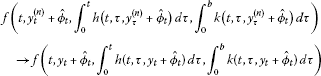
and

(ii) $I_i(y_{t_i}^{(n)}+{\hat{\varphi }}_{t_i})\to I_i(y_{t_i}+{\hat{\varphi }}_{t_i})$, $i=1,2,\dots ,s$.

Then we have

$${\parallel G_1{y}^{(n)}-G_{1}y\parallel }_{\mathcal{PC}}\le \sum _{i=1}^s\parallel I_i(y_{t_i}^{(n)}+{\hat{\varphi }}_{t_i})-I_i(y_{t_i}+{\hat{\varphi }}_{t_i})\parallel$$

(3.7)

and

(3.8)

where

(3.9)

Observing (3.7)-(3.9), by the dominated convergence theorem, we have that

$${\parallel G{y}^{(n)}-Gy\parallel }_{\mathcal{PC}}\le {\parallel G_1{y}^{(n)}-Gy\parallel }_{\mathcal{PC}}+{\parallel G_2{y}^{(n)}-G_{2}y\parallel }_{\mathcal{PC}}\to 0\text{as }n\to +\mathrm{\infty }.$$

That is, G is continuous.

Step 3: G is equicontinuous on every $J_i$, $i=1,2,\dots ,s$. That is, $G(B_q)$ is piecewise equicontinuous on J.

Indeed, for $t_1,t_2\in J_i$, $t_1<t_2$ and $y\in B_q$, we deduce that

(3.10)

By the equicontinuity of $U(\cdot ,s)$ and the absolute continuity of the Lebesgue integral, we can see that the right-hand side of (3.10) tends to zero and is independent of y as $t_2\to t_1$. Hence $G(B_q)$ is equicontinuous on $J_i$ ($i=1,2,\dots ,s$).

Step 4: Mon̈ch’s condition holds.

Suppose $W\subseteq B_q$ is countable and $W\subseteq \overline{co}(\{0\}\cup G(W))$. We shall show that $\beta (W)=0$, where β is the Hausdorff MNC.

Without loss of generality, we may assume that $W={\{y^{(n)}\}}_{n=1}^{\mathrm{\infty }}$. Since G maps $B_q$ into an equicontinuous family, $G(W)$ is equicontinuous on $J_i$. Hence $W\subseteq \overline{co}(\{0\}\cup G(W))$ is also equicontinuous on every $J_i$.

By (H7)(ii) we have

(3.11)

By Lemma 2.3 and from (H3)(iii), (H4)(iii), (H6)(ii) and (H7)(ii), we have that

(3.12)

This implies that

(3.13)

From (3.11) and (3.13) we obtain that

(3.14)

for each $t\in J$.

Since W and $G(W)$ are equicontinuous on every $J_i$, according to Lemma 2.2, the inequality (3.14) implies that

That is, $\beta (GW)\le N\beta (W)$, where N is defined in (H8). Thus, from Mon̈ch’s condition, we get that

$$\beta (W)\le \beta (\overline{co}(\{0\}\cup G(W))=\beta (G(W))\le N\beta (W)$$

since $N<1$, which implies that $\beta (W)=0$. So, we have that W is relatively compact in ${\mathcal{PC}}_0$. In the view of Lemma 2.5, i.e., Mon̈ch’s fixed point theorem, we conclude that G has a fixed point y in W. Then $x=y+\hat{\varphi }$ is a fixed point of F in $\mathcal{PC}$, and thus the system (1.1)-(1.3) is nonlocally controllable on the interval $[0,b]$. This completes the proof. □

Here we must remark that the conditions (H1)-(H8) given above are at least sufficient, because it is an open problem to prove that they are also necessary or to find an example which points out clearly that the mentioned conditions are not necessary to get the main result proved in this section.

4 An example

Consider the partial functional integro-differential systems with impulsive conditions of the form

(4.1)

(4.2)

(4.3)

(4.4)

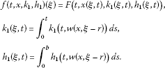
where $r>0$, $I_i>0$, $i=1,2,\dots ,s$, $\phi \in \mathcal{D}$ = {$\psi :[-r,b]\times [0,\pi ]\to \mathbb{R}$, ψ is continuous everywhere except for a countable number of points at which $\psi (s^{-})$, $\psi (s^{+})$ exist with $\psi (s^{-})=\psi (s)$}, $0=t_0<t_1<t_2<\cdots <t_{s+1}=b$, $z(t_i^{+})={lim}_{(h,\xi )\to (0^{+},\xi )}z(t_i+h,\xi )$, $z(t_i^{-})={lim}_{(h,\xi )\to (0^{-},\xi )}z(t_i+h,\xi )$, $B:X\to X$.

Let $X=L^2[0,\pi ]$ and $A(t)\equiv A:X\to X$ be defined by $Aw=w^{\prime }$ with the domain $D(A)=\{w\in X:w\text{ is absolutely continuous }{w}^{\mathrm{\prime }}\in X\text{, }w(\xi )=w(0)=0\}$. It is well known that A is an infinitesimal generator of a semigroup $T(t)$ defined by $T(t)w(s)=w(t+s)$ for each $w\in X$. $T(t)$ is not a compact semigroup on X and $\beta (T(t)D)\le \beta (D)$, where β is the Hausdorff MNC. We also define the bounded linear control operator $B:X\to X$ by

$$(Bu)(\xi )=m(\xi )u(\xi )\text{for almost every }\xi \in [0,\pi ].$$

We assume that

• (1) $f:[0,b]\times X\times X\times X\to X$ is a continuous function defined by

  

  We take $F(t,x(\xi ,t),k_1(\xi ,t),h_1(\xi ,t))=C_{0}sin(x(\xi ))$, $C_0$ is a constant. F is Lipschitz continuous for the second variable. Then f satisfies the hypotheses (H2) and (H3) of Section 3.

• (2) $I_i:X\to X$ is a continuous function for each $i=1,2,\dots ,s$ defined by

  $$I_i(x)(\xi )=I_i(x(\xi )).$$

  We take $I_i(x)(\xi )={\int }_{[0,\pi ]}{\rho }_i(\xi ,y){cos}^2(x(y))dy$, $x\in X$, ${\varphi }_i\in C([0,\pi ]\times [0,\pi ],R)$, for each $i=1,2,\dots ,s$. Then $I_i$ is compact and satisfies the hypothesis (H6)(i).

• (3) $g:\mathcal{PC}([0,b]:X)\to X$ is a continuous function defined by

  $$g(\phi )(\xi )={\int }_0^{b}h(s)log(1+|\phi (s)(\xi )|)ds,\phi \in PC([0,b]:X)$$

  with $\phi (s)(\xi )=z(s,\xi )$. Then g is a compact operator and satisfies the hypothesis (H5).

Therefore, the above partial differential system (4.1)-(4.4) can be written to the abstract form (1.1)-(1.3) and all conditions of Theorem 3.1 are satisfied. We can conclude that the system (4.1)-(4.4) is nonlocally controllable on the interval J.

Conclusions

In the current paper, we are focused on finding some sufficient conditions to establish controllability results for a class of impulsive mixed-type functional integro-differential equations with finite delay. The proof of the main theorem is based on the application of the Mon̈ch fixed point theorem with a noncompact condition of the evolution system. An example is also included to illustrate the technique.

References

Bainov DD, Simeonov PS: Impulsive Differential Equations: Periodic Solutions and Applications. Longman, Harlow; 1993.
Lakshmikantham V, Bainov DD, Simeonov PS: Theory of Impulsive Differential Equations. World Scientific, Singapore; 1989.
Samoilenko AM, Perestyuk NA: Impulsive Differential Equations. World Scientific, Singapore; 1995.
Balachandran K, Annapoorani N: Existence results for impulsive neutral evolution integrodifferential equations with infinite delay. Nonlinear Anal. 2009, 3: 674–684.
Benchohra M, Henderson J, Ntouyas SK: Existence results for impulsive multivalued semilinear neutral functional inclusions in Banach spaces. J. Math. Anal. Appl. 2001, 263: 763–780. 10.1006/jmaa.2001.7663
Fan Z: Impulsive problems for semilinear differential equations with nonlocal conditions. Nonlinear Anal. 2010, 72: 1104–1109. 10.1016/j.na.2009.07.049
Hernandez E, Rabello M, Henriquez H: Existence of solutions for impulsive partial neutral functional differential equations. J. Math. Anal. Appl. 2007, 331: 1135–1158. 10.1016/j.jmaa.2006.09.043
Ji S, Li G: Existence results for impulsive differential inclusions with nonlocal conditions. Comput. Math. Appl. 2011, 62: 1908–1915. 10.1016/j.camwa.2011.06.034
Sivasankaran S, Mallika Arjunan M, Vijayakumar V: Existence of global solutions for second order impulsive abstract partial differential equations. Nonlinear Anal. TMA 2011,74(17):6747–6757. 10.1016/j.na.2011.06.054
Vijayakumar V, Sivasankaran S, Mallika Arjunan M: Existence of global solutions for second order impulsive abstract functional integrodifferential equations. Dyn. Contin. Discrete Impuls. Syst. 2011, 18: 747–766.
Vijayakumar V, Sivasankaran S, Mallika Arjunan M: Existence of solutions for second-order impulsive neutral functional integro-differential equations with infinite delay. Nonlinear Stud. 2012,19(2):327–343.
Ye R: Existence of solutions for impulsive partial neutral functional differential equation with infinite delay. Nonlinear Anal. 2010, 73: 155–162. 10.1016/j.na.2010.03.008
Chang YK, Anguraj A, Mallika Arjunan M: Controllability of impulsive neutral functional differential inclusions with infinite delay in Banach spaces. Chaos Solitons Fractals 2009,39(4):1864–1876. 10.1016/j.chaos.2007.06.119
Chen L, Li G: Approximate controllability of impulsive differential equations with nonlocal conditions. Int. J. Nonlinear Sci. 2010, 10: 438–446.
Guo M, Xue X, Li R: Controllability of impulsive evolution inclusions with nonlocal conditions. J. Optim. Theory Appl. 2004, 120: 355–374.
Ji S, Li G, Wang M: Controllability of impulsive differential systems with nonlocal conditions. Appl. Math. Comput. 2011, 217: 6981–6989. 10.1016/j.amc.2011.01.107
Li M, Wang M, Zhang F: Controllability of impulsive functional differential systems in Banach spaces. Chaos Solitons Fractals 2006, 29: 175–181. 10.1016/j.chaos.2005.08.041
Selvi S, Mallika Arjunan M: Controllability results for impulsive differential systems with finite delay. J. Nonlinear Sci. Appl. 2012, 5: 206–219.
Obukhovski V, Zecca P: Controllability for systems governed by semilinear differential inclusions in a Banach space with a noncompact semigroup. Nonlinear Anal. 2009, 70: 3424–3436. 10.1016/j.na.2008.05.009
Klamka J: Schauders fixed-point theorem in nonlinear controllability problems. Control Cybern. 2000,29(1):153–165.
Klamka J: Constrained approximate controllability. IEEE Trans. Autom. Control 2000,45(9):1745–1749. 10.1109/9.880640
Klamka J: Constrained controllability of semilinear delayed systems. Bull. Pol. Acad. Sci., Tech. Sci. 2001,49(3):505–515.
Klamka J: Constrained controllability of semilinear systems. Nonlinear Anal. 2001, 47: 2939–2949. 10.1016/S0362-546X(01)00415-1
Klamka J: Constrained exact controllability of semilinear systems. Syst. Control Lett. 2002,4(2):139–147.
Byszewski L: Theorems about existence and uniqueness of solutions of a semi-linear evolution nonlocal Cauchy problem. J. Math. Anal. Appl. 1991, 162: 494–505. 10.1016/0022-247X(91)90164-U
Byszewski L, Lakshmikantham V: Theorem about the existence and uniqueness of a solution of a nonlocal abstract Cauchy problem in a Banach space. Appl. Anal. 1991, 40: 11–19. 10.1080/00036819008839989
Anguraj A, Karthikeyan P, Trujillo JJ: Existence of solutions to fractional mixed integro-differential equations with nonlocal initial condition. Adv. Differ. Equ. 2011. doi:10.1155/2011/690653
Chang YK, Chalishajar DN: Controllability of mixed Volterra-Fredholm type integro-differential inclusions in Banach spaces. J. Franklin Inst. 2008, 345: 499–507. 10.1016/j.jfranklin.2008.02.002
Dhakne MB, Kucche KD: Existence of a mild solution of mixed Volterra-Fredholm functional integro-differential equation with nonlocal condition. Appl. Math. Sci. 2011,5(8):359–366.
Ntouyas SK, Purnaras IK: Existence results for mixed Volterra-Fredholm type neutral functional integro-differential equations in Banach spaces. Nonlinear Stud. 2009,16(2):135–148.
Xie S: Existence of solutions for nonlinear mixed type integro-differential functional evolution equations with nonlocal conditions. Abstr. Appl. Anal. 2012. doi:10.1155/2012/913809
Banas J, Goebel K Lecture Notes in Pure and Applied Mathematics. In Measure of Noncompactness in Banach Spaces. Dekker, New York; 1980.
Kamenskii M, Obukhovskii V, Zecca P: Condensing Multivalued Maps and Semilinear Differential Inclusions in Banach Spaces. De Gruyter, Berlin; 2001.
Pazy A: Semigroups of Linear Operators and Applications to Partial Differential Equations. Springer, New York; 1983.
Mon̈ch H: Boundary value problems for nonlinear ordinary differential equations of second order in Banach spaces. Nonlinear Anal. 1980, 4: 985–999. 10.1016/0362-546X(80)90010-3
Acknowledgements
Dedicated to Professor Hari M Srivastava.
The work is partially supported by project MTM2010-16499 from the Government of Spain.
Author information
Authors and Affiliations
Corresponding author
Additional information
Competing interests
The authors declare that they have no competing interests.
Authors’ contributions
All authors contributed equally to the manuscript and typed, read, and approved the final manuscript.
Rights and permissions
Open Access This article is distributed under the terms of the Creative Commons Attribution 2.0 International License (https://creativecommons.org/licenses/by/2.0), which permits unrestricted use, distribution, and reproduction in any medium, provided the original work is properly cited.
About this article
Cite this article
Machado, J.A., Ravichandran, C., Rivero, M. et al. Controllability results for impulsive mixed-type functional integro-differential evolution equations with nonlocal conditions. Fixed Point Theory Appl 2013, 66 (2013). https://doi.org/10.1186/1687-1812-2013-66
Received:
Accepted:
Published:
DOI: https://doi.org/10.1186/1687-1812-2013-66