
Abstract
Combined predictive modelling approach that couples the 2D far-field model and the 3D near-field computational fluid dynamic model has been developed to compare the performance of different turbulence models in predicting the flow kinematics around an open offshore intake structure. The k–epsilon (k–ε), k–ε renormalized group (RNG), k–omega (k–ω) and large eddy simulation (LES) models are used in this study. The objective is to select an appropriate turbulence model for simulating the flow field around the open offshore intake. The simulated water level and current speed of these turbulence models were compared with the field sampling results obtained at the vicinity of an existing open offshore intake structure located in the Penang Strait of Malaysia. Through the analysis, it can be concluded that the simulated water level for all turbulence models are broadly consistent with the major trend of measured values with k–ε model reporting the best performance. Comparison of the simulated current speed with the field measurements show that the k–ε RNG model fits better than the other models. The analysis reveals that the LES model has slightly lower accuracy in predicting current speed around the existing intake structure.
1 Introduction
Seawater intake structures are often used by coastal power plants and desalination plants to draw in ambient seawater with certain quality characteristics which are required for specific functions. Thermal power plants required large volumes of water to refrigerate the circuit, while desalination plants turn seawater into drinking water. Constructing seawater intake structures is a major aspect of engineering works, forming a significant proportion of capital costs for these projects’. They may also present the area of greatest risk for such projects. In order to design the seawater intake structure, it is necessary to understand the flow field characteristics around the structure. The impact of the water extraction will be minimized if the suction velocity is low. Fishes may be able to swim away from the intake to avoid impingement or entrainment [1]. Furthermore, where greater turbulence forms around the intake structure, larger amounts of sediment from the seabed will be sucked up—causing siltation problems in the seawater intake system [2]. Johnson [3] presents an overview of the parameters to be considered in the design of hydropower intakes and highlighted that the sediments are one of the major design factors in the intake design.
Various studies have been conducted and indicated that the flow field influnces the sediment transport rate. Khanarmuei et al. [4] experimentally investigated the effect of vortex formation on sediment transport at dual pipe intakes and concluded that the rate of transported sediment was increased by increasing the strength of formed vortex. Moghadam et al. [5] conducted experimental tests to investigate the sediment entry into water intakes. Results showed that the sediment delivery ratio is depends on the main channel Froude number. They also indicated that the sediment delivery ratio is minimum when the Froude number is between 0.35 and 0.45. Emamgholizadeh and Torabi [6] performed an experimental investigation to study the effects of submerged vanes in the exclusion of inflow sediment to the water intakes. Their results indicated that the submerged vanes have effectively limited the inflow bed and suspended load sediments into the water intakes. They also asserted that the combination of vane-induced circulation and streamwise velocity will cause helical flow created by the vortex at the downstream of the vanes, resulting in sediment transport in a direction transverse to the flow direction.
With the advancement in computational modelling techniques, 3D Computational Fluid Dynamics (CFD) models have been successfully tested and utilized to explain the fundamental principles of the flow turbulence generated by the intake structures. Karami et al. [7] utilized the FLOW3D CFD model code to simulate flow patterns at rectangular lateral intake with different dike and submerged vane scenarios. They evaluated three turbulence models: k–ε, RNG and k–ω, with laboratory experiments and indicated that RNG model provides more accurate results. Sefidkoohi et al. [8] examined five turbulence models: Prandtl mixing length, Turbulent energy, k–ε, RNG and LES, in the simulation of flow pattern in a lateral intake. By comparing the results of these numerical predictions to laboratory observations, they concluded that the RNG model has the highest precision, whilst the LES model has the lowest accuracy in predicting the flow field around the intake structure. Tataroglu [9] investigated the vortex formation in a horizontal water intake structure composed of a reservoir-pipe system. They claimed that RNG model did not yield reasonable results. He asserted that RNG model is not suitable to be used in low-intensity turbulence flows due to the dissipative effect of RANS model. He compared the LES model with laminar model and concluded that LES model is better in capturing the vorticity generated close to the sidewalls. Ruether et al. [10] numerically investigated the flow field and the sediment transport at the Kapunga water intake in Tanzania using the k–ε model to predict the turbulence. Yeganeh-Bakhtiary et al. [11] employed the RANS equations, closured with k–ε turbulence model for a fluid phase of a Euler–Lagrange coupling two-phase flow model to investigate the current-induced live-bed scour beneath marine pipelines. Gonzalo et al. [12] conducted a case study in hydro-combined power stations to identify the capabilities and limitations of two turbulence models: RNG and LES for predicting the discharge flow, averaged depth of water, pressures averages, and discharge flow for engineering purposes. They observed that both RNG and LES turbulence models can provide sufficient representations of generic hydraulic performance for the power station operating in spillway mode. Cheng and Ying [13] performed a series of 3D numerical simulation based on the k–ε turbulence model. They investigated the flow characteristics of the eclipsed form arrangement and the March-past method for water intake-outlet arrangement in power plants. Their simulation results are in basic agreement with those of the previous experiments. Zhao and Nohmi [14] used the LES model instead of RANS turbulence model for simulating free water surface flow in pump intakes. They observed that the LES model can capture the peak of circular velocity around the vortex core and that the results show good agreement with experimental observations. Lucino and Gonzalo Dur [15] conducted a study to verify the ability of a commercial CFD code to predict the formation of vortices in a pump sump. They used the LES model, claiming that other turbulence models do not realistically represent the highly unstable and intermittent phenomena involved. Lu et al. [16] conducted a comparative study of turbulence models by simulating separation processes for inorganic suspended solids (ISS) with different particle sizes in a vortex-type grit chamber. Among the k–ε RNG, Real k–ε and Shear Stress Transmission (SST) k–ω turbulence models, they concluded that the k–ε RNG model agreed well with the experimental results for particles with d ≤ 200 µm. However, for particle size that exceeded 200 µm, the Real k–ε model provided the best results. Catalano et al. [17] provided evidence to show that the LES model is more accurate than the RANS model for unsteady flow with Reynolds numbers between 0.5 × 10⁶ and 1 × 10⁶. However, it is worth noting that their computational solutions are inaccurate at higher Reynolds numbers and the Reynolds number dependence is not captured in their study. RANS models can reduce the computational costs by solving the statistically averaged equation system and are most widely used nowadays [18]. Kaheh et al. [19] concluded that the k–ε RNG model is more accurate for predicting issues arising where shear forces are too high, as compared to the k–ε model. Their findings bear a close resemblance to the findings published by Yakhot and Smith [20] which showed that the RNG model presents more accurately for flows with strong shear regions and low-intensity turbulence flows.
The principal goal in examining the flow kinematics is in understanding the accuracy of the simulated flow turbulence generated around the open offshore intake. It is proven that the accuracy of flow turbulence simulation is influenced by different turbulence models. Unfortunately, there is no single turbulence model accepted as superior for all types of problems. This study was carried out to compare the performance of different turbulence models in predicting the flow kinematics around an open offshore intake structure. Four turbulence models, namely the standard k–epsilon (k–ε), k–ε renormalized group (RNG), k–omega (k–ω) and Large Eddy Simulation (LES) models were tested in this study. Water level and current speed predicted by these turbulence models were compared with the field measurement results. From the analysis of various turbulence models, a turbulence model which is suitable to be applied for flow field simulation around the open offshore intake structure was selected.
2 Methodology
This study combined predictive modelling approaches that utilize the Delft3D far-field model and the FLOW3D near-field CFD model. The Delft3D far-field model was used to model the hydrodynamic conditions from the far-field which covered up to few kilometers away. The hydrodynamic results from the far-field model will be used as the boundary condition to the FLOW3D near-field CFD model. This coupled modelling approach can use the simulated far-field ambient conditions in the near-field computations to accurately determine the flow kinematics around the intake structure.
2.1 Field measurement for model validation
To validate the models used in this study, field measurements were conducted around an existing open offshore intake located in the Penang Strait of Malaysia. The intake structure was used to draw ambient seawater for power plant usage. Field measurement has the advantage of being able to observe the outcome in a natural setting rather than in a contrived laboratory environment [21]. Data screening and checking will however be conducted to ensure the consistency and reliability. The following field measurements were conducted:
-
Bathymetric survey
Bathymetric survey was conducted to capture the bed level around the intake structure. The survey covered 2 km alongshore distance and extending 1.3 km seaward as shown in Fig. 1. The survey line is taken at 50 m intervals with a spot interval of 10 m. Three cross-check lines were also measured to ensure consistency of the bathymetric data. The bathymetric survey was conducted by using echo-sounder to determine the water depth by transmitting sound waves into the water and measuring the travel time of the echo to return from the bottom of the water. The echo-sounder was calibrated with the bar check which enables the echo sounder to be set correctly for the sound velocity.
Fig. 1 
Bathymetric survey coverage
-
Water level and current measurements
Water level and current measurements were conducted at 4 locations as shown in Fig. 2. The measurements were carried out by deploying an Acoustic Doppler Current Profiler (ADCP) to capture the data at 10-min intervals. ADCP uses the Doppler effect to measure current velocity profiles in the water column. It transmits the sound at a fixed frequency and then listening to the echo returning from sound scattering in the water, to determine the velocity and depth. ADCP1 which was located approximately 450 m from the intake structure was used for 2D far-field model validation. It was measured from 7th to 21st July 2017 for successive 14 days to cover spring and neap tides. ADCP2, ADCP3 and ADCP4 which were located approximately 2 m, 1 m and 0.5 m respectively from the intake structure, were used for 3D near-field CFD model validation. It measured from 7 to 16th July 2017 to cover high and low tides.
Fig. 2 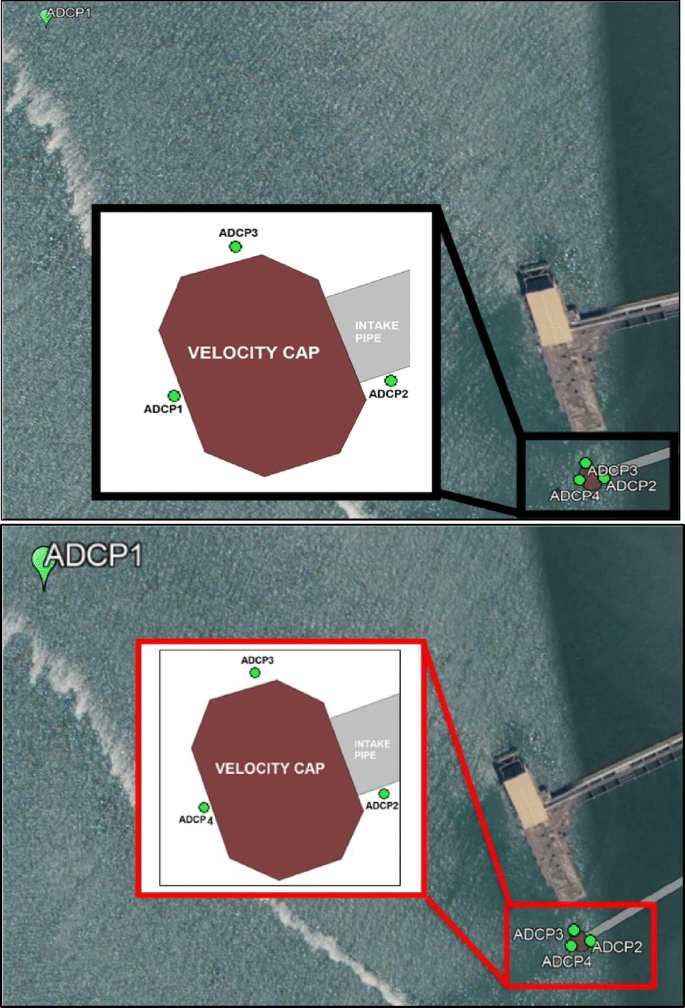
Location for water level and current measurements


2.2 Delft3D
Far-field modelling is performed by using the Delft3D modelling system to simulate hydrodynamic processes due to tides and coastal currents. The Delft3D modelling suite comprises several modules (the details of this model are explained in detailed by Lesser et al. [22]). In this study, the FLOW module was utilized to perform simulation of hydrodynamic flow under the shallow water assumption, where the vertical accelerations are assumed to be small compared to the gravitational acceleration. Delft3D-FLOW uses a finite differences-scheme, which solves the Navier–Stokes equations for an incompressible fluid into two (depth-averaged) or three dimensions. The model consists of the horizontal momentum equation, the continuity equation, the transport equation, and a turbulence closure model. However, in far-field modelling, the grid is coarse, and the time step is too large to resolve the turbulent scales of motion [23]. Therefore, the turbulent processes will be resolve in the FLOW3D near-field CFD model.
2.3 Model setup
A 2D far-field model was setup in the Penang Strait to test the ability of the combined predictive modelling approach at predicting the flow kinematics around an existing open offshore intake structure. The Penang Strait is located within The Malacca Strait and separates Penang Island from mainland Peninsular Malaysia. A model grid was setup to cover the Penang Strait that is approximately 21 km long and 15 km wide (as shown in Fig. 3). The model grids are gradually reduced from 93 to 2 m spacing at the vicinity of the intake structure. To include the large-scale oceanic flows from the Malacca Strait, open boundaries are specified at the North and South of the model. Tidal forces were extracted from Delft dashboard by using the TPXO7.2 global tidal database [24]. Astronomic tidal forcing is applied to the model domain for the O1, K1, P1 and MP1 diurnal constituents and the M2, N2, S2, K2 and MU2 semidiurnal constituents. The open boundaries are also forced with the long-term constituents of SA and SSA. The model bathymetries around the intake structure were derived from the bathymetric survey data. Areas not covered by this data were filled using digitalized Admiralty Charts. All transitional data sources were smoothed to optimally fit the surrounding data point. Figure 4 shows the model bathymetry for the 2D far-field model.

2D far-field model grid

Model bathymetry
2.4 FLOW3D
Near-field CFD model is performed by using FLOW3D to solve the Navier–Stokes equation to simulate 3D flow kinematics around the seawater intake structure. The FLOW3D solver is based on the fundamental law of mass, momentum and energy conservation in which the finite difference method was applied to solve the equations. The primary goal of any flow model is to estimate the influence of turbulent fluctuations on the flow quantities. This influence is usually expressed by adding the diffusion terms in the following mass and momentum transport equations. The general mass continuity equation is written in Eq. (1), where u,v and w are fluid velocities in the Cartesian coordinate directions (x, y, z), Ax, Ay, and Az are the fractional areas open to flow in the x, y, and z axis. VF is the fractional volume open to flow, ρ is the fluid density, R and ξ are coefficients that depend upon the choice of coordinate system. RDIF and RSOR are the turbulent diffusion and mass source terms, respectively and are defined in Eqs. (2) and (3) where υρ = Sχμ/ρ, in which Sc is the turbulent Schmidt number and μ is the coefficient of momentum diffusion. The 3D equations of motion (refer Eq. 4) are solved with the following Navier–Stokes equations with some additional terms:
where t is the time, gx, gy and gz are accelerations due to gravity, fx, fy and fz are viscous accelerations, and bx, by, and bz are the flow losses in porous media.
2.5 Turbulence models
The turbulence models tested in this study were the k–ε, k–ε RNG, k–ω and LES models. The FLOW3D turbulence models differ slightly from others’ formulations by generalizing the turbulence production with buoyancy forces at non-inertial accelerations and by included the influence of fractional areas/volumes of the FAVOR™ method [25]. The k–ε model [26] is calculated by two transport equations (refer Eq. 5) for the turbulent kinetic energy (kT) and dissipation rate (εT). The equation for Diffε is illustrated in Eq. (6) and kinematic turbulent viscosity (T) in all turbulence transport models is computed from Eq. (7).
where PT and GT are the turbulence productions due to shearing and buoyancy effects, respectively. Diffε is the diffusion of dissipation, CDIS1 is the production coefficient, CDIS2 is the decay coefficient and CDIS3 is the buoyancy coefficient. R is the multiplier of viscosity used to compute the turbulent diffusion coefficient, and CNU is the coefficient of turbulent viscosity evaluation. CDIS1, CDIS2, CDIS3, R, and CNU are all adjustable parameters and have defaults of 1.44, 1.92, 0.2, 1.0 and 0.09, respectively for the k–ε model.
The k–ε RNG model [27] extend the capabilities of k–ε model to provide better coverage of low intensity turbulence flows and flow in areas with strong shear. This approach applies statistical methods to the derivation of the averaged equations for turbulence quantities (i.e. kT and εT). In k–ε RNG model, the default values for CDIS1, CNU, and R are different from k–ε model and are 1.42, 0.085 and 1.39, respectively. The CDIS2 is computed from the kT and PT terms and CDIS3 remain as 0.2.
The k–ω model [28] difference from k–ε and k–ε RNG model models by defining the second variable as turbulent frequency (ω) not as turbulent dissipation (εT). The equations for turbulence kinetic energy and specific dissipation rate for Wilcox’s k–ω model are written in Eqs. (8) and (9), respectively.
The closure coefficients and auxiliary relations are:
The LES model directly resolves most of the turbulent fluctuations and does not use scalars to represent average turbulent kinetic energy. It requires more computational efforts and finer meshes compared to the RANS based models; however, it does provide more extensive statistics of the turbulent flow. When the effects of turbulence are too small to be computed, the LES model will represent them as an eddy viscosity. The LES kinematic eddy viscosity is shown in Eq. (11).
where c is a constant value between 0.1 and 0.2, L indicates the length scale and eij denotes the strain rate tensor components.
2.6 Model setup
-
(a)
Intake structure and model bathymetry
The structure of the intake model is constructed based on an existing open offshore intake structure utilized by a power plant which located at Prai Malaysia. The intake model is composed of 4 major components: velocity cap, screen bar, intake riser and intake pipe as shown in Fig. 5. The measured bathymetric data was imported into the model using a universal terrain representation raster format to provide a realistic bed level for modelling. The intake structure was built with CAD software and input into the model as solid geometry that was placed on the model bathymetry to mimic the actual site condition.

Dimensions and components of the intake model
-
(b)
Model domain and model grid
A model with domain sizes 41.2 m × 45.2 m × 18 m was constructed to study the performance of different turbulence models in predicting flow kinematics around the intake structure. Two mesh blocks, coarse and fine meshes, were used in this study. The model domain was resolved with a coarse mesh of 0.4 m resolution in the region extended 15 m from the intake structure. Fine mesh of 0.2 m resolution was used at the vicinity of the intake structure to increase the accuracy of the computations. Figure 6 shows the model domain and model grid used in the 3D near-field CFD model.

Model grid
-
(c)
Boundary conditions (BC)
The boundaries of the model domain are categorized as velocity (V), pressure (P), wall (W) and volume flow rate (Vfr). The velocities were prescribed at the left and right boundaries of the model domain where the kinetic energy and dissipation rate are calculated based on the computational formulas of turbulence quantities. All the calculation parameters, such as the inlet velocities and Reynolds numbers are based on the 2D far-field model. The seaward and shoreward boundaries were defined as pressure-type, using tidal level extracted from the far-field model. The bottom of the domain was prescribed with a wall surface with no tangential velocities. The upper boundary of the model domain is open to the atmosphere, assigned pressure type with the fluid fraction equal to zero. By setting the fluid fraction as zero, the boundary is defined as a void layer and will remove water from this boundary. The outlet of the intake structure was prescribed with volume flow rate BC, and mass momentum sources were added to withdraw water from the model domain at the rate of 25.43 m3/s. The boundary conditions are shown in Fig. 7.

Boundary condition
3 Results and discussion
-
(a)
2D far-field model validation
The numerical model is only valid if it accurately represents reality. We validate the model by comparing output from the model with corresponding measured values. The 2D far-field model validation was carried out by comparing the predicted water levels and depth-averaged current speeds, with the measured values at ADCP1 for 14 days continuously, covering spring and neap tides. Root Mean Square Error (RMSE) was calculated to compare the measured and predicted values. Figure 8a, b illustrate the comparison between measured and simulated water level and current speed, respectively. The time series comparisons show that the simulated results are in good agreement with the measured data. The 2D far-field model can predict the tidal and current fluctuations during spring and neap tides. The results show that the RMSE value for water level and current speeds are 5.4% and 14.4%, respectively. Given that our findings are based on field survey where data were collected in an uncontrolled environment, slightly higher error percentage shall be accepted, compared to the predicted data with the field survey values. The average differences between simulated and actual measured values shall be less than 10% and 20% for water level and current speed respectively, based on the guidelines for preparation of coastal engineering hydraulic study and impact evaluation prepared established by the Malaysian government [29]. Based on the field measurement validation, the 2D far-field model can be used to provide the tidal and current boundary conditions to the 3D near-field CFD model.
Fig. 8 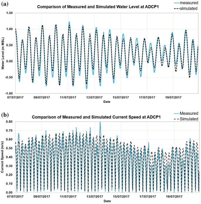
a Comparison of measured and simulated water level at ADCP1 and b comparison of measured and simulated current speed at ADCP1
-
(b)
Comparison of performance for different turbulence models
A typical 12-h time series of flood-ebb tidal cycles were extracted from the 2D far-field model and input as the velocity and tidal boundaries conditions for the 3D near-field CFD model. The 3D CFD model was setup to evaluate the performance of different turbulence models in predicting the water level and depth-averaged current speed at ADCP 2 and ADCP3. Three statistical indexes were used to compare the turbulence models (root mean square percentage error (RMSE), squared of Pearson product-moment correlation coefficient (R2) and mean absolute error (MAE)).

Figures 9 and 10 show the comparison of the simulated and measured water level at ADCP2 and ADCP3, respectively. The red line represents the linear trendline. The results show that there is a significant positive correlation between simulated and measured water level for all turbulence models with R2 of 0.99. RMSE for k–ε, k–ε RNG and k–ε turbulence models are 8.10% and 7.50% for ADCP2 and ADCP3, respectively. RMSE values for the LES model is slightly higher than other turbulence models, with 8.15% and 7.51% for ADCP2 and ADCP3, respectively. The LES model also reported highest MAE of 6.67 cm while the k–ε model has the lowest of 6.26 cm. In general, the simulated water level for all turbulence models are broadly consistent with the major trend of values within the k–ε model reported to have the best performance.

Comparison of the simulated and measured water level at ADCP2 for various turbulent models

Comparison of the simulated and measured water level at ADCP3 for various turbulent models
Figures 11 and 12 depict the comparison of the simulated and measured depth-averaged current speed at ADCP2 and ADCP3, respectively. Overall, good positive correlation is found between simulated and measured current speeds for all turbulence models. The average results of ADCP2 and ADCP3 show that the k–ε RNG model (with R2 of 0.76, RMSE of 10.31% and MAE of 5.06 cm/s) is a better predictor of current speed, compared with the other turbulence models. The analysis reveals that the LES model has slightly lower accuracy in predicting current speed around the existing intake structure. R2, RMSE and MAE for the LES model are reported as 0.75, 10.55% and 5.22 cm/s, respectively.

Comparison of the simulated and measured depth-averaged current speed at ADCP2 for various turbulent models

Comparison of the simulated and measured depth-averaged current speed at ADCP3 for various turbulent models
These comparisons reveal that the k–ε RNG model more accurately represents water level and current speed around an existing open offshore intake structure. Our findings support previous studies that indicated that the k–ε RNG model is more accurate when simulating low-intensity turbulence flows [18,19,20]. In contrast, the LES model has slightly lower accuracy in predicting water level and current speed. This may attribute to the fact that the LES model may require finer meshes and more computational efforts compared to the RANS based models. In the context of engineering application, computational cost and solution accuracy must be carefully balanced. With the same model meshes, k–ε RNG can provide good accuracy and reduce the computational costs compared with the LES model.
-
(c)
3D far-field model validation
The k–ε RNG model was selected to conduct the validation for the 3D near-field CFD model. 3D far-field model validation was carried out by comparing the simulated water level and depth-averaged current speed, throughout the continuous 8 days’ time series, with measured data at ADCP2, ADCP3 and ADCP4. Figures 13 and 14 show the comparison between the simulated and measured water level and current speed, respectively. The comparative results show that the simulated water level and current speed are in good agreement with the measured values. However, all current speed simulation results are slightly lower than the measured values. This may likely be attributed to the influence of wave action which was not considered in this study. RMSE values for water level and current speed at ADCP2, ADCP3 and ADCP4 are tabulated in Table 1. The RMSE value is less than 6% and 13% for water level and current speed respectively, which are acceptable for comparing the simulated data with the field measurements. Based on the 3D model validation, the k–ε RNG turbulence model was selected as the viscous model to simulate the flow kinematics around the open offshore intake structure.
Fig. 13 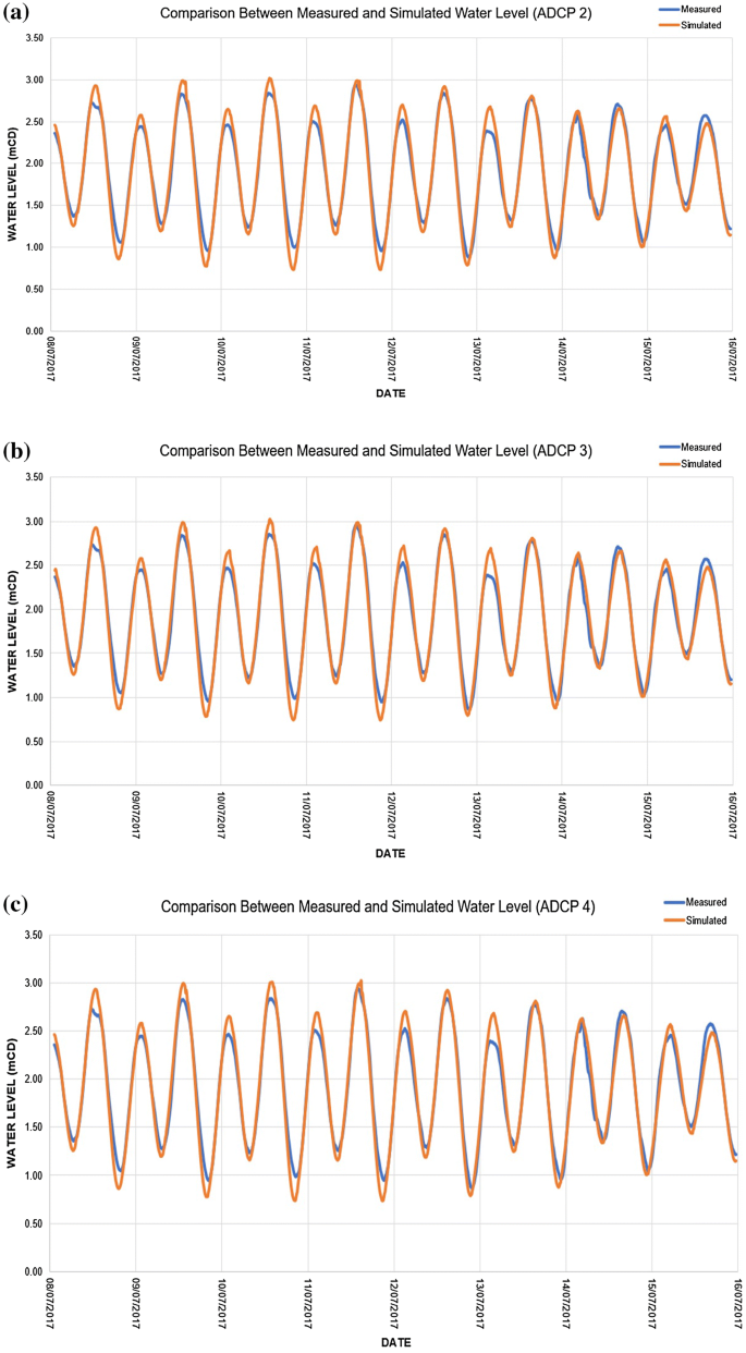
a Comparison between the measured and simulated water level at ADCP2, b comparison between the measured and simulated water level at ADCP3 and c comparison between the measured and simulated water level at ADCP4
Fig. 14 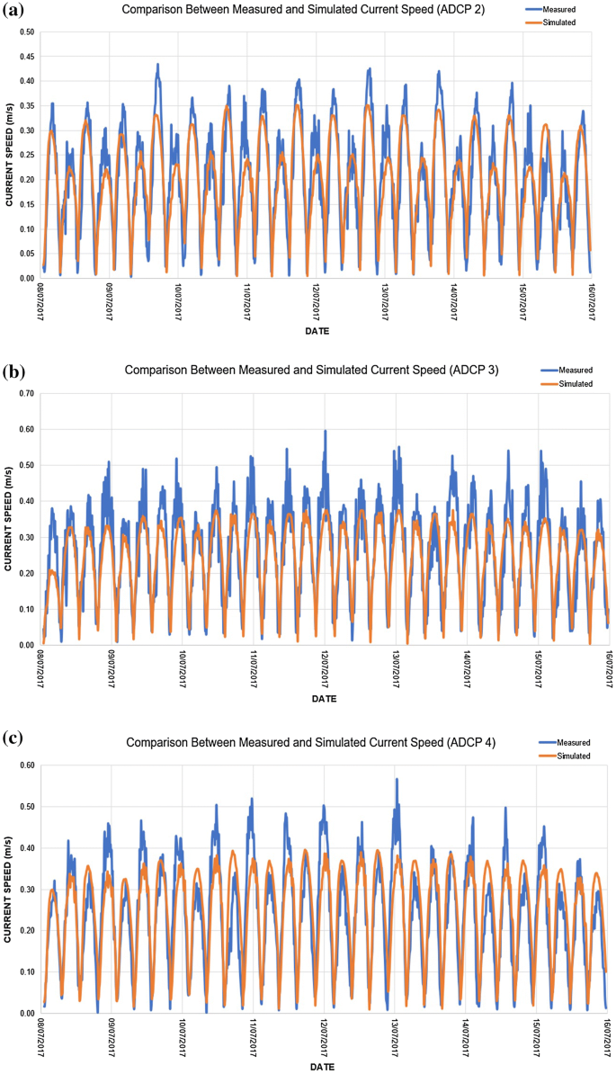
a Comparison between the measured and simulated current speed at ADCP2, b comparison between the measured and simulated current speed at ADCP3 and c comparison between the measured and simulated current speed at ADCP4
Table 1 RMSE values for water level and current speed for 3D model


4 Conclusion
A combined predictive modelling approach that couples the 2D far-field model and the 3D near-field CFD model was developed to compare the performance of different turbulence models in predicting the flow kinematics around an open offshore intake structure. It is important to compare the performance of various turbulence models to select an appropriate model for simulating the flow field around the open offshore intake. k–ε, k–ε RNG, k–ω and LES models have been used to model the water level and current speed around an existing intake structure. Our work has led us to conclude that:
-
The simulated water level for all turbulence models are broadly consistent with the major trend of measured values with k–ε model reported the best performance. The water level simulated by k–ε RNG model is also very close to the measurement values.
-
Comparison of the simulated current speed by the four turbulence models with the field measurement show that k–ε RNG model fits better than those predicted by the other models.
-
The analysis reveals that the LES model has slightly lower accuracy in predicting current speed around the existing intake structure. This may attribute to the fact that the LES model may require finer meshes and more computational efforts compared to the RANS based models.
-
With the same model meshes, the k–ε RNG model can provide good accuracy and reduce the computational costs compared to the LES model. This is very important in the context of engineering application where computational cost and solution accuracy must be carefully balanced.
-
Overall, the k–ε RNG model presents more accurately in predicting water level and current speed around an existing open offshore intake structure. Based on the 3D model validation, the k–ε RNG turbulence model was selected as the viscous model to simulate the flow kinematics around the open offshore intake structure.
References
Pankratz T (2015) Overview of intake systems for seawater reverse osmosis facilities. In: Missimer TM, Jones B, Maliva RG (eds) Intakes and outfalls for seawater reverse-osmosis desalination facilities: innovations and environmental impacts. Springer, New York, pp 3–17
Pita E, Sierra I (2011) Seawater intake structures. In: International symposium on outfall system, May 15–18, Mar del Plata, Argentina
Johnson PL (1988) Hydro-power intake design considerations. J Hydraul Eng 114(6):651–661
Khanarmuei MR, Rahimzadeh H, Kakuei AR, Sarkardeh H (2016) Effect of vortex formation on sediment transport at dual pipe intakes. Sadhana 41(9):1055–1061
Moghadam MK, Bajestan MS, Sedghi H (2010) Sediment entry investigation at the 30-degree water intake installed at trapezoidal channel. World Appl Sci J 11(1):82–88
Emamgholizadeh S, Torabi H (2008) Experimental investigation of the effects of submerged vanes for sediment diversion in the Veis (Ahwaz) Pump Station. J Appl Sci 8(13):2396–2403
Karami H, Farzin S, Sadrabadi MT, Moazeni H (2017) Simulation of flow pattern at rectangular lateral intake with different dike and submerged vane scenarios. J Water Sci Eng 10(3):246–255
Sefidkoohi RB, Shahidi A, Ramezani Y, Kahe M (2017) Simulation of flow pattern in intake by using a numerical model. Water Harvest Res 2(1):24–36
Tataroglu RM (2014) Numerical investigation of vortex formation at intake structures using Flow3D software. Master of Science in Civil Engineering, Middle East Technical University
Ruether N, Singh JM, Olsen NRB, Atkinson E (2005) 3D computation of sediment transport at water intakes. Proc Inst Civ Eng Water Manag 158:1–8
Yeganeh-Bakhtiary A, Zanganeh M, Kazemi E, Cheng L, Abd Wahab AK (2013) Euler–Lagrange two-phase model for simulating live-bed scour beneath marine pipelines. J Offshore Mech Arctic Eng 135:031705
Gonzalo D, Mariano DD, Alfredo L, Sergio OL (2012) Physical modeling and CFD comparison: case study of a hydo-combined power station in spillway mode. In: International junior researcher and engineer workshop on hydraulic structure
Cheng YL, Ying BF (2007) Numerical simulation and comparison of water intake-outlet methods in power plants. J Hydrodyn 19(5):623–629
Zhao LJ, Nohmi M (2012) Numerical simulation of free water surface in pump intake. IOP Conf Ser Earth Environ Sci 15:052035
Lucino C, Gonzalo Dur S (2010) Vortex detection in pump sumps by means of CFD. In: XXIV Latin American congress on hydraulics, Punta Del Este, Uruguay
Lu ZF, Yu L, Xu XY (2017) Comparative study on turbulence models simulating inorganic particle removal in a Pista grid chamber. J Environ Technol 14:1–12
Catalano P, Wang M, Iaccarino G, Moin P (2003) Numerical simulation of the flow around a circular cylinder at high Reynolds numbers. Int J Heat Fluid Flow 24:463–469
Sodja J (2007) Seminar on turbulence models in CFD. Doctoral dissertation, University of Ljubljana, Slovena
Kaheh M, Kashefipour SM, Dehghani A (2014) Comparison of k–ε and RNG k–ε turbulent models for estimation of velocity profiles along the hydraulic jump on corrugated beds. In: 6th International symposium on environmental hydraulics, LAHR. Athens, Greece
Yakhot V, Smith LM (1992) The renormalization group, the ε-expansion and derivation of turbulence models. J Sci Comput 7(1):35–61
Guimaraes F (2011) Research: anyone can do it. PediaPress, Mainz
Lesser GR, Roelvink JA, Van Kester JATM, Stelling GS (2004) Development and validation of a three-dimensional model. Coast Eng 51:883–915
Deltares (2014) Delft3D-FLOW user manual, 3.15.34158 ed. Deltares, Boussinesqweg
Egbert GD, Erofeeva SY (2002) Efficient inverse modelling of barotropic ocean tides. J Atmos Ocean Technol 19(2):183–204
Flow Science (2016) Flow3D v11.2 user’s manual. Flow Science Inc, SanataFe
Francis HH, Paul IN (1967) Turbulence transport equations. Phys Fluids 10(11):2323–2332
Yakhot V, Steven AO (1986) Renormalization group analysis of turbulence I: basic theory. J Sci Comput 1(1):3–51
Wilcox DC (2008) Formulation of the k–ω turbulence model revisited. AIAA J 46(11):2823–2838
Department of Irrigation and Drainage (DID) (2001) Guidelines for preparation of coastal engineering hydraulic study and impact evaluation: for hydraulic studies using numerical models. Kuala Lumpur, Malaysia, (45) dlm.PPS.14/2/23 Jld.2
Funding
This research was funded by Ministry of Education (MOE) Malaysia to Research Management Centre (RMC) of Universiti Teknologi Malaysia (UTM) under the Vote Number R.J130000.7809.4F979.
Author information
Authors and Affiliations
Corresponding author
Ethics declarations
Conflict of interest
The authors declare that they have no competing interests.
Additional information
Publisher's Note
Springer Nature remains neutral with regard to jurisdictional claims in published maps and institutional affiliations.
Rights and permissions
About this article

Cite this article
Lee, H.C., Wahab, A.K.A. Performance of different turbulence models in predicting flow kinematics around an open offshore intake. SN Appl. Sci. 1, 1266 (2019). https://doi.org/10.1007/s42452-019-1320-8
Received:
Accepted:
Published:
DOI: https://doi.org/10.1007/s42452-019-1320-8