Newton flows for elliptic functions II

Abstract

In our previous paper we associated to each non-constant elliptic function f on a torus T a dynamical system, the elliptic Newton flow corresponding to f. We characterized the functions for which these flows are structurally stable and showed a genericity result. In the present paper we focus on the classification and representation of these structurally stable flows. The phase portrait of a structurally stable elliptic Newton flow generates a connected, cellularly embedded graph $\mathscr {G}(f)$ on a torus T with r vertices, 2r edges and r faces that fulfil certain combinatorial properties (Euler, Hall) on some of its subgraphs. The graph $\mathscr {G}(f)$ determines the conjugacy class of the flow [classification]. A connected, cellularly embedded toroidal graph $\mathscr {G}$ with the above Euler and Hall properties, is called a Newton graph. Any Newton graph $\mathscr {G}$ can be realized as the graph $\mathscr {G}(f)$ of the structurally stable Newton flow for some function f. This leads to: up till conjugacy between flows and (topological) equivalency between graphs, there is a one to one correspondence between the structurally stable Newton flows and Newton graphs, both with respect to the same order r of the underlying functions f [representation]. Finally, we clarify the analogy between rational and elliptic Newton flows, and show that the detection of elliptic Newton flows is possible in polynomial time. The proofs of the above results rely on Peixoto’s characterization/classification theorems for structurally stable dynamical systems on compact 2-dimensional manifolds, Stiemke’s theorem of the alternatives, Hall’s theorem of distinct representatives, the Heffter–Edmonds–Ringer rotation principle for embedded graphs, an existence theorem on gradient dynamical systems by Smale, and an interpretation of Newton flows as steady streams.

1 Elliptic Newton flows: a recapitulation

In order to clarify the context of the present paper, we recapitulate some earlier results.

1.1 Elliptic Newton flows on the plane and on a torus

Let f be an elliptic (i.e., meromorphic, doubly periodic) function of order on the complex plane $\mathbb {C}$ with $(\omega _{1}, \omega _{2})$, $\mathrm{Im}\,{\omega _{2}}/{\omega _{1}} >0$, as basic periods spanning a lattice ${\Lambda }$ .

The planar elliptic Newton flow $\overline{\mathscr {N} }(f)$ is a $C^{1}$-vector field on $\mathbb {C}$, defined as a desingularized version ¹ of the planar dynamical system, $\mathscr {N}(f)$, given by (cf. [8])

(1)

On a non-singular, oriented $\overline{\mathscr {N} }(f)$-trajectory z(t) we have (cf. [8]):

• $\mathrm{arg}\,f =\mathrm{constant}$ and |f(z(t))| is a strictly decreasing function on t.

So that an $\overline{\mathscr {N} }(f)$-equilibrium is:

• attractor, or repellor, or saddle; see the comments on Fig. 1, where N(f), P(f) and C(f) stand for, respectively, the set of zeros, poles and critical points for f.

Fig. 1

Local phase portraits around equilibria of $\overline{\mathscr {N}}(f)$

Comments on Fig. 1:

Figure 1 (a), (b): In a k-fold zero (pole) for f the flow $\overline{\mathscr {N} }(f)$ exhibits a stable (unstable) star node and each (principal) value of $\mathrm{arg}\,f$ appears precisely k times on equally distributed incoming (outgoing) trajectories. Moreover, two different incoming (outgoing) trajectories intersect under a non-vanishing angle ${{\Delta }}/{k}$, where ${\Delta }$ stands for the difference of the $\mathrm{arg}\,f$-values on these trajectories.

Figure 1 (c), (d): In case of a k-fold critical point (i.e. a k-fold zero for , no zero for f) the flow $\overline{\mathscr {N} }(f)$ exhibits a k-fold saddle, the stable (unstable) separatrices being equally distributed around this point. The two unstable (stable) separatrices at a onefold saddle, see Fig. 1 (c), constitute the “local” unstable (stable) manifold at this saddle point.

Functions of the type f correspond to the meromorphic functions on the complex torus $T({\Lambda })$ (). So, we can interpret $\overline{\mathscr {N} }(f)$ as a global $C^{1}$-vector field, denoted² $\overline{\overline{\mathscr {N}} }(f)$, on the Riemann surface $T({\Lambda })$ and it is allowed to apply results for $C^{1}$-vector fields on compact differential manifolds, such as certain theorems of Poincaré–Bendixon–Schwartz on limiting sets and those of Baggis–Peixoto on $C^{1}$-structural stability. In particular, the local phase portraits around $\overline{\overline{\mathscr {N}} }(f)$-equilibria are as in Fig. 1.

1.2 The canonical form for a toroidal Newton flow; the topology $\tau _{0}$

It is well known that the function f has precisely r zeros and r poles (counted by multiplicity) on the half open / half closed period parallelogram given by .

Denoting these zeros and poles by $a_{1},\ldots ,a_{r}$, respectively $b_{1}, \ldots ,b_{r}$, we have (cf. [8, 16]):

(2)

and thus

(3)

where and are the zeros, respectively poles, for f on $T({\Lambda })$ and stands for the congruency class $\mathrm {mod}\, {\Lambda }$ of a number in $\mathbb {C}$.

Theorem 1.1

(Canonical form for toroidal Newton flows)

• Given a flow $\overline{\overline{\mathscr {N}} }(f)$ on $T({\Lambda })$, there exists an elliptic function $f^{*}$ of order r with period lattice together with a homeomorphism 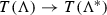mapping the phase portraits of $\overline{\overline{\mathscr {N}} }(f)$ and $\overline{\overline{\mathscr {N}} }(f^{*})$ onto each other, thereby respecting the orientations of the trajectories.

• Moreover: If $a^{*}_{1}, \ldots ,a^{*}_{r}$, respectively $b^{*}_{1}, \ldots ,b^{*}_{r}$, are the zeros and poles of $f^{*}$ in $P^{*}$ , then

  

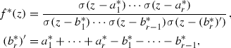
  where $\sigma$ stands for the Weierstrass’ sigma function w.r.t. the lattice .

• Conversely: if $c_{1}, \ldots ,c_{r}$, respectively $d_{1}, \ldots ,d_{r}$, stand for any pair of r tuples in $P^{*}$ that fulfil relations (2), then due to the basic properties of the quasi periodic function $\sigma$, a function of the form

  

  with $d_{r}' = c_{1}+ \cdots +c_{r} - d_{1}- \cdots -d_{r-1}$, is elliptic w.r.t. to with , respectively , as zeros, poles on .

Now, it is not difficult to see that the elliptic functions of order r, and also the underlying toroidal Newton flows, can be represented by the set of all ordered pairs

of congruency classes with , $i=1, \ldots , r$, that fulfil (3). This representation space can be endowed with a topology, say $\tau _{0}$, that is induced by the Euclidean topology on $\mathbb {C}$, and is natural in the following sense (cf. [8]): given an elliptic function f of order r and $\varepsilon >0$ sufficiently small, there exists a $\tau _{0}$-neighbourhood $\mathscr {O}$ of f such that for any $g \in \mathscr {O}$, the zeros (poles) for g are contained in $\varepsilon$-neighbourhoods of the zeros (poles) for f.

1.3 Structural stability

Let $E_{r}({\Lambda })$ be the set of all elliptic functions f of order r on the torus and $N_{r}({\Lambda })$ the set of all toroidal Newton flows $\overline{\overline{\mathscr {N}} }(f)$. We assume (no loss of generality; see Sect. 1.2) that ${\Lambda }={\Lambda }_{1, i}$, and write $E_{r}({\Lambda })=E_{r}$, $T({\Lambda })=T$ and $N_{r}({\Lambda })=N_{r}$.

By X(T) we mean the set of all $C^{1}$-vector fields on T, endowed with the $C^{1}$-topology. The topology $\tau _{0}$ on $E_{r}$ and the $C^{1}$-topology on X(T) are matched by (cf. [8]):

Lemma 1.2

The map $E_{r} \rightarrow X(T):f \mapsto \overline{\overline{\mathscr {N}}} (f)$ is $\tau _{0}$-$C^{1}$-continuous.

Two flows $\overline{\overline{\mathscr {N}} }(f)$ and $\overline{\overline{\mathscr {N}} }(g)$ in $N_{r}$ are called conjugate, denoted $\overline{\overline{\mathscr {N}}} (f) \sim \overline{\overline{\mathscr {N}}} (g)$, if there is a homeomorphism from T onto itself mapping maximal trajectories of $\overline{\overline{\mathscr {N}} }(f)$ onto those of $\overline{\overline{\mathscr {N}} }(g)$, thereby respecting the orientations of these trajectories.

We call the flow $\overline{\overline{\mathscr {N}}} (f)$ $\tau _{0}$-structurally stable, if there is a $\tau _{0}$-neighborhood $\mathscr {O}$ of f such that for all $g \in \mathscr {O}$ we have $\overline{\overline{\mathscr {N}}} (f) \sim \overline{\overline{\mathscr {N}}} (g)$. The set of all structurally stable Newton flows $\overline{\overline{\mathscr {N}}} (f)$ is denoted by .

By Lemma 1.2, it follows that $C^{1}$-structural stability for $\overline{\overline{\mathscr {N}}} (f)$ implies $\tau _{0}$-structural stability for $\overline{\overline{\mathscr {N}}} (f)$. So, when discussing structural stable toroidal Newton flows we will skip the adjectives $\tau _{0}$ and . We proved (cf. [8]):

Theorem 1.3

(Characterization and genericity of structural stability)

• (I) if and only if the function f is non-degenerate, i.e., all zeros, poles and critical points for f are simple, and no critical points for f are connected by $\overline{\overline{\mathscr {N}}} (f)$-trajectories.

• (II) The set of all non-degenerate functions of order r is open and dense in $E_{r}$.

Fig. 2

Basin of repulsion (attraction) in the phase portrait of $\overline{\overline{\mathscr {N}}} (f)$ for a pole (zero) of f

We list some properties that will play a role in the sequel, see the comments on Fig. 1:

Lemma 1.4

(Properties of structurally stable toroidal Newton flows $\overline{\overline{\mathscr {N}}} (f)$)

• (a) If $\overline{\overline{\mathscr {N}}} (f)$ is structurally stable, then also $\overline{\overline{\mathscr {N}}} ({1}/{f})$ is, and . [Duality]

• (b) There are precisely 2r orthogonal saddles for $\overline{\overline{\mathscr {N}}} (f)$.

• (c) The boundary of the basin of a repellor (attractor) is made up by the unstable (stable) manifolds at the saddles situated in this boundary (cf. Fig. 2).

As an illustration we present in Figs. 3 and 4 planar/toroidal Newton flows for Jacobian functions $\mathrm{sn}_{\omega _{1}, \omega _{2}}$ with only simple attractors, repellors and saddles; see also [1, 8] and the forthcoming Remark 2.15. For more examples of (structurally stable) Newton flows, see [9].

Fig. 3

Planar and toroidal Newton flows for $\mathrm{sn}_{\omega _{1},\omega _{2}}$; structurally stable

Fig. 4

Planar Newton flow for $\mathrm{sn}_{\omega _{1},\omega _{2}}$; not structurally stable

1.4 Toroidal versus rational Newton flows; purpose of the paper

If we choose for f rational functions (meromorphic on the Riemann sphere $S^{2}$), we obtain the class of so-called spherical Newton flows. These flows have many concepts/features in common with (the class of) toroidal Newton flows and are already studied before (cf. [10,11,12,13]); in fact, characterization and genericity results, analogous to Theorem 1.3, have been proved. Moreover, spherical Newton flows can be classified and represented in terms of certain sphere graphs (i.e. the “principal parts” of the phase portraits of structurally stable spherical Newton flows). The target of the present paper is to prove such a classification and representation result for toroidal Newton flows.

2 Structurally stable elliptic Newton flows: classification

In this section, let f be non-degenerate of order r, thus $\overline{\overline{\mathscr {N}}} (f)$ is structurally stable. Then, the following definition makes sense: (cf. Sect. 1.1, Lemma 1.4).

Definition 2.1

The graph $\mathscr {G}(f )$, , on the torus T is given by:

• Vertices are the r zeros for f on T (as attractors for $\overline{\overline{\mathscr {N}} }(f)$).

• Edges are the 2r unstable manifolds at the critical points for f on T as $\overline{\overline{\mathscr {N}} }(f)$-saddles.

Note that the faces of $\mathscr {G}(f )$ are precisely the r basins of repulsion of the poles, say , $j=1, \ldots , r$, for f on T (as repellors for $\overline{\overline{\mathscr {N}} }(f)$) and will be denoted by ; their boundaries by . These boundaries, consisting of unstable manifolds at saddles for $\overline{\overline{\mathscr {N}} }(f)$, are subgraphs of $\mathscr {G}(f )$, see Fig. 2.

Analogously, we define the graph,³ say $\mathscr {G}^{*}(f )$, on the poles and the stable $\overline{\overline{\mathscr {N}} }(f)$-manifolds at the critical points for f on T.

Lemma 2.2

Both $\mathscr {G}(f )$ and $\mathscr {G}^{*}(f )$ are multigraphs⁴ embedded in T.

Proof

If $\mathscr {G}(f )$ would have a loop, the two unstable $\overline{\overline{\mathscr {N}} }(f)$-separatrices at some critical point for f would approach the same zero, say , on T. In that case, the zeros (simple!) for f in the plane, corresponding to , will be approached by two different trajectories (of the planar version $\overline{\mathscr {N}}(f)$) with the same value of $\mathrm{arg}\,f$. This is impossible (cf. the comments on Fig. 1). The second part of the assertion follows by interchanging the roles of the poles and zeros for f. $\square$

Corollary 2.3

An edge in $\mathscr {G}(f )$ or $\mathscr {G}^{*}(f )$ is contained in the boundaries of two different faces.

Next we introduce a graph on T, denoted , which may be considered as the “common refinement of $\mathscr {G}(f)$ and $\mathscr {G}^{*}(f )$”.

Definition 2.4

The vertices of are defined as the zeros, poles and critical points for f, whereas the edges are the stable and unstable separatrices of $\overline{\overline{\mathscr {N}} }(f)$ at the critical points for f.

The faces of are the so-called canonical regions for $\overline{\overline{\mathscr {N}} }(f)$, i.e. the connected components of what is left after deleting from T all the $\overline{\overline{\mathscr {N}} }(f)$-equilibria and all stable and unstable manifolds at the saddles of $\overline{\overline{\mathscr {N}} }(f)$. A priori, the canonical regions of a $C^{1}$-structurally stable flow on T (without closed orbits) are of one of the Types 1, 2, 3 in Fig. 5 (cf. Fig. 2, [20]). However, by Lemma 2.2 the flow $\overline{\overline{\mathscr {N}} }(f)$—although structurally stable—cannot admit canonical regions of Types 2 and 3.

Fig. 5

The canonical regions of a structural stable flow on T

So, we only have to deal with canonical regions of Type 1. Since all zeros, poles and critical points for f are simple, we find (see Sect. 1.1):

Lemma 2.5

In a canonical region of $\overline{\overline{\mathscr {N}} }(f)$, the angles (anti-clockwise measured) at the pole and the zero are well defined, strictly positive and equal.

Since a face is built up from all canonical regions that have in common, we find:

Corollary 2.6

All (anti-clockwise measured) angles spanning a sector of at the vertices in its boundary, are non-vanishing and sum up to $2 \pi$.

Lemma 2.7

Each subgraph is Eulerian.⁵

Proof

Traverse the set of all canonical regions centered at once. In this way we determine a closed walk, say , through all the vertices and edges of ; see Fig. 6. By Corollary 2.3, this walk contains each edge of only once (since otherwise the two stable separatrices at the saddle on such an edge must originate from ). So, is the desired Euler trail. $\square$

The walk in the above proof will be referred to as to the facial walk for . Analogously, we define the (Eulerian!) facial walks on the boundaries of the $\mathscr {G}^{*}(f )$-faces (i.e., the basins of attraction of the zeros, say , $i=1, \ldots , r$, for f on T as attractors for the Newton flow $\overline{\overline{\mathscr {N}} }(f)$).

Fig. 6

Oriented facial walks on $\mathscr {G}(f )$ and $\mathscr {G}^{*}(f )$

Remark 2.8

Note that in these facial walks the same vertex may occur more than once. However, by Lemma 2.2, a vertex in a facial walk cannot be adjacent to itself.

We endow (the faces of) $\mathscr {G}(f )$ with a coherent orientation as follows: for each facial walk we demand that the (constant) values of $\mathrm{arg}\,f(z)$ on consecutive edges form an increasing sequence. This is imposed by the anti-clockwise ordering of the $\mathscr {G}(f )$-edges around a common vertex, which on its turn induces clockwise orientations of the $\mathscr {G}^{*}(f )$-edges incident to a given vertex. This leads to an orientation of (the facial walks on) $\mathscr {G}^{*}(f )$ which is opposite to the orientation of $\mathscr {G}(f )$ as chosen before; see Fig. 6. From now on we assume that all graphs $\mathscr {G}(f )$ and $\mathscr {G}^{*}(f )$, , are oriented in this way: $\mathscr {G}(f )$ always clockwise; $\mathscr {G}^{*}(f )$ always anti-clockwise. By we mean $\mathscr {G}(f )$ with anti-clockwise orientation and by the clockwise oriented graph $\mathscr {G}^{*}(f )$.

Lemma 2.9

The (multi)graphs $\mathscr {G}(f )$ and $\mathscr {G}^{*}(f )$ are connected and cellularly embedded.⁶

Proof

We focus on $\mathscr {G}(f )$ and follow the treatise [18] closely. Consider the r facial walks and put length . Consider for each a so-called facial polygon, i.e. a polygon in the plane with sides labelled by the edges of (taking the orientation of into account), so that each polygon is disjoint from the other polygons. Now we take all facial polygons. Each $\mathscr {G}(f )$-edge occurs precisely once in two different facial walks and this determines orientations of the sides of the polygons. By identifying each side with its mate, we construct (cf. [18]) an orientable, connected surface S, homeomorphic to T, and (in S) a 2-cell embedded graph, which is—up to an isomorphism—equal to $\mathscr {G}(f )$. By Euler’s formula for graphs on T (cf. [5]), $\mathscr {G}(f )$ is connected and orientable as well. Finally, we note that a 2-cell embedding is always cellular (cf. [18]). $\square$

The abstract directed graph, underlying , will be denoted by $\mathbb {P}(f )$, where the directions are induced by the orientations of the (un)stable separatrices at $\overline{\overline{\mathscr {N}} }(f)$-saddles. Each canonical region is represented by a quadruple of directed edges in $\mathbb {P}(f )$, and is associated with precisely one pole, one zero (in opposite position) and two critical points for f on T. Following Peixoto [19, 20], such a quadruple is called a distinguished set (of Type 1). The graph $\mathbb {P}(f )$ together with the collection of all distinguished sets is denoted by . We say “ is realized by the distinguished graph of $\overline{\overline{\mathscr {N}} }(f)$ on T”.

We need a classical result due to Peixoto (cf. [20]) on structurally, $C^{1}$-stable vector fields on 2-dimensional compact manifolds. In the context of our elliptic Newton flows this yields (together with Lemma 1.2): if , then

(4)

Here, $\sim$ in the l.h.s stands for “conjugacy” and $\sim$ in the r.h.s. for isomorphism between and (as directed abstract graphs), preserving the distinguished sets and respecting the cyclic ordering (induced by the embedding in T) of the distinguished sets around a common vertex.

Theorem 2.10

(Classification of structurally stable elliptic Newton flows by graphs) Let $\overline{\overline{\mathscr {N}} }(f)$ and $\overline{\overline{\mathscr {N}} }(h)$ be structurally stable (thus ), then

$$\begin{aligned} \overline{\overline{\mathscr {N}} }(f) \sim \overline{\overline{\mathscr {N}} }(h) \quad \Longleftrightarrow \quad \mathscr {G}(f) \sim \mathscr {G}(h) \;\;(\text {and thus also } \mathscr {G}^{*}(f) \sim \mathscr {G}^{*}(h)), \end{aligned}$$

where $\sim$ in the r.h.s. stands for equivalency between the oriented graphs (i.e., an isomorphism respecting their orientations).

Proof

Apply (4) to $\overline{\overline{\mathscr {N}} }(f)$ and $\overline{\overline{\mathscr {N}} }(h)$. $\square$

The graph $\mathscr {G}({1}/{f})$ is also well defined (with as faces $F_{a_{i}}({1}/{f})$) and associated with the structurally stable flow . The flow $\overline{\overline{\mathscr {N}} }({1}/{f})$ is the dual version of $\overline{\overline{\mathscr {N}} }(f)$, i.e., $\overline{\overline{\mathscr {N}} }({1}/{f})$ is obtained from $\overline{\overline{\mathscr {N}} }(f)$ by reversing the orientations of the trajectories of the latter flow, thereby changing repellors into attractors and vice versa. Clearly, $\mathscr {G}({1}/{f})$ and $\mathscr {G}^{*}(f)$ coincide, be it with opposite orientations, i.e., , where, due to our convention on orientations, $\mathscr {G}({1}/{f})$ is clockwise oriented. Also, we have .

Note that, in general, $\overline{\overline{\mathscr {N}} }(f)$ and $\overline{\overline{\mathscr {N}} }({1}/{f})$ are not conjugate. In the special case where $\overline{\overline{\mathscr {N}} }(f) \sim \overline{\overline{\mathscr {N}} }({1}/{f})$ we call these flows self-dual, and we have (Theorem 2.10)

If holds, we call $\mathscr {G}(f)$ and $\mathscr {G}^*(f)$ self-dual.

Remark 2.11

(On the classification under conjugacy and duality) Conjugate flows are considered as equal. Although, in general, $\overline{\overline{\mathscr {N}} }(f)$ and $\overline{\overline{\mathscr {N}} }({1}/{f})$ are not conjugate, it is reasonable to consider also these flows, being related by a trivial (but orientation reversing) identity, as “equal”. See our paper [9].

Remark 2.12

(On self-duality) If $\overline{\overline{\mathscr {N}} }(f)$ is self-dual and conjugate with $\overline{\overline{\mathscr {N}} }(h)$, then $\overline{\overline{\mathscr {N}} }(h)$ is also self-dual.

Corollary 2.13

Any two structurally stable 2nd order elliptic Newton flows are conjugate. In particular, these flows are self-dual.

Proof

Let $\overline{\overline{\mathscr {N}} }(f)$, $f \in \widetilde{E}_{2}$, be chosen arbitrarily. By Corollary 2.3, the two faces of $\mathscr {G}(f)$ share their boundaries. So, the common facial walk of these faces is built up from the four $\mathscr {G}(f)$-edges and the two $\mathscr {G}(f)$-vertices (each appearing twice but not consecutive!). Hence, compare the construction in the proof of Lemma 2.9 and see Fig. 7, $\mathscr {G}(f)$ is determined by the anti-clockwise oriented walk . The same holds for any other flow $\overline{\overline{\mathscr {N}} }(h)$ with facial walk $w_{h}$, $h \in \widetilde{E}_{2}$. Apparently, and $w_{h}$ maybe considered as equal, under a suitably chosen relabeling of their vertices and edges. Hence $\mathscr {G}(f) \sim \mathscr {G}(h)$ and thus $\overline{\overline{\mathscr {N}} }(f) \sim \overline{\overline{\mathscr {N}} }(h)$. In particular, put $h={1}/{f}$, then we find $\mathscr {G}(f) \sim \mathscr {G}({1}/{f})$, compare Fig. 7 and Remark 2.12.$\square$

Remark 2.14

For basically the same proof of Corollary 2.13, see [22].

Remark 2.15

The flow $\overline{\overline{\mathscr {N}} }$(sn), in the non-rectangular case (cf. Fig. 3) exhibits an example of a 2nd order structurally stable elliptic Newton flow. By Corollary 2.13, this is the only possibility (up to conjugacy) for a flow in $\widetilde{N}_{2}$. Note that the flow in Fig. 4 (rectangular case) is not structurally stable (because of the saddle connections).

We proceed by introducing flows that are closely related to $\mathscr {N}(f),\overline{\mathscr {N} }(f)$ and $\overline{\overline{\mathscr {N}} }(f)$: the so-called rotated Newton flows.

Fig. 7

The graphs $\mathscr {G}(f)$ and $\mathscr {G}^{*}(f)$, $f\in \widetilde{E}_{2}$

Definition 2.16

For $f \in E_{r}$, let be a dynamical system of the type

Apparently, is a complex analytic vector field outside the set C(f) of critical points for f. As in Sect. 1.1, we turn into a $C^{1}$-system on the whole plane with (on $\mathbb {C} \backslash C(f)$) the same phase portrait as by . The function f, being elliptic, the system can be interpreted as a $C^{1}$-flow on T and as such it will be referred to as to , in particular,

Lemma 2.17

Let be the (maximal) -trajectory through a non-equilibrium , then:

• (i) .

• (ii) A zero or pole for f is a center for .

• (iii) A k-fold critical point for f is a k-fold saddle for .

Proof

Assertions (i) and (iii): use . Note that outside $N(f) \cup P(f)$ the flow can be considered as the Newton flow for .

For assertion (ii): let $z_{0}$ be a zero or pole for f with multiplicity k, thus an isolated zero for . In a neighborhood of $z_{0}$, system is linearly approximated by

Thus $z_{0}$ is a non-degenerate equilibrium for with characteristic roots . By the first assertion in the lemma, a regular integral curve through a point $\check{z}$ close to $z_{0}$, but $\ne z_{0}$, cannot end up at or leave from $z_{0}$. Hence, this point is neither a focus, nor a centro-focus for (cf. [2]) and must be a center for . $\square$

In view of the above assertion (i), a closed orbit for cannot be a limit cycle, and (by (ii)) a separatrix leaving a saddle $\sigma _{1}$ must approach a saddle $\sigma _{2}$. Moreover, this separatrix cannot connect $\sigma _{1}$ to itself, i.e. $\sigma _{1} \ne \sigma _{2}$. In fact, let $\sigma _{1}=\sigma _{2}$, since there holds that ,

which is impossible, see Fig. 8 and the comments on Fig. 1.

Fig. 8

No “self-connected” -saddles; $\sigma _{1}$ is twofold;

Note that—when introducing rotated Newton flows—no additional restrictions were laid upon the function f. But now, we return to the case of non-degenerate functions f. Then has 2r simple saddles (corresponding to the critical points for f) with altogether 4r separatrices, connecting different saddles. So, we may introduce:

Definition 2.18

The graph , $f \in \check{E}_{r}$, on the torus T is given by:

• Vertices are the 2r critical points for f (as saddles for ) on T.

• Edges are the 4r separatrices at the critical points for f (as -saddles) on T.

Since all zeros and poles for f are centers for , each -face contains only one zero or one pole for f. Moreover, the graph is cellularly embedded. Hence, the graph has 2r faces.

Lemma 2.19

Let c be an arbitrary, strictly positive real number and put . Then there holds:

• (i) The level set $L_{c}$ is a regular curve in $\mathbb {R}^{2}$ (i.e., $\mathrm{grad}\,|f(z)| \ne 0$ for all $z \in L_{c}$) if and only if $L_{c}$ contains no critical points for f.

• (ii) The graph , $f \in \check{E}_{r}$, is connected. In particular, f(z) admits the same absolute value at all critical points z.

Proof

(i) Use the Cauchy–Riemann equations. (ii) Apply Euler’s formula for toroidal graphs (cf. [5]). $\square$

We orient the edges of according to their orientation as -trajectories. Let $A_{i}$ and be open subsets of $\mathbb {C}$, corresponding to the (open) faces of that are determined by the zero $a_{i}$, respectively the pole , for f. Hence, the boundaries of $A_{i}$ are clockwise oriented, but those of anti-clockwise. Since we have: reversing the orientations in turns this graph into and thus, by Lemma 2.19 (ii), $|f(z)|=1$ on . See Fig. 9 for (parts of) the graphs and . A canonical $\overline{\overline{\mathscr {N}} }(f)$-region, with in opposite position, and the saddles $\sigma , \sigma '$ consecutive w.r.t. the orientation of $A_{i}$ (or ), will be denoted by $R_{ij}(\sigma , \sigma ')$ and it is contained in . Note that, in general, this intersection contains more canonical regions of type . But even so, these regions are separated by canonical regions, not of this type; compare Remark 2.8. In view of Sect. 1.1 and Lemma 2.17 (i), under f the net of $\overline{\overline{\mathscr {N}}}(f)$- and -trajectories on $R_{ij}(\sigma , \sigma ')$ is homeomorphically mapped onto a polar net in a sector of the -plane ($u=\mathrm{Re}\,f$, $v=\mathrm{Im}\,f$), namely

Analogously, 1 / f maps the net of $\overline{\overline{\mathscr {N}}}(f)$- and -trajectories on $R_{ji}(\sigma , \sigma ')$ onto a polar net in a sector of the -plane ($U=\mathrm{Re}\,{1}/{f}$, $V=\mathrm{Im}\,{1}/{f}$), namely

So, the polar nets on $s_{ij}(\sigma , \sigma ')$ and $S_{ij}(\sigma , \sigma ')$ correspond under the inversion⁷

Fig. 9

The graphs and for f and 1 / f in $\widetilde{E}_{r}$

Next we turn to the relationship between Newton flows and steady streams.

Remark 2.20

(Newton flows as steady streams) For $f \in \check{E}_{r}$, we consider the planar steady stream [15] with complex potential $w(z)=-\log f(z)$, potential function ${\Phi }(x,y)=-\log |f(z)|$ and stream function , where $x=\mathrm{Re}\,z$, $y=\mathrm{Im}\,z$. Then the equipotential lines are given by $- \log |f(z)|=$ constant, the stream lines by and the velocity field by the complex conjugate of $w'(z)$, i.e.

Moreover, the zeros (poles) for f are just the sinks (sources) of strength 1, whereas the critical points for f are the onefold stagnation points of the stream, compare also [8]. So, the “orthogonal net of the stream- and equipotential-lines” of the planar steady stream is a combination of the phase portraits of $\overline{\mathscr {N} }(f)$ and , see Fig. 10.

Fig. 10

The steady stream $w(z)=-\log f(z)$, $f \in \check{E}_{r}$

Hence we may interpret the pair () as a toroidal desingularized version of our planar steady stream.

Finally, we clarify the “steady stream character” of the structurally stable elliptic Newton flows from the point of view of the Riemann surface T.

Firstly, we note that the polar net on open (!) sectors as $s_{ij}(\sigma , \sigma ')$ and $S_{ij}(\sigma , \sigma ')$ is just the stream and equipotential lines of the steady stream with complex potential , respectively . In particular, these stream and equipotential lines exhibit the phase portraits of respectively the flows , , and , on $s_{ij}(\sigma , \sigma ')$ and $S_{ij}(\sigma , \sigma ')$ respectively. Deleting from T all zeros, poles and critical points for f, we obtain “the reduced torus” $\check{T}$, an open submanifold of T.

Now the collection

exhibits a covering of $\check{T}$ with open neighborhoods. Apparently, only in the case of pairs a non-empty intersection is possible. Even so, the intersection

consists of the disjoint union of sets of the type , say $R_{ij}^{1}, \ldots ,R_{ij}^{s}$. (Note that occurs in as many times as occurs in $w_{a_{i}}$.) This turns our covering into an atlas for $\check{T}$ with smooth (even complex analytic) coordinate transformations, induced by the inversion $u+iv \leftrightarrow 1/(u+iv)=U+iV$. With aid of this atlas, we may interpret $\overline{\overline{\mathscr {N}} }(f)$ and on each canonical region as the pull back of the most simple⁸ planar flows , and on the various sectors and respectively. Glueing the canonical regions along the $\overline{\overline{\mathscr {N}} }(f)$-trajectories in their common boundaries, we obtain the restrictions to $\check{T}$ of our original (rotated) Newton flows. In particular, the flows and lead to an analytic function on $\check{T}$, namely the restriction , with as isolated singularities the zeros, poles and critical points for f. By continuous extension to this singularities, we find the original flows $\overline{\overline{\mathscr {N}} }(f)$ and . For an illustration, see Figs. 11 and 12.

Fig. 11

The canonical regions $R_{ij}$, and the sectors $s_{ij}(\sigma , \sigma ')$ and $S_{ij}(\sigma , \sigma ')$

Fig. 12

and its images under f and 1 / f ($s=3$)

3 Newton graphs

Throughout this section, the connected graph $\mathscr {G}$ is a cellular embedding in T, seen as a compact, orientable, Hausdorff topological space of an abstract connected multigraph G (i.e., no loops) with r vertices, 2r edges ($r \geqslant 2$); $r=\mathrm{order}\,\mathscr {G}$.

The forthcoming analysis strongly relies on some concepts from classical graph theory on surfaces, which—in order to fix terminology—will be briefly reviewed.⁹

3.1 Cellularity; geometric duals

Since $\mathscr {G}$ is cellularly embedded, we may consider (cf. [18]) the rotation system ${\Pi }$ for $\mathscr {G}$:

where the local rotation $\pi _{v}$ at v is the cyclic permutation of the edges incident with v such that $\pi _{v}(e)$ is the successor of e in the anti-clockwise ordering around v.

If stands for an edge, with end vertices $v'$ and , we define a ${\Pi }$-walk (facial walk¹⁰), say w, on $\mathscr {G}$ as follows:

The face traversal procedure: Consider an edge $e_{1}=(v_{1}v_{2})$ and the closed walk¹¹ $w=v_{1}e_{1}v_{2}e_{2}v_{3} \ldots v_{k}e_{k}v_{1}$, which is determined by the requirement that, for $i=1, \ldots , \ell$, we have $\pi _{v_{i+1}}(e_{i})=e_{i+1}$, where $e_{\ell +1}=e_{1}$ and $\ell$ is minimal.

Apparently, such “minimal” $\ell$ exists since $\mathbf{G}$ is finite. Note that each edge occurs either once in two different ${\Pi }$-walks, or twice (with opposites orientations) in only one ${\Pi }$-walk; in particular, the first edge in the same direction which is repeated when traversing w, is $e_{1}$. As in the proof of Lemma 2.9, these ${\Pi }$-walks can be used to construct (patching the facial polygons along identically labelled sides) a surface S and in S a so-called 24-cell embedded graph with faces determined by the facial polygons. By Euler’s formula (cf. [5]), there are r facial walks. So, S is homeomorphic to T and the 2-cell embedded graph is isomorphic to $\mathscr {G}$. By the Heffter–Edmonds–Ringel rotation principle, the graph $\mathscr {G}$ is uniquely determined up to isomorphism by its rotation system. We say $\mathscr {G}$ is generated by ${\Pi }$.

From now on, we suppress the role of the underlying abstract graph $\mathbf{G}$ and will not distinguish between the vertices of $\mathscr {G}$ and those of $\mathbf{G}$. Occasionally, $\mathscr {G}$ will be referred to as to the pair ($\mathscr {G}, {\Pi }$). The $\mathscr {G}$-faces (as well as the corresponding facial polygons) are denoted by ; their boundaries (as well as the corresponding ${\Pi }$-walks) by , $j=1, \ldots ,r$. We denote the sets of all vertices, edges and faces of $\mathscr {G}$ by $V(\mathscr {G}), E(\mathscr {G})$ and $F(\mathscr {G})$ respectively.

The embedding of $\mathscr {G}$ into the orientable surface T induces an anti-clockwise orientation on the edges around each vertex v. In the sequel we assume that the local rotations $\pi _{v}$ are endowed with this orientation (so that the inverse permutations $\pi _{v}^{-1}$ are clockwise).

Given a cellularly embedded toroidal $(\mathscr {G},{\Pi })$, the abstract graph $\mathbf{G}^{*}$ is defined as follows:

• The r vertices $\{ v^{*}\}$ are represented by the ${\Pi }$-walks in $\mathscr {G}$.

• Two vertices are connected by an edge $e^{*}$ iff the representing ${\Pi }$-walks share an edge e.

Hence, between the $\mathscr {G}$-edges and $\mathbf{G}^{*}$-edges, there is a bijective correspondence: . In particular, $\mathbf{G}^{*}$ has 2r edges, and an edge $e^{*}$ is a loop¹² iff e shows up twice in a ${\Pi }$-walk of $\mathscr {G}$.

The graph $\mathbf{G}^{*}$ admits a 2-cell embedding in T: the (geometric) dual . In fact, if the vertex $v^{*}$ in is represented¹³ by the ${\Pi }$-walk ($e_{1}-\cdots -e_{l}$), then the cyclic permutation on the $\mathbf{G}^{*}$-edges incident with , say $\pi _{v^{*}}^{*}$, is defined by $\pi _{v^{*}}^{*}=(e_{1}^{*}-\cdots -e_{\ell }^{*})$. A ${\Pi }^{*}$-walk of length $\ell '$ corresponds to precisely one $\mathscr {G}$-vertex of degree $\ell '$: compare Fig. 6, where $\mathscr {G}=\mathscr {G}(f)$ and . The anti-clockwise orientation of the local rotation systems in $\mathscr {G}$ induces a clockwise orientation on the ${\Pi }$-walk in $\mathscr {G}$ and thus a clockwise orientation on the rotation systems in . This results—by the face traversal procedure—into an anti-clockwise orientation on the ${\Pi }^{*}$-walks in .

By we mean $\mathscr {G}$ ($\mathscr {G}^{*}$) with the anti-clockwise (clockwise) orientation; compare and in Sect. 2. It follows that .

Note that if two cellularly embedded graphs in T are isomorphic, then also their duals are.

3.2 The E(Euler)-property

In contradistinction to the case of facial walks in $\mathscr {G}(f)$, , see Lemma 2.7, a ${\Pi }$-walk in $\mathscr {G}$ is in general not an Euler-trail. So, we need an additional condition.

Definition 3.1

$(\mathscr {G},{\Pi })$ has the E(Euler)-property if every ${\Pi }$-walk is Eulerian.

For an example of a second order graph $(\mathscr {G},{\Pi })$ that has the E-property, see Fig. 13 (i). This is not so for the third order graphs $(\mathscr {G},{\Pi })$ in Fig. 13 (ii), (iii), whereas the graph in Fig. 13 (iv) does not even fulfil the initial conditions laid upon $\mathscr {G}$ (because there are three vertices and only five edges). Note, however, that also in the latter case the Euler characteristic vanishes, so that this multigraph is toroidal as well.

Lemma 3.2

If $(\mathscr {G}, {\Pi } )$ has the E-property, then this is also true for .

Proof

Recall that the conditions “E-property holds for $\mathscr {G}$” and “non-occurrence of loops in $\mathscr {G}^{*}$” are equivalent and apply . $\square$

From now on, we assume that both $\mathscr {G}$ and $\mathscr {G}^{*}$ are multigraphs and fulfil the E-property. In particular, each edge in these graphs is adjacent to two different faces.

Fig. 13

Four multigraphs, cellularly embedded in T

Let v be an arbitrary vertex in $\mathscr {G}$, contained in the boundary $\partial F$ of a face F and $e_{1}ve_{2}$ be a subwalk of the ${\Pi }$-walk $w_{F}$. The different edges $e_{1},e_{2}$ are consecutive w.r.t. the (clockwise) orientation of $w_{F}$. The facial local sector of F at v, spanned by the ordered pair $(e_{1},e_{2})$, is referred to as to an F-sector at v. Note that if v occurs more than once in $w_{F}$, two F-sectors at v cannot share an edge (because in that case the common edge would show up twice in $w_{F}$). Hence, F-sectors at v must be separated by facial sectors at v that do not belong to F. So, if $e_{1}ve_{2}$ and $e'_{1}ve'_{2}$ are subwalks of $w_{F}$, spanning two facial F-sectors at v, then $e_{1},e_{2},e'_{1}$ and $e'_{2}$ must be different. Thus each vertex in $\partial F$ has even degree.

Apparently, the number of all facial sectors at v equals the degree of v, and in $\mathscr {G}$ there are altogether facial sectors, where the $\delta _{i}$’s stand for the degrees of the vertices in $\mathscr {G}$.

Similarly, there are facial sectors in $\mathscr {G}^{*}$ with the ’s the degrees of the $\mathscr {G}^{*}$-vertices.

We write $F=F_{v^{*}}$, where $v^{*}$ is the $\mathscr {G}^{*}$-vertex defined by F. So, $w_{F}=w_{F_{v^{*}}}$. Analogously, $F^{*}_{v}$ stands for the $\mathscr {G}^{*}$-face determined by v. Then $e^{*}_{2}v^{*}e^{*}_{1}$ is a subwalk of $w_{F^{*}_{v}}$ and the different edges $e^{*}_{1}, e^{*}_{2}$ are consecutive w.r.t. the anti-clockwise orientation of this facial walk. We say that the $F_{v^{*}}$-sector at v, spanned by the pair $(e_{1} ,e_{2})$ and the $F^{*}_{v}$-sector at $v^{*}$ spanned by $(e^{*}_{1} ,e^{*}_{2})$ are in opposite position; see Fig. 14. Altogether there are 4r of such (ordered) pairs of $\mathscr {G}$-, $\mathscr {G}^{*}$-vertices. Note that if v occurs p times in $w_{F_{v^{*}}}$, then $v^{*}$ shows up also p times in $w_{F^{*}_{v}}$.

Fig. 14

Pairs of facial sectors in opposite position

The next step is to introduce the analogon of the common refinement .

Definition 3.3

The abstract graph $\mathbb {P}(\mathscr {G})$ is given as follows:

• There are 4r vertices (on three levels) represented by:

  • the $\mathscr {G}$-vertices [Level-1],

  • the pairs $s=(e,e^{*})$, $e \in E(\mathscr {G})$, [Level-2],

  • the $\mathscr {G}^{*}$-vertices [Level-3].

• There are 8r edges:

  • a vertex on Level-2, represented by $(e,e^{*})$, is connected to two different vertices on Level-1, namely the $\mathscr {G}$-vertices incident with e, and to two different vertices on Level-3, namely the $\mathscr {G}^{*}$-vertices incident with ,

  • vertices on Level-1 are not connected with vertices on Level-3.

$\mathbb {P}(\mathscr {G})$-vertices on the Levels-1,3 are denoted as the corresponding $\mathscr {G}$-, $\mathscr {G}^{*}$-vertices. The graph $\mathbb {P}(\mathscr {G})$ is directed by the convention: vertices on Level-1 (respectively Level-3) are the end- (respectively begin-) points of its edges.

We claim the existence of a cellular embedding of $\mathbb {P}(\mathscr {G})$ in T, denoted , with faces determined by the 4r pairs of facial sectors in opposite position. In order to verify this claim, consider an arbitrary pair of such sectors, given by the subwalks $e_{1}ve_{2}$ and $e^{*}_{1}v^{*}e^{*}_{2}$ with $s_{\ell }=(e_{\ell }, e_{\ell }^{*})$, $\ell =1,2$; compare Fig. 14. We specify local rotation systems on $\mathbb {P}(\mathscr {G})$ at v and $v^{*}$ by $\pi _{v}$ and $\pi ^{*}_{v^{*}}$ respectively. The rotation systems at $s_{1}$ and $s_{2}$ are given by the cyclic permutations $(s_{1}v,s_{1}v^{*}_{1}, s_{1}v_{1}, s_{1}v^{*})$, respectively $(s_{2}v,s_{2}v^{*}, s_{2}v_{2}, s_{2}v^{*}_{2})$, where $v_{\ell }$ and $v^{*}_{\ell }$ stand for the vertices incident with $e_{\ell }$ and $e^{*}_{\ell }$ that are different from respectively v and , $\ell =1,2$. The resulting rotation system for $\mathbb {P}(\mathscr {G})$ is called $({\Pi },{\Pi }^{*})$. Now starting from $vs_{2}$ we find the $({\Pi },{\Pi }^{*})$-walk .

This yields a cellular embedding of $(\mathbb {P}(\mathscr {G}),({\Pi },{\Pi }^{*}))$ into a surface homeomorphic to T (because the alternating sum of the numbers of vertices, edges and $({\Pi },{\Pi }^{*})$-walks in $\mathbb {P}(\mathscr {G})$ vanishes). This embedding is denoted by , and can be viewed as the common refinement of $\mathscr {G}$ and . Each face in is represented by a quadruple of directed edges in $\mathbb {P}(\mathscr {G})$ and is associated with exactly one vertex on Level-1, one vertex on Level-3 (in opposite position) and two vertices on Level-2. Moreover, each $\mathscr {G}$-face ($\mathscr {G}^{*}$-face) is built up from the sets of all -faces centered at a $\mathscr {G}^{*}$-vertex ($\mathscr {G}$-vertex), ordered in accordance with the orientation of $\mathscr {G}$ ($\mathscr {G}^{*}$). This observation turns the abstract graph $\mathbb {P}(\mathscr {G})$ into a distinguished graph with only distinguished sets of Type 1 (in the sense of [20]).

Following Peixoto, the distinguished graph is realizable as the distinguished graph of a $C^{1}$-structurally stable vector field, say¹⁴ $\mathscr {X}(\mathscr {G})$ on T, with

• as hyperbolic attractors (repellors): the $\mathscr {G}$-vertices ($\mathscr {G}^{*}$-vertices),

• as onefold saddles: the other -vertices,

• as stable (unstable) separatrices at the saddles: the -edges with as begin point a $\mathscr {G}^{*}$-vertex (as end point a $\mathscr {G}$-vertex),

• as canonical regions (of Type 1): the faces of .

Note that $\mathscr {X}(\mathscr {G})$ exhibits no “saddle connections”, no closed orbits and thus no limit cycles.

In order to specify the roles of $\mathscr {G}$ and , we occasionally write $\mathscr {X}(\mathscr {G})= \mathscr {X}_{\mathscr {G} \wedge \mathscr {G}^{*}}$.

Again, due to Peixoto’s classification result [20] on structural stability, we have¹⁵: If $\mathscr {H}$ is any connected multigraph such as $\mathscr {G}$ (i.e., cellularly embedded in T, the E-property holds, all ${\Pi }$-walks are clockwise oriented, r vertices, 2r edges) then

where, as in Sect. 2, in the l.h.s. $\sim$ stands for conjugacy and in the r.h.s. for equivalency, an isomorphism between graphs respecting their orientations.¹⁶

The flow $\mathscr {X}(\mathscr {G}^{*})$ is the dual version of $\mathscr {X}(\mathscr {G})$, i.e., $\mathscr {X}(\mathscr {G}^{*})$ is obtained from $\mathscr {X}(\mathscr {G})$ by reversing the orientations of the trajectories of the latter flow, thereby changing repellors into attractors and vice versa. Since , the dual version of $\mathscr {X}(\mathscr {G}^{*})$ is $\mathscr {X}(\mathscr {G})$.

Now, put , then

This observation can be paraphrased as:

Lemma 3.4

$\mathscr {X}(\mathscr {G})$ is self-dual iff $\mathscr {G}$ is self-dual.

Put and , then:

Lemma 3.5

.

Proof

Note that the $\delta _{i}$’s together with the claim “clockwise” (“anti-clockwise”) fix the local rotations of $\mathscr {G}$ and . Now the Heffter–Edmonds–Ringel rotation principle together with proves the assertion. $\square$

From Lemmata 3.4 and 3.5 it follows:

Corollary 3.6

.

3.3 The A(Angle)-property

Recall that and . The $\delta _{i}$ anti-clockwise ordered edges, incident with the vertex $v_{i}$, are denoted $e_{i(k)},e_{i(\delta _{i}+1)}=e_{i(1)}$, $k=1, \ldots , \delta _{i}$. Note that all these edges are different (because $\mathscr {G}$ is a multigraph). Since T is locally homeomorphic to an open disk, it is always possible to re-draw $\mathscr {G}$, thereby respecting ${\Pi }$ such that the anti-clockwise measured angles at $v_{i}$ between $e_{i(k)}$ and $e_{i(k+1)}$, say $2\pi \omega _{i(k)}$, are strictly positive and sum up to $2 \pi$. The resulting graph is again denoted by $\mathscr {G}$. Since $\mathscr {G}$ is a multigraph, we have altogether “angles” $\omega _{i(k)}$. The set of all these angles is $A(\mathscr {G})$. The subset of all angles between edges that are consecutive edges in the ${\Pi }$-walk that span an -sector, is called the set of angles of and will be denoted by . Finally, for fixed i, the set of all “angles” $\omega _{i(k)}$, $k=1, \ldots , \delta _{i}$, is the “set $a(v_{i})$ of angles at $v_{i}$”.

Definition 3.7

$\mathscr {G}$ has the A(Angle)-property if, possibly under a suitable local re-drawing, the angles in $A(\mathscr {G})$ can be chosen such that:

• (${\mathrm{A}}_1$) $\omega _{i(k)}>0$ for all $\omega _{i(k)} \in A(\mathscr {G})$.

• (${\mathrm{A}}_2$) $\sum _{a(v_{i})}\omega _{i(k)}=1$ for all $i=1, \ldots , r$.

• (${\mathrm{A}}_3$) for all $j=1, \ldots , r$.

Note that conditions ($\hbox {A}_{1}$) and ($\hbox {A}_{2}$) can always be fulfilled; the crucial claim is condition ($\hbox {A}_{3}$).

Moreover, the sets of angles at the vertices v of $\mathscr {G}$ that fulfil conditions ($\hbox {A}_{1}$) and ($\hbox {A}_{2}$) fix the anti-clockwise oriented local rotations $\pi _{v}$. Hence, $\mathscr {G}$ is determined by these angles.

Let J be an arbitrary non-empty subset of . The subgraph of $\mathscr {G}$ generated by all vertices and edges in the faces , $j \in J$, is denoted by $\mathscr {G}(J)$. An interior vertex of $\mathscr {G}(J)$ is a vertex of $\mathscr {G}$ that is only incident with $\mathscr {G}$-faces labelled by J, whereas a vertex of $\mathscr {G}(J)$ is called exterior if it is incident with both a face labelled by J and a face not labelled by J. The sets of all interior, respectively all exterior, vertices in $\mathscr {G}(J)$ are denoted by $\mathrm{Int}\,\mathscr {G}(J)$ and $\mathrm{Ext}\,\mathscr {G}(J)$ respectively. If , then $|\mathrm{Int}\,\mathscr {G}(J)|=|J|=|V(\mathscr {G}(J))|=|V(\mathscr {G})|$ , where as usual stands for cardinality.

Lemma 3.8

Assume that $\mathscr {G}$ fulfils the A-property. Then

(5)

Proof

By Definition 3.7,

The contribution of any interior vertex of $\mathscr {G}(J )$ to the sum in the l.h.s. of this equation is equal to 1, whereas each exterior vertex contributes with a number that is strictly between 0 and 1. Hence, we are done if—for the subsets J under consideration—we can prove that $\mathrm{Ext}\,\mathscr {G}(J )\ne \varnothing$. So, assume $\mathrm{Ext}\,\mathscr {G}(J )$ is empty, thus $\mathrm{Int}\, \mathscr {G}(J ) \ne \varnothing$. Let $J^\mathrm{C}$ be the complement of J in . Thus and $\mathrm{Ext}\,\mathscr {G}(J^\mathrm{C} )$ . Hence, we also have $\mathrm{Int}\,\mathscr {G}(J^\mathrm{C} ) \ne \varnothing$. Now, the connectedness of $\mathscr {G}$ yields a contradiction. $\square$

Remark 3.9

If $\mathscr {G}$ has the A-property, then: l.h.s. of (5) $\Leftrightarrow$ r.h.s. of (5), so that one of these equalities is redundant.

Lemma 3.10

If $\mathscr {G}$ fulfils $|J |<|V(\mathscr {G}(J))|$ for all J, (cf. (5)), then:

(6)

Proof

Consider the vertex set of . Put for , , if $j \ne j_{0}$, and . For all non-empty subsets J of (i.e. including ), we have

According to a slight generalization of Hall’s theorem on distinct representatives (cf. [17]), these inequalities are necessary and sufficient for the existence of pairwise disjoint sets $X_{1}, \ldots , X_{r}$, such that

Hence, the singletons (!) , , $j \ne j_{0}$, together with $v_{i_{0}}$ yield the existence of the desired transversal $\mathscr {T}$.$\square$

Now, let us re-label the angles of $\mathscr {G}$ by $x_{\lambda }$, with . We associate with $\mathscr {G}$ a -matrix $M(\mathscr {G})$ with coefficients $m_{\ell \lambda }$:

$$\begin{aligned} m_{\ell \lambda }= {\left\{ \begin{array}{ll} \,1,&{} \quad \text {if}\; \ell = 1, \ldots , r, \text { and } x_{\lambda } \text { is an angle at }v_{\ell },\text { i.e. }x_{\lambda } \text { in } a(v_{\ell });\\ \,1,&{}\quad \text {if}\; \ell = r+1, \ldots , 2r, \text { and } x_{\lambda } \text { is an angle in } a(F_{\ell -r});\\ \,0, &{}\quad \text {otherwise.} \end{array}\right. } \end{aligned}$$

Apparently, $\mathscr {G}$ has the A-property if and only if the following system of 2r equations and 4r inequalities has a solution:

(7)

Here, stands for the matrix $M(\mathscr {G})$ augmented with a -st column, each of its elements being equal to , and .

Basically due to Stiemke’s theorem (cf. [14]), system (7) has a solution iff system (8) below has no solution for which at least one of the inequalities is strict:

(8)

with $Z=(z_{1}, \ldots , z_{i}, \ldots ,z_{r}, \ldots ,z_{r+j}, \ldots ,z_{2r})$. Here,

stands for the matrix $M(\mathscr {G})^\mathrm{T}$ augmented with a -st row, all its coefficients being equal to . For , the pair (i, j) is called associated, notation $(i,j) \in \mathbf{O}$, if $v_{i}$ and share an angle.

Obviously, system (8) is equivalent with

$$\begin{aligned} {\left\{ \begin{array}{ll} \,z_{i} +z_{r+j}\geqslant 0, &{}\text { for all }(i,j) \in \mathbf{O},\\ \,\displaystyle \sum _{\ell =1}^{2r}z_{\ell }\leqslant 0. \end{array}\right. } \end{aligned}$$

(9)

But now we are in the position to apply Lemma 3.10.

Lemma 3.11

Consider a graph $\mathscr {G}$, not necessarily with the E-property. Then we have

Proof

$(\Rightarrow )$. See Lemma 3.8.

$(\Leftarrow )$. Suppose that $Z=(z_{1}, \ldots ,z_{2r})$ is a solution of system (9) for which at least one of the inequalities is not strict. We lead this assumption to a contradiction.

Consider an associated pair $(i_{0},j_{0})$. So, the vertex $v_{i_{0}}$ and the face have an angle in common. Extend by Lemma 3.10, the assignment to a transversal $\mathscr {T}$ as in (6) and define $\tau (i)$ by $F_{\tau (i)}=\mathscr {T}(v_{i})$. This means that $v_{i}$ and $F_{\tau (i)}$ share an angle, thus $(i,\tau (i)) \in \mathbf{O}$; in particular, $(i_{0},\tau (i_{0}))=(i_{0},j_{0}) \in \mathbf{O}$. Since Z fulfills (9), we have $z_{i}+z_{r+\tau (i)} \geqslant 0$, $i=1, \ldots ,r$, and moreover (use that $\mathscr {T}$ is bijective) also

Hence, $z_{i}+z_{r+\tau (i)}= 0$, $i=1, \ldots ,r$. In particular, $z_{i_{0}}+z_{r+j_{0}}=0$. Since the associated pair $(i_{0}, j_{0})$ was chosen arbitrarily, we have $z_{i} +z_{r+j}=0$, for every combination $(i, j) \in \mathbf{O}$. This contradicts our assumption on Z. It follows that system (9) does not have a solution for which at least one of the inequalities is strict. Thus system (7) does admit a solution, i.e. $(\mathscr {G},{\Pi })$ has the A-property.$\square$

Corollary 3.12

Let $\mathscr {G}$ be a graph as in Lemma 3.11. Then there holds:

Proof

$(\Rightarrow )$. See Lemmata 3.8, 3.10. $(\Leftarrow )$. Follows from the ($\Leftarrow$) part of the proof of Lemma 3.11.$\square$

The (equivalent) conditions “$|J |<|V(\mathscr {G}(J))|$ for all J, ” and (6) will be referred to as to the H(Hall)-condition; see also Sect. 5.2.

As it can be easily verified, the graphs $\mathscr {G}$ in Fig. 13 (i), (ii) fulfil the H-condition, but $\mathscr {G}$ in Fig. 13 (iii) does not. Hence, by Lemma 3.11, or Corollary 3.12, the graphs $\mathscr {G}$ in Fig. 13 (i), (ii) have the A-property, but this is not so for the graph in Fig. 13 (iii).

3.4 Newton graphs

Definition 3.13

Cellularly embedded toroidal graphs with r vertices, 2r edges (and thus r faces) that fulfil the A- and E-properties are called Newton graphs of rank r.

Lemma 3.14

If $(\mathscr {G},{\Pi })$ is a Newton graph, then this is also true for .

Proof

In view of Lemma 3.2, we only have to show that has the A-property. Let $v^{*}_{0}$ be a $\mathscr {G}^{*}$-vertex and consider an assignment $v^{*}_{0} \mapsto F^{*}_{v_{0}}$, where $F^{*}_{v_{0}}$ is a $\mathscr {G}^{*}$-face adjacent to $v^{*}_{0}$ corresponding with the $\mathscr {G}$-vertex $v_{0}$. So the pair $(v_{0}, v_{0}^{*})$ is in opposite position, and $v_{0}$ is adjacent to the $\mathscr {G}^{*}$-face $F_{v_{0}^{*}}$. By assumption, $\mathscr {G}$ fulfills the A-property. So, we can extend (by Corollary 3.12) the assignment $v_{0} \mapsto F_{v^{*}_{0}}$ to a transversal of the vertex sets of $\mathscr {G}$ (i.e., to pairs $(v_{i},v_{i}^{*})$ in opposite position such that all $v_{i}$ and $v_{i}^{*}$ are different), and thus to a transversal $v_{i}^{*} \rightarrow F_{v_{i}}^{*}$ of the vertex sets of $\mathscr {G}^{*}$-faces (extending $v^{*}_{0} \mapsto F_{v^{*}_{0}}$). Now, application of Corollary 3.12 yields the assertion. $\square$

The above result is easily verified by a geometric argument. Consider (under the assumption that the A- and E-properties hold for $\mathscr {G}$) the graph on T and proceed in two steps (see Fig. 15):

Step 1: Re-draw locally around the vertices of $\mathscr {G}$ (solid lines) such that the angles in $A(\mathscr {G})$ fulfil conditions (A$_{1}$)–(A$_{3}$) (in Definition 3.7).

Step 2: Due to condition (A$_3$) for $\mathscr {G}$, we may re-draw locally around the vertices of $\mathscr {G}^{*}$ (dotted lines) such that the $A(\mathscr {G})$- and $A(\mathscr {G}^{*})$-angles of facial sectors in opposite position are equal.

We conclude that also $\mathscr {G}^{*}$ has the A-property, and find as a by-product:

Lemma 3.15

If $\mathscr {G}$ is a Newton graph, we may assume (possibly after a suitable local re-drawing) that in each face of the angles at the $\mathscr {G}$- and $\mathscr {G}^{*}$-vertices are equal (and non-vanishing).

Fig. 15

$(\mathscr {G},{\Pi })$ and its dual ; partial

From now on we assume that a Newton graph and its dual are always oriented as $\mathscr {G}$ and $\mathscr {G}^{*}$ in Sect. 3.1. From Corollary 2.6 and Lemma 2.7 it follows:

Corollary 3.16

$\mathscr {G}(f)$ and $\mathscr {G}^{*}(f)$, , are Newton graphs.

In the forthcoming section we prove that in a certain sense the reverse is also true. We end up this section with a lemma that we will use in the sequel:

Lemma 3.17

Let $\mathscr {G}$ be of order $r=2$ or 3. Then, if $r=2$, the A-property always holds, whereas in case $r=3$ the E-property implies the A-property.

Proof

Let J be an arbitrary non-empty, proper subset of .

Case $r=2$: Note that $|J|=1$, thus $|V(\mathscr {G}(J))|>1$ (because $\mathscr {G}$ has no loops). So we have $|V(\mathscr {G}(J))|>|J|$, i.e., the H-condition holds, and Lemma 3.11 yields the assertion.

Case $r=3$: If $|J|=1$, then $|V(\mathscr {G}(J))|>1$ (because $\mathscr {G}$ has no loops), thus $|V(\mathscr {G}(J))|>|J|$. If $|J|=2$, then $|J^{c}|=1$ and $|V(\mathscr {G}(J^{c}))| \geqslant 2$ (since $\mathscr {G}$ has no loops). Moreover, by the E-property, each edge must be adjacent to at least two faces. This implies that $\mathrm{Int}\,\mathscr {G}(J^{c})=\varnothing$. Thus $|\mathrm{Ext}\,\mathscr {G}(J)|=|\mathrm{Ext}\,\mathscr {G}(J^{c})|=|V(\mathscr {G}(J^{c}))| \geqslant 2$ and $|V(\mathscr {G}(J))|=|\mathrm{Ext}\,\mathscr {G}(J)|+|\mathrm{Int}\,\mathscr {G}(J)|$. Distinguish now between two cases:

• $\mathrm{Int}\,\mathscr {G}(J) \ne \varnothing ,$ then $|V(\mathscr {G}(J))|>|J|$.

• $\mathrm{Int}\,\mathscr {G}(J) = \varnothing ,$ then the three vertices of $\mathscr {G}$ must be exterior vertices for $\mathscr {G}(J)$, thus also $|V(\mathscr {G}(J))|>|J|$. Hence, $|V(\mathscr {G}(J))|>|J|$ holds for all J under consideration, and Lemma 3.11 yields the assertion. $\square$

Remark 3.18

In contradistinction to the A-property, the E-property does not hold for all second order multigraphs $\mathscr {G}$; compare Fig. 16 (i), where the dual $\mathscr {G}^{*}$ admits a loop. From Fig. 16 (ii), it follows that Lemma 3.17 () is not true in the case that $r=4$. From Fig. 13 (ii) we learn that the A-property does not imply the E-property, even if $r=3$.

Fig. 16

Two graphs $\mathscr {G}$

4 Structurally stable elliptic Newton flows: representation

In this section we prove that the reverse of Corollary 3.16 is also true.

Theorem 4.1

Any Newton graph $\mathscr {G}$ of order r can be realized (up to equivalency) as the graph $\mathscr {G}(f)$, .

The proof is based on several steps. Starting point is an arbitrary Newton graph $\mathscr {G}$. We apply the results of Sect. 3. Let $\mathscr {X}(\mathscr {G})$ be a $C^{1}$-structurally stable vector field on T without limit cycles, determined (up to conjugacy) by , thus by $\mathscr {G}$ as the “distinguished graph” of $\mathscr {X}(\mathscr {G})$ (cf. Footnote 14).

The flow $\mathscr {X}(\mathscr {G})$ is gradient like, i.e. up to conjugacy equal to a gradient flow (with respect to a $C^{1}$-Riemannian metric R on T). This can be seen as follows: an arbitrary equilibrium, say x, of the (structurally stable!) flow $\mathscr {X}(\mathscr {G})$ is of hyperbolic type, i.e. the derivative $D_{{\mathbf{x}}}\mathscr {X}(\mathscr {G})$ has eigenvalues $\lambda _{1}({\mathbf{x}}), \lambda _{2}({\mathbf{x}})$ with non-vanishing real parts, cf. [19]. By the Theorem of Grobman–Hartman [7] (use also [13, Theorem 8.1.8, Remark 8.1.10]), on a suitable $\mathbf{y}$-coordinate neighborhood [with $\mathbf{y}=(y_{1}, y_{2})^\mathrm{T}$] of $\mathbf{x}$, the phase portrait of $\mathscr {X}(\mathscr {G})$ is conjugate with the phase portrait around $\mathbf{y}= \mathbf{0}$ of one of the flows given by

corresponding to the cases where $\mathbf{y}= \mathbf{0}$ stands for respectively a stable star node, an unstable star node and an orthogonal saddle; see comments on Figs. 1 and 17.

Fig. 17

The possible local phase portraits of $\mathscr {X}(\mathscr {G})$ around $\mathbf{y}= \mathbf{0}$

Applying a flow box argument (“cutting” and “pasting” of local phase portraits), we find that $\mathscr {X}(\mathscr {G})$ is conjugate with a structurally stable smooth flow on T—again denoted by $\mathscr {X}(\mathscr {G})$—with as equilibria: 2r star nodes (r of them being stable, the other r unstable) and 2r orthogonal saddles. The underlying “distinguished graph” is denoted again by $\mathscr {G}$. It follows that the angle between two $\mathscr {G}$-edges (i.e. unstable separatrices at saddles for $\mathscr {X}(\mathscr {G})$) that are incident with the same $\mathscr {G}$-vertex (i.e. a stable star node for $\mathscr {X}(\mathscr {G})$), may assumed to be well defined and non-vanishing.

We adopt the notations/conventions as introduced in the preambule to Definition 3.7 (A-property). In particular, let the $\mathscr {G}$-vertex $v_{i}$ stand for a stable node of $\mathscr {X}(\mathscr {G})$. In Fig. 18 (a) we present a picture of $\mathscr {X}(\mathscr {G})$ w.r.t. the $\mathbf{y}$-coordinates around . Here the bold lines stand for $\mathscr {G}$-edges, and the thin lines for other $\mathscr {X}(\mathscr {G})$-trajectories on a small disk D around $\mathbf{y}= \mathbf{0}$. Note that the angles $\omega _{i(k)}$ in this figure fulfil the conditions (A$_{1}$), (A$_{2}$) of Definition 3.7. In Fig. 18 (b), we consider a similar configuration of $\mathscr {X}(\mathscr {G})$-trajectories on D approaching $v_{i}$, with the only additional condition that the tuples $(e_{i(1)}, \ldots , e_{i(\delta _{i})})$ and $(e_{i(1)}', \ldots , e_{i(\delta _{i})}')$ are equally ordered. Consider the oriented arcs and in the boundary $\partial D$ of D, determined by respectively the consecutive pairs $(e_{i(k)}, e_{i(k+1)})$ and $(e_{i(k)}', e_{i(k+1)}')$. Under suitable shrinking/stretching, these arcs can be identified. This yields an orientation preserving homeomorphism $\psi$ from $\partial D$ onto itself. It is easily proved that $\psi$ can be extended to a homeomorphism $\Psi :D \rightarrow D$ mapping the $\mathscr {X}(\mathscr {G})$-trajectories in Fig. 18 (a) onto those in Fig. 18 (b). This procedure will be referred to as a local re-drawing (around $v_{i}$).

With the aid of local re-drawings, together with a “cut” and “paste” construction, the pair $(\mathscr {X}(\mathscr {G}), \mathscr {G})$ can be changed into an equivalent structurally stable flow (again denoted $\mathscr {X}(\mathscr {G})$) and an equivalent distinguished graph (again denoted $\mathscr {G}$), with pictures as Fig. 18 (b) instead of Fig. 18 (a). We conclude that the angles $\omega _{i}(k)$ in Fig. 18 (a) may be altered arbitrarily (provided that conditions (A$_{1}$), (A$_{2}$) of Definition 3.7 persist) without changing the topological types of $\mathscr {X}(\mathscr {G})$ and $\mathscr {G}$.

Fig. 18

Local phase portraits of $\mathscr {X}(\mathscr {G})$ around a stable star node before and after local re-drawing

Note that any toroidal graph, equivalent with a Newton graph (such as the original graph $\mathscr {G}$), is also a Newton graph (cf. Definition 3.1, Lemma 3.11). Moreover, not only $\mathscr {G}$, but also $\mathscr {G}^{*}$ is Newtonian (cf. Lemma 3.14). Hence, compare (the proof of) Lemma 3.15, with the aid of local re-drawings around the vertices of $\mathscr {G}$ and , together with a “cut and past construction”, it is easily shown that: in each face of (canonical $\mathscr {X}(\mathscr {G})$-region), the angles at the $\mathscr {G}$- and $\mathscr {G}^{*}$-vertex (a stable, respectively unstable, star node of $\mathscr {X}(\mathscr {G})$) are equal and non-vanishing.

With respect to the various local ${\mathbf{y}}$-coordinate systems around the $\mathscr {X}(\mathscr {G})$-equilibria, we define the 4r functions , $i=1, \ldots$, $r, j=1, \ldots , 2r$, as follows:

Note that each function exhibits a non-degenerate critical point at ${\mathbf{y}}={\mathbf{0}}$. Moreover, on a ${\mathbf{y}}$-coordinate neighborhood N around an equilibrium of $\mathscr {X}(\mathscr {G})$, the vector field $\mathscr {X}(\mathscr {G})$ is the negative gradient vector field [w.r.t. the standard Riemannian structure on N] of the associated function. Apparently, the flow $\mathscr {X}(\mathscr {G})$, being structurally stable on T (without limit cycles), together with the functions $h_{i}, h_{i}^{*}$ and , fulfils the requirements (1)–(4) laid upon [21, Theorem B]. So, applying this theorem we may conclude that there is a function h on T such that:

• 1. The critical points of h coincide with the equilibria of $\mathscr {X}(\mathscr {G})$ and h coincides with the functions plus a constant in some neighborhood of each critical point.

• 2. outside the critical point set of h.

• 3. The function h is self-indexing, i.e., the value of h in a critical point $\beta$ equals the Morse index of $\beta =\#\,(\text {negative eigenvalues of }D^{2}h(\beta ))$. Thus, , in case of a stable (unstable) node and $h(\beta )= 1$ in case of a saddle.

As a corollary (cf. [13, Theorem 8.2.8] and [21]), we conclude that there is a variable (Riemannian) metric on T such that

where is a vector field on T of the form (w.r.t. local coordinates $\mathbf{x}$ for T)

Here $R({\mathbf{x}})$ is a symmetric, positive definite -matrix with coefficients depending in a $C^{1}$-fashion on ${\mathbf{x}}$. Note that the direction of is uniquely determined by the above transversality condition 2, whereas on the neighborhoods N around the $\mathscr {X}(\mathscr {G})$-equilibria, the matrices are just the -unit matrix $I_{2}$. Moreover, if and only if ${\mathbf{x}}$ is outside the set .

For , let , be a vector R-orthogonal to , i.e.

(10)

Let $x_{0}$ be a point in the level set . Then we have:

• Assume , thus $L_{c}$ is, locally around $x_{0}$, a regular curve. By (10), this local curve is R-orthogonal to the trajectory of through $x_{0}$.

• If , then $x_{0}$ is either an isolated point, surrounded by closed regular curves $L_{c}$, $c \ne 0,2$ (in the case where $x_{0}$ is a $\mathscr {X}(\mathscr {G})$-node), or a ramification point at the intersection of two (orthogonal) components of $L_{1}$ (in case of a $\mathscr {X}(\mathscr {G})$-saddle). This follows from the fact that on the neighborhoods N around the equilibria of $\mathscr {X}(\mathscr {G})$, the Riemannian metric R is just the standard one.

So, we may subdivide the level sets $L_{c}$ into the disjunct union of maximal regular curves (to be referred to as to the level lines $L_{c}$) and single points (in $\mathrm{Crit}(h)$). Let be a trajectory for . Since $R^{-1}({\mathbf{x}})$ is a symmetric, positive definite matrix, we have

(11)

So, $h({\mathbf{x}}(t))$ decreases when t increases, and by the indexing condition 3, $0 \leqslant h(x) \leqslant 2$, for all $x \in T$. By (11), when travelling along the boundary of an open canonical $\mathscr {X}(\mathscr {G})$-region , say $\overline{\overline{\mathscr {R}} }_{ij}$ in Fig. 19, the functional values of h vary strictly from 2 (at the unstable node ) via 1 (at a saddle $\sigma _{1}$ or $\sigma _{2}$) to 0 (at the stable node $v_{i}$). From this it follows (use also the transversality condition 2.) that a level line $L_{c}$, entering $\overline{\overline{\mathscr {R}} }_{ij}$ through the boundary $\partial \overline{\overline{\mathscr {R}} }_{ij}$ between $v_{i}$ and $\sigma _{1}$ [thus $0< c <1$], must leave this region through $\partial \overline{\overline{\mathscr {R}} }_{ij}$ between $v_{i}$ and $\sigma _{2}$. Also, if $L_{c}$ enters $\overline{\overline{\mathscr {R}} }_{ij}$ through $\partial \overline{\overline{\mathscr {R}} }_{ij}$ between and $\sigma _{1}$ [thus $1< c <2$], then it leaves $\overline{\overline{\mathscr {R}} }_{ij}$ through $\partial \overline{\overline{\mathscr {R}} }_{ij}$ between and $\sigma _{2}$. By the same argumentation, the saddles $\sigma _{1}$ and $\sigma _{2}$ are connected by a level line $L_{1}$. Considering unions of all -faces incident with the same vertex representing a stable (unstable) attractor of $\mathscr {X}(\mathscr {G})$, we find that the level sets $L_{c}$, $c \ne 0, 1 \text { or } 2$, are closed smooth regular curves, either contractable to a stable attractor [in case $0<c<1$], or to an unstable attractor [in case $1<c<2$] . Altogether, a level line $L_{c}$ is either a closed curve, or it connects two different $\mathscr {X}(\mathscr {G})$-saddles. Hence, the following definition makes sense (compare also Definition 2.18):

Fig. 19

The canonical $\mathscr {X}(\mathscr {G})$-region $\overline{\overline{\mathscr {R}} }_{ij}$

Definition 4.2

The graph on the torus T is given by:

• Vertices are the 2r saddles for $\mathscr {X}(\mathscr {G})$ on T.

• Edges are the 4r level lines $L_{1}$ connecting different saddles of $\mathscr {X}(\mathscr {G})$.

Apparently, is cellularly embedded, and, by Euler’s formula, this graph is connected (since there are 2r faces, determined by the stable and unstable nodes of $\mathscr {X}(\mathscr {G})$). So, the function h admits the same value on (the edges and vertices of) , whereas, by the self-indexing condition 3, we know that this value equals 1. Thus, the embedded graph , as a point set in T, is just the level set $L_{1}$. This leads to Fig. 20, where we present the graphs $\mathscr {G},\mathscr {G}^{*}$ and , together with some more level lines $L_{c}$. We endow the level lines $L_{c}$, $0<c<1$ (the level lines $L_{c}$, $1<c<2$) with the anti-clockwise (clock-wise) orientation. Doing so, we can turn into an oriented graph; see Fig. 20.

We fix the vector field by demanding that it has the same length as (w.r.t. the norm, induced by $R({\mathbf{x}})$) and is oriented according to the orientation of the level line $L_{c}$ through ${\mathbf{x}}$, see Fig. 19. So, by (10), we may interpret the net of $\mathscr {X}(\mathscr {G})$-trajectories and level lines $L_{c}$ as the R-orthogonal net of trajectories for the vector fields and . The switch from $\mathscr {X}(\mathscr {G})$ to causes the reverse of the orientations in this net. So, for the open canonical regions of $\mathscr {X}(\mathscr {G})$ and $\mathscr {X}(\mathscr {G}^{*})$, we have $\overline{\overline{\mathscr {R}} }_{ij}=\overline{\overline{\mathscr {R}} }{}_{ji}^{*}$ (as point sets). However, the role of $v_{i}$ and , and of $\sigma _{1}$ and $\sigma _{2}$ (w.r.t. the orientations of the trajectories) is exchanged, see Fig. 21, where the equal angles at $v_{i}$ and in $\overline{\overline{\mathscr {R}} }_{ij}$ and $\overline{\overline{\mathscr {R}} }{}_{ji}^{*}$ are denoted by $\alpha$.

Reasoning as in the case of the function h for $\mathscr {X}(\mathscr {G})$, we find a self-indexing smooth function, say g, for $\mathscr {X}(\mathscr {G}^{*})$ with the following property: when traveling along the boundary of $\overline{\overline{\mathscr {R}} }{}_{ji}^{*}$, the functional values of g vary strictly from 2 (at the unstable node $v_{i}$) via 1 (at a saddle $\sigma _{1}$ or $\sigma _{2}$) to 0 (at the stable node ).

Consider an arbitrary $\mathscr {X}(\mathscr {G})$-trajectory, say $\gamma _{{\Delta }}$, in $\overline{\overline{\mathscr {R}} }_{ij}$, approaching $v_{i}$ under a positive angle ${\Delta }$ with the $\mathscr {G}$-edge (-trajectory) $v_{i}\sigma _{1}$; see Fig. 21. The set of all such trajectories is parametrized by the values of ${\Delta }$ in the interval ($0,\alpha$) and the functional values of h (or g) on $\overline{\overline{\mathscr {R}} }_{ij}$. We map $\gamma _{{\Delta }}$ onto the half ray , $x \in \gamma _{{\Delta }}$, where

In this way, the R-orthogonal net of trajectories for and on $\overline{\overline{\mathscr {R}} }_{ij}$ can be homeomorphically mapped onto the polar net on the open sector, say $s(\overline{\overline{\mathscr {R}} }_{ij} )$, in the complex plane as in Fig. 22 (a). Here 0 corresponds to $v_{i}$, and $\sigma _{1}',\sigma _{2}'$ (both situated on the unit circle) are related to respectively $\sigma _{1}$ and $\sigma _{2}$.

Fig. 20

The graphs and some level sets for h

Fig. 21

$\overline{\overline{\mathscr {R}} }_{ij}$ and

Fig. 22

$s(\overline{\overline{\mathscr {R}}}_{ij}),S(\overline{\overline{\mathscr {R}} }_{ij})$ and $s(\overline{\overline{\mathscr {R}} }_{ij'})$, $S(\overline{\overline{\mathscr {R}} }_{ij'})$

Similarly, the trajectory in $\overline{\overline{\mathscr {R}} }{}_{ji}^{*}$ can be mapped onto the half ray , , where is the angle at between this trajectory and the $\mathscr {G}^{*}$-edge , see Fig. 21, where ${\Delta }^{*}=\Delta$ (apart from orientation). Hence, the R-orthogonal net of trajectories for $\mathscr {X}(\mathscr {G}^{*})$ () and on $\overline{\overline{\mathscr {R}} }{}_{ji}^{*}$ can be homeomorphically mapped onto the polar net on the sector, obtained from $s(\overline{\overline{\mathscr {R}} }_{ij} )$ by reflection in the real axis. We call this sector $S(\overline{\overline{\mathscr {R}} }{}_{ji}^{*} )$. Here 0 corresponds to , and (both situated on the unit circle) are related to respectively $\sigma _{1}$ and $\sigma _{2}$. Reversing the orientations of the polar net in the latter section, we obtain a polar net, oriented as the and -trajectories on $\overline{\overline{\mathscr {R}} }_{ij}$. Endowed with this polar net we rename $S(\overline{\overline{\mathscr {R}} }_{ji}^{*} )$ as $S(\overline{\overline{\mathscr {R}} }_{ij} )$. Apparently, the polar nets on $s(\overline{\overline{\mathscr {R}} }_{ij} )$ and $S(\overline{\overline{\mathscr {R}} }_{ij} )$ correspond under the inversion $z \rightarrow {1}/{z}$. Compare Fig. 22 (a), (b). In the same way, we map a neighbouring region $\overline{\overline{\mathscr {R}} }_{ij'}$ as in Fig. 21, homeomorphically onto the sector $s(\overline{\overline{\mathscr {R}} }_{ij'})$ in Fig. 22 (a) and also onto $S(\overline{\overline{\mathscr {R}} }_{ij'})$ in Fig. 22 (c). Repeating this procedure we are able to map all canonical regions of $\mathscr {X}(\mathscr {G})$ onto (the closures of) sectors of the types and in such a way that together they cover, for each value of i and j, a copy of the complex plane (compare also Figs. 11, 12).

In analogy with Remark 2.20, we consider the reduced torus , and on $\check{T}$ the covering by open neighborhoods

where $F^{*}_{v_{i}}$ and stand for the basins of $\mathscr {X}(\mathscr {G})$ for respectively $v_{i}$ and . Again, only intersections of the type are possibly non-empty. Even so, such an intersection consists of the disjoint union of regions of the type $\overline{\overline{\mathscr {R}} }_{ij}$, say , where s is the amount of vertices $v_{i}$ (vertices ) in the $\Pi$-walks of (of $F^{*}_{v_{i}}$). Note that at $v_{i}$, respectively , these regions are endowed with the anti-clockwise (clockwise) cyclic orientation, and are separated by regions not of this type; compare Remark 2.8 and Sect. 3.2.

Now, we proceed as in Remark 2.20. The open covering of $\check{T}$ provides this manifold with a complex analytic structure, exhibiting coordinate transformations

induced by the inversion $z \rightarrow {1}/{z}$. We pull back the restrictions of the function z (respectively 1 / z) on the various sectors , respectively to $\check{T}$. By glueing all canonical regions for $\mathscr {X}(\mathscr {G})$ along the trajectories in their common boundaries, we construct a complex analytic function on $\check{T}$. Continuous extension to T yields a meromorphic function, say f on T, with r simple zeros (poles) at $v_{i}$ () and 2r simple saddles at $\sigma _{1}, \ldots ,\sigma _{2r}$. Since , , we find $\mathscr {X}(\mathscr {G})=\overline{\overline{\mathscr {N}} }(f)$, thus $\mathscr {G}=\mathscr {G}(f)$. This proves Theorem 4.1.

We combine this result together with the results in Theorem 2.10 and Corollary 3.16 to obtain:

Theorem 4.3

(Representation of structurally stable elliptic Newton flows by graphs) Up to conjugacy $(\sim )$ between flows and equivalency $(\sim )$ between graphs, the structurally stable Newton flows of $r^{th}$ order are 1-1 represented by the Newton graphs of order r.

5 Final remarks

5.1 Rational versus elliptic Newton flows

Our study is inspired by the analogy between rational and elliptic functions. We raised the question whether, and (even so) to what extent, this analogy persists in terms of the corresponding Newton flows (on, respectively, the Riemann sphere $S^{2}$ and the torus T). An affirmative answer to this question is given by comparing the characterization, genericity, classification and representation aspects of rational Newton flows (see [8, Theorem 2.1]) with their counterparts as described in Theorems 1.3, 2.10 and 4.3.

More in particular, this analogy becomes manifest when we look at the special case of balanced rational Newton flows of order $r \geqslant 1$. By these, we mean structurally stable flows of the form $\overline{\overline{\mathscr {N}}}({p_{n}}/{q_{m}})$, with $p_{n} , q_{m}$ two co-prime polynomials of degrees respectively n, m, $|n-m| \leqslant 1$, . Such flows admit 2r star nodes (r stable and r unstable) together with $2r-2$ orthogonal saddles. [Note that at $z= \infty$ (north pole) there is an unstable node if $n=m+1$, a stable node if $m=n+1$, and a saddle if $m=n$.] Due to the duality property,¹⁷ the transition ${p_{n}}/{q_{m}} \leftrightarrow {q_{m}}/{p_{n}}$ causes the reverse of orientations of the trajectories of $\overline{\overline{\mathscr {N}}}({p_{n}}/{q_{m}})$ and $\overline{\overline{\mathscr {N}}}({q_{m}}/{p_{n}})$. So, these flows may be considered as equal and we assume $n \geqslant m$. Now, the oriented sphere graph $G({p_{n}}/{q_{m}})$ for $\overline{\overline{\mathscr {N}}}({p_{n}}/{q_{m}})$ can be defined (in strict analogy with Definition 2.1) as a connected, cellularly embedded multigraph with r vertices, $2r-2$ edges and r faces; apparently, also holds. As in the elliptic case, it can be proved that $G({p_{n}}/{q_{m}})$ fulfils both the E- and the A-property. (However, in this special case it is found that the later property already implies the first one.) Subsequently, it is shown that any cellularly embedded multigraph in $S^{2}$ with r vertices, $2r-2$ edges and r faces, admits the A-property iff certain (Hall) inequalities are satisfied. Altogether, this leads to a concept of Newton graph that is formally the same as the concept of Newton graph in Definition 3.13. In particular, classification and representation results, similar to Theorems 2.10 and 4.3, are derived (cf. [11, 12]).

We conclude that there is a striking analogy between the balanced Newton flows and elliptic Newton flows, both of order r. Note that an elliptic Newton flow of order 1 is not defined, whereas a balanced Newton flow of order 1 is just the North–South flow (cf. [8, Figs. 7, 8] for $n=1$).

Finally, we note that, as in the elliptic case, for lower values of r a list of all possible (up to conjugacy and duality) balanced Newton flows, represented by their graphs, is available. For example, see Fig. 23, where the pictures of the graphs $G_{r}({p_{n}}/{q_{m}})$ and $G_{r}^{*}({p_{n}}/{q_{m}})$, $r=2,3$, suggest that the conditions (A$_1$)–(A$_3$) of Definition 3.7 are indeed fulfilled. The proof that these graphs are the only possibilities, based on the Representation Theorem for rational Newton flows (compare [11]), is omitted.

Fig. 23

The different graphs for balanced rational Newton flows of order $r=2, 3$

5.2 Complexity aspects

We indicate the existence of a “good” (i.e., polynomial) algorithm deciding whether a given cellularly embedded toroidal graph $\mathscr {G}_{r}$ is a Newton graph or not. To this aim, we check both the E- and A-property.

: Use that the graphs (facial walks) are Eulerian iff all vertices have even degree.

: Let B be a finite bipartite graph with bipartition (X, Y), and denote for any subset S in X the neighbour set in Y by N(S). We consider the so-called Strong Hall Property (cf. [4]):

$$\begin{aligned} |S| < |N(S)|\qquad \text {for all non-empty } S \subset X. \end{aligned}$$

(12)

For each bipartite graph, obtained from (B, X, Y) by adding one vertex (p) to X and one edge which joins p to a Y-vertex, we also consider the Hall property (cf. [3]):

(13)

It is easily shown that (12) and (13) are equivalent, and thus, because the verification of (13) is possible in polynomial time (cf. [3]), this is also true for (12). Now, we select an arbitrary $\mathscr {G}_{r}$-face , say $F_{r}$, and specify (B, X, Y) by $X=\{F_{1}, \ldots , F_{r-1}\}$. $Y=V(\mathscr {G}_{r})$, where adjacency is defined by inclusion. The inequalities in the r.h.s. of Lemma 3.11 take the form (12) for all non-empty J in , and considering all possible choices for , we are done.

References

Abramowitz, A., Stegun, I.A. (eds.): Handbook of Mathematical Functions. Dover Books on Mathematics. Dover, New York (1965)
Andronov, A.A., Leontovich, E.A., Gordon, I.I., Maier, A.G.: Theory of Bifurcations of Dynamical Systems on a Plane. Israel Program for Scientific Translations, Jerusalem (1973)
Bondy, J.A., Murty, U.S.R.: Graph Theory with Applications. American Elsevier, New York (1976)
Coleman, T.F., Edenbrandt, A., Gilbert, J.R.: Predicting fill for sparse orthogonal factorization. J. Assoc. Comput. Mach. 33(3), 517–532 (1986)
Giblin, P.J.: Graphs, Surfaces and Homology. Chapman and Hall Mathematics Series. Chapman and Hall, London (1977)
Harary, F.: Graph Theory. Addison-Wesley, Reading (1969)
Hartman, P.: Ordinary Differential Equations. Birkhäuser, Boston (1982) (Reprint of the 2nd edn.)
Helminck, G.F., Twilt, F.: Newton flows for elliptic functions I. Structural stability: characterization & genericity (2016). arXiv:1609.01267v2
Helminck, G.F., Twilt, F.: Newton flows for elliptic functions III. Classification of 3rd order Newton graphs (2016). arXiv:1609.01335v1
Jongen, H.Th., Jonker, P., Twilt, F.: The continuous Newton-method for meromorphic functions. In: Martini, R. (ed.) Geometric Approaches to Differential Equations. Lecture Notes in Mathematics, vol. 810, pp. 181–239. Springer, Berlin (1980)
Jongen, H.Th., Jonker, P., Twilt, F.: The continuous, desingularized Newton method for meromorphic functions. Acta Appl. Math. 13(1–2), 81–121 (1988)
Jongen, H.Th., Jonker, P., Twilt, F.: On the classification of plane graphs representing structurally stable rational Newton flows. J. Combin. Theory Ser. B 51(2), 256–270 (1991)
Jongen, H.Th., Jonker, P., Twilt, F.: Nonlinear Optimization in Finite Dimensions. Nonconvex Optimization and Its Applications, vol. 47. Kluwer, Dordrecht (2000)
Mangasarian, O.L.: Nonlinear Programming. McGraw-Hill, New York (1969)
Markushevich, A.I.: Theory of Functions of a Complex Variable, vol. II. Prentice Hall, Englewood Cliffs (1965)
Markushevich, A.I.: Theory of Functions of a Complex Variable, vol. III. Prentice Hall, Englewood Cliffs (1967)
Mirsky, L.: Transversal Theory. Mathematics in Science and Engineering, vol. 75. Academic Press, New York (1971)
Mohar, B., Thomassen, C.: Graphs on Surfaces. John Hopkins Studies in the Mathematical Sciences. John Hopkins University Press, Baltimore (2001)
Peixoto, M.M.: Structural stability on two-dimensional manifolds. Topology 1(2), 101–120 (1962)
Peixoto, M.M.: On the classification of flows on 2-manifolds. In: Peixoto, M.M. (ed.) Dynamical Systems, pp. 389–419. Academic Press, New York (1973)
Smale, S.: On gradient dynamical systems. Ann. Math. 74(1), 199–206 (1961)
Twilt, F., Helminck, G.F., Snuverink, M., van den Burg, L.: Newton flows for elliptic functions: a pilot study. Optimization 57(1), 113–134 (2008)
Author information
Authors and Affiliations
Corresponding author
Rights and permissions
Open Access This article is distributed under the terms of the Creative Commons Attribution 4.0 International License (http://creativecommons.org/licenses/by/4.0/), which permits unrestricted use, distribution, and reproduction in any medium, provided you give appropriate credit to the original author(s) and the source, provide a link to the Creative Commons license, and indicate if changes were made.
About this article
Cite this article
Helminck, G.F., Twilt, F. Newton flows for elliptic functions II. European Journal of Mathematics 3, 691–727 (2017). https://doi.org/10.1007/s40879-017-0146-4
Received:
Accepted:
Published:
Issue Date:
DOI: https://doi.org/10.1007/s40879-017-0146-4
Keywords
- Dynamical system (gradient-)
- Desingularized Newton flow (rational, elliptic)