
Abstract
With the increasing quantity of DC electrical equipment, DC microgrids have been paid more and more attention. This paper proposes an approach to multi-objective optimisation of an energy management system (EMS) for a DC microgrid that includes a hybrid energy storage system (HESS). The operating and maintenance cost and the loss of power supply probability (LPSP) of the system are used as optimisation targets. The power flows of all distributed generators (DGs) in the DC microgrid during operating period are optimized. Based on the improved differential evolution (DE) algorithm, and by using the multi-objective non-dominated sorting method and the maximum membership degree principle (MMDP) of fuzzy control, the overall satisfaction degree of Pareto solutions to power flow optimization can be obtained. Simulation results verify the effectiveness of the proposed EMS optimization scheme, which is able to achieve an effective trade-off between the economy and the reliability of microgrid operation.
1 Introduction
In recent years, with the continuous evolution of the energy system, renewable energy and distributed generation (DG) have been applied widely, and this has promoted rapid development of microgrid technology. Microgrids are micro power networks, which can organize the scattered DGs in a certain region, and provide heat, cold and electric energy for local users [1]. Microgrids can not only achieve a bi-directional exchange of energy with the main grid in a grid-connected operating mode, providing mutual support, but also disconnect with the main grid if there is an external malfunction or when needed for another reason, operating in an islanded mode [2]. Microgrids are conducive to making full use of renewable energy, solving the problems caused by large amounts of scattered DGs accessing the main grid [3]. They can also improve the flexibility and reliability of power system [4]. Microgrids show great advantages in terms of achieving the safety, stability, efficiency and cleanliness of energy supplies [5].
Autonomous and hierarchical control, optimal sizing and operating, storage technology, and energy management systems (EMS) for DC microgrids have been proposed in existing research. Detailed control strategies of each unit in microgrids are proposed in [6], and factors such as ambient temperature, irradiance, state of charge (SOC) of batteries, and load demand are taken into account. In [7], a control method for enhancing the stable operation of DG units is described, and the passivity-based control technique is considered to analyze their dynamic and steady-state behaviors in microgrids. In [8], a three-level neutral point clamped converter is employed to dispatch the power flow between a HESS and a microgrid. The EMS for microgrids is a crucial component discussed in the following paragraphs.
With the continuous establishment and rapid development of microgrid projects, the corresponding EMS [9], [10] has gradually become a prominent research area. The electric energy generated by photovoltaic (PV) and wind turbine (WT) possesses variability due to the impact of natural conditions [11]. Meanwhile, due to the complexity of the combined cooling, heating and power dispatch of micro gas turbines, the variety of operating modes of microgrids, and other factors, the difference between microgrids and traditional power systems brings special challenges to optimized dispatch within microgrids [12].
Some EMS schemes based on hierarchical and decentralized control are proposed in the literature for both AC and DC microgrids. In [13], a dynamic optimization model is proposed to minimize operating costs and CO2 emissions, and is applied to the University of Genova Savona Campus test-bed facilities. A robust optimization approach for optimal microgrid management considering wind power uncertainty is presented in [14], in which a time-series based autoregressive integrated moving average model is used to characterize the wind power uncertainty through interval forecasting. A decentralized EMS for microgrids is described in [15], based on a multi-agent system, and a, centralized EMS is compared with the proposed decentralized EMS.
When the system operates in grid-connected mode, it is necessary to consider factors like characteristics of participating DG units, power quality constraints, power supply balance, the exchange of energy between the microgrid and the main grid, the price of energy and grid services the power market, and so on. Thus, when a microgrid is grid-connected its EMS should maximize the benefits during the operation period in the context of all the above factors. In islanded operating mode, all benefits produced by microgrids should be pursued while ensuring the sustainable and stable operation of the isolated system.
The EMS in microgrids includes the following functions. Firstly, it collects and summarizes information about renewable energy and DGs, the load demand for heating, cooling and electrical energy, the real-time price of electricity from the main grid, and the energy markets at the places where microgrids are installed. Secondly, it conducts reasonable predictions regarding the energy that micro-sources generate and the energy that loads consume in microgrids [16]. Thirdly, by comprehensively considering local load demand, electricity prices, power quality standards, and special needs from the main grid side if grid connected, it optimizes the power allocation of each DG and the power exchanged with the main grid. Reliable power supplies for important loads should be ensured to the required standard. Finally, the optimized power allocations are dispatched to the controllable DGs, eventually achieving the effective and economic operation of the microgrid. Fig. 1 shows the workflow and system architecture of a microgrid EMS.

Diagram of architecture of EMS in DC microgrids
Early research on microgrids mainly focused on AC microgrids. However, with the heavy use of DC loads (such as computers, network devices, mobile phone and laptop chargers and LED lighting equipment), DC microgrids [17] have great advantages. The main advantages are that substantial DC-AC inverters and AC-DC rectifiers can be abandoned, which can reduce cost and failure rate of system [18], and that it is not necessary to consider frequencies, phases, reactive circulating currents, complicated grid-connection algorithms and other issues existing in AC microgrids. Thus, controlling DC microgrids is relatively easy, especially regarding frequency security, which AC microgrids must guarantee strictly, while this kind of issue does not exist in DC microgrids. In addition, DC microgrids also show advantages of improving power quality and reducing line loss [19], [20]. An optimal EMS in a DC microgrid with multi-layer supervision control is presented in [21], and the optimization gives consideration to forecast PV power production and load power demand, while satisfying some constraints.
Artificial intelligence optimization algorithms are often adopted for microgrids. Common optimization algorithms include clonal selection [22], particle swarm optimization [23], differential evolution (DE) [24], [25] and fuzzy advanced quantum evolution [26]. Since the EMS model of microgrids is complicated, optimization algorithms are likely to be trapped into local convergence during the process of iterations. Consequently, to arrive at the best solution, it is necessary to make improvements to these basic optimization algorithms according to specific knowledge. Furthermore, if more than one objective exists at the same time, then multi-objective processing of the coordination and trade-off between objectives is another important issue to research.
This paper proposes a multi-objective optimization approach for EMS in DC microgrids equipped with a HESS. It develops optimization modeling of DC microgrids which can be operated in both grid-connected mode and islanded mode. By taking operating and maintenance cost and LPSP as system optimization targets, the improved DE algorithm and multi-objective non-dominated sorting are used to obtain multiple Pareto solutions of microgrid operation. Then, the maximum membership degree principle (MMDP) of fuzzy control is adopted to obtain a more optimal solution. As a result, a unique solution with maximum overall satisfaction degree in economy and reliability of microgrid operation can be achieved.
The rest of this paper is organized as follows. Section 2 develops multi-objective modeling of an EMS containing the operating and maintenance cost and LPSP of the system, the energy dispatching method of the HESS, and several constraints of DC microgrids. The modeling takes into account economic objectives and reliability objectives simultaneously. Section 3 introduces the principle of the proposed MMDP based multi-objective optimization approach, and the flowchart of optimal processing is presented. Section 4 shows the detailed results of case studies and corresponding analysis. Finally, Section 5 concludes this paper.
2 Multi-objective EMS modeling of DC microgrids
2.1 Establishing objective functions
Objective functions representing the cost and reliability of the system should be established first. In consideration of the operating and maintenance cost of renewable energy units and energy storage system, outage losses, and the cost of electricity bought from and sold to the main AC grid, the economic objective function can be expressed as:
where min f oc denotes minimum operating and maintenance cost of DC microgrid; C OM-REN is the operating and maintenance cost of renewable energy units; C OM-HESS is the operating and maintenance cost of energy storage system; C loss is the cost assigned to outage losses; C grid is the cost of exchanging power with the main grid, with plus sign meaning electricity is purchased, and minus sign meaning electricity is sold. Each cost function in (1) is further explained as follows.
-
1)
Operating and maintenance cost of renewable energy units
The operating and maintenance cost of renewable energy units are in direct proportion to the energy they generate:
$$C_{\text{OM-REN}} = N_{\text{pv}} P_{\text{pv}}^{t} K_{\text{pv}} + N_{\text{wt}} P_{\text{wt}}^{t} K_{\text{wt}}$$(2)where N pv and N wt are the sizing results of photovoltaic (PV) arrays and wind turbines (WTs) in the DC microgrid; \(P_{\text{pv}}^{t}\) and \(P_{\text{wt}}^{t}\) are the output powers of PV arrays and WTs during time period t, calculated according to weather forecast data on typical days; K pv and K wt are the operating and maintenance coefficients of PV arrays and WTs.
-
2)
Operating and maintenance cost of the energy storage system
The HESS is assumed to comprise batteries and ultra-capacitors, so its operating and maintenance cost includes components due to both, and is given as:
$$C_{\text{OM-HESS}} = {\text{abs}}\left( {P_{\text{bat}}^{t} } \right) \cdot K_{\text{bat}} + {\text{abs}}\left( {P_{\text{uc}}^{t} } \right) \cdot K_{\text{uc}}$$(3)where \(P_{\text{bat}}^{t}\) and \(P_{\text{uc}}^{t}\) are the charging or discharging powers of batteries and ultra-capacitors during time period t; K bat and K uc are the operating and maintenance coefficients of batteries and ultra-capacitors respectively; \(P_{\text{bat}}^{t}\) and \(P_{\text{uc}}^{t}\) are signed like generators, that is, positive while discharging and negative while charging.
-
3)
Outage losses
An insufficient power supply not only impacts the reliability of a DC microgrid, but also brings direct economic losses to users, which can be expressed as:
$$C_{\text{loss}} = P_{\text{lps}}^{t} K_{\text{loss}}$$(4)where \(P_{\text{lps}}^{t}\) is the shortage of available power supply during time period t; K loss is the outage losses of per-unit electricity.
-
4)
Cost of exchanging power with the main AC grid
Because energy can flow bi-directionally during grid-connected operation between a DC microgrid and the main grid, the cost of power exchanged should be added to the total cost calculated by the EMS. This paper adopts a time-of-use pricing mechanism, that means the electricity prices at which DC microgrid purchases from and sells to the main grid are different at different periods of a day. The cost of exchanging power with the main grid can be expressed as follows:
$$C_{\text{grid}}^{t} = \left\{ {\begin{array}{*{20}l} {P_{\text{con}}^{t} C_{\text{purc}}^{t} } \hfill & {P_{\text{con}}^{t} \ge 0} \hfill \\ {P_{\text{con}}^{t} C_{\text{sale}}^{t} } \hfill & {P_{\text{con}}^{t} < 0} \hfill \\ \end{array} } \right.$$(5)where \(P_{\text{con}}^{t}\) is the power exchanged through the grid-connected converter (GCC); \(C_{\text{purc}}^{t}\) and \(C_{\text{sale}}^{t}\) are the prices of electricity bought and sold. The selected \(C_{\text{purc}}^{t}\) and \(C_{\text{sale}}^{t}\)in different time of a day are listed in Table 1.
Table 1 Time-of-use electricity prices
2.2 Reliability objective
During the operation of a DC microgrid, economic operation and power supply reliability both need to be considered. Power supply reliability takes the LPSP as an evaluation factor, and the LPSP on typical days can be estimated as follows:
2.3 Constraints
The constraints which need to be considered in the process of EMS in DC microgrid are as follows.
-
1)
Power balance constraint
At any time of DC microgrid operation, power balance must be satisfied:
$$P_{\text{load}}^{t} = P_{\text{pv}}^{t} + P_{\text{wt}}^{t} + P_{\text{con}}^{t} + P_{\text{bat}}^{t} + P_{\text{uc}}^{t}$$(7)where \(P_{\text{load}}^{t}\) is the load power demand at time t; \(P_{\text{con}}^{t}\) is the power exchanged with the main grid at time t; \(P_{\text{bat}}^{t}\) and \(P_{\text{uc}}^{t}\) are the charging and discharging powers of batteries and ultra-capacitors during time period t.
-
2)
System operation constraints
During the operating time of microgrids, the output of each DG unit cannot exceed its maximum rated power:
$$\left\{ {\begin{array}{*{20}l} {0 < P_{\text{pv}} < P_{\text{pv,max}} } \hfill \\ {0 < P_{\text{wt}}^{t} < P_{\text{wt,max}}^{t} } \hfill \\ { - P_{\text{bat,max}} < P_{\text{bat}}^{t} < P_{\text{bat,max}} } \hfill \\ { - P_{\text{uc,max}} < P_{\text{uc}}^{t} < P_{\text{uc,max}} } \hfill \\ { - P_{\text{con,max}} < P_{\text{con}}^{t} < P_{\text{con,max}} } \hfill \\ \end{array} } \right.$$(8) -
3)
Capacity constraints of a HESS
During the charging and discharging of batteries and ultra-capacitors, their states of charge (SOC) cannot exceed the available capacities, and should stay within a range:
$$SOC_{{{\text{bat\_min}}}} < SOC_{\text{bat}} < SOC_{{{\text{bat\_max}}}}$$(9)$$SOC_{{{\text{uc\_min}}}} < SOC_{\text{uc}} < SOC_{{{\text{uc\_max}}}}$$(10)
2.4 Power allocation for HESS
A HESS plays an important role in DC microgrids. Its charging and discharging powers exhibit large fluctuations and high peaks. Moreover, since the number of times the batteries can be cycled is limited, and overly frequent charging and discharging may reduce the life span of batteries, the power allocation to an HESS is especially important. In view of this, ultra-capacitors have an important role in buffering the frequent fluctuating component of P hess, based on their high power density, fast response and long cycle life. At the same time, batteries handle the more slowly varying component of P hess and avoid frequent charging and discharging operations, using their large capacity and providing the more economical form of energy storage.
Based on the above analysis, this paper restricts the charging and discharging operation of batteries into 4 constant power levels in order to ensure that their charging and discharging power is as stable as possible. The remaining power fluctuations are allocated to ultra-capacitors. The charging and discharging powers of batteries are restricted to the four constant values P bat,max, 0.25P bat,max, 0.5P bat,max and 0.75P bat,max, then the rest of the power requirement is supplied or absorbed by ultra-capacitors. The operating status of an HESS depends on multiple conditions such as the power balance of the microgrid, the SOC and time-of-use electricity prices. If the output of PV and WT generation is greater than load, and the SOC of the HESS is low or the electricity price is in a valley or flat period, then the HESS should be charged at a rate of P hess_c = P pv + P wt − P load. The batteries and ultra-capacitors within the HESS are dispatched in accordance with Table 2. If the output of PV and WT generation is less than load, and the electricity price is in a valley or flat periods, then electric energy should be purchased from the main grid. If there is still not enough, the HESS will be discharged at a rate of P hess_d = P pv + P wt − P load − P con. Similarly, the discharging process can be conduct according to Table 2.
3 Proposed multi-objective optimization approach for EMS
In the process of multi-objective optimization, interaction and conflict may exist among the objectives, and optimizing the performance for any one objective can often come at the expense of reducing the performance for other objectives. Solving this can be only handled by coordinating multiple objectives, allowing balances and tradeoffs between them. In general, there are two solution approaches. One is obtaining more than one solution by using the Pareto non-dominated solution method and then randomly selecting an optimum solution meeting the multi-objective requirements. However, this selection is artificial which may lead to loss of objectivity. The other solution approach is selecting an algebraic method, such as the weighted coefficient method, the min-max method or the distance function method [27], [28], which can simplify multiple objectives into a single objective. However, in practical application, selecting the weight coefficient for this approach is usually troublesome, and the constraints among objectives are hard to reconcile.
This paper obtains multi-objective solutions for an EMS for DC microgrids by adopting the MMDP of fuzzy control theory. On the basis of the improved DE algorithm, optimization solutions are obtained using the multi-objective non-dominated sorting and the MMDP.
3.1 Improved differential evolution (DE) algorithm
When using the DE algorithm for optimization, the selection of the scaling factor (F) and the cross factor (CR) is very important. In general, a larger F is helpful to encourage global searching in the initial period of iteration, however, at the cost of poor local searching in the later period. Meanwhile, a larger CR can avoid local convergence traps in the later iteration period, but small CR can give enhanced local searching performance in the initial period of iteration. Accordingly, and with reference to the method for adjusting inertia in a particle swarm optimization algorithm [34], this paper employs adaptive adjustment for regulating F and CR to improve the DE algorithm. Specifically, as the iterations progress, the adjustment makes F decrease and CR increase linearly [29]. The adjustment method can be expressed as:
where \(F_{ \hbox{max} }\) and \(F_{ \hbox{min} }\) are the maximum and minimum values of F; \(CR_{ \hbox{max} }\) and \(CR_{ \hbox{min} }\) are the maximum and minimum values of CR; \(I\) and \(I_{\hbox{max} }\) are the iteration number and the maximum number of iterations, respectively.
3.2 Multi-objective non-dominated sorting
In order to objectively evaluate the superiority or inferiority of multi-objective solutions, the following definitions are useful, expressed in terms of two feasible solutions x 1 and x -2.
-
1)
Pareto dominance [30]: \(x_{1} \prec x_{2}\) (i.e. x 1 dominates x 2) if and only if all the objective function values of x 1 are not worse than those of x -2, and at least one objective function value of x 1 is better than that of x -2, that is,
$$\left\{ {\begin{array}{*{20}l} {f_{i} \left( {x_{1} } \right) \le f_{i} \left( {x_{2} } \right)} \hfill & {\forall i \in \left\{ {1,2, \ldots ,N_{P} } \right\}} \hfill \\ {f_{i} \left( {x_{1} } \right) < f_{i} \left( {x_{2} } \right)} \hfill & {\forall i \in \left\{ {1,2, \ldots ,N_{P} } \right\}} \hfill \\ \end{array} } \right.$$(12) -
2)
Pareto optimum solutions or Pareto non-dominated solutions [31]: if and only if \(x^{*}\) exhibits Pareto dominance among all other solutions of its population, it can be called the Pareto optimum solution of a multi-objective optimization, that is,
$$\neg \exists x_{i} \in R^{d} :x_{i} \prec x^{*} \quad \forall i \in \left\{ {1,2, \ldots ,N_{P} } \right\}$$(13)
The set of all Pareto optimum solutions of a multi-objective optimization can be called a Pareto optimum solution set, and multi-objective optimization problems are solved by finding as many Pareto optimum solutions as possible. Then, the objective function values of all Pareto optimum solutions form Pareto fronts in space. In order to guarantee the objectivity of Pareto solution sets, each objective vector should be distributed as evenly as possible over the Pareto fronts.
3.3 Calculation of Pareto fronts for the proposed EMS
In this paper, the Pareto fronts for an EMS in a DC microgrid are obtained by non-dominated sorting. Taking the power P con(t) exchanged between the DC microgrid and the main grid as a variable, the charging and discharging power of the HESS can be obtained by power balance constraints. According to the HESS power allocation principles in Section 2.4, the respective charging and discharging power of batteries and ultra-capacitors, i.e. P bat(t) and P uc(t), can also be obtained. The operating status of DC microgrids on typical days can then be simulated, accounting for all constraints, and the corresponding operating and maintenance costs f oc and the loss of the power supply probability f lpsp are obtained.
The improved DE algorithm presented in Section 3.1 is used to conduct multi-objective optimization of a population of individual functions P pv(t), P wt(t), P con(t), P bat(t), P uc(t), from which Pareto non-dominated solutions are developed. Specific implementation steps are described as follows:
-
Step 1: Input the basic data of the DC microgrid, including user load information, environmental forecasts of solar irradiance, ambient temperature and wind speed, energy storage system characteristics (initial capacities, SOC and charging and discharging power constraints), and constraints and prices for power exchange with the main grid.
-
Step 2: Calculate the hourly output of renewable energy generators (\(P_{\text{pv}}^{t}\) and\(P_{\text{wt}}^{t}\)) from the environmental forecasts [32], [33].
-
Step 3: Initialize seeds and randomly generate a population of initial solutions P pv(t), P wt(t), P con(t), P bat(t), P uc(t) with hourly samples over a typical day. Thus, there are 24 variables in the multi-objective optimization algorithm process, and the improved DE algorithm randomly generates 100 individuals of this kind to form a population.
-
$$X_{i} = \left[ {P_{{{\text{con}}i1}} ,P_{{{\text{con}}i2}} , \cdots ,P_{{{\text{con}}i24}} } \right]$$(14)
-
Step 4: Calculate the fitness values (\(f_{1} = f_{\text{oc}}\) and \(f_{2} = f_{\text{lpsp}}\)) of every individual in the initial population, each corresponding to a different optimization objective.
-
Step 5: To a selected individual, add two other randomly selected individuals from the population with a difference weighting, to obtain a mutated middle individual.
-
Step 6: Cross the selected individual and the mutated middle individual, according to the DE algorithm’s rules, obtaining a crossed candidate individual.
-
Step 7: Calculate the objective function values of the crossed candidate individual according to Fig. 2.
Fig. 2 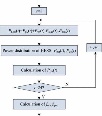
Flow chart of the proposed EMS control and calculation scheme
-
Step 8: Contrast the objective function values of the selected individual with the ones of the crossed candidate individual, and select the stronger individual to enter the next-generation population, which is able to improve the population performance. This selection uses the fitness function in (21) based on the MMDP which is described below.
-
Step 9: Check whether maximum iterations in (11) has been reached. If so, cease iterations; otherwise, go back to Step 5.

3.4 MMDP of fuzzy control
In classical set theory, an element either belongs to a certain set or does not belong to it, and other situations do not exist. The concept of a fuzzy set is different, and the elements on the domain do not absolutely “belong” or “not belong” to a certain set. The degree that elements belong to a certain set is not an absolute 0 or 1, but a real number between 0 and 1 [34].
The concept of a fuzzy set can be described as follows. A mapping \(\mu_{A}\) from the domain U to [0, 1], defines a fuzzy set A of U. If x is an element in A, the membership degree to which x belongs to A is \(\mu_{A} (x)\). If the degree to which x belongs to A is higher, the value of \(\mu_{A} (x)\) is closer to 1; if the degree to which x belongs to A is lower, the value of \(\mu_{A} (x)\) is closer to 0.
Applying this concept to multi-objective optimization, the intersection of the objective functions f i can be expressed as the intersection of fuzzy sets, giving the fuzzy decision set \(D = \mathop \cap \limits_{i = 1}^{m} f_{i}\) where \(i \in (1,2, \ldots ,m)\). Its membership degree function can be expressed as
The definition of the intersection of fuzzy sets is as follows. For three fuzzy sets A, B and C, and x belonging to U, then
and the set C can be regarded as the intersection of A and B, written as \(C = A \cap B\).
According to the MMDP, the following equation can be obtained:
The optimal \(x_{\text{m}}^{ * }\) that has the maximum membership degree of the fuzzy decision set is the optimum solution to the multiple objective functions f i .
In the application of fuzzy set theory, the selection of membership degree functions is very important, and needs to be made according to their characteristics and the optimization model. Common membership degree functions include the normal type and the Γ type. In this paper, the optimization objective of an EMS is to achieve the lower economic costs and higher reliability, that is to say, the objective functions of operating and maintenance cost and LPSP should be kept as low as possible. In this case, the Γ type membership degree function was chosen, and its expression is given here and graphed in Fig. 3:

Curve of Γ type membership degree function
Two objective functions, f 1 for operating and maintenance cost and f 2 for LPSP, are used to construct a fuzzy decision set for optimization by the MMDP. Setting \(\lambda = f_{{\hbox{min}} i} (i = 1,2)\), the membership degree function of \(\mu_{i}\) in the range of (0, 1] is given by
Thus, according to fuzzy control theory, the multi-objective problem of optimal dispatch of a DC microgrid can be converted into the single-objective problem of maximizing the overall membership degree:
where \(\mu (x)\), \(\mu_{1} (x)\) and \(\mu_{2} (x)\) are the overall satisfaction degree, the satisfaction degree of operating and maintenance cost, and the satisfaction degree of LPSP, respectively, when the EMS of a DC microgrid is operated according to solution x.
The solution is to maximize the value of \(\mu (x)\), but the DE algorithm is for minimization. Therefore, maximum membership degree objectives should be converted into minimum value objectives, and consequently the final converted fitness function can be expressed as:
4 Case analysis and simulation results
4.1 Data and parameters of DC microgrid
The following data have been constructed to represent a typical day’s operation of a DC microgrid. The forecast load profile is shown in Fig. 4, and the forecast profiles of solar irradiance, temperature and wind speed are shown in Fig. 5, Fig. 6 and Fig. 7 respectively.

Load profile on typical day

Profile of solar irradiance on typical day

Profile of ambient temperature on typical day

Profile of wind speed on typical day
From these data, using output power modeling for PV and WT generators [32], [33], the power generated by renewable energy in a DC microgrid during a typical day are calculated, as shown in Fig. 8. The output power of PV units varies with solar irradiance, and is zero at night. WT units can generate power both day and night, however, they stop working from 2:00 pm to 4:00 pm because the wind speeds exceed the cut-out wind speed.

Prediction of energy production of PV and WT units in DC microgrid
The type and capacity of DG sources in a microgrid, and the rated power and energy storage capacity of a HESS, can be optimized by using methods such as those described in [35] and [36]. Sizing results for components of an example DC microgrid, their corresponding operating and maintenance costs (O&M C), and SOC limits of a HESS are shown in Table 3. In addition, the value of outage losses (K loss) is estimated as 11 CNY / kWh.
4.2 Pareto fronts of the multi-objective optimization
According to these data and parameters for a DC microgrid, by using the DE algorithm steps presented in Section 3.3, the Pareto front of the multi-objective optimization of an EMS for this DC microgrid can be obtained, and the corresponding objective values are shown in Table 4. They can be chosen as the optimal solution of multi-objective optimization.
As can be seen in Table 4, with lower LPSP, the operating and maintenance cost is higher than for situations with higher LPSP. Therefore, although the results shown in Table 4 are the optimal solutions of multi-objective optimization, it is still necessary to decide where on the Pareto front is the best solution. As described in Section 3, existing methods to select Pareto non-dominated solutions to obtain a final optimization result are significantly influenced by artificial factors.
4.3 Simulation results for EMS based on the MMDP
This paper obtains a unique solution with maximum satisfaction degree according to the proposed approach based on the MMDP. By using the this method and the Pareto front obtained above, the minimum values of operating and maintenance cost and the LPSP can be obtained. The unique solution with the maximum membership degree in this case has operating and maintenance cost f oc = 980.00 CNY and LPSP f lpsp = 1.58%. The corresponding power supply balance for the DC microgrid is shown in Fig. 9, and the power exchanged between the GCC and the main grid is shown in Fig. 10.

Power delivery and demand in DC microgrid by using the proposed MMDP based EMS

Power exchanged through the grid-connected converter
From Fig. 9 and 10, it can be seen that, in the typical day studied, the system has insufficient electricity supply during the hours concluding at 20:00, 21:00 and 23:00. However, the power supply requirements can be satisfied at most of the time. Considering the process of exchanging power between the DC microgrid and the main grid, the influence of the electricity price on operational strategies of the EMS is confirmed. Specifically, at the peak price of the main grid, the DC microgrid is mainly purchasing electricity, and at the valley price it is mainly selling electricity. However, the operational strategies do not strictly synchronize with electricity price fluctuations because the system must primarily meet stability requirements. For example, at the peak price, when the power generated by renewable energy units is not enough to supply the load, purchasing electricity is necessary even though it is relatively expensive at this moment. Similarly, at the valley price, when the power generated by renewable energy units is greater than the load requires, and the system still has available energy after the HESS is charged, even though the price is relatively cheap at this moment, selling electricity selling is the best choice.
The charging and discharging profiles and the normalized SOC of batteries and ultra-capacitors in the HESS are shown in Fig. 11 and Fig. 12. In Fig. 11, positive power means the battery or UC is discharging, and negative power means it is charging.

Charging and discharging power of batteries and ultra-capacitors based on the proposed EMS

SOC of batteries and ultra-capacitors based on the proposed EMS
It can be seen that the output power of the batteries does not have the sudden and large variations because the ultra-capacitors buffer the power fluctuations, and in particular they deliver power to compensate the WT cut-off due to high winds at 14:00. These operating results for the HESS verify the complementary advantages of the batteries and the ultra-capacitors, which help to prolong the life span of the batteries.
5 Conclusion
This paper proposes a multi-objective optimization approach for an EMS in DC microgrids. The DE algorithm is used to obtain the optimal solutions for the EMS according to modeling of a DC microgrid, the power allocation method of a HESS, and constraints of the microgrid components. The operating and maintenance cost and the LPSP are chosen as the EMS optimization objectives. Based on the multi-objective non-dominated sorting method, the Pareto front of the multi-objective optimization can be obtained. Then, by using the MMDP, the best combination of fitness values for operating and maintenance cost and LPSP can be obtained from the Pareto front solutions. Accordingly, the unique solution from the Pareto optimum solution set is achieved, with the maximum overall satisfaction degree for DC microgrid optimized operation.
By considering a typical day of microgrid operation as an example, and according to predictions of load, solar irradiance, wind speed, and temperature, the hourly power output of the renewable energy generation units can be calculated, and the operation of the HESS determined. The power exchanged with the main electricity grid is considered as the optimization variable. The optimum operating solution to optimize the power flows in DC microgrid to achieve economy and reliability is determined using the proposed multi-objective EMS optimisation. The simulation results demonstrate its feasibility and effectiveness.
References
Alegria E, Brown T, Minear E et al (2014) CERTS microgrid demonstration with large-scale energy storage and renewable generation. IEEE Trans Smart Grid 5(2):937–943
Pogaku N, Prodanovic M, Green T (2007) Modeling, analysis and testing of autonomous operation of an inverter-based microgrid. IEEE Trans Power Electron 22(2):613–625
Venkataramanan G, Marnay C (2008) A larger role for microgrids. IEEE Power Energy Mag 6(3):78–82
Li Y, Nejabatkhah F (2014) Overview of control, integration and energy management of microgrids. J Modern Power Syst Clean Energy 2(3):212–222. doi:10.1007/s40565-014-0063-1
Li Q, Xu Z, Yang L (2014) Recent advancements on the development of microgrids. J Modern Power Syst Clean Energy 2(3):206–211. doi:10.1007/s40565-014-0069-8
Koohi-Kamali S, Rahim NA, Mokhlis H (2014) Smart power management algorithm in microgrid consisting of photovoltaic, diesel, and battery storage plants considering variations in sunlight, temperature, and load. Energy Convers Manag 84:562–582
Mehrasa M, Pouresmaeil E, Mehrjerdi H et al (2015) Control technique for enhancing the stable operation of distributed generation units within a microgrid. Energy Convers Manag 97:362–373
Etxeberria A, Vechiu I, Camblong H et al (2014) Operational limits of a three level neutral point clamped converter used for controlling a hybrid energy storage system. Energy Convers Manag 79:97–103
Solanki B, Bhattacharya K, Cañizares C (2017) A sustainable energy management system for isolated microgrids. IEEE Trans Sustain Energy 8(4):507–1517
Pavan Y, Bhimashingu R (2015) Renewable energy based microgrid system sizing and energy management for green buildings. Journal of Modern Power System and Clean Energy 3(1):1–13. doi:10.1007/s40565-015-0101-7
Guerrero J, Loh P, Lee T et al (2017) Advanced control architectures for intelligent microgrids—part II: power quality, energy storage, and AC/DC microgrids. IEEE Trans Ind Electron 60(4):1263–1270
Shi W, Xie W, Chu C et al (2015) Distributed optimal energy management in microgrids. IEEE Trans Smart Grid 6(3):1137–1146
Bracco S, Delfino F, Pampararo F et al (2015) A dynamic optimization-based architecture for polygeneration microgrids with tri-generation, renewables, storage systems and electrical vehicles. Energy Convers Manag 96:511–520
Gupta RA, Gupta NK (2015) A robust optimization based approach for microgrid operation in deregulated environment. Energy Convers Manag 93:121–131
Karavas CS, Kyriakarakos G, Arvanitis KG et al (2015) A multi-agent decentralized energy management system based on distributed intelligence for the design and control of autonomous polygeneration microgrids. Energy Convers Manag 103:166–179
Olivares D, Lara J, Cañizares C et al (2015) Stochastic-predictive energy management system for isolated microgrids. IEEE Trans Smart Grid 6(6):2681–2693
Kakigano H, Miura Y, Ise T (2010) Low-voltage bipolar-type dc microgrid for super high quality distribution. IEEE Trans Power Electron 25(12):3066–3075
Chen YK, Wu YC, Song CC et al (2013) Design and implementation of energy management system with fuzzy control for DC microgrid systems. IEEE Trans Power Electron 28(4):1563–1570
Wang B, Sechilariu M, Locment F (2013) Intelligent DC microgrid with smart grid communications: control strategy consideration and design. IEEE Trans Smart Grid 3(4):2148–2156
Che L, Shahidehpour M (2014) DC microgrids: economic operation and enhancement of resilience by hierarchical control. IEEE Trans Smart Grid 5(5):2517–2526
Sechilariu M, Wang BC, Locment F et al (2014) DC microgrid power flow optimization by multi-layer supervision control: design and experimental validation. Energy Convers Manag 82:1–10
Naresh G, Raju MR, Narasimham SVL et al (2014) Design of clonal selection algorithm based PSS for damping power system oscillations. In: Smart electric grid (ISEG) international conference, Guntur, India, 19-20 September 2014, pp 1–7
Al-Saedi W, Lachowicz SW, Habibi D et al (2013) Power flow control in grid-connected microgrid operation using particle swarm optimization under variable load conditions. Int J Electr Power Energy Syst 49(1):76–85
Hejazi HA, Mohabati HR, Hosseinian SH et al (2011) Differential evolution algorithm for security-constrained energy and reserve optimization considering credible contingencies. IEEE Trans Power Syst 26(3):1145–1155
Baatar N, Minh-Trien P, Chang-Seop K (2013) Multiguiders and nondominate ranking differential evolution algorithm for multiobjective global optimization of electromagnetic problems. IEEE Trans Magn 49(5):2105–2108
Chakraborty S, Ito T, Senjyu T et al (2013) Intelligent economic operation of smart-grid facilitating fuzzy advanced quantum evolutionary method. IEEE Trans Sustain Energy 4(4):905–916
Yan C, Hui Y, Ning L (2010) Weight coefficient cluster covering genetic algorithm for multi-objective optimization based on accurate and fuzzy decoding. In: Second Pacific-Asia conference on circuits,communications and system, Beijing, China, 1-2 August 2010: 269-272
Hui W, Feng Q (2008) Improved PSO-based multi-objective optimization using inertia weight and acceleration coefficients dynamic changing, crowding and mutation. In: 7th world congress on intelligent control and automation, Chongqing, China, 25–27 June 2008, pp 4479–4484
Das S, Abraham A, Konar A (2008) Automatic clustering using an improved differential evolution algorithm. IEEE Trans Syst Hum 38(1):218–237
Guo G, Li W, Yang B et al (2012) Predicting pareto dominance in multi-objective optimization using pattern recognition. In: Proceedings of 2012 international conference on intelligent system design and engineering applications, Sanya, Hainan, China, 6-7 January 2012, pp 456–459
Man-Im A, Ongsakul W, Singh JG et al (2014) Multi-objective economic dispatch considering wind generation uncertainty using non-dominated sorting particle swarm optimization. In: International conference and utility exhibition on green energy for sustainable development, Pattaya, Tailand, 19–21 March 2014, pp 1–6
Fossati JP, Galarza A, Martín-Villate A et al (2015) A method for optimal sizing energy storage systems for microgrids. Renew Energy 77:539–549
Meiqin M, Peng J, Liuchen C et al (2014) Economic analysis and optimal design on microgrids with SS-PVs for industries. IEEE Trans Sustain Energy 5(4):1328–1336
Han-Xiong L, Gatland HB (1996) Conventional fuzzy control and its enhancement. IEEE Trans Cybern 26(5):791–797
Yang H, Zhou W, Lu L et al (2008) Optimal sizing method for stand-alone hybrid solar-wind system with LPSP technology by using genetic algorithm. Sol Energy 82(4):354–367
Moradi MH, Eskandari M, Hosseinian SM (2015) Operational strategy optimization in an optimal sized smart microgrid. IEEE Trans Smart Grid 6(3):1087–1095
Acknowledgements
This work was supported by National Natural Science Foundation of China (No. 51707045).
Author information
Authors and Affiliations
Corresponding author
Additional information
CrossCheck date:11 July 2017
Rights and permissions
Open Access This article is distributed under the terms of the Creative Commons Attribution 4.0 International License (http://creativecommons.org/licenses/by/4.0/), which permits unrestricted use, distribution, and reproduction in any medium, provided you give appropriate credit to the original author(s) and the source, provide a link to the Creative Commons license, and indicate if changes were made.
About this article

Cite this article
WANG, P., WANG, W., MENG, N. et al. Multi-objective energy management system for DC microgrids based on the maximum membership degree principle. J. Mod. Power Syst. Clean Energy 6, 668–678 (2018). https://doi.org/10.1007/s40565-017-0331-y
Received:
Accepted:
Published:
Issue Date:
DOI: https://doi.org/10.1007/s40565-017-0331-y