
Abstract
Active distribution network (ADN) is a solution for power system with interconnection of distributed energy resources (DER), which may change the network operation and power flow of traditional power distribution network. However, in some circumstances the malfunction of protection and feeder automation in distribution network occurs due to the uncertain bidirectional power flow. Therefore, a novel method of fault location, isolation, and service restoration (FLISR) for ADN based on distributed processing is proposed in this paper. The differential-activated algorithm based on synchronous sampling for feeder fault location and isolation is studied, and a framework of fault restoration is established for ADN. Finally, the effectiveness of the proposed algorithm is verified via computer simulation of a case study for active distributed power system.
1 Introduction
With the development of technology in power system, the use of cleaner energy for power generation and closer generation point to the user side has become a new trend in solving the environment problem [1]. Renewable energy generations, especially wind power and solar photovoltaic (PV) generations are among the most effective technologies in generating electricity from distributed energy resources (DER) [2–4]. Therefore, with the mass of DER connected to distribution network in the future, how to use these clean energy sources more effectively and to ensure safe operation of power system will become new research directions. A micro-grid is a cluster of distributed generators and loads operating under different conditions [5]. The distribution networks, which are connected with embedded generators and active controls, are termed as an active distribution network (ADN) [6]. ADN is a new applicable way to change the traditional grid operation of radial distribution mode. It allows bidirectional power flow of grid operation even with the appearance of “Intended Island” [7]. Therefore, it will recover more load loss after system fault, and enhance the reliability of the entire power system.
As an important part of the distribution network, the construction of the distribution automation brings new challenges and also chances to the development of the traditional ADN [8–10]. The technology of FLISR provides directive and efficient solution to improve the reliability of the power system, and gives great significance to the enhancement of supply capacity, as well as efficient and economical operation of the grid [11–13].
The requirement of continuous improvement of power supply reliability and the demand of users increase with the development of the ADN. As one of the approaches of FLISR, distributed processing method is a way to isolate fault points and to restore regional power relying on mutual cooperation between devices, and lack complete solution in ADN [14–16].
ADN is a distribution network system with the inclusion of capability of intended island operation and higher self-healing, which not only takes full advantage of continuous power supply of DER, but also improves power system reliability even when fault occurs. A new FLISR for ADN based on distributed processing method is presented in this paper, which meets the need of ADN.
2 Differential-activated protection algorithm in active distribution network protection
2.1 Fault current analysis of active distribution network
With the interconnection of DER in distribution network, short-circuit current will be added to the fault point when it occurs, which leads to changes of both the operation of traditional radial distribution grid and the distribution of fault current. As for the protection, the fault current provided by the DER is only taken into consideration during the occurrence of the fault, so that the distributed power resource can be presented as a model of power supply with series reactance. There are three circumstances for DER interconnected with ADN during fault happens listed as follows.
-
1)
Situation 1: If the current protection is located at the upstream of DER, and the short-circuit fault occurs at the upstream of DER. The equivalent circuit diagram is shown in Fig. 1.
Fig. 1 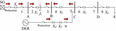
Equivalent circuit diagram of distribution network with DER in situation 1
If fault occurs at f 1, the short-circuit current of protection 2 and 4 are as follows:
$$I_{k1} = \frac{{E_{s} }}{{X_{s} + \alpha X_{1} }}$$(1)$$I_{4} = \frac{{E_{d} }}{{X_{d} + X_{T} + X_{2} + (1 - \alpha )X_{1} }}$$(2)where \(E_{s}\) is equivalent point voltage of power supply in distribution network; \(E_{d}\) the equivalent point voltage of DER; \(\alpha\) the percentage of the fault location between line AB; \(X_{s}\) the equivalent impedance of power supply in distribution network; \(X_{d}\) the equivalent impedance of DER; \(X_{T}\) the equivalent impedance from the DER location to point C; \(X_{1}\) the equivalent impedance of line AB; and \(X_{2}\) the equivalent impedance of line BC.
It can be seen from (1), (2), and Fig. 1 that the fault current of protection 2 is the same no matter whether the DER is considered in the distribution network. However, the DER will provide fault current from the reverse direction of protection 4, due to the non-consideration of phase angle in over-current protection, which may cause malfunction in distribution network.
-
2)
Situation 2: If the current protection is located at the upstream of DER, and the short-circuit fault occurs at the downstream of DER. The equivalent circuit diagram is shown in Fig. 2.
$$I_{2} = I_{4} = \frac{{E_{s} - \frac{{\frac{{E_{s} \left( {X_{d} + X_{T} } \right) + E_{d} \left( {X_{s} + X_{1} + X_{2} } \right)}}{{X_{s} + X_{1} + X_{2} + X_{d} + X_{T} }}}}{{\frac{{\left( {X_{d} + X_{T} } \right)\left( {X_{s} + X_{1} + X_{2} } \right)}}{{X_{s} + X_{1} + X_{2} + X_{d} + X_{T} }} + \gamma X_{3} }}\gamma X_{3} }}{{X_{1} + X_{2} }}$$(3)where \(\gamma\) is percentage of the fault location between line CD; and \(X_{3}\) the equivalent impedance of line CD.
Fig. 2 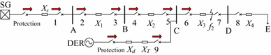
Equivalent circuit diagram of distribution network with DG in situation 2
It can be seen from (3) and Fig. 2 that the fault current of both protection 2 and 4 will decline due to the access of DER, which may reduce the protection sensitivity and lead to fault in protection activation, thanks to the decrease of the protection area.
-
3)
Situation 3: If the current protection is located at the downstream of DER, and the short-circuit fault occurs at the downstream of DER. The equivalent circuit diagram is shown in Fig. 3.
$$I_{6} = \frac{{\frac{{E_{s} \left( {X_{d} + X_{T} } \right) + E_{d} \left( {X_{s} + X_{1} + X_{2} } \right)}}{{X_{s} + X_{1} + X_{2} + X_{d} + X_{T} }}}}{{\frac{{\left( {X_{d} + X_{T} } \right)\left( {X_{s} + X_{1} + X_{2} } \right)}}{{X_{s} + X_{1} + X_{2} + X_{d} + X_{T} }} + \gamma X_{3} }}$$(4)Fig. 3 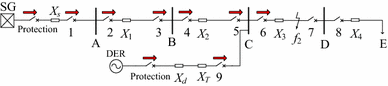
Equivalent circuit diagram of distribution network with DG in situation 3
It can be seen from (4) and Fig. 3 that the fault current of Protection 6 is increased due to the access of DER, which may lead to fault in protection activation, due to the increase of the protection area.


2.2 Differential-activated algorithm based on synchronous sampling
As traditional over-current protection cannot meet the demand of ADN. New method of protection is in need to be introduced. However, with the consideration of the high implementation difficulty of extensive installation of voltage transformer (VT) to collect the voltage signal, the differential-activated algorithm based on synchronous sampling is of significance to meet the demand of protection technology in ADN.
As for current signal at base frequency \(x(t) = \sqrt 2 X\;\sin \left( {\omega t + \varphi } \right)\), it takes two sample sets in real-time measurement:
where N is window length of the sampling data; and r is any random time during the measurement.
Transform the equation above as:
then (12) is the recursive algorithm iterative formula of DFT
that is:
where \(N\theta = 2\pi\)
Note that, as for sinusoidal variable at base frequency, the phase calculated through (14) is a fixed vector in the complex plane. Therefore, the phase difference of two or even more ends of the feeder section can be delivered accurately at any given moment. The phase difference will be calculated through complex operation. The real and imaginary parts of the current signal at base frequency can be described as:
According to the analysis in section 2.1, the current of switch 1 and that of the outlet switch in non-fault area in situation 1 is exactly the same with the current of adjacent switch 2 in fault area.
Since \(I_{\text{protection}} = I_{1} = I_{2} = \frac{{E_{s} }}{{X_{s} + \alpha X_{1} }}\), the phase angle difference of each current is 0°. Likewise, the current of switch 4, switch 5 and switch 9, as well as that of the interconnecting switch in the non-fault area, which is supplied by the DER on the backside, is the same as the current of adjacent switch 3 in fault area.
\(I_{\text{protection}} = I_{3} = I_{4} = I_{5} = I_{9} = \frac{{E_{d} }}{{X_{d} + X_{T} + X_{2} + (1 - \alpha )X_{1} }}\), thus the angle difference of adjacent current is 0°. However, as the result of the synchronization of DER before the occurrence of fault, the voltage amplitude and phase angle of switch 2 and switch 3 in the fault area should remain the same. In this case, we assume \(E_{s} = E_{d}\) . In the same time, the equivalent impedance of external distribution network \(X_{s}\) can also be negligible compared to the line impedance of distribution network. In the distribution network, the resistance/inductance of overhead line is approximately equal to 1, and the resistance/inductance of the cable is slightly less than 1, so that the impedance angle of \(X_{s} + X_{1}\) and \(X_{d} + X_{T} + X_{2} + (1 - \alpha )X_{1}\) should be around 45°, that is: the current direction of \(I_{2} = \frac{{E_{s} }}{{X_{s} + \alpha X_{1} }}\) and \(I_{3} = \frac{{E_{d} }}{{X_{d} + X_{T} + X_{2} + (1 - \alpha )X_{1} }}\) is opposite, and the phase angle difference should be within the error range of 180°.
Since large capacitance to ground occurs in actual distribution operated lines and cables, during the occurrence of fault, capacitive current appears at both ends in fault point, which leads to significant fluctuations of fault current phases both ends. The fault identification algorithm below will take its impact in the error fluctuation into consideration.
In the fault identification algorithm, the waveform of fault current before and after is mutually transferred by way of peer-to-peer communication. Through calculation and comparison, within the actual devices, set 64 points in 1 cycle, and the sampling frequency of 3200 Hz, thus reducing the wave curve by first-order low-pass filter. Considering the application of 0 s instant current protection, the current phase angle after the occurrence of the fault can be calculated through 0.5 s current waveform before the moment of switch trips. The both ends of the fault current phase angle are calculated as:
Thus the location of the fault can be deduced from the current amplitude \(I_{1}\), \(I_{2}\), and the phase angle \(\theta_{1}\), \(\theta_{2}\) of different ends of the power line as follows. The schematic diagram of differential-activated algorithm is shown in Fig. 4.

Schematic diagram of differential-activated algorithm
-
1)
Identify the occurrence of overcurrent fault signal at the outlet switch. If so, the protection trips, and start the algorithm to determine the fault area. Meanwhile, the outlet switches communicate with the adjacent switch, and pass the current waveform as well as over-current signal.
-
2)
Determine whether the two adjacent switches are undertaking overflow. If positive, then move to the next step. If the switch on one side of the feeder section is bearing over-current and the other is not, then the fault is located between the two ends of this feeder section, and these switches must be disconnected. If none of the switches is undertaking over-current, then the fault is not located within this line, and it will be another adjacent switch to be explored.
-
3)
Through the current waveform of the adjacent switches before and after the fault, \(I_{1R}\), \(I_{1I}\), \(I_{2R}\) and \(I_{2I}\) are calculated as \(\theta_{1} = tg^{ - 1} (I_{1R} /I_{1I} )\), \(\theta_{2} = tg^{ - 1} (I_{2R} /I_{2I} )\), and the phase angle is calculated through the fault current waveform sampled from the two ends of the line. If \(|\theta_{1} - \theta_{2} | \in (180^{ \circ } - \delta ,\;180^{ \circ } + \delta )\), and \(\delta\) refers to the actual error coefficient, taking consideration of the current phase fluctuations caused by line-to-ground capacitance. Then the fault is located within this feeder section. Otherwise, it is other adjacent switches to seek.
-
4)
Continue to search for the downstream adjacent switch and repeat the process 2) and 3), until the fault area is found. Open all the switches in this area, end the algorithm, and the fault is isolated.
3 Framework of distributed processing FLISR in active distribution network
The most difference between ADN and traditional distribution network is the interconnection of DER. When there is a fault occuring in ADN, DER will provide short-circuit current to the short point. That is the reason traditional feeder automation cannot work due to DER provides short-circuit current.
A schematic diagram of ADN is used in Fig. 5. First, a fault is happened between load switch 4 and 5. There are two DER interconnect with ADN through switch 3 and 6. Breaker 1 is a feeder outlet switch. Switch 7 is a tie switch. If there is no DER interconnected, and the fault is still happened between switch 4 and switch 5, then breaker 1 and switch 2 and switch 4 is over-current, switch 5 and 7 is non over-current. The traditional feeder automation can find the last over-current switch from outlet switch because distribution network is a radial structure. Then the fault is located between switch 4 and 5. Since there are two DERs interconnected with ADN, it will change the short circuit current. Also, faults happened in ADN due to DER may have an isolate landing protection that can protect DER from fault happened. All of three situations are presented due to isolate landing protection from DER in ADN.

Schematic diagram of ADN
-
1)
Situation 1: none of isolate landing protection is activated.
-
2)
Situation 2: one of isolate landing protection is activated.
-
3)
Situation 3: all of isolate landing protection is activated.
In the above situations, whether the DER provides short-circuit current is judged by the activation of the isolation protection during the fault. In the meantime, some DER cannot provide large amount of energy because of self-capacity, thus the over-current signal may not be detected because short-circuit current may be too small. As for such situation, especially where the short-circuit current cannot be detected, take the reason of non-supply of short-circuit current by DER as the activation of the isolation protection like that in situation 2 and 3. If all the DER in the distribution coincide with the situation mentioned above, then the distribution is regarded as situation 3; if part of the DER comply with the situation mentioned above, then the distribution network is regarded as situation 2; if there is no DER match the situation above, the distribution network is regarded as situation 1.
Although the DG capacity in the access of ADN may be too small, and the outlet current during the fault may be too small to catch the over-current signal at the switch at the DG side, the protection can be activated simply by the over-current signal at the outlet switch, but not in need of loss-of-voltage signal at every switch, for that distributed FA process is applied in this paper, and the launch condition is operated after the activation of outlet protection of the fault. Therefore, the differential-activated protection algorithm proposed previously should be applicable to the three situations mentioned above, specifically as follows.
-
1)
Situation 1: DERs provide short circuit current to short point, so switch 3, 5 and 6 are over-current. The traditional feeder automation is disutility. A differential-activated protection algorithm is presented in section 3 to solve fault location problem. It can solve the situation like this since the short-circuit fault occurs at the upstream of one DER, and the short-circuit fault occurs at the downstream of another DER. Assume the protection in feeder outlet breaker is a 0 s current fast-tripping protection, then the distributed processing FLISR for ADN is shown in Table 1.
Table 1 Schematic diagram of ADN in situation 1 -
2)
Situation 2: While one DER provides short circuit current through switch 3 to short point and another DER cannot provide short circuit current, so switch 3 is over-current. Switch 5 and 6 is non over-current. In another situation, while one DER provides short circuit current through switch 6 to short point and another DER cannot provide short circuit current, then switch 5 and 6 is over-current. Switch 3 is non over-current. Both situations can be solved by the algorithm presents in chapter 3. So it is the same as situation 1 and the feeder automation for ADN is just the same as shown in Table 1. So we choose one DER provides short circuit current through switch 3 to short point and another DER can’t provide short circuit current, the distributed processing FLISR for ADN is shown in Table 2.
Table 2 Schematic diagram of ADN in situation 2 -
3)
Situation 3: None of DERs provides short circuit current to short point, so switch 3, 5 and 6 is non over-current. It is just like the traditional distribution network. Therefore, the traditional feeder automation is utility. The algorithm presented in Section 3 is also effective. T he distributed processing FLISR for ADN in situation 3 is shown in Table 3.
Table 3 Schematic diagram of ADN in situation 3
Through the above-mentioned analysis, the framework of distributed processing FLISR presented in paper for ADN is effective in all three situations.
4 Fault recovery method of active distribution network
Principles of smart fault restoration in ADN are established in this paper. Different types of fault will give rise to disparity in the range of power outage and load loss requiring to be transferred. Therefore, the approach to solve such problems is to take the worst situation into account, where the fault is located at the outlet side of the transformer substation and full load of this feeder is powered off.
In multi-connected and multi-branch distribution network, IEEE 1547-2003 provides that DER cannot supply power as an isolated island after its access to the distribution network. In such case, the breaker-connecting DER to distribution power system can only be considered as a load switch rather than outlet circuit breaker. In consequence, the DER cannot be regarded as a new power source point in the network during the process of fault recovery, but a negative power load as in the traditional multi-connected and multi-branch distribution network.
After the switch tripping of the feeder outlet due to the fault, the smart distributed feeder automation mentioned in this paper will send fault alert signal from downstream feeder switch, and seek tie-switches through peer-to-peer communication with adjacent switches. In this way, the fault restoration process is activated by the fault location signal received by possibly connected switches. Every switch in the breakdown area will obtain the complete information of its connected switches during the fault. Fault restoration in multi-power-supply distribution network is accomplished through such algorithm in which one and only switch set is judged to be enclosed.
Assume the entire loss load in the fault area is transferred to one of the candidate feeders sought from the tie-switches mentioned before. If the remaining power supply capacity of this feeder cannot meet the need of that of loss load in the fault area minus the DER capacity, then assume the DER as a negative load. Under such assumption, whether the capacity of that load loss minus DER meets the need of the remaining loss capacity is to be calculated. If the capacity is met, then move on to the downstream switch to operate recursive calculation until the remaining capacity is not met anymore. Set the switch that cannot meet the need as a new tie-switch, and put its downstream powered-off area back into the recovery section of the proposed algorithm above to operate calculation, in order to reach a new fault restoration scheme.
Fault identification and immediate isolation is implemented by the differential-activated algorithm based on synchronous sampling proposed in section 2.2. Afterwards whether the recovery scheme can meet the loss capacity is calculated by the fault recovery method presented in this section, judged by the algorithm of tie-switch set. Fault restoration for ADN is achieved through the process mentioned above, as shown in Fig. 6.

Schematic diagram of fault restoration for ADN
5 Case study
The whole process is simulated via DIgSILENT within the sample application installed in the National Demonstration Zone in Guizhou, as shown in Fig. 7. The fault point is located between breaker 3 and load switch 8, and types of DER include power storage, PV, wind power, charging pile, hydropower, and cogeneration of cool, heat, and power. The result can be shown in the simulation of three-phase short circuit fault by the criteria mentioned in section 2.2 as in Table 4.

Schematic diagram of the National Demonstration Zone in Guizhou
First, judge from Table 4 whether the current of adjacent switches is overflowing. If over-current is confirmed, then judge the phase angle. Set \(\delta\) as 25° in consideration of the error from actual device acquisition and synchronous sampling. Identification can be made that the fault is located at breaker 3 and load switch 8, which should be switched off and isolated.
In the process of fault recovery, load switch 5 and 7 are searched out first and the remaining capacity is to be examined of these feeders.
With the usage of the fault recovery method proposed in section 5, whether the remaining load capacity is able to meet loss load, which is the power outage load minus load capacity of DER, is recursively calculated from interconnecting switch 5 and 7 to adjacent switches. Take switch 7 as an example, assume its contralateral feeder is able to transfer 2 load capability, and each DER load capacity is 0.15. The peer to peer communication with adjacent switch 10 shows that the load to be recovered is (4 − 0.15 × 6) = 3.1 load capacity. In this case, switch 7 cannot meet the load demand of its contralateral feeder, and recursive calculation is to be applied on switch 10 to get the load capacity. Switch on switch 7, and switch off switch 10 as interconnecting switch, and the capacity of its contralateral feeder minus the load capacity as new capacity to be recovered, and the results are shown in Table 5.
The algorithm cannot continue depth recursive search, therefore, the fault recovery plan drawn by contralateral feeders connected with tie switch 7 is achieved. Finally the new tie switch is load switch 17 that is the last time parent node when the depth of the search is successful. Since contralateral feeder connect with the tie switch 7 cannot recover the entire area lost power supply, tie switch 5 will continue to start power restoration algorithm when the load switch 17 become the new tie switch, empathy recursive results can be obtained in Table 6.
Finally, the result is that the tie switch 5 is closed when depth recursive search algorithm is completed, and the lost power of the whole area will all be restored. Based on the result, the solution of smart distributed power restoration of distribution network interconnected with DER is presented.
Final fault restoration scheme is reached from the recursive calculations of remaining load capacity to undertake from the tie-switch to its adjacent switches, in order to meet the load loss to be transferred, which is the capacity of the loss load in the blackout area minus that of the DER, where load switch 5 and 7 are switched on, in the replacement of the cut-off of breaker 3 and load switch 8 because of fault isolation. Load switch 17 is switched off to separate the powered-off feeders into two parts, and the loss load is re-supplied by two peer feeders.
The distribution network has experienced a great change due to DER contributed short circuit after they interconnected with distribution network. It is need to put forward the corresponding protection measures and distribution automation. This paper proposed a distributed processing FLISR scheme on the basis of current, which is made up of differential-activated protection algorithm. The proposed protection methods are consistent with the development of future distribution network.
6 Conclusion
With the interconnection of DER and change of operation and control modes in the ADN, the traditional feeder automation method encounters the difficulty. This paper proposed a new distributed processing FLISR method for ADN on the basis of current angle, which is made up of differential-activated algorithm based on synchronous sampling. The proposed FLISR algorithm can solve the bidirectional power flow problem brought by DER output. Moreover, the distributed processing mode makes better adaptability to deal with the uncertainty of DER output than the centralized mode.
References
Ustun TS, Ozansoy C, Ustun A (2013) Fault current coefficient and time delay assignment for microgrid protection system with central protection unit. IEEE Trans Power Syst 28(2):598–606
Dong ZY (2013) Guest editorial: special issue on generation and integration technologies for renewable energy. J Mod Power Syst Clean Energy 1(3):203. doi:10.1007/s40565-013-0038-7
Yu WP, Liu D, Weng JM (2013) A power restoring model for distribution network containing distributed generators and improved greedy algorithm. Automat Electr Power Syst 37(24):23–30. doi:10.7500/AEPS201210172 (in Chinese)
Yu WP, Liu D, Huang YH (2015) Load transfer and islanding analysis of active distribution network. Int Trans Electr Energy Syst 25(8):1420–1435
Li YW, Nejabatkhah F (2014) Overview of control, integration and energy management of microgrids. J Mod Power Syst Clean Energy 2(3):212–222. doi:10.1007/s40565-014-0063-1
Esau Z, Jayaweera D (2014) Reliability assessment in active distribution networks with detailed effects of PV systems. J Mod Power Syst Clean Energy 2(1):59–68
Borghetti A, Nucci CA, Paolone M et al (2011) Synchronized phasors monitoring during the islanding maneuver of an active distribution network. IEEE Trans Smart Grid 2(1):82–91
Jouybari-Moghaddam H, Hosseinian SH, Vahidi B (2012) An introduction to active distribution networks islanding issues. In: Proceedings of the 17th conference on electrical power distribution networks (EPDC’12), Tehran, Iran, 2–3 May 2012, 6 pp
Belloni F, Chiumeo R, Gandolfi C et al (2012) A protection coordination scheme for active distribution networks. In: Proceedings of the 47th international universities power engineering conference (UPEC’12), London, UK, 4–7 Sept 2012, 6 pp
Zayandehroodi H, Mohamed A, Shareef H et al (2012) A novel protection coordination strategy using back tracking algorithm for distribution systems with high penetration of DG. In: Proceedings of the 2012 IEEE international power engineering and optimization conference (PEDCO’12), Melaka, Malaysia, 6–7 Jun 2012, pp 187–192
Zeineldin HH, Mohamed YR, Khadkikar V et al (2013) A protection coordination index for evaluating distributed generation impacts on protection for meshed distribution systems. IEEE Trans Smart Grid 4(3):1523–1532
Hussain B, Sharkh SM, Hussain S et al (2013) An adaptive relaying scheme for fuse saving in distribution networks with distributed generation. IEEE Trans Power Deliv 28(2):669–677
Ustun TS, Ozansoy C, Zayegh A (2013) Differential protection of microgrids with central protection unit support. In: Proceedings of the 2013 IEEE TENCON spring conference, Sydney, Australia, 17–19 Apr 2013, pp 15–19
Moreno JG, Perez FE, Orduna EA (2012) Protection functions for distribution networks with distributed generation applying wavelet transform. In: Proceedings of the 6th IEEE PES Latin America transmission and distribution conference and exposition (T&D-LA’12), Montevideo, Uruguay, 3–5 Sept 2012, 5 pp
Batista OE, Flauzino RA, de Moraes LA et al (2013) The faults variability in distribution systems with distributed generation and robustness of smart grids. In: Proceedings of the 2013 IEEE PES conference on innovative smart grid technologies Latin America (ISGT LA’13), Sao Paulo, Brazil, 15–17 Apr 2013, 6 pp
Ling WS, Liu D, Yang DX et al (2015) The situation and trends of feeder automation in China. Renew Sustain Energy Rev 50:1138–1147
Acknowledgment
This paper was supported by the National High Technology Research and Development Program of China (863 Program) (No. 2014AA051902).
Author information
Authors and Affiliations
Corresponding author
Additional information
CrossCheck date: 26 August 2015
Rights and permissions
Open Access This article is distributed under the terms of the Creative Commons Attribution 4.0 International License (http://creativecommons.org/licenses/by/4.0/), which permits unrestricted use, distribution, and reproduction in any medium, provided you give appropriate credit to the original author(s) and the source, provide a link to the Creative Commons license, and indicate if changes were made.
About this article

Cite this article
WENG, J., LIU, D., LUO, N. et al. Distributed processing based fault location, isolation, and service restoration method for active distribution network. J. Mod. Power Syst. Clean Energy 3, 494–503 (2015). https://doi.org/10.1007/s40565-015-0166-3
Received:
Accepted:
Published:
Issue Date:
DOI: https://doi.org/10.1007/s40565-015-0166-3