Correlation coefficient measures and aggregation operators on interval-valued linear Diophantine fuzzy sets and their applications

Abstract

Intuitionistic fuzzy sets, Pythagorean fuzzy sets, and q-rung orthopair fuzzy sets are rudimentary concepts in computational intelligence, which have a myriad of applications in fuzzy system modeling and decision-making under uncertainty. Nevertheless, all these notions have some strict restrictions imposed on the membership and non-membership grades (e.g., the sum of the grades or the sum of the squares of the grades or the sum of the qth power of the grades is less than or equal to 1). To relax these restrictions, linear Diophantine fuzzy set is a new extension of fuzzy sets, by additionally considering reference/control parameters. Thereby, the sum of membership grade and non-membership grade can be greater than 1, and even both of these grades can be 1. By selecting different pairs of reference parameters, linear Diophantine fuzzy sets can naturally categorize concerned problems and produce appropriate solutions accordingly. In this paper, the interval-valued linear Diophantine fuzzy set, which is a generalization of linear Diophantine fuzzy set, is studied. The interval-valued linear Diophantine fuzzy set is more efficient to deal with uncertain and vague information due to its flexible intervals of membership grades, non-membership grades, and reference parameters. Some basic operations on interval-valued linear Diophantine fuzzy sets are presented. We define interval-valued linear Diophantine fuzzy weighted average and interval-valued linear Diophantine fuzzy weighted geometric aggregation operators. Based on these new aggregation operators, we propose a method for multi-criteria decision-making based on supplier selection under the interval-valued linear Diophantine fuzzy environment. Besides, a real-life example, comparison study, and advantages of proposed aggregation operators are presented. We describe some correlation coefficient measures (type-1 and type-2) for the interval-valued linear Diophantine fuzzy sets and they are applied in medical diagnosis for Coronavirus Disease 2019 (COVID-19). Lastly, a comparative examination and the benefits of proposed correlation coefficient measures are also discussed.

1 Introduction

As a generalization of a classical set, Zadeh (1965) brought the perception of a fuzzy set (FS). The membership degrees of elements into a fuzzy set are measured using the membership function. In the literature, Zadeh’s fuzzy set is tackled from different aspects in the multi-criteria decision making (MCDM) issues (Petchimuthu et al. 2020; Petchimuthu and Kamacı 2020, 2019; Ye 2011; Song et al. 2014). The interval-valued fuzzy set (IVFS) is proposed as an interval spanned extension of a fuzzy set (Gehrke et al. 1996; Sambuc 1975). These sets treat the membership degree of a fuzzy set as interval values in place of an exact value. Atanassov (1986) generalized the fuzzy set into the intuitionistic fuzzy set (IFS), which possesses a non-membership grade in addition to membership grade. The perception of IFS is stepped forward to address the real-life MCDM issues (Aydın and Enginog̃lu 2021; Hayat et al. 2018; Kamacı 2019; Karaaslan 2016). The average and geometric aggregation operators are evolved to aggregate the information in the surrounding of IFS [see Xu (2007), Zhao et al. (2010), Xu and Yager (2006)]. To cope with the MCDM issues based on IFS information measures, similarity measures (Song et al. 2014) and cosine similarity measures (Ye 2011) were developed. To expand both the membership and non-membership degrees of the IFS from exact values to interval values, Atanassov and Gargov (1989) brought the interval-valued intuitionistic fuzzy set (IVIFS). Many researchers contributed to the development of IVIFS by proposing aggregation operators (Wang et al. 2012; Garg 2016a) and distance measures (Ye 2013; Baccour and Alimi 2019). Yager (2014) adopted the idea of Pythagorean fuzzy set (PyFS) (is also referred to as IFS of type 2) through relaxing some conditions of IFS and advanced a few outstanding aggregation operators termed O-PFWPA and O-PFWPG. To prioritize the options concerning PyFS, many PyF operations, relations, and aggregation operators were developed (Garg 2017; Hashmi and Riaz 2020). Moreover, the distance measures (Firozja et al. 2020; Nguyen et al. 2019; Zhang et al. 2019), divergence measures (Zeng et al. 2019) and cosine function-based similarity measures (Wei and Wei 2018) were proposed to measure between two PyFNs. In Abdullah and Goh (2019), Akram et al. (2020), Khalid et al. (2019), Riaz and Hashmi (2020), many authors endeavored to deal with the fruitful real-life applications of PyFSs. The PyFS was prolonged into the interval-valued Pythagorean fuzzy set (IVPyFS) (Peng 2019; Zhang 2016) and studied in some aspects (Garg 2016b; Li et al. 2018). In 2017, Yager (2017) introduced the q-rung orthopair fuzzy set (q-ROFS) (is also referred to as IFS of type q (where $q\ge 1$)). Later on, Liu and Wang (2018) and Riaz et al. (2020a) focused on the aggregation operators such as q-ROFHWAGA, q-ROFWA, q-ROFWG, and Wang et al. (2019) aimed to measure the similarity between two q-ROFSs. The different perspectives on q-ROFS, which are closer to real-life applications, were presented (Ali 2018; Ali and Mahmood 2022; Mahmood and Ali 2021). Joshi et al. (2018) extended the q-ROFS into an interval-valued q-rung orthopair fuzzy set (IVq-ROFS), and immediately afterward, they were advanced in different directions (Gao et al. 2019). In 2019, Riaz and Hashmi (2019) significantly tested the regulations associated with the membership and non-membership degrees in the structures of FS, IFS, PyFS, and q-ROFS and those obstacles were offered numerically. They introduced the linear Diophantine fuzzy set (LDFS) by including reference parameters to the nature of IFS to take away those obstacles. They put forward that the idea of LDFS will eradicate the constraints in the existing methodologies of other sets and enable the free selection of data in practice. Also, they proved that the space of this set is larger than those of FS, IFS, PyFS, and q-ROFS using the arbitrary property of the reference parameters [see: Theorem 3.3 and Table 18 in Riaz and Hashmi (2019)]. For more details on the hybridizations, algebraic and topological structures of LDFS, the concepts in Almagrabi et al. (2021), Kamacı (2021a, 2021b), Riaz et al. (2020b) can also be reviewed. Moreover, the reference parameter approach utilized by Riaz and Hashmi (2019) on LDFS is a rising fashion to assess alternatives thoroughly and accurately. It sparks in our thoughts that a deep and tricky observation needs to be made on LDFS.

Thus, encouraged by Riaz and Hashmi’s studies on LDFS in Riaz and Hashmi (2019), we focused on the theory of interval-valued linear Diophantine fuzzy set (IVLDFS) in which the degrees of membership, non-membership, and reference parameters are intervals. We know from the prevailing research (Beg and Rashid 2015; Chinram et al. 2021; Riaz and Hashmi 2019) that the average and geometric aggregation operators are the simplest and appropriate approaches to fuse information. So, we seek the solutions to the supplier selection based on IVLDF information by introducing the interval-valued linear Diophantine fuzzy weighted average (IVLDFWA) and interval-valued linear Diophantine fuzzy weighted geometric (IVLDFWG) aggregation operators. Recently, Garg and Rani (2019) proved that the correlation coefficient measure is one of the most critical measures to assist not only in evaluating data entity with another but also show the extent of association between them and their direction. It leads us to define type-1 and type-2 correlation coefficient measures between two IVLDFSs.

The motivation of this paper is (1) to extend the range of IVLDFS, (2) to derive new operations on IVLDFSs, (3) to present some aggregation operators to fuse IVLDF information, (4) to formulate correlation coefficients that measure similarity/distance between two IVLDSs, and (5) to show that the proposed operations, operators, and correlation coefficients can be used to deal with problems such as supplier selection and medical diagnosis. The contributions of this paper are itemized as follows.

• The current concepts such as IFS, PyFS, q-ROFS, LDFS, IVIFS, IVPyFS, and IVq-ROFS have been prosperously applied in different areas, but there are situations in genuine life that cannot be represented by those notions. The LDFS perception of Riaz and Hashmi generalizes the concepts of IFS, PyFS, q-ROFS, LDFS, IVIFS, IVPyFS, and IVq-ROFS with the integration of reference parameters. The reference parameters increase the range of membership and non-membership grades. Further, by changing the physical sense of reference parameters, LDFS can be used effectively in different situations. The perception of IVLDFS that we propose is the more generalized form of the LDFS of Riaz and Hashmi. It has extra functionality in processing the degrees of membership, non-membership, and reference parameters as interval values instead of exact values in evaluation with LDFS.

• The existing arithmetic, geometric, and other aggregation operators created for the subsisting notions IFS, PyFS, q-ROFS, LDFS, IVIFS, IVPyFS, and IVq-ROFS are not relevant to resolve the MCDM quandaries under the IVLDFS environment. Meanwhile, our proposed arithmetic and geometric aggregation operators (IVLDFWA and IVLDFWG) are eligible to resolve the MCDM based on supplier selection under the environment of both the subsisting notions IFS, PyFS, q-ROFS, LDFS, IVIFS, IVPyFS, IVq-ROFS, and the proposed IVLDFS.

• The information measures proposed for the IFS, PyFS, q-ROFS, LDFS, IVIFS, IVPyFS, and IVq-ROFS are special instances of the proposed type-1 and type-2 correlation coefficients of the IVLDFS. Consequently, the type-1 and type-2 correlation coefficients of IVLDFS are felicitous and effective to deal with the authentic-life MCDM issues more accurately than the preexisting ones.

The rest of this study is organized as follows: In Sect. 2, we give the introductory notions and principal properties about the fuzzy set and its prolonged models. In Sect. 3, we present a framework for linear Diophantine fuzzy set theory in which grades of membership, non-membership, and reference parameters are interval values. Also, we discuss relationships between interval-valued linear Diophantine fuzzy sets and the prolonged interval-valued fuzzy sets like IVIFS, IVPyFS, IVq-ROFS. In Sect. 4, we define interval-valued linear Diophantine fuzzy weighted average (IVLDFWA) and interval-valued linear Diophantine fuzzy weighted geometric (IVLDFWG) aggregation operators. Based on these new aggregation operators, we propose a method for the MCDM based on material supplier selection in the interval-valued linear Diophantine fuzzy surrounding. In addition to these, a real-life example, comparison study, and advantages of proposed aggregation operators (IVLDFWA, IVLDFWG) are presented. In Sect. 5, we describe some correlation coefficient measures (type-1 and type-2) for the IVLDFSs and they are applied in medical diagnosis for Coronavirus Disease 2019 (COVID-19). A comparative examination and the benefits of proposed correlation coefficient measures are also discussed. In Sect. 6, the conclusion of this study is summarized.

2 Preliminaries

This section reviews some basic concepts and results related to the fuzzy set and its extended models.

We start this section with Zadeh’s definition of a fuzzy set.

Definition 2.1

(Zadeh 1965) A fuzzy set (FS) ${\mathcal {F}}$ in the universal discourse set ${\mathfrak {X}}$ is defined as follows:

${\mathcal {F}}=\left\{ \left( x_{i}, \left\langle {\mathfrak {M}}_{{\mathcal {F}}}(x_{i})\right\rangle \right) : x_{i}\in {\mathfrak {X}}\right\}$,

where ${\mathfrak {M}}_{{\mathcal {F}}}: {\mathfrak {X}}\rightarrow [0,1]$ represents the membership function of ${\mathcal {F}}$ and the value ${\mathfrak {M}}_{{\mathcal {F}}}(x_{i})$ denotes the degree of membership of $x_{i}\in {\mathfrak {X}}$ into the set ${\mathcal {F}}$. The set of all FSs over the universal discourse set ${\mathfrak {X}}$ is denoted by $FS({\mathfrak {X}})$.

Definition 2.2

(Gehrke et al. 1996; Sambuc 1975) Let ${\mathfrak {I}}^{[0,1]}$ be the set of all closed subintervals of the interval [0, 1]. Then, an interval-valued fuzzy set (IVFS) $\ddot{{\mathcal {F}}}$ in the universal discourse set ${\mathfrak {X}}$ can be described as follows:

$\ddot{{\mathcal {F}}}=\left\{ \left( x_{i}, \left\langle {\mathfrak {M}}_{\ddot{{\mathcal {F}}}}(x_{i})\right\rangle \right) : x_{i}\in {\mathfrak {X}}\right\}$,

where ${\mathfrak {M}}_{\ddot{{\mathcal {F}}}}: {\mathfrak {X}}\rightarrow {\mathfrak {I}}^{[0,1]}$ represents the membership function of $\ddot{{\mathcal {F}}}$ such that ${\mathfrak {M}}_{\ddot{{\mathcal {F}}}}(x_{i})=[{\mathfrak {M}}^{L}_{\ddot{{\mathcal {F}}}}(x_{i}),{\mathfrak {M}}^{U}_{\ddot{{\mathcal {F}}}}(x_{i})]$ and $0\le {\mathfrak {M}}^{L}_{\ddot{{\mathcal {F}}}}(x_{i})\le {\mathfrak {M}}^{U}_{\ddot{{\mathcal {F}}}}(x_{i})\le 1$. The values ${\mathfrak {M}}^{L}_{\ddot{{\mathcal {F}}}}(x_{i})$ and ${\mathfrak {M}}^{U}_{\ddot{{\mathcal {F}}}}(x_{i})$ denote the lower and upper degrees of membership of $x_{i}\in {\mathfrak {X}}$ into the set $\ddot{{\mathcal {F}}}$, respectively. The set of all IVFSs over the universal discourse set ${\mathfrak {X}}$ is denoted by $IVFS({\mathfrak {X}})$.

Definition 2.3

(Atanassov 1986) An intuitionistic fuzzy set (IFS) ${\mathcal {I}}$ in the universal discourse set ${\mathfrak {X}}$ is defined as follows:

${\mathcal {I}}=\left\{ \left( x_{i}, \left\langle {\mathfrak {M}}_{{\mathcal {I}}}(x_{i}),{\mathfrak {N}}_{{\mathcal {I}}}(x_{i}\right) \right\rangle ): x_{i}\in {\mathfrak {X}}\right\}$,

where ${\mathfrak {M}}_{{\mathcal {I}}}: {\mathfrak {X}}\rightarrow [0,1]$ and ${\mathfrak {N}}_{{\mathcal {I}}}: {\mathfrak {X}}\rightarrow [0,1]$ represent the membership function and non-membership function of ${\mathcal {I}}$, respectively. The values ${\mathfrak {M}}_{{\mathcal {I}}}(x_{i})$ and ${\mathfrak {N}}_{{\mathcal {I}}}(x_{i})$ denote the degrees of membership and non-membership of $x_{i}\in {\mathfrak {X}}$ into the set ${\mathcal {I}}$ with the condition $0\le {\mathfrak {M}}_{{\mathcal {I}}}(x_{i})+{\mathfrak {N}}_{{\mathcal {I}}}(x_{i}) \le 1$ for each $x_{i}\in {\mathfrak {X}}$. The hesitation margin, which is the degree of non-determinacy of $x_{i}\in {\mathfrak {X}}$ into the set ${\mathcal {I}}$, is described as ${\mathfrak {H}}_{{\mathcal {I}}}(x_{i})=1-({\mathfrak {M}}_{{\mathcal {I}}}(x_{i})+{\mathfrak {N}}_{{\mathcal {I}}}(x_{i}))$ for each $x_{i}\in {\mathfrak {X}}$. The set of all IFSs over the universal discourse set ${\mathfrak {X}}$ is denoted by $IFS({\mathfrak {X}})$.

Definition 2.4

(Atanassov and Gargov 1989) Let ${\mathfrak {I}}^{[0,1]}$ be the set of all closed subintervals of the interval [0, 1]. Then, an interval-valued intuitionistic fuzzy set (IVIFS) $\ddot{{\mathcal {I}}}$ in the universal discourse set ${\mathfrak {X}}$ is described as follows:

$\ddot{{\mathcal {I}}}=\left\{ \left( x_{i}, \left\langle {\mathfrak {M}}_{\ddot{{\mathcal {I}}}}(x_{i}),{\mathfrak {N}}_{\ddot{{\mathcal {I}}}}(x_{i})\right\rangle \right) : x_{i}\in {\mathfrak {X}}\right\}$,

where ${\mathfrak {M}}_{\ddot{{\mathcal {I}}}}=[{\mathfrak {M}}^{L}_{{\mathcal {I}}}(x_{i}),{\mathfrak {M}}^{U}_{{\mathcal {I}}}(x_{i})]: {\mathfrak {X}}\rightarrow {\mathfrak {I}}^{[0,1]}$ and ${\mathfrak {N}}_{\ddot{{\mathcal {I}}}}=[{\mathfrak {N}}^{L}_{{\mathcal {I}}}(x_{i}),{\mathfrak {N}}^{U}_{{\mathcal {I}}}(x_{i})]: {\mathfrak {X}}\rightarrow {\mathfrak {I}}^{[0,1]}$ represent the membership function and non-membership function of $\ddot{{\mathcal {I}}}$, respectively. The values ${\mathfrak {M}}^{L}_{{\mathcal {I}}}(x_{i})$, ${\mathfrak {M}}^{U}_{{\mathcal {I}}}(x_{i})$ denote the lower and upper degrees of membership of $x_{i}\in {\mathfrak {X}}$ into the set $\ddot{{\mathcal {I}}}$, and the values ${\mathfrak {N}}^{L}_{{\mathcal {I}}}(x_{i})$, ${\mathfrak {N}}^{U}_{{\mathcal {I}}}(x_{i})$ denote the lower and upper degrees of non-membership of $x_{i}\in {\mathfrak {X}}$ into the set $\ddot{{\mathcal {I}}}$. Besides, the following condition is provided: $0\le {\mathfrak {M}}^{U}_{{\mathcal {I}}}(x_{i})+{\mathfrak {N}}^{U}_{{\mathcal {I}}}(x_{i})\le 1$ for each $x_{i}\in {\mathfrak {X}}$. The hesitation margin is evaluated as ${\mathfrak {H}}_{\ddot{{\mathcal {I}}}}(x_{i})=[1-({\mathfrak {M}}^{L}_{\ddot{{\mathcal {I}}}}(x_{i})+{\mathfrak {N}}^{L}_{\ddot{{\mathcal {I}}}}(x_{i})),1-({\mathfrak {M}}^{U}_{\ddot{{\mathcal {I}}}}(x_{i})+{\mathfrak {N}}^{U}_{\ddot{{\mathcal {I}}}}(x_{i}))]$ for each $x_{i}\in {\mathfrak {X}}$. The set of all IVIFSs over the universal discourse set ${\mathfrak {X}}$ is denoted by IVIFS$({\mathfrak {X}})$.

Definition 2.5

(Yager 2014) A Pythagorean fuzzy set (PyFS) ${\mathcal {P}}$ in the universal discourse set ${\mathfrak {X}}$ is defined as follows:

${\mathcal {P}}=\left\{ \left( x_{i}, \left\langle {\mathfrak {M}}_{{\mathcal {P}}}(x_{i}),{\mathfrak {N}}_{{\mathcal {P}}}(x_{i})\right\rangle \right) : x_{i}\in {\mathfrak {X}}\right\}$,

where ${\mathfrak {M}}_{{\mathcal {P}}}, {\mathfrak {N}}_{{\mathcal {P}}}: {\mathfrak {X}}\rightarrow [0,1]$ represent the membership function and non-membership function of ${\mathcal {P}}$, respectively. The values ${\mathfrak {M}}_{{\mathcal {P}}}(x_{i})$ and ${\mathfrak {N}}_{{\mathcal {P}}}(x_{i})$ denote the degrees of membership and non-membership of $x_{i}\in {\mathfrak {X}}$ into the set ${\mathcal {P}}$ with the condition $0\le ({\mathfrak {M}}_{{\mathcal {P}}}(x_{i}))^{2}+({\mathfrak {N}}_{{\mathcal {P}}}(x_{i}))^{2} \le 1$ for each $x_{i}\in {\mathfrak {X}}$. The hesitation margin of $x_{i}\in {\mathfrak {X}}$ is ${\mathfrak {H}}_{{\mathcal {P}}}(x_{i})=\big (1-(({\mathfrak {M}}_{{\mathcal {P}}}(x_{i}))^{2}+({\mathfrak {N}}_{{\mathcal {P}}}(x_{i}))^{2})\big )^{\frac{1}{2}}$. $PyFS({\mathfrak {X}})$ denotes the set of all PyFSs over the universal discourse set ${\mathfrak {X}}$.

Definition 2.6

(Peng 2019; Zhang 2016) Let ${\mathfrak {I}}^{[0,1]}$ be the set of all closed subintervals of the interval [0, 1]. Then, an interval-valued Pythagorean fuzzy set (IVPyFS) $\ddot{{\mathcal {P}}}$ in the universal discourse set ${\mathfrak {X}}$ is presented as follows:

$\ddot{{\mathcal {P}}}=\left\{ \left( x_{i}, \left\langle {\mathfrak {M}}_{\ddot{{\mathcal {P}}}}(x_{i}),{\mathfrak {N}}_{\ddot{{\mathcal {P}}}}(x_{i})\right\rangle \right) : x_{i}\in {\mathfrak {X}}\right\}$,

where ${\mathfrak {M}}_{\ddot{{\mathcal {P}}}}=[{\mathfrak {M}}^{L}_{{\mathcal {P}}}(x_{i}),{\mathfrak {M}}^{U}_{{\mathcal {P}}}(x_{i})]: {\mathfrak {X}}\rightarrow {\mathfrak {I}}^{[0,1]}$ and ${\mathfrak {N}}_{\ddot{{\mathcal {P}}}}=[{\mathfrak {N}}^{L}_{{\mathcal {P}}}(x_{i}),{\mathfrak {N}}^{U}_{{\mathcal {P}}}(x_{i})]: {\mathfrak {X}}\rightarrow {\mathfrak {I}}^{[0,1]}$ represent the membership function and non-membership function of $\ddot{{\mathcal {P}}}$, respectively. The values ${\mathfrak {M}}^{L}_{{\mathcal {P}}}(x_{i})$, ${\mathfrak {M}}^{U}_{{\mathcal {P}}}(x_{i})$ denote the lower and upper degrees of membership of $x_{i}\in {\mathfrak {X}}$ into the set $\ddot{{\mathcal {P}}}$, and the values ${\mathfrak {N}}^{L}_{{\mathcal {P}}}(x_{i})$, ${\mathfrak {N}}^{U}_{{\mathcal {P}}}(x_{i})$ denote the lower and upper degrees of non-membership of $x_{i}\in {\mathfrak {X}}$ into the set $\ddot{{\mathcal {P}}}$. In addition, the following condition is provided: for each $x_{i}\in {\mathfrak {X}}$, $0\le ({\mathfrak {M}}^{U}_{{\mathcal {P}}}(x_{i}))^{2}+({\mathfrak {N}}^{U}_{{\mathcal {P}}}(x_{i}))^{2}\le 1$. For each $x_{i}\in {\mathfrak {X}}$, ${\mathfrak {H}}_{\ddot{{\mathcal {P}}}}(x_{i})=[{\mathfrak {H}}^{L}_{\ddot{{\mathcal {P}}}}(x_{i}),{\mathfrak {H}}^{U}_{\ddot{{\mathcal {P}}}}(x_{i})]=\big [\big (1-(({\mathfrak {M}}^{L}_{\ddot{{\mathcal {P}}}}(x_{i}))^{2}+({\mathfrak {N}}^{L}_{\ddot{{\mathcal {P}}}}(x_{i}))^{2})\big )^{\frac{1}{2}},\big (1-(({\mathfrak {M}}^{U}_{\ddot{{\mathcal {P}}}}(x_{i}))^{2}+({\mathfrak {N}}^{U}_{\ddot{{\mathcal {P}}}}(x_{i}))^{2})\big )^{\frac{1}{2}}\ \big ]$ is termed to be hesitation margin of $x_{i}\in {\mathfrak {X}}$. The set of all IVPyFSs over the universal discourse set ${\mathfrak {X}}$ is denoted by IVPyFS$({\mathfrak {X}})$.

Definition 2.7

(Yager 2017) A q-rung orthopair fuzzy set (q-ROFS) ${\mathcal {Q}}$ in the universal discourse set ${\mathfrak {X}}$ is defined as follows:

${\mathcal {Q}}=\left\{ \left( x_{i},\left\langle {\mathfrak {M}}_{{\mathcal {Q}}}(x_{i}),{\mathfrak {N}}_{{\mathcal {Q}}}(x_{i})\right\rangle \right) : x_{i}\in {\mathfrak {X}}\right\}$,

where ${\mathfrak {M}}_{{\mathcal {Q}}}, {\mathfrak {N}}_{{\mathcal {Q}}}: {\mathfrak {X}}\rightarrow [0,1]$ represent the membership function and non-membership function of ${\mathcal {Q}}$, respectively. The values ${\mathfrak {M}}_{{\mathcal {Q}}}(x_{i})$ and ${\mathfrak {N}}_{{\mathcal {Q}}}(x_{i})$ denote the degrees of membership and non-membership of $x_{i}\in {\mathfrak {X}}$ into the set ${\mathcal {Q}}$ with the condition $0\le ({\mathfrak {M}}_{{\mathcal {Q}}}(x_{i}))^{q}+({\mathfrak {N}}_{{\mathcal {Q}}}(x_{i}))^{q} \le 1$ (where $q\ge 1$) for each $x_{i}\in {\mathfrak {X}}$. The hesitation margin can be evaluated as ${\mathfrak {H}}_{{\mathcal {Q}}}(x_{i})=\big (1-(({\mathfrak {M}}_{{\mathcal {Q}}}(x_{i}))^{q}+({\mathfrak {N}}_{{\mathcal {Q}}}(x_{i}))^{q})\big )^{\frac{1}{q}}$ for each $x_{i}\in {\mathfrak {X}}$. The set of all q-ROFSs over the universal discourse set ${\mathfrak {X}}$ is denoted by q-ROFS$({\mathfrak {X}})$.

Definition 2.8

(Joshi et al. 2018) Let ${\mathfrak {I}}^{[0,1]}$ be the set of all closed subintervals of the interval [0, 1]. Then, an interval-valued q-rung orthopair fuzzy set (IVq-ROFS) $\ddot{{\mathcal {Q}}}$ in the universal discourse set ${\mathfrak {X}}$ is described as follows:

$\ddot{{\mathcal {Q}}}=\left\{ \left( x_{i}, \left\langle {\mathfrak {M}}_{\ddot{{\mathcal {Q}}}}(x_{i}),{\mathfrak {N}}_{\ddot{{\mathcal {Q}}}}(x_{i})\right\rangle \right) : x_{i}\in {\mathfrak {X}}\right\}$,

where ${\mathfrak {M}}_{\ddot{{\mathcal {Q}}}}=[{\mathfrak {M}}^{L}_{{\mathcal {Q}}}(x_{i}),{\mathfrak {M}}^{U}_{{\mathcal {Q}}}(x_{i})]: {\mathfrak {X}}\rightarrow {\mathfrak {I}}^{[0,1]}$ and ${\mathfrak {N}}_{\ddot{{\mathcal {Q}}}}=[{\mathfrak {N}}^{L}_{{\mathcal {Q}}}(x_{i}),{\mathfrak {N}}^{U}_{{\mathcal {Q}}}(x_{i})]: {\mathfrak {X}}\rightarrow {\mathfrak {I}}^{[0,1]}$ represent the membership function and non-membership function of $\ddot{{\mathcal {Q}}}$, respectively. The values ${\mathfrak {M}}^{L}_{{\mathcal {Q}}}(x_{i})$, ${\mathfrak {M}}^{U}_{{\mathcal {Q}}}(x_{i})$ denote the lower and upper degrees of membership of $x_{i}\in {\mathfrak {X}}$ into the set $\ddot{{\mathcal {Q}}}$, and the values ${\mathfrak {N}}^{L}_{{\mathcal {Q}}}(x_{i})$, ${\mathfrak {N}}^{U}_{{\mathcal {Q}}}(x_{i})$ denote the lower and upper degrees of non-membership of $x_{i}\in {\mathfrak {X}}$ into the set $\ddot{{\mathcal {Q}}}$. In addition, the following condition is provided: $0\le ({\mathfrak {M}}^{U}_{{\mathcal {Q}}}(x_{i}))^{q}+({\mathfrak {N}}^{U}_{{\mathcal {Q}}}(x_{i}))^{q}\le 1$ (where $q\ge 1$) for each $x_{i}\in {\mathfrak {X}}$. The hesitation margin is calculated as ${\mathfrak {H}}_{\ddot{{\mathcal {Q}}}}(x_{i})=[{\mathfrak {H}}^{L}_{\ddot{{\mathcal {Q}}}}(x_{i}),{\mathfrak {H}}^{U}_{\ddot{{\mathcal {Q}}}}(x_{i})]=\big [\big (1-(({\mathfrak {M}}^{L}_{\ddot{{\mathcal {Q}}}}(x_{i}))^{q}+({\mathfrak {N}}^{L}_{\ddot{{\mathcal {Q}}}}(x_{i}))^{q})\big )^{\frac{1}{q}},\big (1-(({\mathfrak {M}}^{U}_{\ddot{{\mathcal {Q}}}}(x_{i}))^{q}+({\mathfrak {N}}^{U}_{\ddot{{\mathcal {Q}}}}(x_{i}))^{q})\big )^{\frac{1}{q}}\ \big ]$ for each $x_{i}\in {\mathfrak {X}}$. $IVq-ROFS({\mathfrak {X}})$ denotes the set of all IVq-ROFSs over the universal discourse set ${\mathfrak {X}}$.

The website “https://smartphonesrevealed.com” focuses on determining the mobile phones best suit buyer’s functionality-quality requirements and wallet. For example, we consider Fig. 1 based on data from this website on October 16, 2020.

Fig. 1

The comparison of mobile phones (Source: https://smartphonesrevealed.com)

In Fig. 1, “score on selected criteria” means rating the mobile phones evaluating their functionality-quality (that is, phones ranked on Camera &Video, Data Speed, User-friendliness, Battery Life, Design-Materials), “total score” means rating the mobile phones evaluating their functionality-quality and price (that is, phones ranked on Camera &Video, Data Speed, User-friendliness, Battery Life, Design-Materials, Price). The best mobile phone is Samsung Galaxy Note 20 Ultra 256 GB, both according to “score on selected criteria” and “total score” (its score on selected criteria is 95/100 = 0.95 and its total score is 55/60 = 0.917). When the functionality-quality of mobile phones is evaluated according to the “Price Level” and mobile phones are ranked according to these evaluations, Motorola Edge + (2020), Sony Xperia 1 II (2020), and One Plus 8 (2020) 128 GB are recommended for the best phone. While one can describe “score on selected criteria” and “total score” with FS, IFS, PyFS, or q-ROFS, it is difficult to describe these evaluations with the existing fuzzy set approaches when the reference parameter is Price Level (wallet).

To eliminate such difficulties, Riaz and Hashmi (2019) proposed the linear Diophantine fuzzy sets which are the extended forms of the IFSs, PyFSs, and q-ROFSs, by integrating the degrees of reference parameters to the degrees of membership and non-membership in the structure of the IFS (or PyFS, q-ROFS). The constitutional definition of linear Diophantine fuzzy set can be given as follows.

Definition 2.9

(Riaz and Hashmi 2019) A linear Diophantine fuzzy set (LDFS) ${\mathcal {L}}$ in the universal discourse set ${\mathfrak {X}}$ is defined as follows:

${\mathcal {D}}=\left\{ \left( x_{i}, \left\langle {\mathfrak {M}}_{{\mathcal {D}}}(x_{i}),{\mathfrak {N}}_{{\mathcal {D}}}(x_{i}) \right\rangle , \left\langle \tau _{{\mathcal {D}}},\kappa _{{\mathcal {D}}}\right\rangle \right) : r_{k}\in \Re \right\}$,

where ${\mathfrak {M}}_{{\mathcal {D}}}(x_{i}), {\mathfrak {N}}_{{\mathcal {D}}}(x_{i}), \tau _{{\mathcal {D}}}, \kappa _{{\mathcal {D}}} \in [0,1]$, respectively, represent the degrees of membership, non-membership and references parameters of $x_{i}\in {\mathfrak {X}}$ into the set ${\mathcal {D}}$ with the conditions $0\le \tau _{{\mathcal {D}}}+\kappa _{{\mathcal {D}}}\le 1$ and $0\le \tau _{{\mathcal {D}}}{\mathfrak {M}}_{{\mathcal {D}}}(x_{i})+\kappa _{{\mathcal {D}}}{\mathfrak {N}}_{{\mathcal {D}}}(x_{i})\le 1$. The hesitation margin for each $x_{i}\in {\mathfrak {X}}$ is $\theta _{{\mathcal {D}}}{\mathfrak {H}}_{{\mathcal {D}}}(x_{i})=1-(\tau _{{\mathcal {D}}}{\mathfrak {M}}_{{\mathcal {D}}}(x_{i})+\kappa _{{\mathcal {D}}}{\mathfrak {N}}_{{\mathcal {D}}}(x_{i}))$. The set of all LDFSs over the universal discourse set ${\mathfrak {X}}$ is denoted by LDFS$({\mathfrak {X}})$.

In 2019, Riaz and Hashmi (2019) gave the comparison analysis of LDFS with existing fuzzy set approaches as in Table 1.

Table 1 The comparison analysis of LDFS with FS, IFS, PyFS, q-ROFS

We believe that assigning an exact number to an expert’s opinion is too restrictive and it is more realistic to assign an interval of value. Although the LDFS is quite an extensive theory of FS, IFS, PyFS, and q-ROFS, this sets cannot deal with the interval values of membership and non-membership in the structures of IVFS, IVIFS, PyFS, and IVq-ROFS. Now, we will outline the basic framework of models in which linear Diophantine fuzzy values are intervals.

3 Interval-valued linear Diophantine fuzzy sets

In this section, we discuss some operations on interval-valued linear Diophantine fuzzy sets (Mahmood et al. 2022) in which values of membership, non-membership, and reference parameters are intervals. Also, we investigate relationships between interval-valued linear Diophantine fuzzy sets and the extended interval-valued fuzzy sets like IVIFS, IVPyFS, IVq-ROFS.

3.1 The construction of interval-valued linear Diophantine fuzzy set

Definition 3.1

Let ${\mathfrak {I}}^{[0,1]}$ be the set of all closed subintervals of the interval [0, 1]. Then, an interval-valued linear Diophantine fuzzy set (IVLDFS) $\ddot{{\mathcal {D}}}$ in the universal discourse set ${\mathfrak {X}}$ is described as follows:

$\ddot{{\mathcal {D}}}=\left\{ \left( x_{i},\left\langle {\mathfrak {M}}_{\ddot{{\mathcal {D}}}}(x_{i}),{\mathfrak {N}}_{\ddot{{\mathcal {D}}}}(x_{i})\right\rangle , \left\langle \tau _{\ddot{{\mathcal {D}}}},\kappa _{\ddot{{\mathcal {D}}}}\right\rangle \right) : x_{i}\in {\mathfrak {X}}\right\}$,

where ${\mathfrak {M}}_{\ddot{{\mathcal {D}}}}(x_{i})=[{\mathfrak {M}}^{L}_{\ddot{{\mathcal {D}}}}(x_{i}), {\mathfrak {M}}^{U}_{\ddot{{\mathcal {D}}}}(x_{i})], {\mathfrak {N}}_{\ddot{{\mathcal {D}}}}(x_{i})=[{\mathfrak {N}}^{L}_{\ddot{{\mathcal {D}}}}(x_{i}),{\mathfrak {N}}^{U}_{\ddot{{\mathcal {D}}}}(x_{i})], \tau _{\ddot{{\mathcal {D}}}}=[\tau ^{L}_{\ddot{{\mathcal {D}}}},\tau ^{U}_{\ddot{{\mathcal {D}}}}], \kappa _{\ddot{{\mathcal {D}}}}=[\kappa ^{L}_{\ddot{{\mathcal {D}}}},\kappa ^{U}_{\ddot{{\mathcal {D}}}}] \in {\mathfrak {I}}^{[0,1]}$, respectively, represent the lower and upper degrees of membership, non-membership, and references parameters of $x_{i}\in {\mathfrak {X}}$ into the set $\ddot{{\mathcal {D}}}$ with the conditions $0\le \tau ^{U}_{\ddot{{\mathcal {D}}}}+\kappa ^{U}_{\ddot{{\mathcal {D}}}}\le 1$ and $0\le \tau ^{U}_{\ddot{{\mathcal {D}}}}{\mathfrak {M}}^{U}_{\ddot{{\mathcal {D}}}}(x_{i})+\kappa ^{U}_{\ddot{{\mathcal {D}}}}{\mathfrak {N}}^{U}_{\ddot{{\mathcal {D}}}}(x_{i})\le 1$. The hesitation margin of $x_{i}\in {\mathfrak {X}}$ into $\ddot{{\mathcal {D}}}$ is described as $\theta _{\ddot{{\mathcal {D}}}}{\mathfrak {H}}_{\ddot{{\mathcal {D}}}}(x_{i})=[1-(\tau ^{L}_{\ddot{{\mathcal {D}}}}{\mathfrak {M}}^{L}_{\ddot{{\mathcal {D}}}}(x_{i})+\kappa ^{L}_{\ddot{{\mathcal {D}}}}{\mathfrak {N}}^{L}_{\ddot{{\mathcal {D}}}}(x_{i})), 1-(\tau ^{U}_{\ddot{{\mathcal {D}}}}{\mathfrak {M}}^{U}_{\ddot{{\mathcal {D}}}}(x_{i})+\kappa ^{U}_{\ddot{{\mathcal {D}}}}{\mathfrak {N}}^{U}_{\ddot{{\mathcal {D}}}}(x_{i}))]$. The any element of IVLDFS is said to be an interval-valued linear Diophantine fuzzy number (IVLDFN) and is briefly denoted by $\eta =(\langle {\mathfrak {M}}_{\ddot{{\mathcal {D}}}},{\mathfrak {N}}_{\ddot{{\mathcal {D}}}}\rangle , \langle \tau _{\ddot{{\mathcal {D}}}},\kappa _{\ddot{{\mathcal {D}}}}\rangle )= (\langle [{\mathfrak {M}}^{L}_{\ddot{{\mathcal {D}}}},{\mathfrak {M}}^{U}_{\ddot{{\mathcal {D}}}}],[{\mathfrak {N}}^{L}_{\ddot{{\mathcal {D}}}},{\mathfrak {N}}^{U}_{\ddot{{\mathcal {D}}}}]\rangle , \langle [\tau ^{L}_{\ddot{{\mathcal {D}}}},\tau ^{U}_{\ddot{{\mathcal {D}}}}],[\kappa ^{L}_{\ddot{{\mathcal {D}}}},\kappa ^{U}_{\ddot{{\mathcal {D}}}}]\rangle )$. The sets of all IVLDFSs over the universal discourse set ${\mathfrak {X}}$ is denoted by IVLDFS$({\mathfrak {X}})$.

Example 3.2

Suppose that $X=\{x_{1},x_{2},x_{3},x_{4}\}$ is the set of four mobile phones that one is considering purchasing. One might want to determine the best mobile phone having eligible functionality-quality based on the price level. Then, “cheap” and “not cheap or expensive” can be considered as reference parameters. For these reference parameters, the following IVLDFS can be created.

$$\begin{aligned} \ddot{{\mathcal {D}}}= \left\{ \begin{array}{l} (x_{1},\langle [0.7,0.8],[0.3,1]\rangle , \langle [0.2,0.3],[0.5,0.6]\rangle ),\\ (x_{2},\langle [0.4,0.7],[0.5,0.5]\rangle , \langle [0.2,0.5],[0.3,0.5]\rangle ),\\ (x_{3},\langle [0.8,0.9],[0,0.9]\rangle , \langle [0.4,0.55],[0.1,0.3]\rangle ),\\ (x_{4},\langle [0.25,0.4],[0.7,0.9]\rangle , \langle [0,0.9],[0.1,0.1]\rangle ) \end{array} \right\} . \end{aligned}$$

These IVLDF data can be take the form as Table 2.

Table 2 The table of IVLDFS for Price Level

The optimal screen resolution and battery for a mobile phone may vary depending on the screen size. In other words, to watch a video in sufficient quality, the ideal pixel size for a mobile phone with a screen size of 6 inches is $1440 \times 2560$, while $1080 \times 1920$ is a good option for a mobile phone with a screen size of 5 inches. However, for a mobile phone with a screen size of 6 inches, if the pixel size is $1080 \times 1920$, it may not be satisfactory. One might want to determine the best mobile phone having eligible functionality-quality based on screen size. Then, it can be considered the reference parameters “ideal screen size” and “not ideal screen size”. According to these reference parameters, the IVLDF data can be given as in Table 3.

Table 3 The table of IVLDFS for Screen Size

Proposition 3.3

The space of IVLDFN is larger than the space of IVIFN, IVPyFN, and IVq-ROFN.

Proof

Let $\eta = (\langle [{\mathfrak {M}}^{L}_{\ddot{{\mathcal {D}}}},{\mathfrak {M}}^{U}_{\ddot{{\mathcal {D}}}}],[{\mathfrak {N}}^{L}_{\ddot{{\mathcal {D}}}},{\mathfrak {N}}^{U}_{\ddot{{\mathcal {D}}}}]\rangle , \langle [\tau ^{L}_{\ddot{{\mathcal {D}}}},\tau ^{U}_{\ddot{{\mathcal {D}}}}],[\kappa ^{L}_{\ddot{{\mathcal {D}}}},\kappa ^{U}_{\ddot{{\mathcal {D}}}}]\rangle )$ be an IVLDFN with the conditions $0\le \tau ^{U}_{\ddot{{\mathcal {D}}}}+\kappa ^{U}_{\ddot{{\mathcal {D}}}}\le 1$ and $0\le \tau ^{U}_{\ddot{{\mathcal {D}}}}{\mathfrak {M}}^{U}_{\ddot{{\mathcal {D}}}}+\kappa ^{U}_{\ddot{{\mathcal {D}}}}{\mathfrak {N}}^{U}_{\ddot{{\mathcal {D}}}}\le 1$ where ${\mathfrak {M}}^{L}_{\ddot{{\mathcal {D}}}}, {\mathfrak {M}}^{U}_{\ddot{{\mathcal {D}}}}, {\mathfrak {N}}^{L}_{\ddot{{\mathcal {D}}}}, {\mathfrak {N}}^{U}_{\ddot{{\mathcal {D}}}}, \tau ^{L}_{\ddot{{\mathcal {D}}}}, \tau ^{U}_{\ddot{{\mathcal {D}}}},\kappa ^{L}_{\ddot{{\mathcal {D}}}},\kappa ^{U}_{\ddot{{\mathcal {D}}}}\in [0,1]$. It is obvious that considering the arbitrary choice of lower and upper degrees of reference parameters, the above inequalities are achieved for every IVIFN, IVPyFN, and IVq-ROFN. Thus, each of IVIFN, IVPyFN, and IVq-ROFN is also an IVLDFN.

An IVIFN, IVPyFN, or IVq-ROFN may not necessarily be an IVLDFN with the given set of reference parameters. Let us consider the upper degrees of membership and non-membership as ${\mathfrak {M}}^{U}_{\ddot{{\mathcal {D}}}}=1$, ${\mathfrak {N}}^{U}_{\ddot{{\mathcal {D}}}}=1$. Then, we have $1^{q}+1^{q}=2> 1$ for any $q\ge 1$ but $0\le \tau ^{U}_{\ddot{{\mathcal {D}}}}{\mathfrak {M}}^{U}_{\ddot{{\mathcal {D}}}}+\kappa ^{U}_{\ddot{{\mathcal {D}}}}{\mathfrak {N}}^{U}_{\ddot{{\mathcal {D}}}}\le 1$ for the arbitrary set of reference parameters providing the condition $0\le \tau ^{U}_{\ddot{{\mathcal {D}}}}+\kappa ^{U}_{\ddot{{\mathcal {D}}}}\le 1$. So, any IVLDFN may not be IVIFN, IVPyFN, and IVq-ROFN. $\square$

Consequently, IVLDFS is an extended version of LDFS, and so FS, IFS, PyFS, and q-ROFS (from Table 1). Since the lower and upper degrees of reference parameters in the structure of IVLDFS can be arbitrarily selected (by Proposition 3.3), it is asserted that $\textrm{IVLDFS}({\mathfrak {X}})\supseteq \mathrm{IVq-ROFS}({\mathfrak {X}}) \supseteq \textrm{IVPyFS}({\mathfrak {X}}) \supseteq \textrm{IVIFS}({\mathfrak {X}}) \supseteq \textrm{IVFS}({\mathfrak {X}})$. These are illustrated in Figure 2.

Fig. 2

The relationship between IVLDFS and other fuzzy sets

Note 1. The reference parameters in the structure of an IVLDFS are expressed in a single form, such as cheap and not cheap. However, the degrees of these reference parameters can not be the same for each $x_i\in {\mathfrak {X}}$ (see Tables 2 and 3). The notations of the reference parameters as $\tau _{\ddot{{\mathcal {D}}}}=[\tau ^{L}_{\ddot{{\mathcal {D}}}},\tau ^{U}_{\ddot{{\mathcal {D}}}}]$ and $\kappa _{\ddot{{\mathcal {D}}}}=[\kappa ^{L}_{\ddot{{\mathcal {D}}}},\kappa ^{U}_{\ddot{{\mathcal {D}}}}]$ can lead to the assumption that their degrees will be the same for all $x_i\in {\mathfrak {X}}$. To avoid this confusion, from now on we will show reference parameters as $^{(i)}\tau _{\ddot{{\mathcal {D}}}}=[^{(i)}\tau ^{L}_{\ddot{{\mathcal {D}}}},\ ^{(i)}\tau ^{U}_{\ddot{{\mathcal {D}}}}]$ and $^{(i)}\kappa _{\ddot{{\mathcal {D}}}}=[^{(i)}\kappa ^{L}_{\ddot{{\mathcal {D}}}},\ ^{(i)}\kappa ^{U}_{\ddot{{\mathcal {D}}}}]$ for each $x_i\in {\mathfrak {X}}$. These new notations will contribute to a better understanding of the proposed concepts and operations for IVLDFS.

Definition 3.4

An IVLDFS in the universal discourse set ${\mathfrak {X}}$ of the form $\ddot{{\mathcal {D}}}^{1}=\{ (x_{i},\langle [1,1],[0,0]\rangle , \langle [1,1],[0,0]\rangle ) : x_{i}\in {\mathfrak {X}}\}$ is termed to be absolute IVLDFS and $\ddot{{\mathcal {D}}}^{0}=\{ (x_{i},\langle [0,0],[1,1]\rangle , \langle [0,0],[1,1]\rangle ) : x_{i}\in {\mathfrak {X}}\}$ is termed to be null or empty IVLDFS.

Definition 3.5

Let $\ddot{{\mathcal {D}}}_{1}, \ddot{{\mathcal {D}}}_{2}\in IVLDFS({\mathfrak {X}})$. Then,

(a):

$\ddot{{\mathcal {D}}}_{1}$ is a subset of $\ddot{{\mathcal {D}}}_{2}$, symbolized by $\ddot{{\mathcal {D}}}_{1}\subseteq \ddot{{\mathcal {D}}}_{2}$, if for each $x_{i}\in {\mathfrak {X}}$

$$\begin{aligned} \left\{ {\begin{array}{ll} {\mathfrak {M}}^{L}_{\ddot{{\mathcal {D}}}_{1}}(x_{i})\le {\mathfrak {M}}^{L}_{\ddot{{\mathcal {D}}}_{2}}(x_{i}),\ {\mathfrak {M}}^{U}_{\ddot{{\mathcal {D}}}_{1}}(x_{i})\le {\mathfrak {M}}^{U}_{\ddot{{\mathcal {D}}}_{2}}(x_{i}),\\ {\mathfrak {N}}^{L}_{\ddot{{\mathcal {D}}}_{1}}(x_{i})\ge {\mathfrak {N}}^{L}_{\ddot{{\mathcal {D}}}_{2}}(x_{i}),\ {\mathfrak {N}}^{U}_{\ddot{{\mathcal {D}}}_{1}}(x_{i})\ge {\mathfrak {N}}^{U}_{\ddot{{\mathcal {D}}}_{2}}(x_{i}),\\ ^{(i)}\tau ^{L}_{\ddot{{\mathcal {D}}}_{1}}\le \ ^{(i)}\tau ^{L}_{\ddot{{\mathcal {D}}}_{2}},\ ^{(i)}\tau ^{U}_{\ddot{{\mathcal {D}}}_{1}}\le \ ^{(i)}\tau ^{U}_{\ddot{{\mathcal {D}}}_{2}},\\ ^{(i)}\kappa ^{L}_{\ddot{{\mathcal {D}}}_{1}}\ge \ ^{(i)}\kappa ^{L}_{\ddot{{\mathcal {D}}}_{2}},\ ^{(i)}\kappa ^{U}_{\ddot{{\mathcal {D}}}_{1}}\ge \ ^{(i)}\kappa ^{U}_{\ddot{{\mathcal {D}}}_{2}} \end{array}} \right\} . \end{aligned}$$

(b):

$\ddot{{\mathcal {D}}}_{1}$ and $\ddot{{\mathcal {D}}}_{2}$ are equal, symbolized by $\ddot{{\mathcal {D}}}_{1}= \ddot{{\mathcal {D}}}_{2}$, if for each $x_{i}\in {\mathfrak {X}}$

$$\begin{aligned} \left\{ {\begin{array}{ll} {\mathfrak {M}}^{L}_{\ddot{{\mathcal {D}}}_{1}}(x_{i})={\mathfrak {M}}^{L}_{\ddot{{\mathcal {D}}}_{2}}(x_{i}),\ {\mathfrak {M}}^{U}_{\ddot{{\mathcal {D}}}_{1}}(x_{i})={\mathfrak {M}}^{U}_{\ddot{{\mathcal {D}}}_{2}}(x_{i}),\\ {\mathfrak {N}}^{L}_{\ddot{{\mathcal {D}}}_{1}}(x_{i})= {\mathfrak {N}}^{L}_{\ddot{{\mathcal {D}}}_{2}}(x_{i}),\ {\mathfrak {N}}^{U}_{\ddot{{\mathcal {D}}}_{1}}(x_{i})= {\mathfrak {N}}^{U}_{\ddot{{\mathcal {D}}}_{2}}(x_{i}),\\ ^{(i)}\tau ^{L}_{\ddot{{\mathcal {D}}}_{1}}=\ ^{(i)}\tau ^{L}_{\ddot{{\mathcal {D}}}_{2}},\ ^{(i)}\tau ^{U}_{\ddot{{\mathcal {D}}}_{1}}=\ ^{(i)}\tau ^{U}_{\ddot{{\mathcal {D}}}_{2}},\\ ^{(i)}\kappa ^{L}_{\ddot{{\mathcal {D}}}_{1}}= \ ^{(i)}\kappa ^{L}_{\ddot{{\mathcal {D}}}_{2}},\ ^{(i)}\kappa ^{U}_{\ddot{{\mathcal {D}}}_{1}}=\ ^{(i)}\kappa ^{U}_{\ddot{{\mathcal {D}}}_{2}} \end{array}} \right\} . \end{aligned}$$

By Definition 3.5(a) and (b), we say that $\ddot{{\mathcal {D}}}_{1}= \ddot{{\mathcal {D}}}_{2}$ if and only if $\ddot{{\mathcal {D}}}_{1}\subseteq \ddot{{\mathcal {D}}}_{2}$ and $\ddot{{\mathcal {D}}}_{2}\subseteq \ddot{{\mathcal {D}}}_{1}$.

3.2 Some operations on interval-valued linear Diophantine fuzzy sets

Definition 3.6

Let $\ddot{{\mathcal {D}}}_{k}$=$\{(x_{i},\langle [{\mathfrak {M}}^{L}_{\ddot{{\mathcal {D}}}_{k}}(x_{i}),{\mathfrak {M}}^{U}_{\ddot{{\mathcal {D}}}_{k}}(x_{i})], [{\mathfrak {N}}^{L}_{\ddot{{\mathcal {D}}}_{k}}(x_{i}),{\mathfrak {N}}^{U}_{\ddot{{\mathcal {D}}}_{k}}(x_{i})]\rangle , \langle [^{(i)}\tau ^{L}_{\ddot{{\mathcal {D}}}_{k}},^{(i)}\tau ^{U}_{\ddot{{\mathcal {D}}}_{k}}], [^{(i)}\kappa ^{L}_{\ddot{{\mathcal {D}}}_{k}},^{(i)}\kappa ^{U}_{\ddot{{\mathcal {D}}}_{k}}]\rangle ) : x_{i}\in {\mathfrak {X}}\}$ for $k=1,2,...,s$. Then, we derive the following operations:

• (a) (Complement of IVLDFS) $\ddot{{\mathcal {D}}}^{c}_{k}=\Big \{\Big (x_{i},\Big \langle \Big [{\mathfrak {N}}^{L}_{\ddot{{\mathcal {D}}}_{k}}(x_{i}),{\mathfrak {N}}^{U}_{\ddot{{\mathcal {D}}}_{k}}(x_{i})\Big ], \Big [{\mathfrak {M}}^{L}_{\ddot{{\mathcal {D}}}_{k}}(x_{i}),{\mathfrak {M}}^{U}_{\ddot{{\mathcal {D}}}_{k}}(x_{i})\Big ]\Big \rangle , \Big \langle \Big [^{(i)}\kappa ^{L}_{\ddot{{\mathcal {D}}}_{k}}, ^{(i)}\kappa ^{U}_{\ddot{{\mathcal {D}}}_{k}}\Big ], \Big [^{(i)}\tau ^{L}_{\ddot{{\mathcal {D}}}_{k}},\ ^{(i)}\tau ^{U}_{\ddot{{\mathcal {D}}}_{k}}\Big ]\Big \rangle \Big ) : x_{i}\in {\mathfrak {X}}\Big \}$.

• (b) (Union of IVLDFSs)

  $\bigcup \limits ^{s}_{k=1}\ddot{{\mathcal {D}}}_{k}\!=\! \Big \{ \Big \{(x_{i},\Big \langle \Big [{\mathfrak {M}}^{L}_{{\widetilde{\cup }}\ddot{{\mathcal {D}}}_{k}}(x_{i}),{\mathfrak {M}}^{U}_{{\widetilde{\cup }}\ddot{{\mathcal {D}}}_{k}}(x_{i})\!\Big ]$, $\Big [{\mathfrak {N}}^{L}_{{\widetilde{\cup }}\ddot{{\mathcal {D}}}_{k}}(x_{i}),{\mathfrak {N}}^{U}_{{\widetilde{\cup }}\ddot{{\mathcal {D}}}_{k}}(x_{i})\!\Big ]\Big \rangle , \Big \langle \Big [^{(i)}\tau ^{L}_{{\widetilde{\cup }}\ddot{{\mathcal {D}}}_{k}},^{(i)}\tau ^{U}_{{\widetilde{\cup }}\ddot{{\mathcal {D}}}_{k}}\Big ],$ $\Big [^{(i)}\kappa ^{L}_{{\widetilde{\cup }}\ddot{{\mathcal {D}}}_{k}},^{(i)}\kappa ^{U}_{{\widetilde{\cup }}\ddot{{\mathcal {D}}}_{k}}\Big ]\Big \rangle \Big ) : x_{i}\in {\mathfrak {X}}\Big \}$, where

  $$\begin{aligned} \left\{ {\begin{array}{ll} {\mathfrak {M}}^{L}_{{\widetilde{\cup }}\ddot{{\mathcal {D}}}_{k}}(x_{i})=\max \limits _{k\in \{1,2,...,n\}}{\mathfrak {M}}^{L}_{\ddot{{\mathcal {D}}}_{k}}(x_{i}),\ {\mathfrak {M}}^{U}_{{\widetilde{\cup }}\ddot{{\mathcal {D}}}_{k}}(x_{i})=\max \limits _{k\in \{1,2,...,n\}}{\mathfrak {M}}^{U}_{\ddot{{\mathcal {D}}}_{k}}(x_{i}),\\ {\mathfrak {N}}^{L}_{{\widetilde{\cup }}\ddot{{\mathcal {D}}}_{k}}(x_{i})=\min \limits _{k\in \{1,2,...,n\}}{\mathfrak {N}}^{L}_{\ddot{{\mathcal {D}}}_{k}}(x_{i}),\ {\mathfrak {N}}^{U}_{{\widetilde{\cup }}\ddot{{\mathcal {D}}}_{k}}(x_{i})=\min \limits _{k\in \{1,2,...,n\}}{\mathfrak {N}}^{U}_{\ddot{{\mathcal {D}}}_{k}}(x_{i}),\\ ^{(i)}\tau ^{L}_{{\widetilde{\cup }}\ddot{{\mathcal {D}}}_{k}}=\max \limits _{k\in \{1,2,...,n\}}\ ^{(i)}\tau ^{L}_{\ddot{{\mathcal {D}}}_{k}},\ ^{(i)}\tau ^{U}_{{\widetilde{\cup }}\ddot{{\mathcal {D}}}_{k}}=\max \limits _{k\in \{1,2,...,n\}}\ ^{(i)}\tau ^{U}_{\ddot{{\mathcal {D}}}_{k}},\\ ^{(i)}\kappa ^{L}_{{\widetilde{\cup }}\ddot{{\mathcal {D}}}_{k}}=\min \limits _{k\in \{1,2,...,n\}}\ ^{(i)}\kappa ^{L}_{\ddot{{\mathcal {D}}}_{k}},\ ^{(i)}\kappa ^{U}_{{\widetilde{\cup }}\ddot{{\mathcal {D}}}_{k}}=\min \limits _{k\in \{1,2,...,n\}}\ ^{(i)}\kappa ^{U}_{\ddot{{\mathcal {D}}}_{k}},\ \end{array}} \right\} \end{aligned}$$

  for each $x_i\in {\mathfrak {X}}$.

• (c) (Intersection of IVLDFSs) $\bigcap \limits ^{s}_{k=1}\ddot{{\mathcal {D}}}_{k}=\Big \{ \Big \{\Big (x_{i},\Big \langle \Big [{\mathfrak {M}}^{L}_{{\widetilde{\cap }}\ddot{{\mathcal {D}}}_{k}}(x_{i}),{\mathfrak {M}}^{U}_{{\widetilde{\cap }}\ddot{{\mathcal {D}}}_{k}}(x_{i})\Big ], \Big [{\mathfrak {N}}^{L}_{{\widetilde{\cap }}\ddot{{\mathcal {D}}}_{k}}(x_{i}),{\mathfrak {N}}^{U}_{{\widetilde{\cap }}\ddot{{\mathcal {D}}}_{k}}(x_{i})\Big ]\Big \rangle , \Big \langle \Big [^{(i)}\tau ^{L}_{{\widetilde{\cap }}\ddot{{\mathcal {D}}}_{k}},^{(i)}\tau ^{U}_{{\widetilde{\cap }}\ddot{{\mathcal {D}}}_{k}}\Big ], \Big [^{(i)}\kappa ^{L}_{{\widetilde{\cap }}\ddot{{\mathcal {D}}}_{k}},^{(i)}\kappa ^{U}_{{\widetilde{\cap }}\ddot{{\mathcal {D}}}_{k}}\Big ]\Big \rangle \Big ) : x_{i}\in {\mathfrak {X}}\Big \}$, where

  $$\begin{aligned} \left\{ {\begin{array}{ll} {\mathfrak {M}}^{L}_{{\widetilde{\cap }}\ddot{{\mathcal {D}}}_{k}}(x_{i})=\min \limits _{k\in \{1,2,...,n\}}{\mathfrak {M}}^{L}_{\ddot{{\mathcal {D}}}_{k}}(x_{i}),\ {\mathfrak {M}}^{U}_{{\widetilde{\cap }}\ddot{{\mathcal {D}}}_{k}}(x_{i})=\min \limits _{k\in \{1,2,...,n\}}{\mathfrak {M}}^{U}_{\ddot{{\mathcal {D}}}_{k}}(x_{i}),\\ {\mathfrak {N}}^{L}_{{\widetilde{\cap }}\ddot{{\mathcal {D}}}_{k}}(x_{i})=\max \limits _{k\in \{1,2,...,n\}}{\mathfrak {N}}^{L}_{\ddot{{\mathcal {D}}}_{k}}(x_{i}),\ {\mathfrak {N}}^{U}_{{\widetilde{\cap }}\ddot{{\mathcal {D}}}_{k}}(x_{i})=\max \limits _{k\in \{1,2,...,n\}}{\mathfrak {N}}^{U}_{\ddot{{\mathcal {D}}}_{k}}(x_{i}),\\ ^{(i)}\tau ^{L}_{{\widetilde{\cap }}\ddot{{\mathcal {D}}}_{k}}=\min \limits _{k\in \{1,2,...,n\}}\ ^{(i)}\tau ^{L}_{\ddot{{\mathcal {D}}}_{k}},\ ^{(i)}\tau ^{U}_{{\widetilde{\cap }}\ddot{{\mathcal {D}}}_{k}}=\min \limits _{k\in \{1,2,...,n\}}\ ^{(i)}\tau ^{U}_{\ddot{{\mathcal {D}}}_{k}},\\ ^{(i)}\kappa ^{L}_{{\widetilde{\cap }}\ddot{{\mathcal {D}}}_{k}}=\max \limits _{k\in \{1,2,...,n\}}\ ^{(i)}\kappa ^{L}_{\ddot{{\mathcal {D}}}_{k}},\ ^{(i)}\kappa ^{U}_{{\widetilde{\cap }}\ddot{{\mathcal {D}}}_{k}}=\max \limits _{k\in \{1,2,...,n\}}\ ^{(i)}\kappa ^{U}_{\ddot{{\mathcal {D}}}_{k}},\ \end{array}} \right\} \end{aligned}$$

  for each $x_i\in {\mathfrak {X}}$.

Example 3.7

Let us consider the IVLDFSs in the universal discourse set ${\mathfrak {X}}=\{x_{1},x_{2}\}$ as follows:

$$\begin{aligned} \ddot{{\mathcal {D}}}_{k}= \left\{ \begin{array}{llll} \left( x_{1},\left\langle \left[ \frac{1}{2+k}, \frac{1}{1+k}\right] , \left[ \frac{1}{4+k},\frac{1}{k}\right] \right\rangle , \left\langle \left[ \frac{1}{3+k}, \frac{1}{3+k}\right] , \left[ \frac{1}{4+k},\frac{1}{3+k}\right] \right\rangle \right) ,\\ \left( x_{2},\left\langle \left[ \frac{1}{3+k}, \frac{1}{2+k}\right] , \left[ \frac{1}{3+k},\frac{1}{1+k}\right] \right\rangle , \left\langle \left[ \frac{1}{3+k}, \frac{1}{2+k}\right] , \left[ \frac{1}{4+k},\frac{1}{3+k}\right] \right\rangle \right) \end{array} \right\} \end{aligned}$$

for $k=1,2,...,100$. Then, we obtain

• i. The complement of IVLDFSs $\ddot{{\mathcal {D}}}_{k}$ for each $k\in \{1,2,...,100\}$ is

  $$\begin{aligned} \ddot{{\mathcal {D}}}^{c}_{k}= \left\{ \begin{array}{l} \left( x_{1},\left\langle \left[ \frac{1}{4+k},\frac{1}{k}\right] ,\left[ \frac{1}{2+k}, \frac{1}{1+k}\right] \right\rangle , \left\langle \left[ \frac{1}{4+k},\frac{1}{3+k}\right] , \left[ \frac{1}{3+k}, \frac{1}{3+k}\right] \right\rangle \right) ,\\ \left( x_{2},\left\langle \left[ \frac{1}{3+k},\frac{1}{1+k}\right] , \left[ \frac{1}{3+k}, \frac{1}{2+k}\right] \right\rangle , \left\langle \left[ \frac{1}{4+k},\frac{1}{3+k}\right] , \left[ \frac{1}{3+k}, \frac{1}{2+k}\right] \right\rangle \right) \end{array} \right\} . \end{aligned}$$

• ii. The union of IVLDFSs $\ddot{{\mathcal {D}}}_{k}$ for all $k\in \{1,2,...,100\}$ is

  $$\begin{aligned} \bigcup \limits ^{100}_{k=1} \ddot{{\mathcal {D}}}_{k}= \left\{ \begin{array}{l} (x_{1},\langle [\frac{1}{3}, \frac{1}{2}], [\frac{1}{104},\frac{1}{100}]\rangle , \langle [\frac{1}{4}, \frac{1}{4}], [\frac{1}{104},\frac{1}{103}]\rangle ),\\ (x_{2},\langle [\frac{1}{4}, \frac{1}{3}], [\frac{1}{103},\frac{1}{101}]\rangle , \langle [\frac{1}{4}, \frac{1}{3}], [\frac{1}{104},\frac{1}{103}]\rangle ) \end{array} \right\} . \end{aligned}$$

• iii. The intersection of IVLDFSs $\ddot{{\mathcal {D}}}_{k}$ for all $k\in \{1,2,...,100\}$ is

  $$\begin{aligned} \bigcap \limits ^{100}_{k=1} \ddot{{\mathcal {D}}}_{k}= \left\{ \begin{array}{l} \left( x_{1},\left\langle \left[ \frac{1}{102}, \frac{1}{101}\right] , \left[ \frac{1}{5},1\right] \right\rangle , \left\langle \left[ \frac{1}{103}, \frac{1}{103}\right] , \left[ \frac{1}{5},\frac{1}{4}\right] \right\rangle \right) ,\\ \left( x_{2},\left\langle \left[ \frac{1}{103}, \frac{1}{102}\right] , \left[ \frac{1}{4},\frac{1}{2}\right] \right\rangle , \left\langle \left[ \frac{1}{103}, \frac{1}{102}\right] , \left[ \frac{1}{5},\frac{1}{4}\right] \right\rangle \right) \end{array} \right\} . \end{aligned}$$

Proposition 3.8

Let $\ddot{{\mathcal {D}}}_{k}\in IVLDFS({\mathfrak {X}})$ $(k=1,2,...,s)$, then $\ddot{{\mathcal {D}}}^{c}_{k}$, $\bigcup \nolimits ^{s}_{k=1}\ddot{{\mathcal {D}}}_{k}$ and $\bigcap \nolimits ^{s}_{k=1}\ddot{{\mathcal {D}}}_{k}$ are also IVLDFSs in the universal discourse set ${\mathfrak {X}}$.

Proof

Let $\ddot{{\mathcal {D}}}_{k}\in \textrm{IVLDFS}({\mathfrak {X}})$ $(k=1,2,...,s)$. Let’s prove that $\bigcap \nolimits ^{s}_{k=1}{\mathfrak {L}}_{j}$ is also IVLDFS. Others can be similarly proved. To verify $\bigcup \nolimits ^{s}_{k=1}\ddot{{\mathcal {D}}}_{k}$ is an IVLDFS, it should be demonstrated that the following conditions are valid: $0\le \ ^{(i)}\tau ^{U}_{{\widetilde{\cap }}\ddot{{\mathcal {D}}}_{k}}+ \ ^{(i)}\kappa ^{U}_{{\widetilde{\cap }}\ddot{{\mathcal {D}}}_{k}}\le 1$ and $0\le \ ^{(i)}\tau ^{U}_{{\widetilde{\cap }}\ddot{{\mathcal {D}}}_{k}}{\mathfrak {M}}^{U}_{{\widetilde{\cap }}\ddot{{\mathcal {D}}}_{k}}(x_{i})+\ ^{(i)}\kappa ^{U}_{{\widetilde{\cap }}\ddot{{\mathcal {D}}}_{k}}{\mathfrak {N}}^{U}_{{\widetilde{\cap }}\ddot{{\mathcal {D}}}_{k}}(x_{i})\le 1$ for each $x_{i}\in {\mathfrak {X}}$. Suppose that $^{(i)}\kappa ^{U}_{{\widetilde{\cap }}\ddot{{\mathcal {D}}}_{k}}=\ ^{(i)}\kappa ^{U}_{\ddot{{\mathcal {D}}}_{k^{\star }}}=\xi$ for any $x_{i}\in {\mathfrak {X}}$. By Definition 3.1, we write $0\le \ ^{(i)}\tau ^{U}_{\ddot{{\mathcal {D}}}_{k^{\star }}}+\ ^{(i)}\kappa ^{U}_{\ddot{{\mathcal {D}}}_{k^{\star }}}\le 1$ and so $^{(i)}\tau ^{U}_{\ddot{{\mathcal {D}}}_{k^{\star }}}\le 1-\xi$. Since $^{(i)}\tau ^{U}_{{\widetilde{\cap }}\ddot{{\mathcal {D}}}_{k}}=\min \limits _{k\in \{1,2,...,s\}}\ ^{(i)}\tau ^{U}_{\ddot{{\mathcal {D}}}_{k}}$ from Definition 3.6 (c), we have $^{(i)}\tau ^{U}_{{\widetilde{\cap }}\ddot{{\mathcal {D}}}_{k}}\le \ ^{(i)}\tau ^{U}_{\ddot{{\mathcal {D}}}_{k^{\star }}}$ and so $^{(i)}\tau ^{U}_{{\widetilde{\cap }}\ddot{{\mathcal {D}}}_{k}}\le 1-\xi$. We compute that $0\le (1-\xi ){\mathfrak {M}}^{U}_{{\widetilde{\cap }}\ddot{{\mathcal {D}}}_{k}}(x_{i})+\xi {\mathfrak {N}}^{U}_{{\widetilde{\cap }}\ddot{{\mathcal {D}}}_{k}}(x_{i})\le 1$ since ${\mathfrak {M}}^{U}_{{\widetilde{\cap }}\ddot{{\mathcal {D}}}_{k}}(x_{i}), {\mathfrak {N}}^{U}_{{\widetilde{\cap }}\ddot{{\mathcal {D}}}_{k}}(x_{i})\in [0,1]$ for each $x_i\in {\mathfrak {X}}$. Since $^{(i)}\kappa ^{U}_{\ddot{{\mathcal {D}}}_{k^{\star }}}\in [0,1]$ (i.e. $\xi \in [0,1]$) by Definition 3.1, we obtain $0\le \ ^{(i)}\tau ^{U}_{{\widetilde{\cap }}\ddot{{\mathcal {D}}}_{k}}+\ ^{(i)}\kappa ^{U}_{{\widetilde{\cap }}\ddot{{\mathcal {D}}}_{k}}\le 1$ and $0\le \ ^{(i)}\tau ^{U}_{{\widetilde{\cap }}\ddot{{\mathcal {D}}}_{k}}{\mathfrak {M}}^{U}_{{\widetilde{\cap }}\ddot{{\mathcal {D}}}_{k}}(x_{i})+\ ^{(i)}\kappa ^{U}_{{\widetilde{\cap }}\ddot{{\mathcal {D}}}_{k}}{\mathfrak {N}}^{U}_{{\widetilde{\cap }}\ddot{{\mathcal {D}}}_{k}}(x_{i})\le 1$ for each $x_{i}\in {\mathfrak {X}}$. Hence, the proof is completed. $\square$

Proposition 3.9

Let $\ddot{{\mathcal {D}}}_{1}, \ddot{{\mathcal {D}}}_{2}, \ddot{{\mathcal {D}}}_{3}\in IVLDFS({\mathfrak {X}})$. Then, the following rules of commutative, associative, distributive, and De Morgan are valid for $*, \diamond \in \{\cup , \cap \}$.

• (i) $\ddot{{\mathcal {D}}}_{1}*\ddot{{\mathcal {D}}}_{2}=\ddot{{\mathcal {D}}}_{2}*\ddot{{\mathcal {D}}}_{1}$ (commutative).

• (ii) $\ddot{{\mathcal {D}}}_{1}*(\ddot{{\mathcal {D}}}_{2}*\ddot{{\mathcal {D}}}_{3})=(\ddot{{\mathcal {D}}}_{1}*\ddot{{\mathcal {D}}}_{2})*\ddot{{\mathcal {D}}}_{3}$ (associative).

• (iii) $\ddot{{\mathcal {D}}}_{1}*(\ddot{{\mathcal {D}}}_{2}\diamond \ddot{{\mathcal {D}}}_{3})=(\ddot{{\mathcal {D}}}_{1}*\ddot{{\mathcal {D}}}_{2})\diamond (\ddot{{\mathcal {D}}}_{1}*\ddot{{\mathcal {D}}}_{3})$ (distributive).

• (iv) $(\ddot{{\mathcal {D}}}_{1}*\ddot{{\mathcal {D}}}_{2})^{c}=\ddot{{\mathcal {D}}}^{c}_{1}\diamond \ddot{{\mathcal {D}}}^{c}_{2}$ (De Morgan laws).

Proof

They can be demonstrated using the concepts of complement, union, and intersection in Definition 3.6; hence, it is omitted. $\square$

3.3 Operational laws of interval-valued linear Diophantine fuzzy numbers

Definition 3.10

Some operational laws like sum, product, scalar multiplication, scalar power for two IVLDFNs

$\eta _{1}= \left( \left\langle \left[ ^{1}{\mathfrak {M}}^{L}_{\ddot{{\mathcal {D}}}},\ ^{1}{\mathfrak {M}}^{U}_{\ddot{{\mathcal {D}}}}\right] ,\left[ ^{1}{\mathfrak {N}}^{L}_{\ddot{{\mathcal {D}}}},\ ^{1}{\mathfrak {N}}^{U}_{\ddot{{\mathcal {D}}}}\right] \right\rangle , \left\langle \left[ ^{1}\tau ^{L}_{\ddot{{\mathcal {D}}}},\ ^{1}\tau ^{U}_{\ddot{{\mathcal {D}}}}\right] ,\left[ ^{1}\kappa ^{L}_{\ddot{{\mathcal {D}}}},\ ^{1}\kappa ^{U}_{\ddot{{\mathcal {D}}}}\right] \right\rangle \right)$

and

$\eta _{2}= \left( \left\langle \left[ ^{2}{\mathfrak {M}}^{L}_{\ddot{{\mathcal {D}}}},\ ^{2}{\mathfrak {M}}^{U}_{\ddot{{\mathcal {D}}}}\right] ,\left[ ^{2}{\mathfrak {N}}^{L}_{\ddot{{\mathcal {D}}}},\ ^{2}{\mathfrak {N}}^{U}_{\ddot{{\mathcal {D}}}}\right] \right\rangle , \left\langle \left[ ^{2}\tau ^{L}_{\ddot{{\mathcal {D}}}},\ ^{2}\tau ^{U}_{\ddot{{\mathcal {D}}}}\right] ,\left[ ^{2}\kappa ^{L}_{\ddot{{\mathcal {D}}}},\ ^{2}\kappa ^{U}_{\ddot{{\mathcal {D}}}}\right] \right\rangle \right)$

are described as below:

(a):

The sum of two IVLDFNs $\eta _{1}$ and $\eta _{2}$ is

$$\begin{aligned} \eta _{1} \oplus \eta _{2}= \left( \begin{array}{llll} \left\langle \left[ \left( ^{1}{\mathfrak {M}}^{L}_{\ddot{{\mathcal {D}}}}+\ ^{2}{\mathfrak {M}}^{L}_{\ddot{{\mathcal {D}}}}-\ ^{1}{\mathfrak {M}}^{L}_{\ddot{{\mathcal {D}}}}\ ^{2}{\mathfrak {M}}^{L}_{\ddot{{\mathcal {D}}}}\right) , \left( ^{1}{\mathfrak {M}}^{U}_{\ddot{{\mathcal {D}}}}+\ ^{2}{\mathfrak {M}}^{U}_{\ddot{{\mathcal {D}}}}-\ ^{1}{\mathfrak {M}}^{U}_{\ddot{{\mathcal {D}}}}\ ^{2}{\mathfrak {M}}^{U}_{\ddot{{\mathcal {D}}}}\right) \right] ,\right. \\ \left. \left[ \left( ^{1}{\mathfrak {N}}^{L}_{\ddot{{\mathcal {D}}}}\ ^{2}{\mathfrak {N}}^{L}_{\ddot{{\mathcal {D}}}}\right) , \left( ^{1}{\mathfrak {N}}^{U}_{\ddot{{\mathcal {D}}}}\ ^{2}{\mathfrak {N}}^{U}_{\ddot{{\mathcal {D}}}}\right) \right] \right\rangle ,\\ \left\langle \left[ \left( ^{1}\tau ^{L}_{\ddot{{\mathcal {D}}}}+\ ^{2}\tau ^{L}_{\ddot{{\mathcal {D}}}}-\ ^{1}\tau ^{L}_{\ddot{{\mathcal {D}}}}\ ^{2}\tau ^{L}_{\ddot{{\mathcal {D}}}}\right) ,\ \left( ^{1}\tau ^{U}_{\ddot{{\mathcal {D}}}}+\ ^{2}\tau ^{U}_{\ddot{{\mathcal {D}}}}-\ ^{1}\tau ^{U}_{\ddot{{\mathcal {D}}}}\ ^{2}\tau ^{U}_{\ddot{{\mathcal {D}}}}\right) \right] , \right. \\ \left. \left[ \left( ^{1}\kappa ^{L}_{\ddot{{\mathcal {D}}}}\ ^{2}\kappa ^{L}_{\ddot{{\mathcal {D}}}}\right) ,\ \left( ^{1}\kappa ^{U}_{\ddot{{\mathcal {D}}}}\ ^{2}\kappa ^{U}_{\ddot{{\mathcal {D}}}}\right) \right] \right\rangle \end{array} \right) . \end{aligned}$$

(b):

The product of two IVLDFNs $\eta _{1}$ and $\eta _{2}$ is

$$\begin{aligned} \eta _{1} \otimes \eta _{2}= \left( \begin{array}{l} \left\langle \left[ \left( ^{1}{\mathfrak {M}}^{L}_{\ddot{{\mathcal {D}}}}\ ^{2}{\mathfrak {M}}^{L}_{\ddot{{\mathcal {D}}}}\right) , \left( ^{1}{\mathfrak {M}}^{U}_{\ddot{{\mathcal {D}}}}\ ^{2}{\mathfrak {M}}^{U}_{\ddot{{\mathcal {D}}}}\right) \right] ,\right. \\ \left. \left[ \left( ^{1}{\mathfrak {N}}^{L}_{\ddot{{\mathcal {D}}}}+\ ^{2}{\mathfrak {N}}^{L}_{\ddot{{\mathcal {D}}}}-\ ^{1}{\mathfrak {N}}^{L}_{\ddot{{\mathcal {D}}}}\ ^{2}{\mathfrak {N}}^{L}_{\ddot{{\mathcal {D}}}}\right) , \left( ^{1}{\mathfrak {N}}^{L}_{\ddot{{\mathcal {D}}}}+\ ^{2}{\mathfrak {N}}^{L}_{\ddot{{\mathcal {D}}}}-\ ^{1}{\mathfrak {N}}^{L}_{\ddot{{\mathcal {D}}}} \ ^{2}{\mathfrak {N}}^{L}_{\ddot{{\mathcal {D}}}}\right) \right] \right\rangle ,\\ \left\langle \left[ \left( ^{1}\tau ^{L}_{\ddot{{\mathcal {D}}}}\ ^{2}\tau ^{L}_{\ddot{{\mathcal {D}}}}\right) ,\ \left( ^{1}\tau ^{U}_{\ddot{{\mathcal {D}}}}\ ^{2}\tau ^{U}_{\ddot{{\mathcal {D}}}}\right) \right] , \left[ \left( ^{1}\kappa ^{L}_{\ddot{{\mathcal {D}}}}+\ ^{2}\kappa ^{L}_{\ddot{{\mathcal {D}}}}-\ ^{1}\kappa ^{L}_{\ddot{{\mathcal {D}}}}\ ^{2}\kappa ^{L}_{\ddot{{\mathcal {D}}}}\right) , \right. \right. \\ \left. \left. \ \left( ^{1}\kappa ^{U}_{\ddot{{\mathcal {D}}}}+\ ^{2}\kappa ^{U}_{\ddot{{\mathcal {D}}}}-\ ^{1}\kappa ^{U}_{\ddot{{\mathcal {D}}}}\ ^{2}\kappa ^{U}_{\ddot{{\mathcal {D}}}}\right) \right] \right\rangle \end{array} \right) . \end{aligned}$$

(c):

The scalar multiplication of IVLDFN $\eta _{1}$ is

$$\begin{aligned} \beta \eta _{1}= \left( \begin{array}{l} \left\langle \left[ 1-\left( 1-\ ^{1}{\mathfrak {M}}^{L}_{\ddot{{\mathcal {D}}}}\right) ^{\beta },\ 1-\left( 1-\ ^{1}{\mathfrak {M}}^{U}_{\ddot{{\mathcal {D}}}}\right) ^{\beta }\right] , \ \left[ \left( ^{1}{\mathfrak {N}}^{L}_{\ddot{{\mathcal {D}}}}\right) ^{\beta },\ \left( ^{1}{\mathfrak {N}}^{U}_{\ddot{{\mathcal {D}}}}\right) ^{\beta }\right] \right\rangle ,\\ \left\langle \left[ 1-\left( 1-\ ^{1}\tau ^{L}_{\ddot{{\mathcal {D}}}}\right) ^{\beta },\ 1-\left( 1-\ ^{1}\tau ^{U}_{\ddot{{\mathcal {D}}}}\right) ^{\beta }\right] ,\ \left[ \left( ^{1}\kappa ^{U}_{\ddot{{\mathcal {D}}}}\right) ^{\beta },\ \left( ^{1}\kappa ^{U}_{\ddot{{\mathcal {D}}}}\right) ^{\beta }\right] \right\rangle \end{array} \right) ,\ \ \ \ \ \ \end{aligned}$$

where $\beta$ is a positive real number.

(d):

The scalar power of IVLDFN $\eta _{1}$ is

$$\begin{aligned} \eta ^{\beta }_{1}= \left( \begin{array}{l} \left\langle \left[ \left( ^{1}{\mathfrak {M}}^{L}_{\ddot{{\mathcal {D}}}}\right) ^{\beta },\ \left( ^{1}{\mathfrak {M}}^{U}_{\ddot{{\mathcal {D}}}}\right) ^{\beta }\right] ,\ \left[ 1-\left( 1-\ ^{1}{\mathfrak {N}}^{L}_{\ddot{{\mathcal {D}}}}\right) ^{\beta },\ 1-\left( 1-\ ^{1}{\mathfrak {N}}^{U}_{\ddot{{\mathcal {D}}}}\right) ^{\beta }\right] \right\rangle ,\\ \left\langle \left[ \left( ^{1}\tau ^{L}_{\ddot{{\mathcal {D}}}}\right) ^{\beta },\ \left( ^{1}\tau ^{U}_{\ddot{{\mathcal {D}}}}\right) ^{\beta }\right] , \ \left[ 1-\left( 1-\ ^{1}\kappa ^{L}_{\ddot{{\mathcal {D}}}}\right) ^{\beta },\ 1-\left( 1-\ ^{1}\kappa ^{U}_{\ddot{{\mathcal {D}}}}\right) ^{\beta }\right] \right\rangle \end{array} \right) ,\ \ \ \ \ \ \end{aligned}$$

where $\beta$ is a positive real number.

Example 3.11

Let $\eta _{1}=\big (\langle [0.4,0.8],[0,0.7]\rangle ,\langle [0.1,0.6],[0.2,0.3]\rangle \big )$ and $\eta _{2}=\big (\langle [0.5,1],[0.1,0.6]\rangle ,\langle [0.3,0.3],[0.2,0.4]\rangle \big )$ be two IVLDFSs and $\beta =2$. Then, we have

i.:

$\eta _{1}\oplus \eta _{2}=\big (\langle [0.7,1],[0,0.42]\rangle ,\langle [0.37,0.72],[0.04,0.12]\rangle \big )$.

ii.:

$\eta _{1}\otimes \eta _{2}=\big (\langle (0.2,0.8),(0.1,0.88)\rangle ,\langle (0.03,0.18),(0.36,0.58)\rangle \big )$.

iii.:

$4\eta _{1}=\big (\langle [0.8704,0.9984],[0,2401]\rangle ,\langle [0.3439,0.9744],[0.0016,0.0081]\rangle \big )$.

iv.:

$\eta ^{4}_{2}=\big (\langle [0.0625,0.1],[0.3439,0.9744]\rangle ,\langle [0.0081,0.0081],[0.5904,0.8704]\rangle \big )$.

Proposition 3.12

Let $\eta _{1}$ and $\eta _{2}$ be two IVLDFNs and $\beta >0$, then $\eta _{1} \oplus \eta _{2}$, $\eta _{1} \otimes \eta _{2}$, $\beta \eta _{1}$ and $\eta ^{\beta }_{1}$ are also IVLDFNs.

Proof

Let $\eta _{1}$ and $\eta _{2}$ be two IVLDFNs. Then, by Definition 3.1, we have $0\le \ ^{j}\tau ^{U}_{\ddot{{\mathcal {D}}}}+\ ^{j}\kappa ^{U}_{\ddot{{\mathcal {D}}}}\le 1$ and $0\le \ ^{j}\tau ^{U}_{\ddot{{\mathcal {D}}}}\ ^{j}{\mathfrak {M}}^{U}_{\ddot{{\mathcal {D}}}}+\ ^{j}\kappa ^{U}_{\ddot{{\mathcal {D}}}}\ ^{j}{\mathfrak {N}}^{U}_{\ddot{{\mathcal {D}}}}\le 1$ for $j=1,2$. Assume that $\eta _{3}=\eta _{1} \otimes \eta _{2}$, where

$$\begin{aligned} \left\{ {\begin{array}{ll} ^{3}{\mathfrak {M}}^{L}_{\ddot{{\mathcal {D}}}}=\ ^{1}{\mathfrak {M}}^{L}_{\ddot{{\mathcal {D}}}}\ ^{2}{\mathfrak {M}}^{L}_{\ddot{{\mathcal {D}}}},\ ^{3}{\mathfrak {M}}^{U}_{\ddot{{\mathcal {D}}}}=\ ^{1}{\mathfrak {M}}^{U}_{\ddot{{\mathcal {D}}}}\ ^{2}{\mathfrak {M}}^{U}_{\ddot{{\mathcal {D}}}}, ^{3}{\mathfrak {N}}^{L}_{\ddot{{\mathcal {D}}}}=\ ^{1}{\mathfrak {N}}^{L}_{\ddot{{\mathcal {D}}}}+ ^{2}{\mathfrak {N}}^{L}_{\ddot{{\mathcal {D}}}}- ^{1}{\mathfrak {N}}^{L}_{\ddot{{\mathcal {D}}}}\ ^{2}{\mathfrak {N}}^{L}_{\ddot{{\mathcal {D}}}},\ ^{3}{\mathfrak {N}}^{U}_{\ddot{{\mathcal {D}}}}\\ =\ ^{1}{\mathfrak {N}}^{U}_{\ddot{{\mathcal {D}}}}+ ^{2}{\mathfrak {N}}^{U}_{\ddot{{\mathcal {D}}}}- ^{1}{\mathfrak {N}}^{U}_{\ddot{{\mathcal {D}}}_{1}}\ ^{2}{\mathfrak {N}}^{U}_{\ddot{{\mathcal {D}}}}, ^{3}\tau ^{L}_{\ddot{{\mathcal {D}}}}=\ ^{1}\tau ^{L}_{\ddot{{\mathcal {D}}}} \ ^{2}\tau ^{L}_{\ddot{{\mathcal {D}}}},\ ^{3}\tau ^{U}_{\ddot{{\mathcal {D}}}}=\ ^{1}\tau ^{U}_{\ddot{{\mathcal {D}}}} \ ^{2}\tau ^{U}_{\ddot{{\mathcal {D}}}},\ ^{3}\kappa ^{L}_{\ddot{{\mathcal {D}}}}\\ =\ ^{1}\kappa ^{L}_{\ddot{{\mathcal {D}}}}+\ ^{2}\kappa ^{L}_{\ddot{{\mathcal {D}}}}- \ ^{1}\kappa ^{L}_{\ddot{{\mathcal {D}}}}\ ^{2}\kappa ^{L}_{\ddot{{\mathcal {D}}}},\ ^{3}\kappa ^{U}_{\ddot{{\mathcal {D}}}}=\ ^{1}\kappa ^{U}_{\ddot{{\mathcal {D}}}}+ \ ^{2}\kappa ^{U}_{\ddot{{\mathcal {D}}}}-\ ^{1}\kappa ^{U}_{\ddot{{\mathcal {D}}}} \ ^{2}\kappa ^{U}_{\ddot{{\mathcal {D}}}} \end{array}} \right\} . \end{aligned}$$

It is obvious that $\gamma +\delta \ge 0$, $\gamma \delta \ge 0$ and $\gamma +\delta \ge \gamma \delta$ for $\gamma , \delta \in [0,1]$, and so we have $^{3}{\mathfrak {M}}^{L}_{\ddot{{\mathcal {D}}}}$, $^{3}{\mathfrak {M}}^{U}_{\ddot{{\mathcal {D}}}}$, $^{3}{\mathfrak {N}}^{L}_{\ddot{{\mathcal {D}}}}$, $^{3}{\mathfrak {N}}^{U}_{\ddot{{\mathcal {D}}}}$, $^{3}\tau ^{L}_{\ddot{{\mathcal {D}}}}$, $^{3}\tau ^{U}_{\ddot{{\mathcal {D}}}}$, $^{3}\kappa ^{L}_{\ddot{{\mathcal {D}}}}$, $^{3}\kappa ^{L}_{\ddot{{\mathcal {D}}}}$ $\ge 0$. Also, if $\gamma ^{L}\le \gamma ^{U}$ and $\delta ^{L}\le \delta ^{U}$ for $\gamma ^{L}, \gamma ^{U}, \delta ^{L}, \delta ^{U}\in [0,1]$ then $\gamma ^{L}\delta ^{L}\le \gamma ^{U}\delta ^{U}$ and $\gamma ^{L}+\delta ^{L}-\gamma ^{L}\delta ^{L}\le \gamma ^{U}+\delta ^{U}-\gamma ^{U}\delta ^{U}$. Since $0\le \ ^{j}\tau ^{U}_{\ddot{{\mathcal {D}}}}+\ ^{j}\kappa ^{U}_{\ddot{{\mathcal {D}}}}\le 1$ $(j=1,2)$, we can write $0\le \ ^{j}\kappa ^{U}_{\ddot{{\mathcal {D}}}}\le 1-\ ^{j}\tau ^{U}_{\ddot{{\mathcal {D}}}}$ for $j=1,2$. Then, we obtain

$$\begin{aligned} ^{3}\tau ^{U}_{\ddot{{\mathcal {D}}}}+\ ^{3}\kappa ^{U}_{\ddot{{\mathcal {D}}}}= & {} ^{1}\tau ^{U}_{\ddot{{\mathcal {D}}}}\ ^{2}\tau ^{U}_{\ddot{{\mathcal {D}}}}+\ ^{1}\kappa ^{U}_{\ddot{{\mathcal {D}}}}+ \ ^{2}\kappa ^{U}_{\ddot{{\mathcal {D}}}}-\ ^{1}\kappa ^{U}_{\ddot{{\mathcal {D}}}} \ ^{2}\kappa ^{U}_{\ddot{{\mathcal {D}}}}\\\le & {} ^{1}\tau ^{U}_{\ddot{{\mathcal {D}}}}\ ^{2}\tau ^{U}_{\ddot{{\mathcal {D}}}}+ 1-\ ^{1}\tau ^{U}_{\ddot{{\mathcal {D}}}}+ 1-\ ^{2}\tau ^{U}_{\ddot{{\mathcal {D}}}}- \left( 1-\ ^{1}\tau ^{U}_{\ddot{{\mathcal {D}}}}\right) \left( 1-\ ^{2}\tau ^{U}_{\ddot{{\mathcal {D}}}}\right) \\= & {} ^{1}\tau ^{U}_{\ddot{{\mathcal {D}}}}\ ^{2}\tau ^{U}_{\ddot{{\mathcal {D}}}}+ 1-\ ^{1}\tau ^{U}_{\ddot{{\mathcal {D}}}}+ 1-\ ^{2}\tau ^{U}_{\ddot{{\mathcal {D}}}}-1+\ ^{1}\tau ^{U}_{\ddot{{\mathcal {D}}}}+\ ^{2}\tau ^{U}_{\ddot{{\mathcal {D}}}}-\ ^{1}\tau ^{U}_{\ddot{{\mathcal {D}}}}\ ^{1}\tau ^{U}_{\ddot{{\mathcal {D}}}}\\= & {} 1. \end{aligned}$$

On the other hand, we obtain $\ ^{3}\tau ^{U}_{\ddot{{\mathcal {D}}}}+\ ^{3}\kappa ^{U}_{\ddot{{\mathcal {D}}}}\ge 0$ since $\ ^{1}\kappa ^{U}_{\ddot{{\mathcal {D}}}}+\ ^{2}\kappa ^{U}_{\ddot{{\mathcal {D}}}}\ge \ ^{1}\kappa ^{U}_{\ddot{{\mathcal {D}}}}\ ^{2}\kappa ^{U}_{\ddot{{\mathcal {D}}}}$ for $\ ^{1}\kappa ^{U}_{\ddot{{\mathcal {D}}}},\ ^{2}\kappa ^{U}_{\ddot{{\mathcal {D}}}}\in [0,1]$. Thus, we obtain that $0\le \ ^{3}\tau ^{U}_{\ddot{{\mathcal {D}}}}\ ^{3}{\mathfrak {M}}^{U}_{\ddot{{\mathcal {D}}}}+\ ^{3}\kappa ^{U}_{\ddot{{\mathcal {D}}}}\ ^{3}{\mathfrak {N}}^{U}_{\ddot{{\mathcal {D}}}}\le 1$ since $0\le \ ^{3}\tau ^{U}_{\ddot{{\mathcal {D}}}}+\ ^{3}\kappa ^{U}_{\ddot{{\mathcal {D}}}}\le 1$ and $^{3}{\mathfrak {M}}^{U}_{\ddot{{\mathcal {D}}}},\ ^{3}{\mathfrak {N}}^{U}_{\ddot{{\mathcal {D}}}}\in [0,1]$. Hence, we have $\eta _{1} \otimes \eta _{2}$ is an IVLDFN. Likewise, it is proved that $\eta _{1} \oplus \eta _{2}$, $\beta \eta _{1}$ and $\eta ^{\beta }_{1}$ are also IVLDFNs. $\square$

Proposition 3.13

Let $\eta _{1}, \eta _{2}$ and $\eta _{3}$ be the IVLDFNs and $\beta , \beta _{1}, \beta _{2}>0$. Then, we have

(i):

$\eta _{1}\circ \eta _{2}=\eta _{2}\circ \eta _{1}$ for $\circ \in \{\oplus ,\otimes \}$.

(ii):

$(\eta _{1}\circ \eta _{2})\circ \eta _{3}= \eta _{1}\circ (\eta _{2}\circ \eta _{3})$ for $\circ \in \{\oplus ,\otimes \}$.

(iii):

$\beta (\eta _{1}\oplus \eta _{2})=\beta \eta _{1} \oplus \beta \eta _{2}$.

(iv):

$(\eta _{1}\otimes \eta _{2})^{\beta }=\eta ^{\beta }_{1} \otimes \eta ^{\beta }_{2}$.

(v):

$(\beta _{1}+\beta _{2})\eta _{1}=\beta _{1}\eta _{1} \oplus \beta _{2}\eta _{1}$.

(vi):

$\eta ^{\beta _{1}+\beta _{2}}_{1}=\eta ^{\beta _{1}}_{1} \otimes \eta ^{\beta _{2}}_{1}$.

Proof

Let’s prove part (i) for $\otimes$ and part (iii), the others can be demonstrated similarly.

(i) Let $\ell _{1}$ and $\ell _{2}$ be two CLDFNs, then we have

$$\begin{aligned} \eta _{1} \oplus \eta _{2}= & {} \left( \begin{array}{l} \left\langle \left[ \left( ^{1}{\mathfrak {M}}^{L}_{\ddot{{\mathcal {D}}}}+\ ^{2}{\mathfrak {M}}^{L}_{\ddot{{\mathcal {D}}}}-\ ^{1}{\mathfrak {M}}^{L}_{\ddot{{\mathcal {D}}}}\ ^{2}{\mathfrak {M}}^{L}_{\ddot{{\mathcal {D}}}}\right) , \left( ^{1}{\mathfrak {M}}^{U}_{\ddot{{\mathcal {D}}}}+\ ^{2}{\mathfrak {M}}^{U}_{\ddot{{\mathcal {D}}}}-\ ^{1}{\mathfrak {M}}^{U}_{\ddot{{\mathcal {D}}}}\ ^{2}{\mathfrak {M}}^{U}_{\ddot{{\mathcal {D}}}}\right) \right] ,\right. \\ \left. \left[ \left( ^{1}{\mathfrak {N}}^{L}_{\ddot{{\mathcal {D}}}}\ ^{2}{\mathfrak {N}}^{L}_{\ddot{{\mathcal {D}}}}\right) , \left( ^{1}{\mathfrak {N}}^{U}_{\ddot{{\mathcal {D}}}}\ ^{2}{\mathfrak {N}}^{U}_{\ddot{{\mathcal {D}}}}\right) \right] \right\rangle ,\\ \left\langle \left[ \left( ^{1}\tau ^{L}_{\ddot{{\mathcal {D}}}}+\ ^{2}\tau ^{L}_{\ddot{{\mathcal {D}}}}-\ ^{1}\tau ^{L}_{\ddot{{\mathcal {D}}}}\ ^{2}\tau ^{L}_{\ddot{{\mathcal {D}}}}\right) , \left( ^{1}\tau ^{U}_{\ddot{{\mathcal {D}}}}+\ ^{2}\tau ^{U}_{\ddot{{\mathcal {D}}}}-\ ^{1}\tau ^{U}_{\ddot{{\mathcal {D}}}}\ ^{2}\tau ^{U}_{\ddot{{\mathcal {D}}}}\right) \right] ,\right. \\ \left. \left[ \left( ^{1}\kappa ^{L}_{\ddot{{\mathcal {D}}}}\ ^{2}\kappa ^{L}_{\ddot{{\mathcal {D}}}}\right) ,\ \left( ^{1}\kappa ^{U}_{\ddot{{\mathcal {D}}}}\ ^{2}\kappa ^{U}_{\ddot{{\mathcal {D}}}}\right) \right] \right\rangle \end{array} \right) \\= & {} \left( \begin{array}{l} \left\langle \left[ \left( ^{2}{\mathfrak {M}}^{L}_{\ddot{{\mathcal {D}}}}+\ ^{1}{\mathfrak {M}}^{L}_{\ddot{{\mathcal {D}}}}-\ ^{2}{\mathfrak {M}}^{L}_{\ddot{{\mathcal {D}}}}\ ^{1}{\mathfrak {M}}^{L}_{\ddot{{\mathcal {D}}}}\right) , \left( ^{2}{\mathfrak {M}}^{U}_{\ddot{{\mathcal {D}}}}+\ ^{1}{\mathfrak {M}}^{U}_{\ddot{{\mathcal {D}}}}-\ ^{2}{\mathfrak {M}}^{U}_{\ddot{{\mathcal {D}}}}\ ^{1}{\mathfrak {M}}^{U}_{\ddot{{\mathcal {D}}}}\right) \right] , \right. \\ \left. \left[ \left( ^{2}{\mathfrak {N}}^{L}_{\ddot{{\mathcal {D}}}}\ ^{1}{\mathfrak {N}}^{L}_{\ddot{{\mathcal {D}}}}\right) , \left( ^{2}{\mathfrak {N}}^{U}_{\ddot{{\mathcal {D}}}}\ ^{1}{\mathfrak {N}}^{U}_{\ddot{{\mathcal {D}}}}\right) \right] \right\rangle ,\\ \left\langle \left[ \left( ^{2}\tau ^{L}_{\ddot{{\mathcal {D}}}}+\ ^{1}\tau ^{L}_{\ddot{{\mathcal {D}}}}-\ ^{2}\tau ^{L}_{\ddot{{\mathcal {D}}}}\ ^{1}\tau ^{L}_{\ddot{{\mathcal {D}}}}\right) ,\ \left( ^{2}\tau ^{U}_{\ddot{{\mathcal {D}}}}+\ ^{1}\tau ^{U}_{\ddot{{\mathcal {D}}}}-\ ^{2}\tau ^{U}_{\ddot{{\mathcal {D}}}}\ ^{1}\tau ^{U}_{\ddot{{\mathcal {D}}}}\right) \right] , \right. \\ \left. \left[ \left( ^{2}\kappa ^{L}_{\ddot{{\mathcal {D}}}}\ ^{1}\kappa ^{L}_{\ddot{{\mathcal {D}}}}\right) ,\ \left( ^{2}\kappa ^{U}_{\ddot{{\mathcal {D}}}}\ ^{1}\kappa ^{U}_{\ddot{{\mathcal {D}}}}\right) \right] \right\rangle \end{array} \right) \\= & {} \eta _{2} \oplus \eta _{1}. \end{aligned}$$

(iii) Let $\eta _{1}$ and $\eta _{2}$ be two IVLDFNs and $\beta >0$, then

$\square$

To compare the two IVLDFNs, we define the concepts of score function and accuracy function for an IVLDFN as follows.

Definition 3.14

Let $\eta =(\langle [{\mathfrak {M}}^{L}_{\ddot{{\mathcal {D}}}},{\mathfrak {M}}^{U}_{\ddot{{\mathcal {D}}}}],[{\mathfrak {N}}^{L}_{\ddot{{\mathcal {D}}}},{\mathfrak {N}}^{U}_{\ddot{{\mathcal {D}}}}]\rangle ,\langle [\tau ^{L}_{\ddot{{\mathcal {D}}}},\tau ^{U}_{\ddot{{\mathcal {D}}}}],[\kappa ^{L}_{\ddot{{\mathcal {D}}}},\kappa ^{U}_{\ddot{{\mathcal {D}}}}]\rangle )$ be an IVLDFN.

(a):

The n-score function for $\eta$ is denoted and defined by

$$\begin{aligned} S^{n}(\eta )= & {} \frac{1}{4}\left( \left( \left( {\mathfrak {M}}^{L}_{\ddot{{\mathcal {D}}}}\right) ^{n}-\left( {\mathfrak {N}}^{L}_{\ddot{{\mathcal {D}}}}\right) ^{n}\right) +\left( \left( {\mathfrak {M}}^{U}_{\ddot{{\mathcal {D}}}}\right) ^{n}-\left( {\mathfrak {N}}^{U}_{\ddot{{\mathcal {D}}}}\right) ^{n}\right) + \left( \left( \tau ^{L}_{\ddot{{\mathcal {D}}}}\right) ^{n}-\left( \kappa ^{L}_{\ddot{{\mathcal {D}}}}\right) ^{n}\right) \right. \\ {}{} & {} \left. +\left( \left( \tau ^{U}_{\ddot{{\mathcal {D}}}}\right) ^{n}-\left( \kappa ^{U}_{\ddot{{\mathcal {D}}}}\right) ^{n}\right) \right) ,\ \ \ S^{n}(\eta )\in [-1,1], \ \end{aligned}$$

where n is a positive integer.

(ii):

The n-accuracy function for $\eta$ is denoted and defined by

$$\begin{aligned} A^{n}(\eta )= & {} \frac{1}{4}\left( \left( \frac{\left( {\mathfrak {M}}^{L}_{\ddot{{\mathcal {D}}}}\right) ^{n}+\left( {\mathfrak {N}}^{L}_{\ddot{{\mathcal {D}}}}\right) ^{n}\bigg )}{2}\right) +\left( \frac{\left( {\mathfrak {M}}^{U}_{\ddot{{\mathcal {D}}}}\right) ^{n}+\left( {\mathfrak {N}}^{U}_{\ddot{{\mathcal {D}}}}\right) ^{n}}{2}\right) + \left( \left( \tau ^{L}_{\ddot{{\mathcal {D}}}}\right) ^{n}\right. \right. \\ {}{} & {} \left. \left. +\left( \kappa ^{L}_{\ddot{{\mathcal {D}}}}\right) ^{n}\right) +\left( \left( \tau ^{U}_{\ddot{{\mathcal {D}}}}\right) ^{n}+\left( \kappa ^{U}_{\ddot{{\mathcal {D}}}}\right) ^{n}\right) \right) ,\ \ \ A^{n}(\eta )\in [-1,1], \ \end{aligned}$$

where n is a positive integer.

Note 2. Some special cases of n-score function and n-accuracy function for an IVLDFN are stated as below.

• If $n=1$ then the n-score function and n-accuracy function are termed to be score function and accuracy function for an IVLDFN, respectively. Also, it is symbolized as $S(\eta )$ and $A(\eta )$ instead of $S^{n}(\eta )$ and $A^{n}(\eta )$, respectively.

• If $n=2$ then the n-score function and n-accuracy function are termed to be quadratic score function and quadratic accuracy function for an IVLDFN, respectively.

• If $n=3$ then the n-score function and n-accuracy function are termed to be cubic score function and cubic accuracy function for an IVLDFN, respectively.

• If $n=4$ then the n-score function and n-accuracy function are termed to be quartic score function and quartic accuracy function for an IVLDFN, respectively.

In this paper, especially, we assume that $n=1$.

To rank two IVLDFNs $\eta _{1}$ and $\eta _{2}$, the following comparison strategy is proposed.

• 1. If $S^{n}(\eta _{1})> S^{n}(\eta _{2})$ then $\eta _{1}>\eta _{2}$.

• 2. If $S^{n}(\eta _{1})< S^{n}(\eta _{2})$ then $\eta _{1}<\eta _{2}$.

• 3. If $S^{n}(\eta _{1})= S^{n}(\eta _{2})$ then

  i.:

  if $A^{n}(\eta _{1})> A^{n}(\eta _{2})$ then $\eta _{1}>\eta _{2}$,

  ii.:

  if $A^{n}(\eta _{1})< A^{n}(\eta _{2})$ then $\eta _{1}<\eta _{2}$,

  iii.:

  if $A^{n}(\eta _{1})= A^{n}(\eta _{2})$ then $\eta _{1}=\eta _{2}$.

Example 3.15

We consider IVLDFNs $\eta _{1}$ and $\eta _{2}$ in Example 3.11. Then, we have $\eta _{1}\prec \eta _{2}$ since $S(\eta _{1})=0.175<0.2=S(\eta _{2})$ for $n=1$. If $n=5$ then we calculate 5-score functions as $S^{5}(\eta _{1})=0.0612$ and $S^{5}(\eta _{1})=0.2369$.

4 IVLDF weighted aggregation operators and their application for supplier selection

In this section, we define interval-valued linear Diophantine fuzzy weighted average operator and interval-valued linear Diophantine fuzzy weighted geometric operator. Also, we propose an approach to MCDM based on supplier selection under an interval-valued linear Diophantine fuzzy environment.

4.1 Interval-valued linear Diophantine fuzzy weighted aggregation operators

For the following definitions, ${\mathcal {N}}$ is a collection of all IVLDFNs and $(\eta _{1},\eta _{2},...,\eta _{r})\in {\mathcal {N}}^{r}$.

Definition 4.1

Let $\eta _{j}$ $(j=1,2,...,r)$ be a collection of IVLDFNs. Also, let $\omega =(\omega _{1},\omega _{2},...,\omega _{r})^{T}$ be the weighted vector of $\eta _{j}$ $(j=1,2,...,r)$ with $\omega _{j}\in [0,1]$ and $\sum \nolimits ^{r}_{j=1}\omega _{j}=1$.

(a):

An interval-valued linear Diophantine fuzzy weighted average (IVLDFWA) operator is a mapping IVLDFWA$_{\omega }: {\mathcal {N}}^{r}\rightarrow {\mathcal {N}}$ such that

$$\begin{aligned} \textrm{IVLDFWA}_{\omega }(\eta _{1},\eta _{2},...,\eta _{r})= \bigoplus \limits ^{r}_{j=1}\omega _{j}\eta _{j}=\omega _{1}\eta _{1}\oplus \omega _{2}\eta _{2} \oplus \cdots \oplus \omega _{r}\eta _{r}. \end{aligned}$$

(4.1)

(b):

An interval-valued linear Diophantine fuzzy weighted geometric (IVLDFWG) operator is a mapping $IVLDFWG_{\omega }: {\mathcal {N}}^{r}\rightarrow {\mathcal {N}}$ such that

$$\begin{aligned} \textrm{IVLDFWG}_{\omega }(\eta _{1},\eta _{2},...,\eta _{r})= \bigotimes \limits ^{r}_{j=1}\eta _{j}^{\omega _{j}}=\eta _{1}^{\omega _{1}}\otimes \eta _{2}^{\omega _{2}} \otimes \cdots \otimes \eta _{r}^{\omega _{r}}. \end{aligned}$$

(4.2)

Theorem 4.2

Let $\eta _{j}$ $(j=1,2,...,r)$ be a collection of IVLDFNs. Also, let $\omega =(\omega _{1},\omega _{2},...,\omega _{r})^{T}$ be the weighted vector of $\eta _{j}$ $(j=1,2,...,r)$ with $\omega _{j}\in [0,1]$ and $\sum \nolimits ^{r}_{j=1}\omega _{j}=1$.

(1):

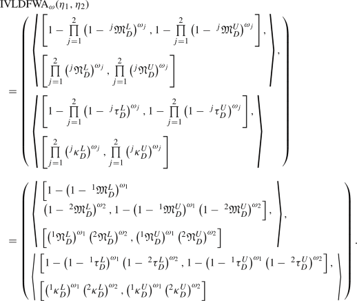
The aggregation value of IVLDFNs using the IVLDFWA operator is also an IVLDFN, and IVLDFWA$_{\omega }(\eta _{1},\eta _{2},...,\eta _{r})=$

(4.3)

(2):

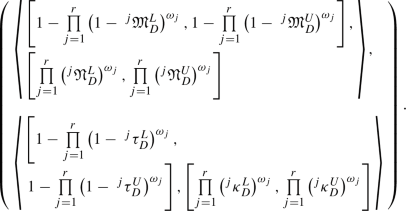
The aggregation value of IVLDFNs using the IVLDFWG operator is also an IVLDFN, and $IVLDFWG_{\omega }(\eta _{1},\eta _{2},...,\eta _{r})=$

(4.4)

Proof

(1):

Let us use the mathematical induction technique for proof. (i) For $r=1$, by Eq. (4.3), we write

(4.5)

Considering Definition 3.10 (c), we have

$$\begin{aligned} \omega _{1} \eta _{1} = \left( \begin{array}{l} \left\langle \begin{array}{l} \left[ 1-\left( 1-\ ^{1}{\mathfrak {M}}^{L}_{D}\right) ^{\omega _{1}},1-\left( 1-\ ^{1}{\mathfrak {M}}^{U}_{D}\right) ^{\omega _{1}}\right] , \left[ \left( ^{1}{\mathfrak {N}}^{L}_{D}\right) ^{\omega _{1}},\left( ^{1}{\mathfrak {N}}^{U}_{D}\right) ^{\omega _{1}}\right] \end{array} \right\rangle ,\\ \left\langle \begin{array}{l} \left[ 1-\left( 1-\ ^{1}\tau ^{L}_{D}\right) ^{\omega _{1}},1-\left( 1-\ ^{1}\tau ^{U}_{D}\right) ^{\omega _{1}}\right] , \left[ \left( ^{1}\kappa ^{L}_{D}\right) ^{\omega _{1}},\left( ^{1}\kappa ^{U}_{D}\right) ^{\omega _{1}}\right] \end{array} \right\rangle \end{array} \right) .\nonumber \\ \end{aligned}$$

(4.6)

Thus, by Eqs. (4.5) and (4.6), we have $IVLDFWA_{\omega }(\eta _{1})=\omega _{1} \eta _{1}$ and so Eq. (4.3) is valid for $r=1$. (ii) For $r=2$, by Eq. (4.3), we write

(4.7)

From Definition 3.10 (c), we can write

$$\begin{aligned} \omega _{1}\eta _{1}= \left( \begin{array}{l} \left\langle \left[ 1-\left( 1-\ ^{1}{\mathfrak {M}}^{L}_{\ddot{{\mathcal {D}}}}\right) ^{\omega _{1}},\ 1-\left( 1-\ ^{1}{\mathfrak {M}}^{U}_{\ddot{{\mathcal {D}}}}\right) ^{\omega _{1}}\right] , \ \left[ \left( ^{1}{\mathfrak {N}}^{L}_{\ddot{{\mathcal {D}}}}\right) ^{\omega _{1}},\ \left( ^{1}{\mathfrak {N}}^{U}_{\ddot{{\mathcal {D}}}}\right) ^{\omega _{1}}\right] \right\rangle ,\\ \left\langle \left[ 1-\left( 1-\ ^{1}\tau ^{L}_{\ddot{{\mathcal {D}}}}\right) ^{\omega _{1}},\ 1-\left( 1-\ ^{1}\tau ^{U}_{\ddot{{\mathcal {D}}}}\right) ^{\omega _{1}}\right] ,\ \left[ \left( ^{1}\kappa ^{U}_{\ddot{{\mathcal {D}}}}\right) ^{\omega _{1}},\ \left( ^{1}\kappa ^{U}_{\ddot{{\mathcal {D}}}}\right) ^{\omega _{1}}\right] \right\rangle \end{array} \right) \nonumber \\ \end{aligned}$$

(4.8)

and

$$\begin{aligned} \omega _{2}\eta _{2}= \left( \begin{array}{l} \left\langle \left[ 1-\left( 1-\ ^{2}{\mathfrak {M}}^{L}_{\ddot{{\mathcal {D}}}}\right) ^{\omega _{2}},\ 1-\left( 1-\ ^{2}{\mathfrak {M}}^{U}_{\ddot{{\mathcal {D}}}}\right) ^{\omega _{2}}\right] , \ \left[ \left( ^{2}{\mathfrak {N}}^{L}_{\ddot{{\mathcal {D}}}}\right) ^{\omega _{2}},\ \left( ^{2}{\mathfrak {N}}^{U}_{\ddot{{\mathcal {D}}}}\right) ^{\omega _{2}}\right] \right\rangle ,\\ \left\langle \left[ 1-\left( 1-\ ^{2}\tau ^{L}_{\ddot{{\mathcal {D}}}}\right) ^{\omega _{2}},\ 1-\left( 1-\ ^{2}\tau ^{U}_{\ddot{{\mathcal {D}}}}\right) ^{\omega _{2}}\right] ,\ \left[ \left( ^{2}\kappa ^{U}_{\ddot{{\mathcal {D}}}}\right) ^{\omega _{2}},\ \left( ^{2}\kappa ^{U}_{\ddot{{\mathcal {D}}}}\right) ^{\omega _{2}}\right] \right\rangle \end{array} \right) .\nonumber \\ \end{aligned}$$

(4.9)

By Definition 3.10 (a), the sum of $\omega _{1}\eta _{1}$ and $\omega _{2}\eta _{2}$ is calculated as follows: $\omega _{1}\eta _{1}\oplus \omega _{2}\eta _{2}=$

(4.10)

As a result of the calculations, it is seen that IVLDFWA$_{\omega }(\eta _{1},\eta _{2})= \omega _{1}\eta _{1}\oplus \omega _{2}\eta _{2}$. So, Eq. (4.3) is valid for $r=2$. (iii) If Eq. (4.3) holds for $r=k$, then we should demonstrate that Eq. (4.3) holds for $r=k+1$. That is, we must prove that IVLDFWA$_{\omega }(\eta _{1},\eta _{2},...,\eta _{k})\oplus \omega _{k+1}\eta _{k+1}=\textrm{IVLDFWA}_{\omega }(\eta _{1},\eta _{2},...,\eta _{k+1})$. Since Eq. (4.3) holds for $r=k$ and considering Definition 3.10 (a) and (c), we obtain IVLDFWA$_{\omega }(\eta _{1},\eta _{2},...,\eta _{k})\oplus \omega _{k+1}\eta _{k+1}=$

(4.11)

Then, we calculate as

$$\begin{aligned}{} & {} \!\!\!\!\!\left( 1-\prod \limits ^{k}_{j=1}\left( 1-\ ^{j}{\mathfrak {M}}^{L}_{D}\right) ^{\omega _{j}}\right) +\left( 1-\left( 1-\ ^{k+1}{\mathfrak {M}}^{L}_{\ddot{{\mathcal {D}}}}\right) ^{\omega _{k+1}}\right) \\{} & {} -\left( 1-\prod \limits ^{k}_{j=1}\left( 1-\ ^{j}{\mathfrak {M}}^{L}_{D}\right) ^{\omega _{j}}\right) \left( 1-\left( 1-\ ^{k+1}{\mathfrak {M}}^{L}_{\ddot{{\mathcal {D}}}}\right) ^{\omega _{k+1}}\right) =1-\prod \limits ^{k+1}_{j=1}\left( 1-\ ^{j}{\mathfrak {M}}^{L}_{D}\right) ^{\omega _{j}}, \end{aligned}$$

and $\left( \prod \limits ^{k}_{j=1}\left( \left( ^{j}\kappa ^{U}_{D}\right) ^{\omega _{j}}\right) \left( ^{k+1}\kappa ^{U}_{\ddot{{\mathcal {D}}}}\right) ^{\omega _{k+1}}\right) =\prod \limits ^{k+1}_{j=1}\left( ^{j}\kappa ^{U}_{D}\right) ^{\omega _{j}}$. Others can be calculated similarly. Thus, we have IVLDFWA$_{\omega }(\eta _{1},\eta _{2},...,\eta _{k})\oplus \omega _{k+1}\eta _{k+1}=$

(4.12)

So, if Eq. (4.3) is valid for $r=k$ then Eq. (4.3) is valid for $r=k+1$. Thus, the proof is completed.

(2):

It can be shown similarly to the proof of (1) using equations in Definition 3.10 (b) and (d).$\square$

4.2 An approach to MCDM based on supplier selection under IVLDF information

Let ${\mathfrak {X}}=\{x_{1},x_{2},...,x_{p}\}$ be a set of alternatives, ${\mathcal {E}}=\{\varepsilon _{1},\varepsilon _{2},...,\varepsilon _{r}\}$ be a set of criteria and its weight vector $\omega =\{\omega _{1},\omega _{2},...,\omega _{r}\}$ where $\omega _{j}\in [0,1]$ $(j=1,2,...,r)$ and $\sum \limits ^{r}_{j=1}\omega _{j}=1$. Let $\eta _{j}^{i}$ be the IVLDFN of the alternative $x_{i}$ with the respect to the criterion $\varepsilon _{j}$.

Algorithm 1. (Based on IVLDFWA and IVLDFWG)

• Step 1. Find the aggregation value $\eta ^{i}$ of LDFNs $\eta _{1}^{i}, \eta _{2}^{i},...,\eta _{r}^{i}$ using IVLDFWA operator or IVLDFWG operator, i.e., respectively

  $$\begin{aligned} \textrm{IVLDFWA}_{\omega }\left( \eta ^{i}_{1},\eta ^{i}_{2},...,\eta ^{i}_{r}\right) = \bigoplus \limits ^{r}_{j=1}\omega _{j}\eta ^{i}_{j}=\eta ^{i} \end{aligned}$$

  (4.13)

  or

  $$\begin{aligned} \textrm{IVLDFWG}_{\omega }\left( \eta ^{i}_{1},\eta ^{i}_{2},...,\eta ^{i}_{r}\right) = \bigotimes \limits ^{r}_{j=1}(\eta ^{i}_{j})^{\omega _{j}}=\eta ^{i}. \end{aligned}$$

  (4.14)

• Step 2. Calculate the values of score function $S(\eta ^{i})$ $\forall$ $i=1,2,\ldots , p$. If $S(\eta ^{i_{1}})=S(\eta ^{i_{2}})$ for any $i_{1},i_{2}\in \{1,2,\ldots , p\}$, then calculate the values of accuracy function $A(\eta ^{i_{1}})$ and $A(\eta ^{i_{2}})$ to rank $\eta ^{i_{1}}$ and $\eta ^{i_{2}}$.

• Step 3. Specify the optimal alternative according to the maximum value of score function $S(\eta ^{i})$ $(i=1,2,\ldots , p)$. (If there are two maximum values for the score function, then specify the optimal alternative according to the maximum value of the accuracy function).

Example 4.3

A high-technology manufacturing company desires to select a suitable material supplier to purchase the main components of new products. After preliminary screening, four candidates ($X=\{x_{1},x_{2},x_{3},x_{4}\}$) remain for further evaluation. A committee of decision makers has been formed to select the most suitable supplier. Three benefit criteria (parameters) are considered as “Technological Capability”, “Delivery Time”, and “Quality”. The weight vector of parameters is taken as $\omega =\{ 0.2, 0.5, 0.3\}$. Assume that “low cost” and “not low cost (or high cost)” are the reference parameters for the material suppliers. The hierarchical structure of this decision problem based on material supplier selection is shown in Fig. 3.

The tabular forms of interval-valued linear Diophantine fuzzy sets (IVLDFSs) corresponding to the given three criteria for the material suppliers are displayed in Tables 4, 5 and 6, respectively.

Fig. 3

Hierarchical structure of decision problem based on material supplier selection

Table 4 The table of IVLDFS for technological capability

Table 5 The table of IVLDFS for delivery time

Table 6 The table of IVLDFS for quality

We use the proposed aggregation operators IVLDFWA and IVLDFWG defined in Sect. 4 to pick out the suitable material supplier in keeping with Algorithm 1 as follows.

• Step 1. The aggregation value $\eta ^{i}$ of IVLDFNs $\eta _{1}^{i}, \eta _{2}^{i},...,\eta _{r}^{i}$ $(i=1,2,\ldots 4)$ are given in Table 7.

• Step 2. The score values $S(\eta ^{i})$ $(i=1,2,\ldots , p)$ and ranking order in keeping with the proposed aggregation operators IVLDFWA and IVLDFWG are displayed in Table 8.

• Step 3. We achieve the most suitable material supplier as $x_{3}$ in keeping with the proposed aggregation operators IVLDFWA and IVLDFWG from Table 8. Therefore, the material supplier with the high-end configurations and having a low cost is $x_{3}$. The comparison outcomes of each of the proposed aggregation operators IVLDFWA and IVLDFWG are visually displayed in Figure 4.

Table 7 The aggregation values of IVLDFWA and IVLDFWG operators

Table 8 The values of score function and ranking order

Fig. 4

Comparison outcomes of aggregation operators IVLDFWA and IVLDFWG

4.3 Comparative study for IVLDFWA and IVLDFWG

In this part, we examine our proposed aggregation operators Interval-Valued Linear Diophantine Fuzzy Weighted Average (IVLDFWA) and Interval-Valued Linear Diophantine Fuzzy Weighted Geometric (IVLDFWG) with some existing operators GIVIFIWA (Garg 2016a), O-PFWPA, O-PFWPG (Yager 2014), PFOWA, PFOWG (Xu et al. 2017), IVPFWHM, IVPFWDHM (Li et al. 2018), IVPFWA, IVPFWG (Garg 2016b), q-ROFHWAGA (Riaz et al. 2020a), q-ROFWA, q-ROFWG (Liu and Wang 2018), Algebraic, Einstein, Hamacher, Frank (Gao et al. 2019), SF, ESF (Riaz and Hashmi 2019) based on the existing models IVIFS, PyFS, IVPyFS, q-ROFS, IVq-ROFS, and LDFS. The comparison effects are provided in Table 9.

Table 9 Comparison of proposed operators (IVLDFWA and IVLDFWG) with existing operators

Advantages of proposed IVLDFWA and IVLDFWG aggregation operators

Any IFN $(\langle {\mathfrak {M}}_{{\mathcal {I}}},{\mathfrak {N}}_{{\mathcal {I}}}\rangle )$ may be considered as IVLDFN $(\langle [{\mathfrak {M}}_{{\mathcal {I}}},{\mathfrak {M}}_{{\mathcal {I}}}],[{\mathfrak {N}}_{{\mathcal {I}}},{\mathfrak {N}}_{{\mathcal {I}}}]\rangle , \langle [0,0],[0,0]\rangle )$. (For instance, $(\langle 0.7,0.2\rangle )$ corresponds to $(\langle [0.7,0.7],[0.2,0.2]\rangle , \langle [0,0],[0,0]\rangle )$ ). Using the matching of the existing notions IVIFN, PyFN, IVPyFN, q-ROFN, IVq-ROFN, and LDFN with the proposed IVLDFN, one can utilize our proposed aggregation operators IVLDFWA and IVLDFWG to solve the MCDM problems under the environment of IVIFS, PyFS, IVPyFS, q-ROFS, IVq-ROFS, and LDFS. However, the existing operators GIVIFIWA (Garg 2016a), O-PFWPA, O-PFWPG (Yager 2014), PFOWA, PFOWG (Xu et al. 2017), IVPFWHM, IVPFWDHM (Li et al. 2018), IVPFWA, IVPFWG (Garg 2016b), q-ROFHWAGA (Riaz et al. 2020a), q-ROFWA, q-ROFWG (Liu and Wang 2018), Algebraic, Einstein, Hamacher, Frank (Gao et al. 2019), SF, ESF (Riaz and Hashmi 2019) based on the existing notions IVIFS, PyFS, IVPyFS, q-ROFS, IVq-ROFS, and LDFS can not be utilized to solve the MCDM problems where data is collected under IVLDF information. It suggests that our proposed aggregation operators IVLDFWA and IVLDFWG are advanced than the existing aggregation operators mentioned in Garg (2016a, 2016b), Xu et al. (2017), Yager (2014), Li et al. (2018), Riaz and Hashmi (2019), Riaz et al. (2020a), Liu and Wang (2018), Gao et al. (2019).

5 Correlation coefficients for IVLDFSs and their application in medical diagnosis

In this section, we describe some correlation coefficients for the IVLDFSs and they applied in medical diagnosis.

5.1 Correlation coefficients for IVLDFSs

Let

$\ddot{{\mathcal {D}}}_{1}$=$\left\{ \left( x_{i},\left\langle \left[ {\mathfrak {M}}^{L}_{\ddot{{\mathcal {D}}}_{1}}(x_{i}),{\mathfrak {M}}^{U}_{\ddot{{\mathcal {D}}}_{1}}(x_{i})\right] , \left[ {\mathfrak {N}}^{L}_{\ddot{{\mathcal {D}}}_{1}}(x_{i}),{\mathfrak {N}}^{U}_{\ddot{{\mathcal {D}}}_{1}}(x_{i})\right] \right\rangle , \left\langle \left[ ^{(i)}\tau ^{L}_{\ddot{{\mathcal {D}}}_{1}},^{(i)}\tau ^{U}_{\ddot{{\mathcal {D}}}_{1}}\right] , \left[ ^{(i)}\kappa ^{L}_{\ddot{{\mathcal {D}}}_{1}},^{(i)}\kappa ^{U}_{\ddot{{\mathcal {D}}}_{1}}\right] \right\rangle \right) : x_{i}\in {\mathfrak {X}}\right\}$

and

$\ddot{{\mathcal {D}}}_{2}$=$\left\{ \left( x_{i},\left\langle \left[ {\mathfrak {M}}^{L}_{\ddot{{\mathcal {D}}}_{2}}(x_{i}),{\mathfrak {M}}^{U}_{\ddot{{\mathcal {D}}}_{2}}(x_{i})\right] , \left[ {\mathfrak {N}}^{L}_{\ddot{{\mathcal {D}}}_{2}}(x_{i}),{\mathfrak {N}}^{U}_{\ddot{{\mathcal {D}}}_{2}}(x_{i})\right] \right\rangle ,\right. \right.$ $\left. \left. \left\langle \left[ ^{(i)}\tau ^{L}_{\ddot{{\mathcal {D}}}_{2}},^{(i)}\tau ^{U}_{\ddot{{\mathcal {D}}}_{2}}\right] , \left[ ^{(i)}\kappa ^{L}_{\ddot{{\mathcal {D}}}_{2}},^{(i)}\kappa ^{U}_{\ddot{{\mathcal {D}}}_{2}}\right] \right\rangle \right) : x_{i}\in {\mathfrak {X}}\right\}$

be two IVLDFSs over the universal discourse set ${\mathfrak {X}}=\{x_{1},x_{2},...,x_{p}\}$. Then, the informational energies of two IVLDFSs $\ddot{{\mathcal {D}}}_{1}$ and $\ddot{{\mathcal {D}}}_{2}$ are described as

$$\begin{aligned} T\left( \ddot{{\mathcal {D}}}_{1}\right)= & {} \sum \limits ^{p}_{i=1}\left( \left( {\mathfrak {M}}^{L}_{\ddot{{\mathcal {D}}}_{1}}(x_{i})\right) ^{2}+\left( {\mathfrak {M}}^{U}_{\ddot{{\mathcal {D}}}_{1}}(x_{i})\right) ^{2}\right. \nonumber \\{} & {} \left. +\left( {\mathfrak {N}}^{L}_{\ddot{{\mathcal {D}}}_{1}}(x_{i})\right) ^{2}+\left( {\mathfrak {N}}^{U}_{\ddot{{\mathcal {D}}}_{1}}(x_{i})\right) ^{2}+\left( ^{(i)}\tau ^{L}_{\ddot{{\mathcal {D}}}_{1}}\right) ^{2}+\left( ^{(i)}\tau ^{U}_{\ddot{{\mathcal {D}}}_{1}}\right) ^{2}\right. \nonumber \\{} & {} \left. +\,\left( ^{(i)}\kappa ^{L}_{\ddot{{\mathcal {D}}}_{1}}\right) ^{2}+\left( ^{(i)}\kappa ^{U}_{\ddot{{\mathcal {D}}}_{1}}\right) ^{2}\right) , \end{aligned}$$

(5.1)

$$\begin{aligned} T\left( \ddot{{\mathcal {D}}}_{2}\right)= & {} \sum \limits ^{p}_{i=1}\left( \left( {\mathfrak {M}}^{L}_{\ddot{{\mathcal {D}}}_{2}}(x_{i})\right) ^{2}+\left( {\mathfrak {M}}^{U}_{\ddot{{\mathcal {D}}}_{2}}(x_{i})\right) ^{2}+\left( {\mathfrak {N}}^{L}_{\ddot{{\mathcal {D}}}_{2}}(x_{i})\right) ^{2}+\left( {\mathfrak {N}}^{U}_{\ddot{{\mathcal {D}}}_{2}}(x_{i})\right) ^{2}+\left( ^{(i)}\tau ^{L}_{\ddot{{\mathcal {D}}}_{2}}\right) ^{2}\right. \nonumber \\{} & {} \left. +\left( ^{(i)}\tau ^{U}_{\ddot{{\mathcal {D}}}_{2}}\right) ^{2}+\left( ^{(i)}\kappa ^{L}_{\ddot{{\mathcal {D}}}_{2}}\right) ^{2}+\left( ^{(i)}\kappa ^{U}_{\ddot{{\mathcal {D}}}_{2}}\right) ^{2}\right) . \end{aligned}$$

(5.2)

The correlation of the IVLDFSs $\ddot{{\mathcal {D}}}_{1}$ and $\ddot{{\mathcal {D}}}_{2}$ is defined as

$$\begin{aligned}{} & {} C\left( \ddot{{\mathcal {D}}}_{1},\ddot{{\mathcal {D}}}_{2}\right) \nonumber \\ {}{} & {} =\sum \limits ^{p}_{i=1} \left( \begin{array}{l} {\mathfrak {M}}^{L}_{\ddot{{\mathcal {D}}}_{1}}(x_{i}){\mathfrak {M}}^{L}_{\ddot{{\mathcal {D}}}_{2}}(x_{i})+{\mathfrak {M}}^{U}_{\ddot{{\mathcal {D}}}_{1}}(x_{i}){\mathfrak {M}}^{U}_{\ddot{{\mathcal {D}}}_{2}}(x_{i})+ {\mathfrak {N}}^{L}_{\ddot{{\mathcal {D}}}_{1}}(x_{i}){\mathfrak {N}}^{L}_{\ddot{{\mathcal {D}}}_{2}}(x_{i})+{\mathfrak {N}}^{U}_{\ddot{{\mathcal {D}}}_{1}}(x_{i}){\mathfrak {N}}^{U}_{\ddot{{\mathcal {D}}}_{2}}(x_{i})\\ + ^{(i)}\tau ^{L}_{\ddot{{\mathcal {D}}}_{1}}\ ^{(i)}\tau ^{L}_{\ddot{{\mathcal {D}}}_{2}}+\ ^{(i)}\tau ^{U}_{\ddot{{\mathcal {D}}}_{1}}\ ^{(i)}\tau ^{U}_{\ddot{{\mathcal {D}}}_{2}}+\ ^{(i)}\kappa ^{L}_{\ddot{{\mathcal {D}}}_{1}}\ ^{(i)}\kappa ^{L}_{\ddot{{\mathcal {D}}}_{2}}+^{(i)}\kappa ^{U}_{\ddot{{\mathcal {D}}}_{1}}\ ^{(i)}\kappa ^{U}_{\ddot{{\mathcal {D}}}_{2}} \end{array} \right) . \end{aligned}$$

(5.3)

It can be easily verified from Eq. (5.1) and Eq. (5.3) that the correlation of IVLDFSs satisfies the following properties:

• $C\left( \ddot{{\mathcal {D}}}_{1},\ddot{{\mathcal {D}}}_{2}\right) =C\left( \ddot{{\mathcal {D}}}_{2},\ddot{{\mathcal {D}}}_{1}\right)$.

• $C\left( \ddot{{\mathcal {D}}}_{1},\ddot{{\mathcal {D}}}_{1}\right) =T(\ddot{{\mathcal {D}}}_{1})$.

Now, based on these concepts, we propose the correlation coefficients between IVLDFSs

Definition 5.1

Let $\ddot{{\mathcal {D}}}_{1}$ and $\ddot{{\mathcal {D}}}_{2}$ be two IVLDFSs over the universal discourse set ${\mathfrak {X}}=\{x_{1},x_{2},...,x_{p}\}$.

(a):

The type-1 correlation coefficient (type-1 CoCo) between $\ddot{{\mathcal {D}}}_{1}$ and $\ddot{{\mathcal {D}}}_{2}$ is denoted by ${\mathfrak {C}}^{1}(\ddot{{\mathcal {D}}}_{1},\ddot{{\mathcal {D}}}_{2})$ and defined as

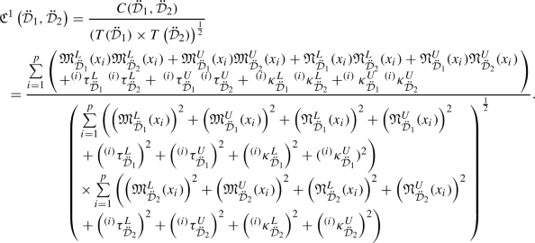(5.4)

(b):

The type-2 correlation coefficient (type-2 CoCo) between $\ddot{{\mathcal {D}}}_{1}$ and $\ddot{{\mathcal {D}}}_{2}$ is denoted by ${\mathfrak {C}}^{2}(\ddot{{\mathcal {D}}}_{1},\ddot{{\mathcal {D}}}_{2})$ and defined as

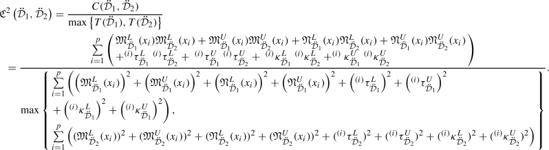(5.5)

Theorem 5.2

The correlation coefficients (CoCos) between two IVLDFSs $\ddot{{\mathcal {D}}}_{1}$ and $\ddot{{\mathcal {D}}}_{2}$, as defined in Eq. (5.4) and Eq. (5.5), satisfies the following properties. For $t=1,2$,

(1):

$0 \le {\mathfrak {C}}^{t}(\ddot{{\mathcal {D}}}_{1},\ddot{{\mathcal {D}}}_{2})\le 1$.

(2):

${\mathfrak {C}}^{t}(\ddot{{\mathcal {D}}}_{1},\ddot{{\mathcal {D}}}_{2})={\mathfrak {C}}^{t}(\ddot{{\mathcal {D}}}_{2},\ddot{{\mathcal {D}}}_{1})$.

(3):

${\mathfrak {C}}^{t}(\ddot{{\mathcal {D}}}_{1},\ddot{{\mathcal {D}}}_{2})=1$ if $\ddot{{\mathcal {D}}}_{1}=\ddot{{\mathcal {D}}}_{2}$.

Proof

Let us verify the above properties for $t=1$. It can be verified in a similar way for $t=2$.

(1):

Since ${\mathfrak {M}}_{\ddot{{\mathcal {D}}}_{1}}(x_{i})$,${\mathfrak {M}}_{\ddot{{\mathcal {D}}}_{2}}(x_{i})$, ${\mathfrak {N}}_{\ddot{{\mathcal {D}}}_{1}}(x_{i})$, ${\mathfrak {N}}_{\ddot{{\mathcal {D}}}_{2}}(x_{i})$,$^{(i)}\tau _{\ddot{{\mathcal {D}}}_{1}}$, $^{(i)}\tau _{\ddot{{\mathcal {D}}}_{2}}$,$^{(i)}\kappa _{\ddot{{\mathcal {D}}}_{1}}$,$^{(i)}\kappa _{\ddot{{\mathcal {D}}}_{2}}\in {\mathfrak {I}}^{[0,1]}$ for all $x_{i}\in {\mathfrak {X}}$, we have $C(\ddot{{\mathcal {D}}}_{1},\ddot{{\mathcal {D}}}_{2})\ge 0$, $T(\ddot{{\mathcal {D}}}_{1})\ge 0$ and $T(\ddot{{\mathcal {D}}}_{2})\ge 0$. So, we obtain ${\mathfrak {C}}^{1}(\ddot{{\mathcal {D}}}_{1},\ddot{{\mathcal {D}}}_{2})\ge 0$. Now, we shall prove ${\mathfrak {C}}^{1}(\ddot{{\mathcal {D}}}_{1},\ddot{{\mathcal {D}}}_{2})\le 1$.

By Eq. (5.4), we write

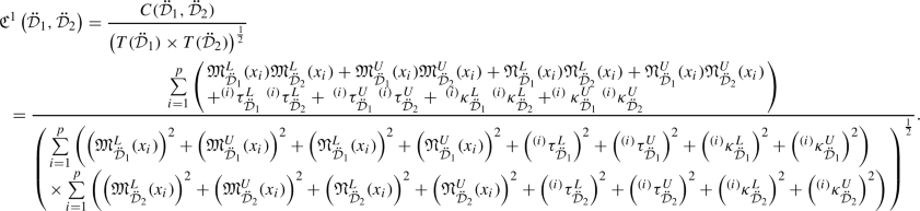(5.6)

Using Cauchy–Schwarz inequality (i.e., $(\sum \nolimits ^{p}_{i=1}u_{i}v_{i})^{2}\le (\sum \nolimits ^{p}_{i=1}u^{2}_{i})(\sum \nolimits ^{p}_{i=1}v^{2}_{i})$), we have ${\mathfrak {C}}^{1}(\ddot{{\mathcal {D}}}_{1},\ddot{{\mathcal {D}}}_{2})\le$

$$\begin{aligned} \frac{ \left( \begin{array}{l} \left( \sum \limits ^{p}_{i=1}\left( {\mathfrak {M}}^{L}_{\ddot{{\mathcal {D}}}_{1}}(x_{i})\right) ^{2}\right) ^{\frac{1}{2}}\left( \sum \limits ^{p}_{i=1}\left( {\mathfrak {M}}^{L}_{\ddot{{\mathcal {D}}}_{2}}(x_{i})\right) ^{2}\right) ^{\frac{1}{2}}+ \left( \sum \limits ^{p}_{i=1}\left( {\mathfrak {M}}^{U}_{\ddot{{\mathcal {D}}}_{1}}(x_{i})\right) ^{2}\right) ^{\frac{1}{2}}\left( \sum \limits ^{p}_{i=1}\left( {\mathfrak {M}}^{U}_{\ddot{{\mathcal {D}}}_{2}}(x_{i})\right) ^{2}\right) ^{\frac{1}{2}} \\ + \left( \sum \limits ^{p}_{i=1}\left( {\mathfrak {N}}^{L}_{\ddot{{\mathcal {D}}}_{1}}(x_{i})\right) ^{2}\right) ^{\frac{1}{2}}\left( \sum \limits ^{p}_{i=1}\left( {\mathfrak {N}}^{L}_{\ddot{{\mathcal {D}}}_{2}}(x_{i})\right) ^{2}\right) ^{\frac{1}{2}}+ \left( \sum \limits ^{p}_{i=1}\left( {\mathfrak {N}}^{U}_{\ddot{{\mathcal {D}}}_{1}}(x_{i})\right) ^{2}\right) ^{\frac{1}{2}}\left( \sum \limits ^{p}_{i=1}\left( {\mathfrak {N}}^{U}_{\ddot{{\mathcal {D}}}_{2}}(x_{i})\right) ^{2}\right) ^{\frac{1}{2}}\\ + \left( \sum \limits ^{p}_{i=1}\left( ^{(i)}\tau ^{L}_{\ddot{{\mathcal {D}}}_{1}}\right) ^{2}\right) ^{\frac{1}{2}}\ \left( \sum \limits ^{p}_{i=1}\left( ^{(i)}\tau ^{L}_{\ddot{{\mathcal {D}}}_{2}}\right) ^{2}\right) ^{\frac{1}{2}}+ \left( \sum \limits ^{p}_{i=1}\left( ^{(i)}\tau ^{U}_{\ddot{{\mathcal {D}}}_{1}}\right) ^{2}\right) ^{\frac{1}{2}} \left( \sum \limits ^{p}_{i=1}\left( ^{(i)}\tau ^{U}_{\ddot{{\mathcal {D}}}_{2}}\right) ^{2}\right) ^{\frac{1}{2}}\\ + \left( \sum \limits ^{p}_{i=1}\left( ^{(i)}\kappa ^{L}_{\ddot{{\mathcal {D}}}_{1}}\right) ^{2}\right) ^{\frac{1}{2}} \left( \sum \limits ^{p}_{i=1}\left( ^{(i)}\kappa ^{L}_{\ddot{{\mathcal {D}}}_{2}}\right) ^{2}\right) ^{\frac{1}{2}}+ \left( \sum \limits ^{p}_{i=1}\left( ^{(i)}\kappa ^{U}_{\ddot{{\mathcal {D}}}_{1}}\right) ^{2}\right) ^{\frac{1}{2}} \left( \sum \limits ^{p}_{i=1}\left( ^{(i)}\kappa ^{U}_{\ddot{{\mathcal {D}}}_{2}}\right) ^{2}\right) ^{\frac{1}{2}} \end{array} \right) }{ \left( \begin{array}{l} \sum \limits ^{p}_{i=1}\big (({\mathfrak {M}}^{L}_{\ddot{{\mathcal {D}}}_{1}}(x_{i}))^{2}+({\mathfrak {M}}^{U}_{\ddot{{\mathcal {D}}}_{1}}(x_{i}))^{2}+({\mathfrak {N}}^{L}_{\ddot{{\mathcal {D}}}_{1}}(x_{i}))^{2}+({\mathfrak {N}}^{U}_{\ddot{{\mathcal {D}}}_{1}}(x_{i}))^{2}+(^{(i)}\tau ^{L}_{\ddot{{\mathcal {D}}}_{1}})^{2}+(^{(i)}\tau ^{U}_{\ddot{{\mathcal {D}}}_{1}})^{2}+(^{(i)}\kappa ^{L}_{\ddot{{\mathcal {D}}}_{1}})^{2}+(^{(i)}\kappa ^{U}_{\ddot{{\mathcal {D}}}_{1}})^{2}\big ) \\ \times \sum \limits ^{p}_{i=1}\left( \left( {\mathfrak {M}}^{L}_{\ddot{{\mathcal {D}}}_{2}}(x_{i})\right) ^{2}+\left( {\mathfrak {M}}^{U}_{\ddot{{\mathcal {D}}}_{2}}(x_{i})\right) ^{2}+\left( {\mathfrak {N}}^{L}_{\ddot{{\mathcal {D}}}_{2}}(x_{i})\right) ^{2}+\left( {\mathfrak {N}}^{U}_{\ddot{{\mathcal {D}}}_{2}}(x_{i})\right) ^{2}+\left( ^{(i)}\tau ^{L}_{\ddot{{\mathcal {D}}}_{2}}\right) ^{2}+\left( ^{(i)}\tau ^{U}_{\ddot{{\mathcal {D}}}_{2}}\right) ^{2}+\left( ^{(i)}\kappa ^{L}_{\ddot{{\mathcal {D}}}_{2}}\right) ^{2}+\left( ^{(i)}\kappa ^{U}_{\ddot{{\mathcal {D}}}_{2}}\right) ^{2}\right) \end{array} \right) ^{\frac{1}{2}}}.\nonumber \\ \end{aligned}$$

(5.7)

If we take the following notations

$$\begin{aligned} \left\{ {\begin{array}{ll} \sum \limits ^{p}_{i=1}\left( {\mathfrak {M}}^{L}_{\ddot{{\mathcal {D}}}_{1}}(x_{i})\right) ^{2}=a_{1},\ \sum \limits ^{p}_{i=1}\left( {\mathfrak {M}}^{L}_{\ddot{{\mathcal {D}}}_{2}}(x_{i})\right) ^{2}=a_{2},\ \sum \limits ^{p}_{i=1}\left( {\mathfrak {M}}^{U}_{\ddot{{\mathcal {D}}}_{1}}(x_{i})\right) ^{2}=b_{1},\ \sum \limits ^{p}_{i=1}\left( {\mathfrak {M}}^{U}_{\ddot{{\mathcal {D}}}_{2}}(x_{i})\right) ^{2}=b_{2},\\ \sum \limits ^{p}_{i=1}\left( {\mathfrak {N}}^{L}_{\ddot{{\mathcal {D}}}_{1}}(x_{i})\right) ^{2}=c_{1},\ \sum \limits ^{p}_{i=1}\left( {\mathfrak {N}}^{L}_{\ddot{{\mathcal {D}}}_{2}}(x_{i})\right) ^{2}=c_{2},\ \sum \limits ^{p}_{i=1}\left( {\mathfrak {N}}^{U}_{\ddot{{\mathcal {D}}}_{1}}(x_{i})\right) ^{2}=d_{1},\ \sum \limits ^{p}_{i=1}\left( {\mathfrak {N}}^{U}_{\ddot{{\mathcal {D}}}_{2}}(x_{i})\right) ^{2}=d_{2},\\ \sum \limits ^{p}_{i=1}\left( ^{(i)}\tau ^{L}_{\ddot{{\mathcal {D}}}_{1}}\right) ^{2}=e_{1},\ \sum \limits ^{p}_{i=1}\left( ^{(i)}\tau ^{L}_{\ddot{{\mathcal {D}}}_{2}}\right) ^{2}=e_{2},\ \sum \limits ^{p}_{i=1}\left( ^{(i)}\tau ^{U}_{\ddot{{\mathcal {D}}}_{1}}\right) ^{2}=f_{1},\ \sum \limits ^{p}_{i=1}\left( ^{(i)}\tau ^{U}_{\ddot{{\mathcal {D}}}_{2}}\right) ^{2}=f_{2},\\ \sum \limits ^{p}_{i=1}\left( ^{(i)}\kappa ^{L}_{\ddot{{\mathcal {D}}}_{1}}\right) ^{2}=g_{1},\ \sum \limits ^{p}_{i=1}\left( ^{(i)}\kappa ^{L}_{\ddot{{\mathcal {D}}}_{2}}\right) ^{2}=g_{2},\ \sum \limits ^{p}_{i=1}\left( ^{(i)}\kappa ^{U}_{\ddot{{\mathcal {D}}}_{1}}\right) ^{2}=h_{1},\ \sum \limits ^{p}_{i=1}\left( ^{(i)}\kappa ^{U}_{\ddot{{\mathcal {D}}}_{2}}\right) ^{2}=h_{2}, \end{array}} \right\} , \end{aligned}$$

then Eq. (5.7) reduces to

$$\begin{aligned}{} & {} {\mathfrak {C}}^{1}\left( \ddot{{\mathcal {D}}}_{1},\ddot{{\mathcal {D}}}_{2}\right) \nonumber \\{} & {} \quad \le \frac{ \left( \sqrt{a_{1}a_{2}}+\sqrt{b_{1}b_{2}}+\sqrt{c_{1}c_{2}}+\sqrt{d_{1}d_{2}}+\sqrt{e_{1}e_{2}}+\sqrt{f_{1}f_{2}}+\sqrt{g_{1}g_{2}}+\sqrt{h_{1}h_{2}}\right) }{ \sqrt{\left( a_{1}+b_{1}+c_{1}+d_{1}+e_{1}+f_{1}+g_{1}+h_{1}\right) \times \left( a_{1}+b_{1}+c_{1}+d_{1}+e_{1}+f_{1}+g_{1}+h_{1}\right) }}.\nonumber \\ \end{aligned}$$

(5.8)

Then, we calculate

$$\begin{aligned}{} & {} \left( {\mathfrak {C}}^{1}(\ddot{{\mathcal {D}}}_{1},\ddot{{\mathcal {D}}}_{2})\right) ^{2}\nonumber \\{} & {} \le \frac{\left( \left( \sqrt{a_{1}a_{2}}+\sqrt{b_{1}b_{2}}+\sqrt{c_{1}c_{2}}+\sqrt{d_{1}d_{2}}+\sqrt{e_{1}e_{2}}+\sqrt{f_{1}f_{2}}+\sqrt{g_{1}g_{2}}+\sqrt{h_{1}h_{2}}\right) \right) ^{2}}{ (a_{1}+b_{1}+c_{1}+d_{1}+e_{1}+f_{1}+g_{1}+h_{1})\times (a_{1}+b_{1}+c_{1}+d_{1}+e_{1}+f_{1}+g_{1}+h_{1})}\nonumber \\{} & {} \quad =\frac{\left( \begin{array}{l} a_{1}a_{2}+b_{1}b_{2}+c_{1}c_{2}+d_{1}d_{2}+e_{1}e_{2}+f_{1}f_{2}+g_{1}g_{2}+h_{1}h_{2} \\ +2\sqrt{a_{1}a_{2}}\sqrt{b_{1}b_{2}} +2\sqrt{a_{1}a_{2}}\sqrt{c_{1}c_{2}} +2\sqrt{a_{1}a_{2}}\sqrt{d_{1}d_{2}}+2\sqrt{a_{1}a_{2}}\sqrt{e_{1}e_{2}}\\ +2\sqrt{a_{1}a_{2}}\sqrt{f_{1}f_{2}} +2\sqrt{a_{1}a_{2}}\sqrt{g_{1}g_{2}}+2\sqrt{a_{1}a_{2}}\sqrt{h_{1}h_{2}} +2\sqrt{b_{1}b_{2}}\sqrt{c_{1}c_{2}}\\ +2\sqrt{b_{1}b_{2}}\sqrt{d_{1}d_{2}} +2\sqrt{b_{1}b_{2}}\sqrt{e_{1}e_{2}}+2\sqrt{b_{1}b_{2}}\sqrt{f_{1}f_{2}}+2\sqrt{b_{1}b_{2}}\sqrt{g_{1}g_{2}} \\ +2\sqrt{b_{1}b_{2}}\sqrt{h_{1}h_{2}} +2\sqrt{c_{1}c_{2}}\sqrt{d_{1}d_{2}}+2\sqrt{c_{1}c_{2}}\sqrt{e_{1}e_{2}}+2\sqrt{c_{1}c_{2}}\sqrt{f_{1}f_{2}}\\ +2\sqrt{c_{1}c_{2}}\sqrt{g_{1}g_{2}} +2\sqrt{c_{1}c_{2}}\sqrt{h_{1}h_{2}} +2\sqrt{d_{1}d_{2}}\sqrt{e_{1}e_{2}}+2\sqrt{d_{1}d_{2}}\sqrt{f_{1}f_{2}}\\ +2\sqrt{d_{1}d_{2}}\sqrt{g_{1}g_{2}} +2\sqrt{d_{1}d_{2}}\sqrt{h_{1}h_{2}} +2\sqrt{e_{1}e_{2}}\sqrt{f_{1}f_{2}}+2\sqrt{e_{1}e_{2}}\sqrt{g_{1}g_{2}}\\ +2\sqrt{e_{1}e_{2}}\sqrt{h_{1}h_{2}} +2\sqrt{f_{1}f_{2}}\sqrt{g_{1}g_{2}}+2\sqrt{f_{1}f_{2}}\sqrt{h_{1}h_{2}} +2\sqrt{f_{1}f_{2}}\sqrt{h_{1}h_{2}} \end{array} \right) }{\left( \begin{array}{l} a_{1}a_{2}+b_{1}b_{2}+c_{1}c_{2}+d_{1}d_{2}+e_{1}e_{2}+f_{1}f_{2}+g_{1}g_{2}+h_{1}h_{2} +a_{1}b_{2}+a_{1}c_{2}+a_{1}d_{2}\\ +a_{1}e_{2}+a_{1}f_{2} +a_{1}g_{2} +a_{1}h_{2} +b_{1}a_{2}+b_{1}c_{2}+b_{1}d_{2}+b_{1}e_{2}+b_{1}f_{2}\\ +b_{1}g_{2}+b_{1}h_{2} +c_{1}a_{2}+c_{1}b_{2}+c_{1}d_{2}+c_{1}e_{2}\\ +c_{1}f_{2}+c_{1}g_{2} +c_{1}h_{2} +d_{1}a_{2}+d_{1}b_{2}+d_{1}c_{2}+d_{1}e_{2}\\ +d_{1}f_{2}+d_{1}g_{2}+d_{1}h_{2} +e_{1}a_{2}+e_{1}b_{2}+e_{1}c_{2}\\ +e_{1}d_{2} +e_{1}f_{2}+e_{1}g_{2} +e_{1}h_{2} +f_{1}a_{2}+f_{1}b_{2}+f_{1}c_{2}+f_{1}d_{2}\\ +f_{1}e_{2}+f_{1}g_{2}+f_{1}h_{2} +g_{1}a_{2} +g_{1}b_{2}\\ +g_{1}c_{2}+g_{1}d_{2}+g_{1}e_{2}+g_{1}f_{2} +g_{1}h_{2} +h_{1}a_{2}+h_{1}b_{2}+h_{1}c_{2}\\ +h_{1}d_{2}+h_{1}e_{2}+h_{1}f_{2}+h_{1}g_{2} \end{array} \right) }.\nonumber \\ \end{aligned}$$

(5.9)

For the positive numbers $\gamma _{1},\gamma _{2}, \delta _{1}, \delta _{2}$, we have $(\sqrt{\gamma _{1}\delta _{2}}-\sqrt{\delta _{1}\gamma _{2}})^{2}\ge 0$. Then, we obtain $\gamma _{1}\delta _{2}+\delta _{1}\gamma _{2}-2\sqrt{\gamma _{1}\delta _{2}}\sqrt{\delta _{1}\gamma _{2}}\ge 0$ and so

$$\begin{aligned} \gamma _{1}\delta _{2}+\delta _{1}\gamma _{2}\ge 2\sqrt{\gamma _{1}\delta _{2}}\sqrt{\delta _{1}\gamma _{2}}. \end{aligned}$$

(5.10)

Considering Eq. (5.10), we have $\big ({\mathfrak {C}}^{1}(\ddot{{\mathcal {D}}}_{1},\ddot{{\mathcal {D}}}_{2})\big )^{2}\le 1$ and thus ${\mathfrak {C}}^{1}(\ddot{{\mathcal {D}}}_{1},\ddot{{\mathcal {D}}}_{2})\le 1$. Thus, we prove that $0\le {\mathfrak {C}}^{1}(\ddot{{\mathcal {D}}}_{1},\ddot{{\mathcal {D}}}_{2})\le 1$.

(2):

It is obvious that ${\mathfrak {C}}^{1}(\ddot{{\mathcal {D}}}_{1},\ddot{{\mathcal {D}}}_{2})={\mathfrak {C}}^{1}(\ddot{{\mathcal {D}}}_{2},\ddot{{\mathcal {D}}}_{1})$ due to $C(\ddot{{\mathcal {D}}}_{1},\ddot{{\mathcal {D}}}_{2})=C(\ddot{{\mathcal {D}}}_{2},\ddot{{\mathcal {D}}}_{1})$ and $T(\ddot{{\mathcal {D}}}_{1})\times T(\ddot{{\mathcal {D}}}_{2})=T(\ddot{{\mathcal {D}}}_{2})\times T(\ddot{{\mathcal {D}}}_{1})$.

(3):

If $\ddot{{\mathcal {D}}}_{1}=\ddot{{\mathcal {D}}}_{2}$ then $C(\ddot{{\mathcal {D}}}_{1},\ddot{{\mathcal {D}}}_{1})=T(\ddot{{\mathcal {D}}}_{1})$ and hence

$$\begin{aligned} {\mathfrak {C}}^{1}\left( \ddot{{\mathcal {D}}}_{1},\ddot{{\mathcal {D}}}_{1}\right) =\frac{C\left( \ddot{{\mathcal {D}}}_{1},\ddot{{\mathcal {D}}}_{1}\right) }{\left( T(\ddot{{\mathcal {D}}}_{1})\times T(\ddot{{\mathcal {D}}}_{1})\right) ^{\frac{1}{2}}}=\frac{T(\ddot{{\mathcal {D}}}_{1})}{\left( \left( T\left( \ddot{{\mathcal {D}}}_{1}\right) \right) ^{2}\right) ^{\frac{1}{2}}}=1. \end{aligned}$$

(5.11)

$\square$

In real-life situations, sometimes, we must take into account the proper weightage dedicated to some elements. Therefore, we propose weighted correlation coefficients for IVLDFSs in the following definition.

Definition 5.3

Let $\ddot{{\mathcal {D}}}_{1}$ and $\ddot{{\mathcal {D}}}_{2}$ be two IVLDFSs over the universal discourse set ${\mathfrak {X}}=\{x_{1},x_{2},...,x_{p}\}$. Also, let $\omega =(\omega _{1},\omega _{2},...,\omega _{p})^{T}$ be the weighted vector corresponding to the elements $x_{i}$ $(i=1,2,...,p)$ with $\omega _{i}\in [0,1]$ and $\sum \limits ^{p}_{i=1}\omega _{i}=1$.

(a):

The type-1 weighted correlation coefficient (type-1 WCoCo) between $\ddot{{\mathcal {D}}}_{1}$ and $\ddot{{\mathcal {D}}}_{2}$ is denoted by ${\mathfrak {C}}^{1}_{\omega }(\ddot{{\mathcal {D}}}_{1},\ddot{{\mathcal {D}}}_{2})$and defined as

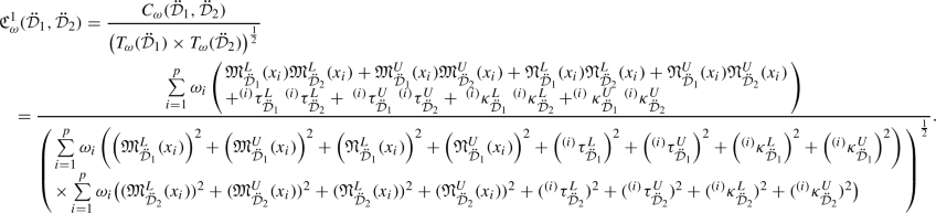(5.12)

(b):

The type-2 weighted correlation coefficient (type-2 WCoCo) between $\ddot{{\mathcal {D}}}_{1}$ and $\ddot{{\mathcal {D}}}_{2}$ is denoted by ${\mathfrak {C}}^{2}_{\omega }(\ddot{{\mathcal {D}}}_{1},\ddot{{\mathcal {D}}}_{2})$ and defined as

(5.13)

Fig. 5

The symptoms of COVID-19, influenza, cold (Source: World Health Organization (WHO))

Table 10 The table of IVLDFS for patient $\wp$

Theorem 5.4

The weighted correlation coefficients (WCoCos) between two IVLDFSs $\ddot{{\mathcal {D}}}_{1}$ and $\ddot{{\mathcal {D}}}_{2}$, as defined in Eq. (5.12) and Eq. (5.13), satisfies the following properties. For $t=1,2$,

(1):

$0 \le {\mathfrak {C}}^{t}_{\omega }(\ddot{{\mathcal {D}}}_{1},\ddot{{\mathcal {D}}}_{2})\le 1$.

(2):

${\mathfrak {C}}^{t}_{\omega }(\ddot{{\mathcal {D}}}_{1},\ddot{{\mathcal {D}}}_{2})={\mathfrak {C}}^{t}_{\omega }(\ddot{{\mathcal {D}}}_{2},\ddot{{\mathcal {D}}}_{1})$.

(3):

${\mathfrak {C}}^{t}_{\omega }(\ddot{{\mathcal {D}}}_{1},\ddot{{\mathcal {D}}}_{2})=1$ if $\ddot{{\mathcal {D}}}_{1}=\ddot{{\mathcal {D}}}_{2}$.

Proof

They can be proved similar to the proof of Theorem 5.4, so they are omitted. $\square$

5.2 The approach based on correlation coefficients of IVLDFSs with application

Let ${\mathfrak {X}}=\{x_{1},x_{2},...,x_{p}\}$ be a set of alternatives, ${\mathcal {E}}=\{\varepsilon _{1},\varepsilon _{2},...,\varepsilon _{r}\}$ be a set of criteria and its weight vector $\omega =\{\omega _{1},\omega _{2},...,\omega _{r}\}$ where $\omega _{j}\in [0,1]$ $(j=1,2,...,r)$ and $\sum \nolimits ^{r}_{j=1}\omega _{j}=1$. Let $\eta _{j}^{i}$ be the IVLDFN of the alternative $x_{i}$ with the respect to the criterion $\varepsilon _{j}$.

Table 11 The table of CLDFSs as a consensus of infectious disease experts for diseases ${\mathfrak {d}}_{1},{\mathfrak {d}}_{2},{\mathfrak {d}}_{3}$

Algorithm 2. (Based on Correlation Coefficients for IVLDFSs)

• Step 1. Create the set of multiple symptoms of patient (with suspected COVID-19), possible diagnostic set related to these symptoms and reference parameters.

• Step 2. Create IVLDF values of symptoms detected in Patient $\wp$.

• Step 3. Generate IVLDFSs for the diseases ${\mathfrak {d}}_{q}\ (q=1,2,...,v)$ according to the symptoms. If it is possible, determine weight vector for the symptoms.

• Step 4. Calculate the type-1 (or type-2) CoCos (type-1 (or type-2) WCoCos if the symptoms have weights) between the diseases ${\mathfrak {d}}_{q}\ (q=1,2,...,v)$ and Patient $\wp$.

• Step 5. Sort the diseases according to the type-1 (or type-2) CoCos (type-1 (or type-2) WCoCos if the symptoms have weights) and diagnose the disease suffered by Patient P determining the largest value of (weighted) CoCos.

Now, we handle the COVID-19 problem to demonstrate the performance of Algorithm 2 based on CoCos for IVLDFSs.

Fig. 6

Comparison chart of type-1 and type-2 CoCos

Example 5.5

Many of the diseases show different symptoms. Medical diagnosis is related to the patient’s symptoms to diagnose what kind of disease the patient has suffered. The patient’s multiple symptoms can be clustered as a collection of symptoms, and different diseases can form a set of diagnostics. On the other hand, the length of symptoms is very important for the diagnosis of the disease. It is said by the infectious disease experts that in general, people diagnosed with COVID-19 have symptoms for two weeks–some longer duration. However, if you happen to have a severe case of COVID-19 and develop a complication like pneumonia, your symptoms will likely last longer. More severely ill patients are seen to need care and continue to have symptoms such as shortness of breath for six weeks or more.

Table 12 The table of type-1 and type-2 WCoCos for weight vectors $\varpi ^{i}$ $(i=1,2,3)$

We consider the diseases COVID-19, Influenza, Cold, and their possible symptoms as in Fig. 5.

In short, the set of symptoms is

$$\begin{aligned} {\mathfrak {X}} = \left\{ \begin{array}{l} x_{1}=\mathrm{Dry\ cough},\ x_{2}=\textrm{Fever},\ x_{3}=\mathrm{Stuffy\ nose},\ x_{4}=\mathrm{Sore\ throat},\\ \ x_{5}=\mathrm{Shortness\ of\ breath},\\ x_{6}=\textrm{Headache},\ \ \ x_{7}=\mathrm{Body\ aches},\ \ \ x_{8}=\textrm{Sneezing},\\ x_{9}=\textrm{Exhaustion}, \ \ \ x_{10}=\textrm{Diarrhea} \end{array} \right\} \ \ \end{aligned}$$

and the diagnostic set is

$$\begin{aligned} {\mathfrak {S}}= \left\{ {\mathfrak {d}}_{1}=\mathrm{COVID-19},\ {\mathfrak {d}}_{2}=\textrm{Influenza},\ {\mathfrak {d}}_{3}=\textrm{Cold} \right\} . \end{aligned}$$

Also, we consider reference parameters as length of symptoms “long duration” and “not long duration (or short duration)”. Suppose all symptoms and references parameters of a patient can be represented by the IVLDFS (data collected through a survey of infectious disease experts) in Table 10 (that is to say, it is considered IVLDFNs instead of linguistic terms given in Fig. 5).

The symptoms of each disease ${\mathfrak {d}}_{q}$ $(q=1, 2, 3)$ can be also presented as IVLDFSs (data collected by infectious disease experts) in Table 11.

Our goal is to diagnose the disease suffered by Patient $\wp$, especially whether he/she suffers from COVID-19, by correlation matching with classified diseases. Applying the formula in Eq. (5.4), we can obtain that

${\mathfrak {C}}^{1}\left( \wp ,{\mathfrak {d}}_{1}\right) = 0.8840687 , {\mathfrak {C}}^{1}\left( \wp ,{\mathfrak {d}}_{2}\right) = 0.8474309 , {\mathfrak {C}}^{1}\left( \wp ,{\mathfrak {d}}_{3}\right) = 0.8187327$.

Thus, we can assign the patient to the diagnosis ${\mathfrak {d}}_{1}$ (COVID-19) according to the evaluations of infectious disease experts.

Similarly, if we use type-2 CoCo, then we have

${\mathfrak {C}}^{2}\left( \wp ,{\mathfrak {d}}_{1}\right) = 0.8830382 , {\mathfrak {C}}^{2}\left( \wp ,{\mathfrak {d}}_{2}\right) = 0.8159738 , {\mathfrak {C}}^{2}\left( \wp ,{\mathfrak {d}}_{3}\right) = 0.6893975$.

and so the patient $\wp$ suffers from the disease ${\mathfrak {d}}_{1}$ (COVID-19). The comparison of type-1 and type-2 CoCos is illustrated in Fig. 6.

Fig. 7

Comparison chart of type-1 and type-2 WCoCos

If there are weights of symptoms, then we apply the formulas in Eqs. (5.12) and (5.13) and obtain the outputs as in Table 12. The comparison of type-1 and type-2 WCoCos is illustrated in Fig. 7.

Table 13 Comparison of type-1 and type-2 CoCos with some existing information measures

Table 14 Comparison of type-1 and type-2 WCoCos with some existing weighted information measures

5.3 Comparative study for correlation coefficients

To illustrate the prevalence of our proposed information measures (type-1 and type-2 CoCos), a comparison among the proposed similarity/distance measures and a few present information measures are mentioned in this section. We examine the type-1 and type-2 CoCos with the present similarity/distance measures $C_{IFS}$ (Ye 2011), $PFCS^{1}$ (Wei and Wei 2018), $q-ROFCS^{4}$ (Wang et al. 2019), and $d_{H}$ (Baccour and Alimi 2019). Also, the type-1 and type-2 WCoCos are in comparison with the present weighted similarity/distance measures $S_{WY}$ (Song et al. 2014), $WPFCS^{1}$ (Wei and Wei 2018), $q-ROFWCS^{2}$ (Wang et al. 2019), and $W_{IVIFS}$ (Ye 2013). These comparisons are shown in Tables 13 and 14, respectively. Also, they are illustrated in Figs. 8 and 9.

Fig. 8

Comparison chart of type-1 and type-2 CoCos with some existing information measures

Fig. 9

Comparison chart of type-1 and type-2 WCoCos with some existing weighted information measures

Advantages of type-1 and type-2 correlation coefficients:

Any IFN $(\langle {\mathfrak {M}}_{{\mathcal {I}}},{\mathfrak {N}}_{{\mathcal {I}}}\rangle )$ can be taken into consideration as IVLDFN $(\langle [{\mathfrak {M}}_{{\mathcal {I}}},{\mathfrak {M}}_{{\mathcal {I}}}],[{\mathfrak {N}}_{{\mathcal {I}}},{\mathfrak {N}}_{{\mathcal {I}}}]\rangle , \langle [0,0],[0,0]\rangle )$. (For instance, $(\langle 0.7,0.2\rangle )$ corresponds to $(\langle [0.7,0.7],[0.2,0.2]\rangle , \langle [0,0],[0,0]\rangle )$ ). By the usage of matching of the present notions of PyFN, q-ROFN, LDFN, and IVIFN with the proposed belief of IVLDFN, one can use the type-1 and type-2 CoCos to deal with the MCDM problems in the surroundings of PyFS, q-ROFS, LDFS, and IVIFS. However, the prevailing information measures $C_\textrm{IFS}$ (Ye 2011), PFCS$^{1}$ (Wei and Wei 2018), q-ROFCS$^{4}$ (Wang et al. 2019), $d_{H}$ (Baccour and Alimi 2019), $S_{WY}$ (Song et al. 2014), WPFCS$^{1}$ (Wei and Wei 2018), q-ROFWCS$^{2}$ (Wang et al. 2019), and $W_\textrm{IVIFS}$ (Ye 2013) based on the IFS, PyFS, q-ROFS, and IVIFS can’t be applied to solve the MCDM problems in the surroundings of IVLDFS. It put forward that the proposed type-1 and type-2 CoCos are advanced to the prevailing information measures mentioned in Ye (2011, 2013), Wei and Wei (2018), Wang et al. (2019), Baccour and Alimi (2019), Song et al. (2014).

6 Conclusion

In this article, we studied a new extension of fuzzy sets including IFSs, PyFSs, q-ROFSs, and LDFSs, named IVLDFS. Powered by the additional use of flexible intervals of membership grades, non-membership grades, and reference parameters, this notion can provide a more flexible and efficient framework for fuzzy system modeling and decision making under uncertainty. We gave some basic operations for IVLDFSs, and developed IVLDFWA and IVLDFWG aggregation operators. Using these interval-valued linear Diophantine fuzzy aggregation operators, we solved the problem of material supplier selection. Besides, a real-life example, comparison study, and advantages of proposed aggregation operators were presented. We described some correlation coefficient measures (type-1 and type-2) for the IVLDFSs and they were successfully applied in medical diagnosis for Coronavirus Disease 2019 (COVID-19). Lastly, a comparative examination and the benefits of proposed correlation coefficient measures were also discussed.

It is worth noting that this paper will lead to new research describing new operations, aggregation operators (to fuse information) and similarity/distance coefficients (to measure information) for LDFS and IVLDFS. Our future research is to develop hesitancy and bipolarity hybridizations for IVLDFS and, thus, propose new approaches for more complex real-world problems.

References

Abdullah L, Goh P (2019) Decision making method based on Pythagorean fuzzy sets and its application to solid waste management. Complex Intell Syst 5:185–198
Akram M, Ilyas F, Garg H (2020) Multi-criteria group decision making based on ELECTRE-I method on Pythagorean fuzzy information. Soft Comput 24(5):3425–3453
Ali M (2018) Another view on q-rung orthopair fuzzy sets. Int J Intell Syst 33:2139–2153
Ali Z, Mahmood T (2022) Some Dombi aggregation operators based on complex q-rung orthopair fuzzy sets and their application to multi-attribute decision making. Comput Appl Math 41:18
Almagrabi AO, Abdullah S, Shams M, Al-Otaibi Y, Ashraf S (2021) A new approach to q-linear Diophantine fuzzy emergency decision support system for COVID19. J Ambient Intel Hum Comput 13:1687–1713
Atanassov KT (1986) Intuitionistic fuzzy sets. Fuzzy Set Syst 20:87–96
Atanassov K, Gargov G (1989) Interval-valued intuitionistic fuzzy sets. Fuzzy Set Syst 31:343–349
Aydın T, Enginog̃lu S (2021) Interval-valued intuitionistic fuzzy parameterized interval-valued intuitionistic fuzzy soft sets and their application in decision-making. J Ambient Intel Hum Comput 12:1541–1558
Baccour L, Alimi AM (2019) Distance measures for intuitionistic fuzzy sets and interval valued intuitionistic fuzzy sets. In: 2019 IEEE international conference on fuzzy systems (FUZZ-IEEE), 2019, pp 1–6, https://doi.org/10.1109/FUZZ-IEEE.2019.8858789
Beg I, Rashid T (2015) A geometric aggregation operator for decision making. Vietnam J Comput Sci 2:243–255
Chinram R, Hussain A, Ali MI, Mahmood T (2021) Some geometric aggregation operators under q-rung orthopair fuzzy soft information with their applications in multi-criteria decision making. IEEE Access 9:31975–31993
Firozja MA, Agheli B, Jamkhaneh EB (2020) A new similarity measure for Pythagorean fuzzy sets. Complex Intell Syst 6:67–74
Gao H, Ju Y, Zhang W, Ju D (2019) Multi-attribute decision-making method based on interval-valued \(q\)-rung orthopair fuzzy Archimedean Muirhead mean operators. IEEE Access 7:74300–74315
Garg H (2016a) A new generalized improved score function of interval-valued intuitionistic fuzzy sets and applications in expert systems. Appl Soft Comput 38:988–999
Garg H (2016b) A novel accuracy function under interval-valued Pythagorean fuzzy environment for solving multicriteria decision making problem. J Intell Fuzzy Syst 31(1):529–540
Garg H (2017) Confidence levels based Pythagorean fuzzy aggregation operators and its application to decision-making process. Comput Math Org Theory 23(4):546–571
Garg H, Rani D (2019) A robust correlation coefficient measure of complex intuitionistic fuzzy sets and their applications in decision-making. Appl Intell 49(2):496–512
Gehrke M, Walker C, Walker E (1996) Some comments on interval valued fuzzy sets. Int J Intell Syst 11:751–759
Hashmi MR, Riaz M (2020) A novel approach to censuses process by using Pythagorean m-polar fuzzy Dombi’s aggregation operators. J Intell Fuzzy Syst 38(2):1977–1995
Hayat K, Ali MI, Cao B-Y, Karaaslan F, Yang X-P (2018) Another view of group-based generalized intuitionistic fuzzy soft sets: aggregation operators and multiattribute decision making. Symmetry 10(12):253
Joshi BP, Singh A, Bhatt PK, Vaisla KS (2018) Interval-valued q-rung orthopair fuzzy sets and their properties. J Intell Fuzzy Syst 35(5):5225–5230
Kamacı H (2019) Interval-valued fuzzy parameterized intuitionistic fuzzy soft sets and their applications. Cumhur Sci J 40(2):317–331
Kamacı H (2021a) Linear Diophantine fuzzy algebraic structures. J Ambient Intel Hum Comput 12(11):10353–10373
Kamacı H (2021b) Complex linear Diophantine fuzzy sets and their cosine similarity measures with applications. Complex Intell Syst 8(2):1281–1305
Karaaslan F (2016) Intuitionistic fuzzy parameterized intuitionistic fuzzy soft sets with applications in decision making. Ann Fuzzy Math Inf 11(4):607–619
Khalid N, Riaz M, Peng X, Afzal D (2019) Pythagorean fuzzy soft MCGDM methods based on TOPSIS, VIKOR and aggregation operators. J Intell Fuzzy Syst 37:6937–6957
Khan AA, Ashraf S, Abdullah S, Qiyas M, Luo J, Khan SU (2019) Pythagorean fuzzy Dombi aggregation operators and their application in decision support system. Symmetry 11(3):383
Li Z, Wei G, Gao H (2018) Methods for multiple attribute decision making with interval-valued Pythagorean fuzzy information. Mathematics 6(11):228
Liu P, Wang P (2018) Some q-rung orthopair fuzzy aggregation operator and their application to multi-attribute decision making. Int J Intell Syst 33:259–280
Mahmood T, Ali Z (2021) A novel approach of complex q-rung orthopair fuzzy hamacher aggregation operators and their application for cleaner production assessment in gold mines. J Ambient Intel Hum Comput 12:8933–8959
Mahmood T, Haleemzai I, Pamucar D, Marinkovic D (2022) Power Muirhead mean operators for interval-valued linear Diophantine fuzzy sets and their application in decision-making strategies. Mathematics 10:70
Nguyen XT, Nguyen VD, Nguyen VH, Garg H (2019) Exponential similarity measures for Pythagorean fuzzy sets and their applications to pattern recognition and decision-making process. Complex Intell Syst 5(2):217–228
Peng X (2019) New operations for interval-valued Pythagorean fuzzy set. Sci Iran E 26(2):1049–1076
Petchimuthu S, Kamacı H (2019) The row-products of inverse soft matrices in multicriteria decision making. J Intell Fuzzy Syst 36(6):6425–6441
Petchimuthu S, Kamaci H (2022) Adjustable approaches to multi-criteria group decision making based on inverse fuzzy soft matrices. Sci Iran 29(4):2166–2190
Petchimuthu S, Garg H, Kamacı H, Atagün AO (2020) The mean operators and generalized products of fuzzy soft matrices and their applications in MCGDM. Comput Appl Math 39(2):68
Riaz M, Hashmi MR (2019) Linear Diophantine fuzzy set and its applications towards multi-attribute decision making problems. J Intell Fuzzy Syst 37(4):5417–5439
Riaz M, Hashmi MR (2020) Soft rough Pythagorean m-polar fuzzy sets and Pythagorean m-polar fuzzy soft rough sets with application to decision-making. Comput Appl Math 39:16
Riaz M, Farid HMA, Karaaslan F, Hashmi MR (2020a) Some q-rung orthopair fuzzy hybrid aggregation operators and TOPSIS method for multi-attribute decision-making. J Intell Fuzzy Syst 39:1227–1241
Riaz M, Hashmi MR, Kalsoom H, Pamucar D, Chu Y-M (2020b) Linear Diophantine fuzzy soft rough sets for the selection of sustainable material handling equipment. Symmetry 12(8):1215
Sambuc R (1975) Fonctions \(\phi \)-floues. Application a l’aide au diagnostic en pathologie thyroidienne. Ph. D. Thesis, Univ. Marseille, France
Song Y, Wang X, Lei L, Xue A (2014) A new similarity measure between intuitionistic fuzzy sets and its application to pattern recognition. Abstr Appl Anal 384241:11
Wang W, Liu X, Qin Y (2012) Interval-valued intuitionistic fuzzy aggregation operators. J Syst Eng Electron 23(4):574–580
Wang P, Wang J, Wei G, Wei C (2019) Similarity measures of q-rung orthopair fuzzy sets based on cosine function and their application. Mathematics 7(340):23
Wei G, Wei Y (2018) Similarity measures of Pythagorean fuzzy sets based on the cosine function and their applications. Int J Intell Syst 33:634–652
Xu ZS (2007) Intuitionistic fuzzy aggregation operators. IEEE Trans Fuzzy Syst 15:1179–1187
Xu Z, Yager RR (2006) Some geometric aggregation operators based on intuitionistic fuzzy sets. Int J Gen Syst 35(4):417–433
Xu Q, Yu K, Zeng S, Liu J (2017) Pythagorean fuzzy induced generalized OWA operator and its application to multi-attribute group decision-making. Int J Innov Comput Inf Control 13:1527–1536
Yager RR (2014) Pythagorean membership grades in multicriteria decision-making. IEEE Trans Fuzzy Syst 22:958–965
Yager RR (2017) Generalized orthopair fuzzy sets. IEEE Trans Fuzzy Syst 25:1222–1230
Ye J (2011) Cosine similarity measures for intuitionistic fuzzy sets and their applications. Math Comput Model 53:91–97
Ye J (2013) Interval-valued intuitionistic fuzzy cosine similarity measures for multiple attribute decision-making. Int J Gen Syst 42(8):883–891
Zadeh LA (1965) Fuzzy sets. Inf Control 8(3):338–353
Zeng S, Ashraf S, Arif M, Abdullah S (2019) Application of exponential Jensen picture fuzzy divergence measure in multi-criteria group decision making. Mathematics 7(3):191
Zhang XL (2016) Multicriteria Pythagorean fuzzy decision analysis: a hierarchical QUALIFLEX approach with the closeness index-based ranking methods. Inform Sci 330:104–124
Zhang Q, Hu J, Feng J, Liu A, Li Y (2019) New similarity measures of Pythagorean fuzzy sets and their applications. IEEE Access 7(3):138192–138202
Zhao H, Xu Z, Ni M, Liu S (2010) Generalized aggregation operators for intuitionistic fuzzy sets. Int J Intell Syst 25(1):1–30
Author information
Authors and Affiliations
Corresponding author
Ethics declarations
Conflict of interest
The authors declare no conflict of interest.
Additional information
Communicated by Zdenko Takac.
Publisher's Note
Springer Nature remains neutral with regard to jurisdictional claims in published maps and institutional affiliations.
Rights and permissions
Springer Nature or its licensor (e.g. a society or other partner) holds exclusive rights to this article under a publishing agreement with the author(s) or other rightsholder(s); author self-archiving of the accepted manuscript version of this article is solely governed by the terms of such publishing agreement and applicable law.
About this article
Cite this article
Petchimuthu, S., Riaz, M. & Kamacı, H. Correlation coefficient measures and aggregation operators on interval-valued linear Diophantine fuzzy sets and their applications. Comp. Appl. Math. 41, 409 (2022). https://doi.org/10.1007/s40314-022-02077-w
Received:
Revised:
Accepted:
Published:
DOI: https://doi.org/10.1007/s40314-022-02077-w
Keywords
- Linear Diophantine fuzzy set
- Interval-valued linear Diophantine fuzzy set
- Aggregation operator
- Correlation coefficient
- Supplier selection
- Medical diagnosis