Abstract
Background
Obesity is associated with physiological changes that can affect drug pharmacokinetics. Obese individuals are underrepresented in clinical trials, leading to a lack of evidence-based dosing recommendations for many drugs. Physiologically based pharmacokinetic (PBPK) modelling can overcome this limitation but necessitates a detailed description of the population characteristics under investigation.
Objective
The purpose of this study was to develop and verify a repository of the current anatomical, physiological, and biological data of obese individuals, including population variability, to inform a PBPK framework.
Methods
A systematic literature search was performed to collate anatomical, physiological, and biological parameters for obese individuals. Multiple regression analyses were used to derive mathematical equations describing the continuous effect of body mass index (BMI) within the range 18.5–60 kg/m2 on system parameters.
Results
In total, 209 studies were included in the database. The literature reported mostly BMI-related changes in organ weight, whereas data on blood flow and biological parameters (i.e. enzyme abundance) were sparse, and hence physiologically plausible assumptions were made when needed. The developed obese population was implemented in Matlab® and the predicted system parameters obtained from 1000 virtual individuals were in agreement with observed data from an independent validation obese population. Our analysis indicates that a threefold increase in BMI, from 20 to 60 kg/m2, leads to an increase in cardiac output (50%), liver weight (100%), kidney weight (60%), both the kidney and liver absolute blood flows (50%), and in total adipose blood flow (160%).
Conclusion
The developed repository provides an updated description of a population with a BMI from 18.5 to 60 kg/m2 using continuous physiological changes and their variability for each system parameter. It is a tool that can be implemented in PBPK models to simulate drug pharmacokinetics in obese individuals.
This repository provides an extensive collection of anatomical, physiological, and biological parameters of a White obese population up to a body mass index of 60 kg/m2. |
The equations and population variability derived for each parameter can be used to inform a physiologically based pharmacokinetic framework. |
This repository can be used in future work to fill gaps in pharmacological research questions related to obesity, such as drug pharmacokinetics and drug–drug interactions. |
1 Introduction
Obesity is a disease characterized by an abnormal or excessive fat accumulation and commonly defined by a body mass index (BMI) ≥ 30 kg/m2 [1]. In 2016, almost 40% of the adult world population was overweight (i.e. BMI 25–29.9 kg/m2) and 13% were obese, with the latest publications showing that these percentages are continuously rising [1]. Worldwide obesity is an important healthcare problem that has been associated with numerous comorbidities (i.e. cardiovascular diseases, type 2 diabetes mellitus, respiratory dysfunction, cancer, non-alcoholic liver disease) and an increased risk of mortality [2, 3].
Obesity is also linked to anatomical, physiological and biological remodelling, which can lead to changes in drug pharmacokinetics. For instance, a greater volume of distribution is related to increased adipose tissue and lean mass; different metabolism is linked to greater hepatic blood flow, increased liver weight, and alteration of enzyme abundance; and higher excretion is connected to a greater glomerular filtration rate (GFR) and renal blood flow [4]. Obese subjects are underrepresented in clinical studies, leading to a lack of information supporting dose selection in this special population. Thus, to ensure safe and efficacious treatments, it is important to evaluate the effect of physiological changes related to obesity on pharmacokinetics. Physiologically based pharmacokinetic (PBPK) modelling makes use of prior knowledge on system and drug parameters to simulate virtual clinical trials, which can fill the existing knowledge gaps and provide a better understanding of drug disposition in obese subjects.
A comprehensive description of the system parameters of the population of interest is necessary to inform a PBPK model. More often, all these anatomical, physiological and biological parameters are gathered from literature into vast repositories [5, 6], and for obese subjects, only one has been previously published [7]. This database gives a good description of the most important system parameters; however, it does not report continuous physiological changes and their corresponding variability. Furthermore, recent findings on key parameters are missing. Hence, the objective of this study was to develop and verify a comprehensive database of White obese individuals, including population variability on system parameters and continuous functions describing physiological parameters of interest for a BMI up to 60 kg/m2.
2 Methods
2.1 Data Source
A systematic literature search was performed using both the PubMed and Google Scholar databases without any restrictions on language or date of publication. Anatomical, physiological and biological parameters of interest were searched combining three keywords: the first related to obesity (e.g., ‘obese’, ‘obesity’, ‘BMI’, ‘overweight’), the second was specific to the organ or parameter (e.g., ‘kidney’, ‘renal’, ‘albumin’), and the last specifed the type of parameter (e.g., ‘weight’, ‘volume’, ‘blood flow’, ‘hemodynamics’). The studies issued from the literature search were screened and included in the final analysis if they met the following inclusion criteria: (1) adult individuals aged between 20 and 50 years; (2) predominantly White; (3) BMI > 18.5 kg/m2; and (4) concurrent comorbidity had to be mild or deemed unlikely to affect the parameter of interest. The reference list of the identified articles was further screened to find additional references.
2.2 Data Extraction
Data were generally taken from tables or the Results section of articles. In addition, GetData Graph Digitizer® was used to extract numerical values that were reported graphically. Organ weights were kindly provided from previously published works, by Dr. Michaud, Department of Forensic Medicine, University of Geneva, Switzerland [8]; Dr. Ahn, Department of Applied Mathematics and Statistics, Stony Brook University, US [9]; Dr.Brodsky, Department of Pathology, Ohio State University, US [10]; and Dr. Fritsch, Department of Pathology and Laboratory Medicine, University of Wisconsin-Madison, US [11]. Furthermore, cardiac output data were kindly provided by Dr. Dini, Cardiovascular and Thoracic Department, University of Pisa, Italy [12], while GFR data were kindly provided by Dr. Chew-Harris, Department of Medicine, University of Otago, New Zealand [13] and Dr. Navis, Department of Internal Medicine, Division of Nephrology, University Medical Center Groningen, The Netherlands [14, 15]. Organ data were sometimes expressed as volumes, in which case they were transformed into organ weight based on their relative density [16]. For each study, mean and standard deviation (SD) were collected; if the measure of dispersion was reported as median, minimum, and maximum, then the value was converted following the approach of Hozo et al., however if the interquartile range was given then the method reported by Wan et al. was applied [17, 18]. Data collected were subsequently divided into a development and verification dataset. A study was included in the development dataset when the most important anthropometric parameters (sex, age, height, and weight) as well as the parameter of interest were published, otherwise the study was added to the verification dataset. In the case of several rich-data studies, these were randomly separated between the development and verification datasets.
When covariates were missing, these were estimated using our derived equations, as done by Williams and Leggett [19]; primary covariates, such as anthropometric variables, were derived only for the verification dataset, while secondary covariates, such as cardiac output or adipose tissue weight, were also derived for the development dataset. The body surface area (BSA) was calculated according to the Ashby–Thompson equation (not using the mostly commonly used DuBois and DuBois equation) because it was developed using a new technology (three-dimensional photonic scanner), a richer dataset (268 vs. 9 individuals) and wider BMI range (17.8–77.8 vs. 15.3–41.5 kg/m2), and the authors found it improved the BSA prediction in individuals with a BMI ≥ 40 [20].
2.3 Data Analysis
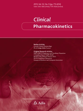
Mathematical functions were derived for each parameter of interest by the mean of weighted linear regression. Linear, polynomial and exponential functions were tested to find the equation that best described the parameter trend. Generally, the regression was performed using sex, age, weight, height, BMI, and BSA as covariates; however, additional covariates were tested if an effect on the parameter of interest was described in the literature (e.g., relationship between blood volume and adipose tissue weight). Covariates were considered significant when their p value was lower than 0.01. To select the best fitted function, we used visual and numeric diagnostics (R2 and Akaike’s information criterion) together with physiological plausibility. The developed equations were implemented in a Matlab® script and were used to generate the virtual population parameter values [21]. The first validation consisted of visually comparing the prediction of 1000 males and females with a BMI ranging from 18.5 to 60 kg/m2 against the independent verification dataset, while the second validation consisted of verifying that the sum of organ weights and blood flows did not exceed body weight and cardiac output. The observed parameters’ variability, expressed as coefficient of variance (CV), was initially estimated as the sum of the covariates’ variability; however, if the CV was not fully captured, an additional random variability with normal distribution was added. The latter was calculated as the observed CV minus the predicted CV, except for the gonads and the pancreas, where the CV was derived from the work of Giwercman et al. [22] and de la Grandmaison et al. [23], respectively. For some parameters, the data were heteroscedastic, however since the increased variability at a higher BMI was overall well-predicted by the variability of the dependent variables, a fixed CV was used rather than a CV depending on BMI (Figs. 1, 2, 3, 4, 5, 6).

Fat-free mass index (a) and fat mass index (b) relative to BMI. The blue, red and black lines represent the predicted mean of virtual male individuals, virtual female individuals and from all virtual subjects, respectively. The area within the two dashed lines represents the 99% normal range. Asterisks represent observed data from the development and circles represent observed data from the independent verification dataset. Male and female data points are represented in light blue and pink, respectively. BMI body mass index

Adipose tissue weight (a) and adipose tissue blood flow (b) relative to BMI. The blue, red and black lines represent the predicted mean of virtual male individuals, virtual female individuals and from all virtual subjects, respectively. The area within the two dashed lines represents the 99% normal range. Asterisks represent observed data from the development and circles represent observed data from the independent verification dataset. Male, female and mixed-sex data points are represented in light blue, pink and black, respectively. Datapoints with multiple individuals are represented as mean ± SD. BMI body mass index, SD standard deviation

Liver weight (a) and liver blood flow (b) relative to BMI. The blue, red and black lines represent the predicted mean of virtual male individuals, virtual female individuals and from all virtual subjects, respectively. The area within the two dashed lines represents the 99% normal range. Asterisks represent observed data from the development and circles represent observed data from the independent verification dataset. Male, female and mixed-sex data points are represented in light blue, pink and black, respectively. Datapoints with multiple individuals are represented as mean ± SD. BMI body mass index, SD standard deviation

Kidney weight (a), kidney blood flow (b), and GFR (c) relative to BMI. The blue, red and black lines represent the predicted mean of virtual male individuals, virtual female individuals and from all virtual subjects, respectively. The area within the two dashed lines represents the 99% normal range. Asterisks represent observed data from the development and circles represent observed data from the independent verification dataset. Male, female and mixed-sex data points are represented in light blue, pink and black, respectively. Datapoints with multiple individuals are represented as mean ± SD. BMI body mass index, GFR glomerular filtration rate, SD standard deviation

Blood weight versus body weight (a), α1-acid glycoprotein (b), and albumin (c) relative to BMI. The blue, red and black lines represent the predicted mean of virtual male individuals, virtual female individuals and from all virtual subjects, respectively. The area within the two dashed lines represents the 99% normal range. Asterisks represent observed data from the development and circles represent observed data from the independent verification dataset. Male, female and mixed-sex data points are represented in light blue, pink and black, respectively. Datapoints with multiple individuals are represented as mean ± SD. BMI body mass index, SD standard deviation

Heart weight (a), heart blood flow (b), and cardiac output (c) relative to BMI. The blue, red and black lines represent the predicted mean of virtual male individuals, virtual female individuals and from all virtual subjects, respectively. The area within the two dashed lines represent the 99% normal range. Asterisks represent observed data from the development and circles represent observed data from the independent verification dataset. Male, female and mixed-sex data points are represented in light blue, pink and black, respectively. Datapoints with multiple individuals are represented as mean ± SD. BMI body mass index, SD standard deviation
3 Results
Overall, 346 articles were screened, of which 209 met the inclusion criteria and were included in the analysis. Studies were excluded from the analysis if the patients’ age and BMI were outside the accepted range, if the most important anthropometric data such as weight or BMI were missing, and if the patients had comorbidities impacting the parameter of interest. Information regarding organ weights, obtained from autopsies or magnetic resonance imaging (MRI), were generally available in the literature, while measurements of regional blood flow and biological parameters, which require more sophisticated methodologies, were limited. Most of the collected parameters were measured in individuals with a BMI up to 60 kg/m2 (as shown in Figs. 1, 2, 3, 4, 5, 6), leaving a knowledge gap for higher BMI values. Table 1 lists the derived equations for each organ and the corresponding population variability expressed as CV.
3.1 Body Composition
Body composition data were obtained from the National Health and Nutrition Examination Survey (NHANES) database [24]. Values collected from 1999 to 2018, using dual energy X-ray absorptiometry (DEXA), were analysed and a total of 3620 data points were selected and randomly divided into development and verification datasets. Following the approach of Kyle et al. [25], the fat mass and fat-free mass were normalized by the square of body height and converted into fat mass index (FMI) and fat-free mass index (FFMI). It was found that, for the same BMI, FFMI was higher in males compared with females, and vice versa for FMI, consistent with previous data showing sex differences in body composition (Fig. 1a, b) [26]. Further details regarding the changes in total body water (TBW) and tissue composition are given in Sect. 3.13.
3.2 Adipose Tissue
3.2.1 Adipose Tissue Weight
The adipose tissue weight was derived from the FMI, which was calculated as the difference between BMI and FFMI. The accuracy of the prediction was verified against data from the NHANES database [24]. The adipose tissue weight was found to increase linearly with BMI, with women having higher adipose tissue weight compared with men with the same BMI. The difference in adipose tissue weight between the two sexes halved from 6 to 3.2 kg when changing from a BMI of 20 kg/m2 to a BMI of 60 kg/m2 (Fig. 2a). Overall, the percentage of adipose tissue doubled from 20% in individuals with a BMI of 20 kg/m2 to 45.5% in individuals with a BMI of 60 kg/m2.
3.2.2 Adipose Tissue Blood Flow
Only a few studies measured the adipose tissue blood flow in obese individuals. The methods used by the authors to quantify the blood flow were 133Xe, 85Kr or 15O-labelled water. Eight of the studies, reporting on data from a total of 173 subjects, were used as the development dataset [27,28,29,30,31,32,33,34], while the remaining six studies, including a total of 139 individuals, composed the verification dataset [35,36,37,38,39,40,41]. The data analysis found that the absolute adipose tissue blood flow (expressed as mL/min/100 g) was lower in obese compared with lean individuals, confirming a lower perfusion of the adipose tissue. However, the total adipose tissue blood flow was found to be 160% higher in obese individuals with a BMI of 60 kg/m2 compared with lean individuals with a BMI of 20 kg/m2, explained by the greater adipose tissue mass (Fig. 2b).
3.3 Liver
3.3.1 Liver Weight
The main organ responsible for drug metabolism is the liver, and accurately predicting its weight is critical for in vitro-in vivo extrapolation. The data from a total of 1937 subjects were collected and used as the development dataset [9, 10, 23, 42,43,44,45,46,47]. The goodness of the equation, derived from the regression, was compared against the verification dataset composed of 164 data points [11, 48, 49]. In males and females with a BMI of 20 kg/m2, the liver weight was 1.7 kg and 1.4 kg, respectively, and increased to a weight of 3.6 kg and 3.0 kg, respectively, in individuals with a BMI of 60 kg/m2 (Fig. 3a). It is known from the literature that there is a strong association between obesity and steatosis, with percentages in the severely obese ranging from 85 to 98% [50, 51]. Furthermore, additional studies showed that the liver fat content can be as much as 40% of the total liver weight [52, 53]. Thus, it is important to emphasize that a higher liver mass does not coincide with higher metabolic active liver parenchyma.
3.3.2 Liver Blood Flow
The literature search yielded 11 studies examining liver blood flow in a total of 336 individuals (Fig. 3b) [33, 54,55,56,57,58,59,60,61,62,63]. The analysis showed that the liver blood flow relative to cardiac output remains constant across BMI values, but when expressed as an absolute value, it increases up to 50% in an obese individual with a BMI of 60 kg/m2 in comparison with an individual with a BMI of 20 kg/m2.
3.3.3 In vitro-in vivo Extrapolation Factors
In vitro-in vivo extrapolation factors are critical physiological parameters that are used in PBPK modelling to scale in vitro data to human. Microsomal proteins per gram liver (MPPGL), hepatocytes per gram liver (HPGL), or homogenate proteins per gram liver (HomPPGL) are essential hepatic scaling factors needed to extrapolate human clearance. Unfortunately, no information on how obesity affects these scaling factors is available in literature. It is known that BMI is strongly correlated with fatty liver infiltration, a medical condition called steatosis that can vary from simple non-alcoholic fatty liver disease (NAFLD) without inflammation to non-alcoholic steatohepatitis (NASH) with active hepatic inflammation [64,65,66,67]. Considering that in obese subjects a substantial part of the liver is only accumulated fat and therefore not all the liver volume is metabolically active, using MPPGL, HPGL and HomPPGL values derived from biopsies of healthy-weight individuals could result in an overprediction of clearance. Sinha et al. proposed scaling in vitro clearance values using only the volume of metabolic active liver, also called lean liver volume (LLV) [68, 69]. We applied the same approach and calculated the LLV by subtracting from the predicted liver volume the fat fraction, which was derived from the correlation plot between liver volume and fat content reported in the study by Hedderich et al. [52].
3.3.4 Hepatic Enzyme and Transporter Activity
Only a few studies describing the cytochrome P450 (CYP) enzyme abundance and activity in obese subjects were available in the literature. Two studies looked at the impact of obesity on CYP3A4 expression and found that both BMI and liver fat content have a negative impact on enzyme abundance, leading to lower levels in both liver and intestine [70, 71]. Krogstad et al. investigated the ex vivo activities of several CYP enzymes using biopsies obtained from patients with a wide range of body weights. The authors found that only hepatic CYP3A activity was significantly negatively correlated to body weight, while CYP2B6, CYP2C8, CYP2D6, CYP2C9, CYP2C19 and CYP1A2 activities were not [72]. The decrease in CYP3A4 abundance was obtained from the slope of the correlation plot between BMI and CYP3A4 expression published by Ulvestad et al. [70].
Clinical studies showed that clearance of CYP2E1 substrates is higher in the obese, however it is unclear which parameter is driving this pharmacokinetic change as activity or expression data are lacking [73, 74].
Some uridine 5′-diphosphate-glucuronosyltranferases (UGT) substrates, such as acetaminophen, oxazepam and lorazepam, have been studied in vivo and the results of the clinical trials show a higher clearance in obese compared with non-obese individuals [75]. These findings are in agreement with ex vivo UGT expression values in mouse [76], however in vitro data showing a positive correlation between body weight and UGT protein abundance in humans are missing.
One study examined the effect of obesity on human hepatic uptake transporters. Organic anion transporting polypeptides (OATP) 1B1, OATP1B3 and OATP2B1, as well as the sodium-dependent uptake transporter, were studied in a cohort of individuals with different body weights and only the abundance of OATP1B1 was found to decrease with body weight, while the others remained unchanged [77].
3.4 Kidney
3.4.1 Kidney Weight
The kidney weight equation was derived using data from 1451 subjects collected from six studies [9, 10, 45, 47, 78, 79], and validated against an additional dataset of 168 subjects (Fig. 4a) [11, 48, 49]. Overall, kidney weight increased in both sexes by 17.5% per every 10 BMI bands, up to a BMI of 35 kg/m2, after which the increase was about 8%.
3.4.2 Kidney Blood Flow
Obesity does alter renal function. While organ weight increases across BMI values, the number of glomeruli does not, leading to greater glomerular size and planar surface area. These structural changes occur together with haemodynamic alterations such as higher plasma blood flow and GFR [80]. Based on the data collected from 18 studies describing the changes in renal blood flow [15, 58, 59, 61, 62, 81,82,83,84,85,86,87,88,89,90,91,92,93], we found that absolute kidney blood flow positively correlates with BMI (Fig. 4b), while blood flow relative to cardiac output remains constant at around 20% in males and 18.5% in females.
3.4.3 Glomerular Filtration Rate
The GFR is an important parameter with a key role for the passive elimination of drugs. GFR can be calculated using creatinine-based equations, such as the Cockcroft–Gault formula or the Modification of Diet in Renal Disease (MDRD) equation, but their predictivity is biased in the obese due to higher urine creatinine excretion [94]. For this reason, only data derived using Tc-DTPA and 125I-iothalamate were considered for both the development [15] and validation datasets [95, 96]. In healthy-weight male and female individuals, GFR was found to be 119 and 107 mL/min, respectively, increasing up to 145 and 130 mL/min, respectively, in obese individuals, and reaching 166 and 145 mL/min, respectively, in the morbidly obese (Fig. 4c).
3.5 Blood
3.5.1 Blood Weight
Obesity is linked to an increase in lean body weight and adipose tissue weight, which translates into higher metabolic demand, resulting in greater blood volume (Fig. 5a) [97]. Even if the absolute blood volume is higher in obese subjects, the ratio between blood volume and body weight does not remain constant but decreases. This is explained by the fact that adipose tissue is not highly perfused and therefore requires less blood than the lean mass. Analysis of the blood volume data compiled from the literature [61, 98,99,100,101,102,103,104,105] resulted in a positive correlation with total body weight, with morbidly obese patients with a BMI of 60 kg/m2 having twice the amount of blood compared with a lean subject with a BMI of 20 kg/m2. Additionally, in agreement with previous observations, we found that the increase in blood weight became less prominent at higher adipose tissue percentages [104].
3.5.2 Haematocrit
Haematocrit was evaluated using a dataset of 764 individuals, with the analysis resulting in sex being the only significant covariate [84, 98,99,100,101,102, 106,107,108]. Males had a mean haematocrit of 0.45, while females had a mean haematocrit of 0.41.
3.5.3 Plasma Protein Concentration
α-Acidic glycoprotein (AAG) levels of 455 individuals with different grades of obesity were collected from 12 studies and were subsequently analysed [109,110,111,112,113,114,115,116,117,118,119,120,121]. AAG concentrations increased from 0.73 to 1.01 g/L in healthy-weight individuals compared with morbidly obese subjects (Fig. 5b).
A negative correlation was found between albumin concentration and BMI, with a constant decline of about 0.41% at each BMI value (Fig. 5c) [109,110,111,112,113,114, 117, 122,123,124,125,126,127,128,129,130].
3.6 Heart
3.6.1 Heart Weight
Higher blood volume and cardiac output in obese subjects are the main causes leading to heart hypertrophy (Fig. 6a) [131, 132]. We investigated the change in heart weight across BMI values by analysing the data of 1203 subjects collected from four published studies [8, 9, 133, 134] and found that age and lean body weight were the two covariates that best described the increase in heart weight. In morbidly obese individuals, the heart reached a weight of 0.55 kg, 85% heavier than in a subject with a BMI of 20 kg/m2.
3.6.2 Heart Blood Flow
Data from 499 subjects and 11 different scientific articles were gathered from the literature [135,136,137,138,139,140,141,142,143,144,145]. Both absolute and relative values of heart blood flow were increased in obese subjects compared with lean-weight subjects. The latter changed from 5.9% in healthy-weight individuals to 7.3% in obese individuals (Fig. 6b).
3.6.3 Cardiac Output
Cardiac output represents the volume of blood pumped by the heart per unit of time. It is calculated as the product of end diastolic volume, ejection fraction, and heart rate. Data from Dini et al. [12] were analysed as the development dataset and subsequently compared against data from another 15 studies [9, 61, 97, 105, 146,147,148,149,150,151,152,153,154,155,156]. Heart rate was found to not change with obesity in accordance with other studies [132]. Furthermore, end diastolic volume increased proportionally to blood volume, while ejection fraction decreased slightly across BMI values. Multiplication of the three parameters leads to an increase in cardiac output of about 10% every 10 BMI bands, starting from 5.1 L/min in healthy-weight subjects to 5.9 L/min in obese individuals, and up to 7.5 L/min in morbidly obese individuals with a BMI of 60 kg/m2 (Fig. 6c).
3.7 Gastrointestinal Tract
3.7.1 Gastrointestinal Tract Weight
Only one study compared stomach weight between lean and obese individuals, with the authors of that study reporting no differences between the two groups [157]. With regard to small and large intestine weight, no information was available in the literature. Studies regarding small bowel length were conducted but controversial conclusions were found. Despite this, the latest studies performed with more subjects found no correlations between intestinal length and body weight [158, 159]. Small bowel length was derived using the equation proposed by Tacchino et al. [159], while large bowel length was obtained using the equation proposed by the ICRP [16]. Intestinal weight was then calculated assuming that the intestine has a cylindrical shape and using intestinal length, diameter and thickness data [160, 161].
3.7.2 Gastrointestinal Blood Flow
Small intestine blood flow was found to not increase with obesity [162, 163], therefore absolute blood flow was kept constant across BMI values. No data regarding obese stomach and colon blood flows are currently available in the literature, therefore the absolute blood flow was assumed to not change across BMI values as for the small intestine.
3.7.3 Gastric pH
Only a few studies investigated the change in gastric pH. Two studies found the obese group to have a slightly lower gastric pH compared with the lean group (median values were 2.3 vs. 2.8, and 1.3 vs. 3.7, respectively) [164, 165], while a third study reported no difference (1.69 vs. 1.65) [166]. However, when comparing their results with gastric pH in young healthy volunteers measured in other studies (median values 1.72 and 1.45), we found no correlation with BMI [167,168,169] and therefore used the same gastric pH in lean subjects as in obese individuals.
3.7.4 Gastrointestinal Transit Time
Gastric and small bowel transit times have been studied over the years using different methods and a variety of test meals, leading to conflicting conclusions. Some articles reported a faster transit time [170, 171], while others reported a similar transit time [172,173,174,175,176,177], and some even reported a delayed transit time [178, 179], in obese compared with lean individuals. However, more recent papers all point to the same conclusions, i.e. both gastric transit time and small bowel transit time are similar between the two groups [172,173,174].
3.7.5 Passive Permeability
Passive permeability was reported to be higher in obese individuals [180], however the method used to investigate the change was based on urine excretion of orally administered mannitol and lactulose without correction for the obesity-dependent increase in GFR. Therefore, it is not clear whether the higher concentration of mannitol and lactulose in urine are related to higher absorption or higher excretion.
3.8 Brain Weight and Blood Flow
Obesity can cause a small reduction in brain volume. One study observed an up to 2.4% reduction in grey matter volume in obese patients [181, 182]. Unfortunately, data gathered from the literature were insufficient to derive a descriptive equation, therefore the equation from Stader et al. [5] was taken and verified against the data of Young et al. [9]. On the other hand, only one study examined brain blood flow in obese individuals and it was found to decrease by 0.34 mL/100 g/min per BMI [183].
3.9 Muscle
3.9.1 Muscle Weight
The total skeletal muscle weight was calculated from the DEXA instrument data obtained from the NHANES database [24], following the approach proposed by Kim et al. [184]. A total of 3620 data points were analysed and compared against 413 MRI data [185]. The increase in muscle weight was about 24.7% for each 10 BMI units, up to a BMI of 40 kg/m2, and 13.8% afterwards.
3.9.2 Muscle Blood Flow
Eleven studies investigated muscle blood flow in healthy and obese individuals, and a total of 361 data points were used for deriving the descriptive function [28, 41, 186,187,188,189,190,191,192,193,194]. The analysis revealed a decrease in blood flow relative to cardiac output, from 15.7 and 12.6% in healthy-weight males and females, respectively, to 13.4 and 10.7% in obese subjects and up to 11.9 and 9.5% in morbidly obese individuals, respectively.
3.10 Skeleton Weight and Blood Flow
The skeleton weight equation was derived from the body bone mineral content data gathered from the NHANES database [24] and verified against dissected skeleton weight data [195]. In accordance with the study by Dolan et al., skeleton weight increased proportionally with body height and body weight but decreased with higher percentages of adipose mass [196]. On average, skeleton weight was 11 and 22% heavier in obese and morbidly obese individuals, respectively. No information regarding the effect of obesity on bone blood flow was available in the literature, therefore we assumed it was identical to the healthy population [5] and constant across BMI values.
3.11 Skin Weight and Blood Flow
Data on skin weight in obese individuals were lacking in the literature, therefore we took the equation suggested by Kerr [197] and compared it against a small dataset of 49 subjects aged between 22 and 94 years (we also included elderly patients since only a few data were available and they were not used for the development of the equation) [198]. Due to the lack of data on skin blood flow, we used the data measured in a wide cohort of Tunisian women; however, since the data were expressed as arbitrary units rather than mL/100 g/min, we applied the same slope to the calculated absolute blood flow, assuming no difference in slope between Caucasian and Berber populations [199, 200].
3.12 Other Organs
Additional organs were studied, with the following information being identified. Spleen weight increased from about 0.19 and 0.15 kg, in lean males and females, respectively, to 0.35 and 0.26 kg, respectively, in the morbidly obese [9,10,11, 23, 49]. Pancreas weight, which was derived using data from two studies, was found to increase about 1.2% at each BMI value [23, 201]. Lungs weight was constant across the BMI—on average, 1.38 kg in males and 1.14 kg in females [9,10,11, 23, 45, 78]. Only one study examined the change of thymus weight across body weight and reported a positive correlation between the two [202]. Data describing the weight change of gonads in obese subjects were missing from the literature and therefore it was assumed to be constant across body weights [16, 22].
Only two studies looked at pancreas blood flow in obese versus lean individuals and found that pancreas perfusion is lower in obese subjects [203, 204]. Calculation of pancreas blood flow is actually a novelty since it is derived from human data and not taken from the ICRP [16], which refers to the paper by Williams and Leggett, where they extrapolated pancreas blood flow from animal data [19].
Unfortunately, blood flow data were not available in the literature for spleen, thymus, and gonads and they were therefore assumed to be constant across BMI values.
Information regarding the weight of the lymphatic system in obese subjects was lacking. However, on the other hand, several studies showed that obesity can have a negative effect on the functionality of the lymphatic system [205]. In obese subjects, there was a reduction of about 30% in the capacity of the lymphatic system in removing macromolecules from adipose tissue [31].
Figure 7a, b provide an overall picture of how body composition, expressed as a percentage of organ weight, and organ haemodynamics, expressed as a percentage of cardiac output, change up to a BMI of 60 kg/m2 in the general population.

Obesity-related changes in organ weights (a) and organ blood flows (b) in the general population. In panel (b), the area within the two dashed line corresponds to the liver blood flow. BMI body mass index
3.13 Tissue Composition
To correctly estimate the partition coefficients of a drug, and thereby the volume of distribution, detailed information on tissue composition is essential. In the literature, information on lipid and protein fractions for each organ across different BMI values were missing; however, we found a few studies analysing the changes in TBW, extracellular body water (EBW), and intracellular body water (IBW) in obese subjects [88, 206,207,208,209,210,211,212,213,214,215,216,217,218,219,220,221,222,223,224]. The absolute TBW was found to increase with BMI (Fig. 8), but when normalized by body weight, obese subjects had a lower ratio compared with healthy-weight subjects. To verify the ability of the model to predict body water distribution, we multiplied the tissue composition factors [225] by the tissue volumes and compared the results against the literature data. By keeping the tissue composition factors constant across BMI values, TBW and IBW resulted in an overprediction, while EBW did not. We therefore adjusted the fractions by lowering the IBW by 0.52% for each BMI and increasing the neutral lipids by 0.52% for each BMI.

Total body water relative to BMI. The blue, red and black lines represent the predicted mean of virtual male individuals, virtual female individuals and from all virtual subjects, respectively. The area within the two dashed lines represents the 99% normal range. Asterisks represent observed data from the development dataset. Male and female sex data points are represented in light blue and pink, respectively. Datapoints with multiple individuals are represented as mean ± SD. BMI body mass index, SD standard deviation
4 Discussion
PBPK modelling is increasingly used to investigate drug pharmacokinetics in special populations; thus, it is critical to develop repositories including anatomical, physiological, and biological parameters to inform PBPK frameworks and subsequently simulate drug disposition for the corresponding population.
A repository describing obese physiology was published by Ghobadi et al. in 2011 [7]; however since then, new data on anatomical, physiological, and biological parameters have been published. Additionally, in the previous work, the authors created two separate populations, one for the obese and one for the morbidly obese, therefore the continuous effect of obesity on parameters was not evaluated. Hence, we aimed to provide an updated repository on the physiological changes induced by different levels of obesity, together with continuous equations and their corresponding physiological variabilities, in order to predict system parameters within a BMI range of 18.5–60 kg/m2.
Our analysis shows that obesity leads to a series of anatomical, physiological, and biological changes, some of which are more relevant than others since they occur in organs responsible for drug elimination (liver and kidney) or absorption (gut), or in tissues critical for drug distribution (adipose and skeletal muscle tissues). The effects of obesity on the liver were found to be higher liver weight and absolute liver blood flow, lower MPPGL and HPGL, and decreased CYP3A4 enzyme abundance. Similarly, obesity resulted in higher kidney weight and greater absolute renal blood flow as well as GFR. These changes lead to higher renal excretion, as previously reported for drugs eliminated primarily by the kidneys [4]. In the long run, these changes may lead to the development of chronic kidney disease in some obese individuals [226]. Another effect of obesity impacting drug disposition is the increase in volume of distribution and half-life [227, 228]. This can be explained by the increase in adipose and skeletal muscle tissue, and lower blood perfusion of the adipose tissue; they act as reservoirs where the drug can initially accumulate and then release slowly over time. Another important parameter that influences drug distribution is tissue composition. We found that IBW was overpredicted by using constant tissue composition factors, meaning that the fraction of IBW decreases at a higher BMI while lipid fraction in the cells tends to increase, as happens for the adipose tissue and the liver [229, 230]. However, studies investigating how each organ composition changes across different BMI values were not available in the literature.
Overall, rich datasets were available for almost all organ weights and for adipose, liver, and muscle blood flow; however, there was a paucity of data for organ weight and organ blood flow above BMI values of 60 and 40 kg/m2, respectively. We therefore decided to stop the validity of the equations at a BMI of 60 kg/m2. Additionally, it may not be useful to go beyond a BMI of 60 kg/m2 since clinical trials in this subpopulation are difficult to find. For some parameters, limited information across the whole BMI range were reported in the literature. In particular, no data were available for MPPGL, HPGL, or HomPPGL, which are key parameters necessary to accurately perform the in vitro-in vivo calculations; even information on the abundance of enzymes and transporters were limited and sometimes contradictory. However, we filled these gaps by making physiologically plausible assumptions (e.g. to overcome the lack of MPPGL, HPGL, or HomPPGL in obese subjects, we kept their values constant and scaled them using only LLV. Overall, the population is robust up to a BMI of 40 kg/m2 and less robust with a BMI between 40 and 60 kg/m2 due to extrapolation of the organ blood flow (Figs. 1, 2, 3, 4, 5, 6).
Nowadays, the obese population represents about 13% of the worldwide population, and even if this represents a large proportion of individuals, clinical information on drug dosing, pharmacokinetics, or drug–drug interactions magnitude in this special population are still missing. This relates to the fact that obese individuals are often underrepresented in clinical trials. The current repository provides an updated description of the physiology of an obese population with a BMI up to 60 kg/m2 by using continuous functions and physiologic variability for each parameter. It can be implemented in current PBPK models, enabling pharmacometricians to simulate difficult clinical scenarios in this special population and thereby filling the existing knowledge gaps around the magnitude of individualized drug therapy, drug disposition, and drug–drug interactions.
5 Conclusions
The developed repository provides up-to-date data on the anatomical, physiological, and biological changes induced by obesity. It highlights areas where knowledge gaps still exist and where further research is needed. Nonetheless, the derived continuous equations and the corresponding population variability in subjects with a BMI up to 60 kg/m2 provide a good description of several key system parameters. Finally, this database is a valuable tool that can be added to existing PBPK models to investigate the pharmacokinetics and support informed decision making regarding optimal dosing regimens in this special population.
References
World Health Organization. Obesity and overweight. Available at: https://www.who.int/news-room/fact-sheets/detail/obesity-and-overweight. Accessed 4 Nov 2021.
Guh DP, Zhang W, Bansback N, Amarsi Z, Birmingham CL, Anis AH. The incidence of co-morbidities related to obesity and overweight: a systematic review and meta-analysis. BMC Public Health. 2009;9:88.
Hruby A, Hu FB. The epidemiology of obesity: a big picture. Pharmacoeconomics. 2015;33(7):673–89.
Brill MJ, Diepstraten J, van Rongen A, van Kralingen S, van den Anker JN, Knibbe CA. Impact of obesity on drug metabolism and elimination in adults and children. Clin Pharmacokinet. 2012;51(5):277–304.
Stader F, Siccardi M, Battegay M, Kinvig H, Penny MA, Marzolini C. Repository describing an aging population to inform physiologically based pharmacokinetic models considering anatomical, physiological, and biological age-dependent changes. Clin Pharmacokinet. 2019;58(4):483–501.
Dallmann A, Ince I, Meyer M, Willmann S, Eissing T, Hempel G. Gestation-specific changes in the anatomy and physiology of healthy pregnant women: an extended repository of model parameters for physiologically based pharmacokinetic modeling in pregnancy. Clin Pharmacokinet. 2017;56(11):1303–30.
Ghobadi C, Johnson TN, Aarabi M, Almond LM, Allabi AC, Rowland-Yeo K, et al. Application of a systems approach to the bottom-up assessment of pharmacokinetics in obese patients: expected variations in clearance. Clin Pharmacokinet. 2011;50(12):809–22.
Vanhaebost J, Faouzi M, Mangin P, Michaud K. New reference tables and user-friendly Internet application for predicted heart weights. Int J Legal Med. 2014;128(4):615–20.
Young JF, Luecke RH, Pearce BA, Lee T, Ahn H, Baek S, et al. Human organ/tissue growth algorithms that include obese individuals and black/white population organ weight similarities from autopsy data. J Toxicol Environ Health A. 2009;72(8):527–40.
Brodsky SV, Gruszecki AC, Fallon K, Pasquale-Styles MA, Shaddy S, Yildiz V, et al. Morphometric data on severely and morbidly obese deceased, established on forensic and non-forensic autopsies. Virchows Arch. 2016;469(4):451–8.
Mandal R, Loeffler AG, Salamat S, Fritsch MK. Organ weight changes associated with body mass index determined from a medical autopsy population. Am J Forensic Med Pathol. 2012;33(4):382–9.
Dini FL, Fabiani I, Miccoli M, Galeotti GG, Pugliese NR, D’Agostino A, et al. Prevalence and determinants of left ventricular diastolic dysfunction in obese subjects and the role of left ventricular global longitudinal strain and mass normalized to height. Echocardiography. 2018;35(8):1124–31.
Chew-Harris JS, Florkowski CM, George PM, Endre ZH. Comparative performances of the new chronic kidney disease epidemiology equations incorporating cystatin C for use in cancer patients. Asia Pac J Clin Oncol. 2015;11(2):142–51.
Kwakernaak AJ, Toering TJ, Navis G. Body mass index and body fat distribution as renal risk factors: a focus on the role of renal haemodynamics. Nephrol Dial Transplant. 2013;28(Suppl 4):iv42–9.
Kwakernaak AJ, Zelle DM, Bakker SJ, Navis G. Central body fat distribution associates with unfavorable renal hemodynamics independent of body mass index. J Am Soc Nephrol. 2013;24(6):987–94.
Valentin J. Basic anatomical and physiological data for use in radiological protection: reference values. ICRP Publication 89. Ann ICRP. 2002;32(3):1–277.
Hozo SP, Djulbegovic B, Hozo I. Estimating the mean and variance from the median, range, and the size of a sample. BMC Med Res Methodol. 2005;5:13.
Wan X, Wang W, Liu J, Tong T. Estimating the sample mean and standard deviation from the sample size, median, range and/or interquartile range. BMC Med Res Methodol. 2014;14:135.
Williams LR, Leggett RW. Reference values for resting blood flow to organs of man. Clin Phys Physiol Meas. 1989;10(3):187–217.
Ashby-Thompson M, Ji Y, Wang J, Yu W, Thornton JC, Wolper C, et al. High-resolution three-dimensional photonic scan-derived equations improve body surface area prediction in diverse populations. Obesity (Silver Spring). 2020;28(4):706–17.
Stader F, Penny MA, Siccardi M, Marzolini C. A comprehensive framework for physiologically based pharmacokinetic modelling in Matlab. CPT Pharmacometr Syst Pharmacol. 2019;8(7):444–59.
Giwercman A, Muller J, Skakkebaek NE. Prevalence of carcinoma in situ and other histopathological abnormalities in testes from 399 men who died suddenly and unexpectedly. J Urol. 1991;145(1):77–80.
de la Grandmaison GL, Clairand I, Durigon M. Organ weight in 684 adult autopsies: new tables for a Caucasoid population. Forensic Sci Int. 2001;119(2):149–54.
Centers for Disease Control and Prevention. National Health and Nutrition Examination Survey. Available at: https://wwwn.cdc.gov/nchs/nhanes/Default.aspx. Accessed 12 Oct 2020.
Kyle UG, Schutz Y, Dupertuis YM, Pichard C. Body composition interpretation. Contributions of the fat-free mass index and the body fat mass index. Nutrition. 2003;19(7–8):597–604.
Lemieux S, Prud’homme D, Bouchard C, Tremblay A, Despres JP. Sex differences in the relation of visceral adipose tissue accumulation to total body fatness. Am J Clin Nutr. 1993;58(4):463–7.
Blaak EE, van Baak MA, Kemerink GJ, Pakbiers MT, Heidendal GA, Saris WH. Beta-adrenergic stimulation and abdominal subcutaneous fat blood flow in lean, obese, and reduced-obese subjects. Metabolism. 1995;44(2):183–7.
Dadson P, Ferrannini E, Landini L, Hannukainen JC, Kalliokoski KK, Vaittinen M, et al. Fatty acid uptake and blood flow in adipose tissue compartments of morbidly obese subjects with or without type 2 diabetes: effects of bariatric surgery. Am J Physiol Endocrinol Metab. 2017;313(2):E175–82.
Asmar M, Simonsen L, Arngrim N, Holst JJ, Dela F, Bulow J. Glucose-dependent insulinotropic polypeptide has impaired effect on abdominal, subcutaneous adipose tissue metabolism in obese subjects. Int J Obes (Lond). 2014;38(2):259–65.
Andersson J, Karpe F, Sjostrom LG, Riklund K, Soderberg S, Olsson T. Association of adipose tissue blood flow with fat depot sizes and adipokines in women. Int J Obes (Lond). 2012;36(6):783–9.
Arngrim N, Simonsen L, Holst JJ, Bulow J. Reduced adipose tissue lymphatic drainage of macromolecules in obese subjects: a possible link between obesity and local tissue inflammation? Int J Obes (Lond). 2013;37(5):748–50.
Jansson PA, Larsson A, Smith U, Lonnroth P. Glycerol production in subcutaneous adipose tissue in lean and obese humans. J Clin Invest. 1992;89(5):1610–7.
Enevoldsen LH, Simonsen L, Macdonald IA, Bulow J. The combined effects of exercise and food intake on adipose tissue and splanchnic metabolism. J Physiol. 2004;561(Pt 3):871–82.
Lesser GT, Deutsch S. Measurement of adipose tissue blood flow and perfusion in man by uptake of 85Kr. J Appl Physiol. 1967;23(5):621–30.
Blaak EE, van Baak MA, Kemerink GJ, Pakbiers MT, Heidendal GA, Saris WH. Total forearm blood flow as an indicator of skeletal muscle blood flow: effect of subcutaneous adipose tissue blood flow. Clin Sci (Lond). 1994;87(5):559–66.
Summers LK, Samra JS, Humphreys SM, Morris RJ, Frayn KN. Subcutaneous abdominal adipose tissue blood flow: variation within and between subjects and relationship to obesity. Clin Sci (Lond). 1996;91(6):679–83.
Viljanen AP, Lautamaki R, Jarvisalo M, Parkkola R, Huupponen R, Lehtimaki T, et al. Effects of weight loss on visceral and abdominal subcutaneous adipose tissue blood-flow and insulin-mediated glucose uptake in healthy obese subjects. Ann Med. 2009;41(2):152–60.
Blaak EE, Van Baak MA, Kemerink GJ, Pakbiers MT, Heidendal GA, Saris WH. Beta-adrenergic stimulation of energy expenditure and forearm skeletal muscle metabolism in lean and obese men. Am J Physiol. 1994;267(2 Pt 1):E306–15.
Jansson PA, Larsson A, Lonnroth PN. Relationship between blood pressure, metabolic variables and blood flow in obese subjects with or without non-insulin-dependent diabetes mellitus. Eur J Clin Invest. 1998;28(10):813–8.
Simonsen L, Henriksen O, Enevoldsen LH, Bulow J. The effect of exercise on regional adipose tissue and splanchnic lipid metabolism in overweight type 2 diabetic subjects. Diabetologia. 2004;47(4):652–9.
Pitkanen OP, Laine H, Kemppainen J, Eronen E, Alanen A, Raitakari M, et al. Sodium nitroprusside increases human skeletal muscle blood flow, but does not change flow distribution or glucose uptake. J Physiol. 1999;15(521 Pt 3):729–37.
Chouker A, Martignoni A, Dugas M, Eisenmenger W, Schauer R, Kaufmann I, et al. Estimation of liver size for liver transplantation: the impact of age and gender. Liver Transpl. 2004;10(5):678–85.
Molina DK, DiMaio VJ. Normal organ weights in men: part II—the brain, lungs, liver, spleen, and kidneys. Am J Forensic Med Pathol. 2012;33(4):368–72.
Thompson CM, Johns DO, Sonawane B, Barton HA, Hattis D, Tardif R, et al. Database for physiologically based pharmacokinetic (PBPK) modeling: physiological data for healthy and health-impaired elderly. J Toxicol Environ Health B Crit Rev. 2009;12(1):1–24.
Calloway NO, Foley CF, Lagerbloom P. Uncertainties in geriatric data. II. Organ size. J Am Geriatr Soc. 1965;13:20–8.
Basic anatomical and physiological data for use in radiological protection: reference values. A report of age- and gender-related differences in the anatomical and physiological characteristics of reference individuals. ICRP Publication 89. Ann ICRP. 2002;32(3–4):5-265.
Gallagher D, Belmonte D, Deurenberg P, Wang Z, Krasnow N, Pi-Sunyer FX, et al. Organ-tissue mass measurement allows modeling of REE and metabolically active tissue mass. Am J Physiol. 1998;275(2):E249–58.
Bosy-Westphal A, Kossel E, Goele K, Later W, Hitze B, Settler U, et al. Contribution of individual organ mass loss to weight loss-associated decline in resting energy expenditure. Am J Clin Nutr. 2009;90(4):993–1001.
Bosy-Westphal A, Reinecke U, Schlorke T, Illner K, Kutzner D, Heller M, et al. Effect of organ and tissue masses on resting energy expenditure in underweight, normal weight and obese adults. Int J Obes Relat Metab Disord. 2004;28(1):72–9.
Machado M, Marques-Vidal P, Cortez-Pinto H. Hepatic histology in obese patients undergoing bariatric surgery. J Hepatol. 2006;45(4):600–6.
Marceau P, Biron S, Hould FS, Marceau S, Simard S, Thung SN, et al. Liver pathology and the metabolic syndrome X in severe obesity. J Clin Endocrinol Metab. 1999;84(5):1513–7.
Hedderich DM, Hasenberg T, Haneder S, Schoenberg SO, Kucukoglu O, Canbay A, et al. Effects of bariatric surgery on non-alcoholic fatty liver disease: magnetic resonance imaging is an effective, non-invasive method to evaluate changes in the liver fat fraction. Obes Surg. 2017;27(7):1755–62.
Noureddin M, Lam J, Peterson MR, Middleton M, Hamilton G, Le TA, et al. Utility of magnetic resonance imaging versus histology for quantifying changes in liver fat in nonalcoholic fatty liver disease trials. Hepatology. 2013;58(6):1930–40.
Felig P, Wahren J, Hendler R, Brundin T. Splanchnic glucose and amino acid metabolism in obesity. J Clin Invest. 1974;53(2):582–90.
Nielsen S, Guo Z, Johnson CM, Hensrud DD, Jensen MD. Splanchnic lipolysis in human obesity. J Clin Invest. 2004;113(11):1582–8.
Peiris AN, Mueller RA, Smith GA, Struve MF, Kissebah AH. Splanchnic insulin metabolism in obesity. Influence of body fat distribution. J Clin Invest. 1986;78(6):1648–57.
Ludvik B, Nolan JJ, Roberts A, Baloga J, Joyce M, Bell JM, et al. A noninvasive method to measure splanchnic glucose uptake after oral glucose administration. J Clin Invest. 1995;95(5):2232–8.
Minson CT, Wladkowski SL, Cardell AF, Pawelczyk JA, Kenney WL. Age alters the cardiovascular response to direct passive heating. J Appl Physiol (1985). 1998;84(4):1323–32.
Ho CW, Beard JL, Farrell PA, Minson CT, Kenney WL. Age, fitness, and regional blood flow during exercise in the heat. J Appl Physiol (1985). 1997;82(4):1126–35.
Wynne HA, Cope LH, Mutch E, Rawlins MD, Woodhouse KW, James OF. The effect of age upon liver volume and apparent liver blood flow in healthy man. Hepatology. 1989;9(2):297–301.
Messerli FH, Sundgaard-Riise K, Reisin E, Dreslinski G, Dunn FG, Frohlich E. Disparate cardiovascular effects of obesity and arterial hypertension. Am J Med. 1983;74(5):808–12.
Messerli FH, Ventura HO, Reisin E, Dreslinski GR, Dunn FG, MacPhee AA, et al. Borderline hypertension and obesity: two prehypertensive states with elevated cardiac output. Circulation. 1982;66(1):55–60.
Nelson RH, Basu R, Johnson CM, Rizza RA, Miles JM. Splanchnic spillover of extracellular lipase-generated fatty acids in overweight and obese humans. Diabetes. 2007;56(12):2878–84.
Moretto M, Kupski C, Mottin CC, Repetto G, Garcia Toneto M, Rizzolli J, et al. Hepatic steatosis in patients undergoing bariatric surgery and its relationship to body mass index and co-morbidities. Obes Surg. 2003;13(4):622–4.
Harnois F, Msika S, Sabate JM, Mechler C, Jouet P, Barge J, et al. Prevalence and predictive factors of non-alcoholic steatohepatitis (NASH) in morbidly obese patients undergoing bariatric surgery. Obes Surg. 2006;16(2):183–8.
Pienkowska J, Brzeska B, Kaszubowski M, Kozak O, Jankowska A, Szurowska E. MRI assessment of ectopic fat accumulation in pancreas, liver and skeletal muscle in patients with obesity, overweight and normal BMI in correlation with the presence of central obesity and metabolic syndrome. Diabetes Metab Syndr Obes. 2019;12:623–36.
Pasanta D, Tungjai M, Chancharunee S, Sajomsang W, Kothan S. Body mass index and its effects on liver fat content in overweight and obese young adults by proton magnetic resonance spectroscopy technique. World J Hepatol. 2018;10(12):924–33.
Sinha J, Duffull SB, Green B, Al-Sallami HS. Evaluating the relationship between lean liver volume and fat-free mass. Clin Pharmacokinet. 2020;59(4):475–83.
Sinha J, Duffull SB, Green B, Al-Sallami HS. Evaluating lean liver volume as a potential scaler for in vitro-in vivo extrapolation of drug clearance in obesity using the model drug antipyrine. Curr Drug Metab. 2020;21(10):746–50.
Ulvestad M, Skottheim IB, Jakobsen GS, Bremer S, Molden E, Asberg A, et al. Impact of OATP1B1, MDR1, and CYP3A4 expression in liver and intestine on interpatient pharmacokinetic variability of atorvastatin in obese subjects. Clin Pharmacol Ther. 2013;93(3):275–82.
Jamwal R, de la Monte SM, Ogasawara K, Adusumalli S, Barlock BB, Akhlaghi F. Nonalcoholic fatty liver disease and diabetes are associated with decreased CYP3A4 protein expression and activity in human liver. Mol Pharm. 2018;15(7):2621–32.
Krogstad V, Peric A, Robertsen I, Kringen MK, Vistnes M, Hjelmesaeth J, et al. Correlation of body weight and composition with hepatic activities of cytochrome P450 enzymes. J Pharm Sci. 2021;110(1):432–7.
Emery MG, Fisher JM, Chien JY, Kharasch ED, Dellinger EP, Kowdley KV, et al. CYP2E1 activity before and after weight loss in morbidly obese subjects with nonalcoholic fatty liver disease. Hepatology. 2003;38(2):428–35.
O’Shea D, Davis SN, Kim RB, Wilkinson GR. Effect of fasting and obesity in humans on the 6-hydroxylation of chlorzoxazone: a putative probe of CYP2E1 activity. Clin Pharmacol Ther. 1994;56(4):359–67.
Abernethy DR, Greenblatt DJ, Divoll M, Shader RI. Enhanced glucuronide conjugation of drugs in obesity: studies of lorazepam, oxazepam, and acetaminophen. J Lab Clin Med. 1983;101(6):873–80.
Xu J, Kulkarni SR, Li L, Slitt AL. UDP-glucuronosyltransferase expression in mouse liver is increased in obesity- and fasting-induced steatosis. Drug Metab Dispos. 2012;40(2):259–66.
Wegler C, Prieto Garcia L, Klinting S, Robertsen I, Wisniewski JR, Hjelmesaeth J, et al. Proteomics-informed prediction of rosuvastatin plasma profiles in patients with a wide range of body weight. Clin Pharmacol Ther. 2021;109(3):762–71.
Molina DK, DiMaio VJ. Normal organ weights in men: part II-the brain, lungs, liver, spleen, and kidneys. Am J Forensic Med Pathol. 2012;33(4):368–72.
Nyengaard JR, Bendtsen TF. Glomerular number and size in relation to age, kidney weight, and body surface in normal man. Anat Rec. 1992;232(2):194–201.
Eknoyan G. Obesity, diabetes, and chronic kidney disease. Curr Diab Rep. 2007;7(6):449–53.
Miller JH, Mc DR, Shock NW. The renal extraction of p-aminohippurate in the aged individual. J Gerontol. 1951;6(3):213–6.
Bauer JH, Brooks CS, Burch RN. Renal function and hemodynamic studies in low- and normal-renin essential hypertension. Arch Intern Med. 1982;142(7):1317–23.
Fliser D, Zeier M, Nowack R, Ritz E. Renal functional reserve in healthy elderly subjects. J Am Soc Nephrol. 1993;3(7):1371–7.
Goldring W, Chasis H, Ranges HA, Smith HW. Relations of effective renal blood flow and glomerular filtration to tubular excretory mass in normal man. J Clin Invest. 1940;19(5):739–50.
Davies DF, Shock NW. Age changes in glomerular filtration rate, effective renal plasma flow, and tubular excretory capacity in adult males. J Clin Invest. 1950;29(5):496–507.
Fuiano G, Sund S, Mazza G, Rosa M, Caglioti A, Gallo G, et al. Renal hemodynamic response to maximal vasodilating stimulus in healthy older subjects. Kidney Int. 2001;59(3):1052–8.
Mc DR, Solomon DH, Shock NW. Aging as a factor in the renal hemodynamic changes induced by a standardized pyrogen. J Clin Invest. 1951;30(5):457–62.
Raison J, Achimastos A, Asmar R, Simon A, Safar M. Extracellular and interstitial fluid volume in obesity with and without associated systemic hypertension. Am J Cardiol. 1986;57(4):223–6.
Frohlich ED, Messerli FH, Reisin E, Dunn FG. The problem of obesity and hypertension. Hypertension. 1983;5(5 Pt 2):III71–8.
Chagnac A, Weinstein T, Korzets A, Ramadan E, Hirsch J, Gafter U. Glomerular hemodynamics in severe obesity. Am J Physiol Renal Physiol. 2000;278(5):F817–22.
Chagnac A, Weinstein T, Herman M, Hirsh J, Gafter U, Ori Y. The effects of weight loss on renal function in patients with severe obesity. J Am Soc Nephrol. 2003;14(6):1480–6.
Ahmed SB, Fisher ND, Stevanovic R, Hollenberg NK. Body mass index and angiotensin-dependent control of the renal circulation in healthy humans. Hypertension. 2005;46(6):1316–20.
Schmieder RE, Beil AH, Weihprecht H, Messerli FH. How should renal hemodynamic data be indexed in obesity? J Am Soc Nephrol. 1995;5(9):1709–13.
Chang AR, Zafar W, Grams ME. Kidney function in obesity-challenges in indexing and estimation. Adv Chronic Kidney Dis. 2018;25(1):31–40.
Chew-Harris JS, Chin PK, Florkowski CM, George P, Endre Z. Removal of body surface area normalisation improves raw-measured glomerular filtration rate estimation by the Chronic Kidney Disease Epidemiology Collaboration equation and drug dosing in the obese. Intern Med J. 2015;45(7):766–73.
Chew-Harris JS, Florkowski CM, Elmslie JL, Livesey J, Endre ZH, George PM. Lean mass modulates glomerular filtration rate in males of normal and extreme body composition. Intern Med J. 2014;44(8):749–56.
Collis T, Devereux RB, Roman MJ, de Simone G, Yeh J, Howard BV, et al. Relations of stroke volume and cardiac output to body composition: the strong heart study. Circulation. 2001;103(6):820–5.
Brown E, Hopper J Jr, Hodges JL Jr, Bradley B, Wennesland R, Yamauchi H. Red cell, plasma, and blood volume in the healthy women measured by radiochromium cell-labeling and hematocrit. J Clin Invest. 1962;41:2182–90.
Wennesland R, Brown E, Hopper J Jr, Hodges JL Jr, Guttentag OE, Scott KG, et al. Red cell, plasma and blood volume in healthy men measured by radiochromium (Cr51) cell tagging and hematocrit: influence of age, somatotype and habits of physical activity on the variance after regression of volumes to height and weight combined. J Clin Invest. 1959;38(7):1065–77.
Huff RL, Feller DD. Relation of circulating red cell volume to body density and obesity. J Clin Invest. 1956;35(1):1–10.
Gibson JG, Evans WA. Clinical studies of the blood volume. II. The relation of plasma and total blood volume to venous pressure, blood velocity rate, physical measurements, age and sex in ninety normal humans. J Clin Invest. 1937;16(3):317–28.
Retzlaff JA, Tauxe WN, Kiely JM, Stroebel CF. Erythrocyte volume, plasma volume, and lean body mass in adult men and women. Blood. 1969;33(5):649–61.
Feldschuh J, Enson Y. Prediction of the normal blood volume. Relation of blood volume to body habitus. Circulation. 1977;56(4 Pt 1):605–12.
Cepeda-Lopez AC, Zimmermann MB, Wussler S, Melse-Boonstra A, Naef N, Mueller SM, et al. Greater blood volume and Hb mass in obese women quantified by the carbon monoxide-rebreathing method affects interpretation of iron biomarkers and iron requirements. Int J Obes (Lond). 2019;43(5):999–1008.
Messerli FH, Christie B, DeCarvalho JG, Aristimuno GG, Suarez DH, Dreslinski GR, et al. Obesity and essential hypertension. Hemodynamics, intravascular volume, sodium excretion, and plasma renin activity. Arch Intern Med. 1981;141(1):81–5.
Smith WW, Wikler NS, Fox AC. Hemodynamic studies of patients with myocardial infarction. Circulation. 1954;9(3):352–62.
Tietz NW, Shuey DF, Wekstein DR. Laboratory values in fit aging individuals–sexagenarians through centenarians. Clin Chem. 1992;38(6):1167–85.
Ernst E, Matrai A. Hematologic data on healthy very old people. JAMA. 1987;258(6):781–2.
Benedek IH, Blouin RA, McNamara PJ. Serum protein binding and the role of increased alpha 1-acid glycoprotein in moderately obese male subjects. Br J Clin Pharmacol. 1984;18(6):941–6.
Benedek IH, Fiske WD 3rd, Griffen WO, Bell RM, Blouin RA, McNamara PJ. Serum alpha 1-acid glycoprotein and the binding of drugs in obesity. Br J Clin Pharmacol. 1983;16(6):751–4.
Cameron M, Donati F, Varin F. In vitro plasma protein binding of neuromuscular blocking agents in different subpopulations of patients. Anesth Analg. 1995;81(5):1019–25.
Cheymol G. Drug pharmacokinetics in the obese. Fundam Clin Pharmacol. 1988;2(3):239–56.
Cheymol G, Poirier JM, Barre J, Pradalier A, Dry J. Comparative pharmacokinetics of intravenous propranolol in obese and normal volunteers. J Clin Pharmacol. 1987;27(11):874–9.
Poirier JM, Le Jeunne C, Cheymol G, Cohen A, Barre J, Hugues FC. Comparison of propranolol and sotalol pharmacokinetics in obese subjects. J Pharm Pharmacol. 1990;42(5):344–8.
Akbay E, Yetkin I, Ersoy R, Kulaksizoglu S, Toruner F, Arslan M. The relationship between levels of alpha1-acid glycoprotein and metabolic parameters of diabetes mellitus. Diabetes Nutr Metab. 2004;17(6):331–5.
Ramirez Alvarado MM, Sanchez Roitz C, Perez Diaz A, Millan BE. Effect of a high saturated fatty acids load on serum concentrations of C-reactive protein, alpha1-antitrypsin, fibrinogen and alpha1-acid glycoprotein in obese women [in Spanish]. Nutr Hosp. 2010;25(1):72–9.
Veering BT, Burm AG, Souverijn JH, Serree JM, Spierdijk J. The effect of age on serum concentrations of albumin and alpha 1-acid glycoprotein. Br J Clin Pharmacol. 1990;29(2):201–6.
Routledge PA, Stargel WW, Kitchell BB, Barchowsky A, Shand DG. Sex-related differences in the plasma protein binding of lignocaine and diazepam. Br J Clin Pharmacol. 1981;11(3):245–50.
Paxton JW, Briant RH. Alpha 1-acid glycoprotein concentrations and propranolol binding in elderly patients with acute illness. Br J Clin Pharmacol. 1984;18(5):806–10.
Denko CW, Gabriel P. Age and sex related levels of albumin, ceruloplasmin, alpha 1 antitrypsin, alpha 1 acid glycoprotein, and transferrin. Ann Clin Lab Sci. 1981;11(1):63–8.
Blain PG, Mucklow JC, Rawlins MD, Roberts DF, Routledge PA, Shand DG. Determinants of plasma alpha 1-acid glycoprotein (AAG) concentrations in health. Br J Clin Pharmacol. 1985;20(5):500–2.
Angus JM. A study of clinical outcomes using serum albumin and percentage of weight loss following nutritional intervention in post-operative bariatric patients. East Tennessee State University; 2007. Available at: https://dc.etsu.edu/etd/2144/.
Gersovitz M, Munro HN, Udall J, Young VR. Albumin synthesis in young and elderly subjects using a new stable isotope methodology: response to level of protein intake. Metabolism. 1980;29(11):1075–86.
Gardner MD, Scott R. Age- and sex-related reference ranges for eight plasma constituents derived from randomly selected adults in a Scottish new town. J Clin Pathol. 1980;33(4):380–5.
Pickart L. Increased ratio of plasma free fatty acids to albumin during normal aging and in patients with coronary heart disease. Atherosclerosis. 1983;46(1):21–8.
Reed AH, Cannon DC, Winkelman JW, Bhasin YP, Henry RJ, Pileggi VJ. Estimation of normal ranges from a controlled sample survey. I. Sex- and age-related influence on the SMA 12–60 screening group of tests. Clin Chem. 1972;18(1):57–66.
Fu A, Nair KS. Age effect on fibrinogen and albumin synthesis in humans. Am J Physiol. 1998;275(6):E1023–30.
Wallace S, Whiting B. Factors affecting drug binding in plasma of elderly patients. Br J Clin Pharmacol. 1976;3(2):327–30.
Garry PJ, Hunt WC, VanderJagt DJ, Rhyne RL. Clinical chemistry reference intervals for healthy elderly subjects. Am J Clin Nutr. 1989;50(5 Suppl):1219–30 (discussion 31-5).
Campion EW, deLabry LO, Glynn RJ. The effect of age on serum albumin in healthy males: report from the Normative Aging Study. J Gerontol. 1988;43(1):M18-20.
Lavie CJ, Alpert MA, Arena R, Mehra MR, Milani RV, Ventura HO. Impact of obesity and the obesity paradox on prevalence and prognosis in heart failure. JACC Heart Fail. 2013;1(2):93–102.
Alpert MA, Omran J, Bostick BP. Effects of obesity on cardiovascular hemodynamics, cardiac morphology, and ventricular function. Curr Obes Rep. 2016;5(4):424–34.
Gaitskell K, Perera R, Soilleux EJ. Derivation of new reference tables for human heart weights in light of increasing body mass index. J Clin Pathol. 2011;64(4):358–62.
Skurdal AC, Nordrum IS. A retrospective study of postmortem heart weight in an adult Norwegian population. Cardiovasc Pathol. 2016;25(6):461–7.
Peterson LR, Herrero P, Schechtman KB, Racette SB, Waggoner AD, Kisrieva-Ware Z, et al. Effect of obesity and insulin resistance on myocardial substrate metabolism and efficiency in young women. Circulation. 2004;109(18):2191–6.
Peterson LR, Soto PF, Herrero P, Mohammed BS, Avidan MS, Schechtman KB, et al. Impact of gender on the myocardial metabolic response to obesity. JACC Cardiovasc Imaging. 2008;1(4):424–33.
Sundell J, Laine H, Luotolahti M, Kalliokoski K, Raitakari O, Nuutila P, et al. Obesity affects myocardial vasoreactivity and coronary flow response to insulin. Obes Res. 2002;10(7):617–24.
Sundell J, Raitakari OT, Viikari J, Kantola I, Nuutila P, Knuuti J. Both BMI and waist circumference are associated with coronary vasoreactivity in overweight and obese men. Obes Facts. 2012;5(5):693–9.
Schindler TH, Cardenas J, Prior JO, Facta AD, Kreissl MC, Zhang XL, et al. Relationship between increasing body weight, insulin resistance, inflammation, adipocytokine leptin, and coronary circulatory function. J Am Coll Cardiol. 2006;47(6):1188–95.
Quercioli A, Pataky Z, Montecucco F, Carballo S, Thomas A, Staub C, et al. Coronary vasomotor control in obesity and morbid obesity: contrasting flow responses with endocannabinoids, leptin, and inflammation. JACC Cardiovasc Imaging. 2012;5(8):805–15.
Quercioli A, Pataky Z, Vincenti G, Makoundou V, Di Marzo V, Montecucco F, et al. Elevated endocannabinoid plasma levels are associated with coronary circulatory dysfunction in obesity. Eur Heart J. 2011;32(11):1369–78.
Bergmann SR, Herrero P, Markham J, Weinheimer CJ, Walsh MN. Noninvasive quantitation of myocardial blood flow in human subjects with oxygen-15-labeled water and positron emission tomography. J Am Coll Cardiol. 1989;14(3):639–52.
Chan SY, Brunken RC, Czernin J, Porenta G, Kuhle W, Krivokapich J, et al. Comparison of maximal myocardial blood flow during adenosine infusion with that of intravenous dipyridamole in normal men. J Am Coll Cardiol. 1992;20(4):979–85.
Senneff MJ, Geltman EM, Bergmann SR. Noninvasive delineation of the effects of moderate aging on myocardial perfusion. J Nucl Med. 1991;32(11):2037–42.
Baliga RR, Rosen SD, Camici PG, Kooner JS. Regional myocardial blood flow redistribution as a cause of postprandial angina pectoris. Circulation. 1998;97(12):1144–9.
Salvadori A, Fanari P, Fontana M, Buontempi L, Saezza A, Baudo S, et al. Oxygen uptake and cardiac performance in obese and normal subjects during exercise. Respiration. 1999;66(1):25–33.
Taylor HL, Brozek J, Keys A. Basal cardiac function and body composition with special reference to obesity. J Clin Invest. 1952;31(11):976–83.
Carroll S, Marshall P, Borkoles E, Ingle L, Barker D, Tan LB. Efficacy of lifestyle intervention on peak exercise cardiac power output and reserve in premenopausal obese females: a randomised pilot study. Int J Cardiol. 2007;119(2):147–55.
de Divitiis O, Fazio S, Petitto M, Maddalena G, Contaldo F, Mancini M. Obesity and cardiac function. Circulation. 1981;64(3):477–82.
Danias PG, Tritos NA, Stuber M, Kissinger KV, Salton CJ, Manning WJ. Cardiac structure and function in the obese: a cardiovascular magnetic resonance imaging study. J Cardiovasc Magn Reson. 2003;5(3):431–8.
Kardassis D, Bech-Hanssen O, Schönander M, Sjöström L, Petzold M, Karason K. Impact of body composition, fat distribution and sustained weight loss on cardiac function in obesity. Int J Cardiol. 2012;159(2):128–33.
Messerli FH, Sundgaard-Riise K, Reisin ED, Dreslinski GR, Ventura HO, Oigman W, et al. Dimorphic cardiac adaptation to obesity and arterial hypertension. Ann Intern Med. 1983;99(6):757–61.
Rozenbaum Z, Topilsky Y, Khoury S, Pereg D, Laufer-Perl M. Association of body mass index and diastolic function in metabolically healthy obese with preserved ejection fraction. Int J Cardiol. 2019;277:147–52.
Tejedor A, Rivas E, Ríos J, Arismendi E, Martinez-Palli G, Delgado S, et al. Accuracy of Vigileo/Flotrac monitoring system in morbidly obese patients. J Crit Care. 2015;30(3):562–6.
Cheymol G, Poirier JM, Carrupt PA, Testa B, Weissenburger J, Levron JC, et al. Pharmacokinetics of beta-adrenoceptor blockers in obese and normal volunteers. Br J Clin Pharmacol. 1997;43(6):563–70.
Karason K, Wallentin I, Larsson B, Sjöström L. Effects of obesity and weight loss on cardiac function and valvular performance. Obes Res. 1998;6(6):422–9.
Csendes A, Burgos AM. Size, volume and weight of the stomach in patients with morbid obesity compared to controls. Obes Surg. 2005;15(8):1133–6.
Teitelbaum EN, Vaziri K, Zettervall S, Amdur RL, Orkin BA. Intraoperative small bowel length measurements and analysis of demographic predictors of increased length. Clin Anat. 2013;26(7):827–32.
Tacchino RM. Bowel length: measurement, predictors, and impact on bariatric and metabolic surgery. Surg Obes Relat Dis. 2015;11(2):328–34.
Cronin CG, Delappe E, Lohan DG, Roche C, Murphy JM. Normal small bowel wall characteristics on MR enterography. Eur J Radiol. 2010;75(2):207–11.
Wiesner W, Mortele KJ, Ji H, Ros PR. Normal colonic wall thickness at CT and its relation to colonic distension. J Comput Assist Tomogr. 2002;26(1):102–6.
Honka H, Koffert J, Kauhanen S, Teuho J, Hurme S, Mari A, et al. Bariatric surgery enhances splanchnic vascular responses in patients with type 2 diabetes. Diabetes. 2017;66(4):880–5.
Koffert J, Stahle M, Karlsson H, Iozzo P, Salminen P, Roivainen A, et al. Morbid obesity and type 2 diabetes alter intestinal fatty acid uptake and blood flow. Diabetes Obes Metab. 2018;20(6):1384–90.
Juvin P, Fevre G, Merouche M, Vallot T, Desmonts JM. Gastric residue is not more copious in obese patients. Anesth Analg. 2001;93(6):1621–2.
Vaughan RW, Bauer S, Wise L. Volume and pH of gastric juice in obese patients. Anesthesiology. 1975;43(6):686–9.
Harter RL, Kelly WB, Kramer MG, Perez CE, Dzwonczyk RR. A comparison of the volume and pH of gastric contents of obese and lean surgical patients. Anesth Analg. 1998;86(1):147–52.
Dressman JB, Berardi RR, Dermentzoglou LC, Russell TL, Schmaltz SP, Barnett JL, et al. Upper gastrointestinal (GI) pH in young, healthy men and women. Pharm Res. 1990;7(7):756–61.
Fallingborg J, Christensen LA, Ingeman-Nielsen M, Jacobsen BA, Abildgaard K, Rasmussen HH. pH-profile and regional transit times of the normal gut measured by a radiotelemetry device. Aliment Pharmacol Ther. 1989;3(6):605–13.
Maltby JR, Pytka S, Watson NC, Cowan RA, Fick GH. Drinking 300 mL of clear fluid two hours before surgery has no effect on gastric fluid volume and pH in fasting and non-fasting obese patients. Can J Anaesth. 2004;51(2):111–5.
Tosetti C, Corinaldesi R, Stanghellini V, Pasquali R, Corbelli C, Zoccoli G, et al. Gastric emptying of solids in morbid obesity. Int J Obes Relat Metab Disord. 1996;20(3):200–5.
Wright RA, Krinsky S, Fleeman C, Trujillo J, Teague E. Gastric emptying and obesity. Gastroenterology. 1983;84(4):747–51.
Buchholz V, Berkenstadt H, Goitein D, Dickman R, Bernstine H, Rubin M. Gastric emptying is not prolonged in obese patients. Surg Obes Relat Dis. 2013;9(5):714–7.
Verdich C, Madsen JL, Toubro S, Buemann B, Holst JJ, Astrup A. Effect of obesity and major weight reduction on gastric emptying. Int J Obes Relat Metab Disord. 2000;24(7):899–905.
Al Hillan A, Curras-Martin D, Carson M, Gor S, Ezeume A, Gupta V, et al. Capsule endoscopy transit time to duodenum: relation to patient demographics. Cureus. 2020;12(2): e6894.
Glasbrenner B, Pieramico O, Brecht-Krauss D, Baur M, Malfertheiner P. Gastric emptying of solids and liquids in obesity. Clin Investig. 1993;71(7):542–6.
Zahorska-Markiewicz B, Jonderko K, Lelek A, Skrzypek D. Gastric emptying in obesity. Hum Nutr Clin Nutr. 1986;40(4):309–13.
Wisen O, Johansson C. Gastrointestinal function in obesity: motility, secretion, and absorption following a liquid test meal. Metabolism. 1992;41(4):390–5.
Horowitz M, Collins PJ, Cook DJ, Harding PE, Shearman DJ. Abnormalities of gastric emptying in obese patients. Int J Obes. 1983;7(5):415–21.
Maddox A, Horowitz M, Wishart J, Collins P. Gastric and oesophageal emptying in obesity. Scand J Gastroenterol. 1989;24(5):593–8.
Ott B, Skurk T, Hastreiter L, Lagkouvardos I, Fischer S, Buttner J, et al. Effect of caloric restriction on gut permeability, inflammation markers, and fecal microbiota in obese women. Sci Rep. 2017;7(1):11955.
Hamer M, Batty GD. Association of body mass index and waist-to-hip ratio with brain structure: UK Biobank study. Neurology. 2019;92(6):e594–600.
Ward MA, Carlsson CM, Trivedi MA, Sager MA, Johnson SC. The effect of body mass index on global brain volume in middle-aged adults: a cross sectional study. BMC Neurol. 2005;5:23.
Knight SP, Laird E, Williamson W, O’Connor J, Newman L, Carey D, et al. Obesity is associated with reduced cerebral blood flow—modified by physical activity. Neurobiol Aging. 2021;105:35–47.
Kim J, Shen W, Gallagher D, Jones A Jr, Wang Z, Wang J, et al. Total-body skeletal muscle mass: estimation by dual-energy X-ray absorptiometry in children and adolescents. Am J Clin Nutr. 2006;84(5):1014–20.
Janssen I, Heymsfield SB, Wang ZM, Ross R. Skeletal muscle mass and distribution in 468 men and women aged 18–88 yr. J Appl Physiol (1985). 2000;89(1):81–8.
Laine H, Yki-Jarvinen H, Kirvela O, Tolvanen T, Raitakari M, Solin O, et al. Insulin resistance of glucose uptake in skeletal muscle cannot be ameliorated by enhancing endothelium-dependent blood flow in obesity. J Clin Invest. 1998;101(5):1156–62.
Nuutila P, Raitakari M, Laine H, Kirvela O, Takala T, Utriainen T, et al. Role of blood flow in regulating insulin-stimulated glucose uptake in humans. Studies using bradykinin, [15O]water, and [18F]fluoro-deoxy-glucose and positron emission tomography. J Clin Invest. 1996;97(7):1741–7.
Hallsten K, Yki-Jarvinen H, Peltoniemi P, Oikonen V, Takala T, Kemppainen J, et al. Insulin- and exercise-stimulated skeletal muscle blood flow and glucose uptake in obese men. Obes Res. 2003;11(2):257–65.
Lindroos MM, Majamaa K, Tura A, Mari A, Kalliokoski KK, Taittonen MT, et al. m.3243A>G mutation in mitochondrial DNA leads to decreased insulin sensitivity in skeletal muscle and to progressive beta-cell dysfunction. Diabetes. 2009;58(3):543–9.
Malminiemi K, Laine H, Knuuti MJ, Ruotsalainen U, Oikonen V, Haaparanta M, et al. Acute effects of celiprolol on muscle blood flow and insulin sensitivity: studies using [15O]-water, [18F]-fluorodeoxyglucose and positron emission tomography. Eur J Clin Pharmacol. 1997;52(1):19–26.
Nuutila P, Peltoniemi P, Oikonen V, Larmola K, Kemppainen J, Takala T, et al. Enhanced stimulation of glucose uptake by insulin increases exercise-stimulated glucose uptake in skeletal muscle in humans: studies using [15O]O2, [15O]H2O, [18F]fluoro-deoxy-glucose, and positron emission tomography. Diabetes. 2000;49(7):1084–91.
Proctor DN, Newcomer SC, Koch DW, Le KU, MacLean DA, Leuenberger UA. Leg blood flow during submaximal cycle ergometry is not reduced in healthy older normally active men. J Appl Physiol (1985). 2003;94(5):1859–69.
Amery A, Bossaert H, Verstraete M. Muscle blood flow in normal and hypertensive subjects. Influence of age, exercise, and body position. Am Heart J. 1969;78(2):211–6.
Johnson JM, Brengelmann GL, Rowell LB. Interactions between local and reflex influences on human forearm skin blood flow. J Appl Physiol. 1976;41(6):826–31.
Avtandilashvili M, Tolmachev SY. Modeling the skeleton weight of an adult Caucasian man. Health Phys. 2019;117(2):149–55.
Dolan E, Swinton PA, Sale C, Healy A, O’Reilly J. Influence of adipose tissue mass on bone mass in an overweight or obese population: systematic review and meta-analysis. Nutr Rev. 2017;75(10):858–70.
Kerr DA. An anthropometric method for fractionation of skin, adipose, bone, muscle and residual tissue masses, in males and females age 6 to 77 years: Curtin University; 1988. Available at: https://core.ac.uk/download/pdf/56369359.pdf.
Clarys JP, Martin AD, Marfell-Jones MJ, Janssens V, Caboor D, Drinkwater DT. Human body composition: a review of adult dissection data. Am J Hum Biol. 1999;11(2):167–74.
Miadi-Messaoud H, Chouchane A, Abderrazek E, Debbabi H, Zaouali-Ajina M, Tabka Z, et al. Obesity-induced impairment of endothelium-dependent vasodilation in Tunisian women. Int J Obes (Lond). 2010;34(2):273–9.
Miadi-Messaoud H, Chouchane A, Ben Saad H, Debbabi H, Ben-Jebria A, Tabka Z. Six-minute walk test improved forearm skin blood flow in Tunisian obese women. Obesity (Silver Spring). 2012;20(9):1773–9.
Saisho Y, Butler AE, Meier JJ, Monchamp T, Allen-Auerbach M, Rizza RA, et al. Pancreas volumes in humans from birth to age one hundred taking into account sex, obesity, and presence of type-2 diabetes. Clin Anat. 2007;20(8):933–42.
Kendall MD, Johnson HR, Singh J. The weight of the human thymus gland at necropsy. J Anat. 1980;131(Pt 3):483–97.
Honka H, Hannukainen JC, Tarkia M, Karlsson H, Saunavaara V, Salminen P, et al. Pancreatic metabolism, blood flow, and beta-cell function in obese humans. J Clin Endocrinol Metab. 2014;99(6):E981–90.
Honka H, Koffert J, Hannukainen JC, Tuulari JJ, Karlsson HK, Immonen H, et al. The effects of bariatric surgery on pancreatic lipid metabolism and blood flow. J Clin Endocrinol Metab. 2015;100(5):2015–23.
Kataru RP, Park HJ, Baik JE, Li C, Shin J, Mehrara BJ. Regulation of lymphatic function in obesity. Front Physiol. 2020;11:459.
Sartorio A, Malavolti M, Agosti F, Marinone PG, Caiti O, Battistini N, et al. Body water distribution in severe obesity and its assessment from eight-polar bioelectrical impedance analysis. Eur J Clin Nutr. 2005;59(2):155–60.
Waki M, Kral JG, Mazariegos M, Wang J, Pierson RN Jr, Heymsfield SB. Relative expansion of extracellular fluid in obese vs. nonobese women. Am J Physiol. 1991;261(2 Pt 1):E199-203.
Mazariegos M, Kral JG, Wang J, Waki M, Heymsfield SB, Pierson RN Jr, et al. Body composition and surgical treatment of obesity. Effects of weight loss on fluid distribution. Ann Surg. 1992;216(1):69–73.
Steijaert M, Deurenberg P, Van Gaal L, De Leeuw I. The use of multi-frequency impedance to determine total body water and extracellular water in obese and lean female individuals. Int J Obes Relat Metab Disord. 1997;21(10):930–4.
Schoeller DA, van Santen E, Peterson DW, Dietz W, Jaspan J, Klein PD. Total body water measurement in humans with 18O and 2H labeled water. Am J Clin Nutr. 1980;33(12):2686–93.
Bedogni G, Malavolti M, Severi S, Poli M, Mussi C, Fantuzzi AL, et al. Accuracy of an eight-point tactile-electrode impedance method in the assessment of total body water. Eur J Clin Nutr. 2002;56(11):1143–8.
Marken Lichtenbelt WD, Fogelholm M. Increased extracellular water compartment, relative to intracellular water compartment, after weight reduction. J Appl Physiol (1985). 1999;87(1):294–8.
Guida B, Trio R, Pecoraro P, Gerardi MC, Laccetti R, Nastasi A, et al. Impedance vector distribution by body mass index and conventional bioelectrical impedance analysis in obese women. Nutr Metab Cardiovasc Dis. 2003;13(2):72–9.
Adami G, Gianetta E, Barreca A, Friedman D, Traverso E, Scopinaro N. Body composition after “very-little-stomach” biliopancreatic bypass. Eur Surg Res. 1987;19(2):91–7.
Spanier AH, Kurtz RS, Shibata HR, MacLean LD, Shizgal HM. Alterations in body composition following intestinal bypass for morbid obesity. Surgery. 1976;80(2):171–7.
Shizgal HM, Forse RA, Spanier AH, MacLean LD. Protein malnutrition following intestinal bypass for morbid obesity. Surgery. 1979;86(1):60–9.
Zimmerman ME, Andersson H, Lundell L, Olbe L. Alterations in body composition after gastroplasty for morbid obesity. Scand J Gastroenterol. 1990;25(3):263–8.
Hankin ME, Munz K, Steinbeck AW. Total body water content in normal and grossly obese women. Med J Aust. 1976;2(14):533–7.
Das SK, Roberts SB, Kehayias JJ, Wang J, Hsu LK, Shikora SA, et al. Body composition assessment in extreme obesity and after massive weight loss induced by gastric bypass surgery. Am J Physiol Endocrinol Metab. 2003;284(6):E1080–8.
Fulop T Jr, Worum I, Csongor J, Foris G, Leovey A. Body composition in elderly people. I. Determination of body composition by multiisotope method and the elimination kinetics of these isotopes in healthy elderly subjects. Gerontology. 1985;31(1):6–14.
Boddy K, King PC, Hume R, Weyers E. The relation of total body potassium to height, weight, and age in normal adults. J Clin Pathol. 1972;25(6):512–7.
Cornish BH, Ward LC, Thomas BJ, Jebb SA, Elia M. Evaluation of multiple frequency bioelectrical impedance and Cole–Cole analysis for the assessment of body water volumes in healthy humans. Eur J Clin Nutr. 1996;50(3):159–64.
Bruce A, Andersson M, Arvidsson B, Isaksson B. Body composition. Prediction of normal body potassium, body water and body fat in adults on the basis of body height, body weight and age. Scand J Clin Lab Invest. 1980;40(5):461–73.
Chumlea WC, Guo SS, Zeller CM, Reo NV, Baumgartner RN, Garry PJ, et al. Total body water reference values and prediction equations for adults. Kidney Int. 2001;59(6):2250–8.
Gill KL, Gardner I, Li L, Jamei M. A bottom-up whole-body physiologically based pharmacokinetic model to mechanistically predict tissue distribution and the rate of subcutaneous absorption of therapeutic proteins. AAPS J. 2016;18(1):156–70.
Hughson MD, Hoy WE, Douglas-Denton RN, Zimanyi MA, Bertram JF. Towards a definition of glomerulomegaly: clinical-pathological and methodological considerations. Nephrol Dial Transplant. 2011;26(7):2202–8.
Hanley MJ, Abernethy DR, Greenblatt DJ. Effect of obesity on the pharmacokinetics of drugs in humans. Clin Pharmacokinet. 2010;49(2):71–87.
Greenblatt DJ, Abernethy DR, Locniskar A, Harmatz JS, Limjuco RA, Shader RI. Effect of age, gender, and obesity on midazolam kinetics. Anesthesiology. 1984;61(1):27–35.
Aly FZ, Kleiner DE. Update on fatty liver disease and steatohepatitis. Adv Anat Pathol. 2011;18(4):294–300.
Pellegrinelli V, Carobbio S, Vidal-Puig A. Adipose tissue plasticity: how fat depots respond differently to pathophysiological cues. Diabetologia. 2016;59(6):1075–88.
Acknowledgements
The authors would like to thank the various academic groups listed in Sect. 2.2 for kindly providing data on physiological parameters.
Author information
Authors and Affiliations
Corresponding author
Ethics declarations
Funding
Open access funding provided by University of Basel. This study was supported by the Swiss National Foundation (Grant number: 188504).
Conflict of interest
Mattia Berton, Sara Bettonte, Felix Stader, Manuel Battegay, and Catia Marzolini have no conflicts of interest to declare relevant to the contents of this study.
Ethics approval
Not applicable.
Availability of data and material
The data that support the findings of this study are available upon reasonable request to the corresponding author.
Code availability
May be available upon reasonable request to the corresponding author.
Consent to participate
Not applicable.
Consent for publication
Not applicable.
Author contributions
MBe collected and analysed the data and wrote the first draft of the manuscript. SB contributed to the data analysis and writing of the manuscript. FS designed the study and supervised the data analysis. MBa provided clinical input. CM designed the study, supervised the data analysis and obtained the funding. All authors contributed to the critical review and approval of this manuscript.
Rights and permissions
Open Access This article is licensed under a Creative Commons Attribution-NonCommercial 4.0 International License, which permits any non-commercial use, sharing, adaptation, distribution and reproduction in any medium or format, as long as you give appropriate credit to the original author(s) and the source, provide a link to the Creative Commons licence, and indicate if changes were made. The images or other third party material in this article are included in the article's Creative Commons licence, unless indicated otherwise in a credit line to the material. If material is not included in the article's Creative Commons licence and your intended use is not permitted by statutory regulation or exceeds the permitted use, you will need to obtain permission directly from the copyright holder. To view a copy of this licence, visit http://creativecommons.org/licenses/by-nc/4.0/.
About this article

Cite this article
Berton, M., Bettonte, S., Stader, F. et al. Repository Describing the Anatomical, Physiological, and Biological Changes in an Obese Population to Inform Physiologically Based Pharmacokinetic Models. Clin Pharmacokinet 61, 1251–1270 (2022). https://doi.org/10.1007/s40262-022-01132-3
Accepted:
Published:
Issue Date:
DOI: https://doi.org/10.1007/s40262-022-01132-3