TOSCA: a Tool for Optimisation in Structural and Civil engineering Analyses

Abstract

Many structural engineering problems, e.g. parameter identification, optimal design and topology optimisation, involve the use of optimisation algorithms. Genetic algorithms (GA), in particular, have proved to be an effective framework for black-box problems and general enough to be applied to the most disparate problems of engineering practice. In this paper, the code TOSCA, which employs genetic algorithms in the search for the optimum, is described. It has been developed by the authors with the aim of providing a flexible tool for the solution of several optimisation problems arising in structural engineering. The interface has been developed to couple the programme to general solvers using text input/output files and in particular widely used finite element codes. The problem of GA parameter tuning is systematically dealt with by proposing some guidelines based on the role and behaviour of each operator. Two numerical applications are proposed to show how to assess the results and modify GA parameters accordingly, and to demonstrate the flexibility of the integrated approach proposed on a realistic case of seismic retrofitting optimal design.

Introduction

Optimisation problems often arise in structural engineering. Identification problems and model updating, optimal design and topology optimisation are just examples of a field which has seen a growing popularity with increasing availability of computational resources. In general, an optimisation problem is formulated as:

$$\left\{ {\begin{array}{*{20}c} {\text{Find}} & {{\bf x} \in {\mathfrak{B}}} & {} \\ {\hbox{min} } & {f_{i} \left( {\bf x} \right)} & {i = 1, \ldots ,n_{o} } \\ { s.t. } & {g_{j} \left( {\bf x} \right) = 0} & {j = 1, \ldots ,n_{e} } \\ {} & {h_{k} \left( {\bf x} \right) > 0} & {k = 1, \ldots ,n_{i} } \\ \end{array} } \right.,$$

(1)

where ${\mathfrak{B}}$ is the parameter space; n_o, n_e, n_i are the number of objectives f_i, equality g_j and inequality h_k constraints, respectively; x is the input variable vector. Maximisation may be turned into minimisation simply by changing the sign of the objective function.

According to the number and type of the functions involved, i.e. objectives and constraints, and the input variables, different methods may be used, from closed-form Lagrange multiplier (Vapnyarskii 2002) to simplex (Dantzig and Thapa 1997) and gradient-based methods (Byrd et al. 1987; Box et al. 1969). For problems where multimodality, multiple objectives or non-continuous variables/functions are present, or when functions involved are not known explicitly (black-box problems), iterative methods are the only feasible approach. Among them, growing interest towards metaheuristics has been manifested by the scientific community. In the definition by Sörensen and Glover (2013) “a metaheuristic is a high-level problem-independent algorithmic framework that provides a set of guidelines or strategies to develop heuristic optimization algorithms”. The most important metaheuristics, mainly developed in the 1970s and 1980s, but still in use in the field of numerical optimisation, are evolutionary strategies (Beyer and Schwefel 2002), genetic algorithms [GA (Holland 1975; Goldberg 1989)] and simulated annealing (Kirkpatrick et al. 1983). A comprehensive review of works approaching structural optimisation by means of metaheuristic algorithms may be found in Zavala et al. (2014).

Genetic algorithms have been extensively used by the authors in a variety of problems (Amadio et al. 2008; Chisari and Bedon 2016; Chisari et al. 2015, 2017,2016; Poh’sie et al. 2016a, b). This research effort has led to the creation of the software application TOSCA, acronym for Tool for Optimisation in Structural and Civil engineering Analyses. Written in C#, TOSCA code builds on preliminary work developed by Lucia (2008) and Zamparo (2009) for the optimal design of steel–concrete composite bridges, and has been extended to general optimisation problems in Chisari (2015). The aim of this paper is to describe the general structure of the code (“Main principles and interface”), giving an insight on the operators implemented and some recommendations for their selection and post-analysis assessment (“Tuning GA parameters”) and providing some examples to show the effectiveness of the approach proposed (“Examples”). Some conclusions are finally drawn in “Conclusions”.

Main principles and interface

Motivations and general concepts

Many tasks in structural engineering may be transformed into optimisation problems and solved accordingly. However, such an approach is not widespread in the professional community and sometimes not even in academia. In the authors’ opinion, the reason is threefold. Firstly, the most efficient way of solving an optimisation problem depends on the particular formulation of the objective function: see for example Zou et al. (2007) as an optimal design problem, or Bedon and Morassi (2014) as a parameter calibration problem. It implies that a considerable, problem-dependent research effort should be directed to understanding the problem structure and selecting the best approach to its solution. Secondly, interfacing an optimisation software application with a finite element (FE) solver, which is a typical requirement in structural optimisation problems, demands programming skills which are outside the expertise of a designer. Finally, a structural engineer is often familiar with the issues of modelling a structure and performing an FE analysis, but has no specific competence on optimisation methods, parameters and appraisal of the results.

To solve these issues, the conceptual approach forming the basis of TOSCA originates from the following considerations:

• Rather than developing a specific formulation for each problem, it may be more convenient to provide a tool that, although possibly less efficient, is general enough to be applied routinely. In this context, GA has the capability to be applied to continuous/discrete, differentiable/non-differentiable, analytical/black-box, mono-/multi-objective optimisation problems. The previously mentioned examples (Zou et al. 2007) and (Bedon and Morassi 2014) were solved as black-box problems by means of GA in Chisari and Bedon (2016) and Chisari et al. (2015), respectively.

• If the optimisation programme had an interface with an FE solver, it would release the analyst from the programming need, helping focus on the structural problem under study.

• Although the problem of optimally tuning GA parameters is a long-lasting issue in the scientific community and an optimisation problem per se, it is in the authors’ opinion and experience that some simple rules based on experience can be formulated.

The main aim of this paper is to provide a comprehensive description of the TOSCA software system and show how all these points can be accomplished. Academic or commercial licences for the program can be released upon request to the authors.

Overview of genetic algorithms

Genetic algorithms are a metaheuristic approach to optimisation developed in the 1970s and 1980s by Holland (1975) and Goldberg (1989), and based on the concepts of adaptation and evolution taken from natural biology. Resembling what happens in nature, a set (population) of potential solutions (individuals) evolves (i.e. increases its average fitness) through the application of specific operators.

The first step of the procedure consists of the chromosome definition for the problem under study and its correct representation. The chromosome collects the parameters which are varied during the process. While the genotypic representation of the genes is called a chromosome, each phenotypic instance is an individual, and a population is a collection of different individuals. Each parameter (called a gene) may be a binary variable (original formulation), a discrete variable (integer representation) or a continuous variable (real-coded GA). The initial population can be generated randomly or with quasi-random techniques. The correct generation of the initial population is of the greatest importance for the GA analysis. It should be well distributed over the parameter space to let the algorithm explore all possibilities.

Processing a population consists of evaluating the objective function values for each individual; after that ranking and selection are applied. During the former phase, the results of the evaluation are inspected and the population is ranked according to fitness. In the simplest mono-objective problem, the fitness is equal to the objective function value, sometimes suitably scaled. If the optimisation formulation contains any constraints, the fitness value must account for constraint satisfaction too (Mezura-Montes and Coello Coello 2011). If the problem is multi-objective, ranking may be based on non-domination and crowding distance, as in NSGA-II (Deb et al. 2002). Selection is the operator responsible of creating a “mating pool”, i.e. a set of individuals that will be coupled to apply the crossover operator. With selection, no different individuals are created, but the previous population is rearranged in such a way that the most promising individuals are cloned and the worst deleted. Afterwards, a new population is generated: given two parents, two offspring are generated through application of the crossover (or recombination) operator, with a probability p_c. For the sake of completeness, it must be pointed out that, while this approach is the most widespread, some crossover operators handling more than two parents and creating more than two children have been proposed in the literature (Sánchez et al. 2009).

To improve convergence, an elitist approach can be used, in which the best N individuals are always placed (without undergoing the crossover operator) in the subsequent population. Once the new population has been created, mutation is applied to some individuals. Basically, mutation consists of randomly changing some genes of an individual according to a probability p_m; it is useful to prevent the loss of diversity in the population, but it is highly disruptive with respect to convergence. For this reason, special care must be taken in the choice of both the type and probability of mutation.

The procedure discussed above is shown schematically in Fig. 1. The process continues with the evaluation of the population created. From one generation to the next, when the most promising genetic material spreads, the population fitness standard deviation decreases, and, if only one global optimum is found, the parameter standard deviation decreases also towards zero. Termination criteria are needed to end the process (Ribeiro et al. 2011). Usually, the process can be stopped when (i) a given maximum number of generations have been formed, (ii) a minimum fitness standard deviation in the current population is reached, or (iii) a maximum number of generations in which the solution has not been improved have been evaluated. To date, in TOSCA only criterion (i) has been implemented.

Fig. 1

Flowchart of the genetic algorithm

Operators

The operators implemented in TOSCA until the date of this article publication are listed in Table 1 together with the numerical parameters needed to define them. In addition to those listed, other important parameters are the number of generations and the random seed controlling the pseudo-random generators of the process.

Table 1 Operators implemented in TOSCA

Interface

Once the GA framework has been completely defined by selecting the values for parameters listed in Table 1, the optimisation process consists of evaluating each individual in the population for a number of generations. Therefore, the user’s task entails instructing the programme on how to perform this basic operation. In other words, the user must specify: (a) the variables to write on the input file for the single evaluation; (b) the format of the input file; c) the actions to carry out to perform a single evaluation; (d) the variables to be extracted from the output file of the single evaluation and how to combine them into objectives and constraints; (e) the format of the output file.

All information is contained in six text files which must be prepared by the user. They are:

• GA_Parameters.txt. This file contains the information regarding operators and parameters described in Table 1. The typical syntax of an instruction for the program is: operatorName: value.

• InputVariables.txt. This file contains all information regarding the input parameters in the optimisation problem (variables x in Eq. (1)). They can be defined as constant (variableName: value), variable within an interval (variableName: lowerBound, upperBound, increment), variable with predefined values extracted from a file (variableName: filename_columnName), or depending on other variables (variableName: expression).

• OutputVariables.txt. In this file, the output parameters, objectives and constraints are defined. The variables may be extracted from the output file (variableName) or evaluated from other variables (variableName: expression); the constraints are defined as constraintName: expression, weight, lowerAdmissibleValue, upperAdmissibleValue; the objectives are defined as objectiveName: expression, minimize|maximize, [tol]. tol is an optional tolerance for the objective value.

• InputTemplate. This file (whose actual name is defined in GA_Parameters.txt) is copied in the directory where the single evaluation is performed. When the special string < !variableName! > is encountered in the template, this is replaced by the actual value of the input variable variableName defined in InputVariables.txt.

• OutputTemplate. This file (whose actual name is defined in GA_Parameters.txt) should have the same structure as the output file written by the script at each evaluation. Each variable variableName is identified by its position with respect to a reference referenceName. This is the multi-line text block included between < !referenceName!b! > and < !referenceName!e! > in the template. The position of the special string < !variableName!referenceName! > with respect to this block determines the location of the variable value in the actual output file.

• Script.bat. This file (whose actual name is defined in GA_Parameters.txt) is the script that will be run by the optimisation process at each evaluation. It is responsible of performing the analysis reading an input file with the structure defined in InputTemplate and writing an output file with the structure defined in OutputTemplate.

The conceptual workflow is displayed in Fig. 2. The preparation of the input/output variables and templates allows for the creation of the input file for the single evaluation and the interpretation of the output file as created by the script. This may consist of an FE analysis, as in the case studied in “Optimal design of nonlinear viscous dampers”.

Fig. 2

Conceptual scheme of the optimisation analysis and analysis input files

Tuning GA parameters

As stated in Sörensen and Glover (2013), GA should be considered as a framework more than a procedure, since many operators must be selected and calibrated for the problem at hand. Since the behaviour of the algorithm depends not only on the individual operators, but also on how they interact with each other, they are usually tuned by using a trial-and-error procedure. Some recommendations are provided in this section.

Initial population generation, population size and number of generations

The basic rule for the generation of the initial population is that it should sample as much genetic material as possible. Considering this point, the problem of generating a good initial population resembles that of creating an optimal design of experiment (DOE) uniformly filling the sampling space. For this reason, it is well known (Sloan and Woźniakowski 1998) that low-discrepancy (or quasi-random) sequences as Sobol’s (1967) are to be preferred over pseudo-random generators.

The population size ($P_{\text{s}}$) is linked to the number of generations ($N_{\text{g}}$) by the need to limit the computational time of the analysis. The single run (individual evaluation) may be expensive in terms of the computing effort, i.e. it may be a nonlinear static or dynamic structural analysis, and so the number of total evaluations $N_{\text{e}} = P_{\text{s}} \cdot N_{\text{g}}$ must be limited. The hypothesis here is that $N_{\text{e}}$ is fixed (since, once the analysis time of a single run is known, the user can decide how long the optimisation process should last). To perform $N_{\text{e}}$ runs, one can choose to have a large $P_{\text{s}}$ and small $N_{\text{g}}$ or vice versa.

Under this hypothesis, large population sizes reduce the power of GA. This is easily understandable, since, as a limit, with $P_{\text{s}} = N_{\text{e}} ,$ the process reduces to a simple random search. On the contrary, some researchers (Krishnakumar 1990) have developed microGAs, i.e. a GA with small population size (typically only 5–10 individuals) that is repeatedly run for short durations and then restarted (while keeping a few optimal solutions from the previous runs) until convergence is achieved.

Apart from these extreme examples, the authors have usually found good results by applying the empirical rule $P_{\text{s}} = N_{\text{g}}$, as a first attempt. Notwithstanding, a test in which the population size is increased step-by-step until convergence is always suggested.

Genetic drift control

It is reported in the literature (Rogers and Prugel-Bennett 1999) that small populations suffer from the phenomenon called “genetic drift”. Genetic drift is a term borrowed from population genetics where it is used to explain changes in gene frequency through random sampling of the population. It is a phenomenon observed in GA due to the stochastic nature of the selection operator, and is one of the mechanisms by which the population converges to a single member. In the literature, some attempts to control genetic drift by choosing the population size are reported in Gibbs et al. (2008). However, this phenomenon may be easily avoided by using the stochastic universal sampling (SUS) as the selection method. An example showing how SUS, roulette wheel and tournament selections (with tournament size equal to 2) are differently affected by genetic drift is reported in Fig. 3. An optimisation problem, in which two variables x₁ and x₂ (varying between − 2000 and + 2000 with a 0.001 increment) are involved, is considered. The objective is minimising a constant (flat fitness landscape). To obtain the same probability of being selected for all individuals (10 per generation), the linear rank scaling procedure with α = 1.0 is applied. No crossover, mutation or elitism is employed. Hence, any reduction in the population variance is due to the selection method. The aim of this analysis is to study the response of different types of selection (SUS, tournament and roulette wheel).

Fig. 3

Comparison of premature convergence for genetic drift using different selection methods in a flat landscape two-dimensional problem: a parameter x₁, b parameter x₂

In Fig. 3, the normalised standard deviation of each variable in the parameter space (a measure of how much it is distributed in the space) is plotted against the generation number. It is clear that, thanks to its deterministic nature, SUS is the only selection method able to maintain diversity in the population even in the case of small populations. The other selection procedures suffer from genetic drift and at about the generation 7 (tournament) and 30 (roulette wheel) the entire population consists of copies of just one individual.

Selection parameters

In general, the optimisation analysis should be a compromise between exploration and refinement, i.e. the need of covering the parameter space exhaustively and the need of accelerating the process by discarding the areas where poor solutions have been found so far, and focusing on the regions where particularly good individuals are present.

According to (Kita and Yamamura 1999),

“In the GA, selection operation should be designed so as to gradually narrow the probability distribution function (p.d.f.) of the population, and the crossover operation should be designed so as to preserve the p.d.f. while keeping its ability of yielding novel solutions in finite population case.”

This functional specialisation hypothesis clearly divides the responsibilities of the operations. The selection operator, which mainly utilises the fitness values of solution candidates rather than their location information, should encourage the population in convergence towards an optimum, and crossover operation, which does vice versa, should explore the promising regions identified by the selection operation.

As seen for genetic drift, SUS is the best selection method among the ones implemented in TOSCA. Its power may be easily controlled by tuning scaling type and pressure, but the optimal parameters are problem- dependent. As a rule of thumb, it could be suggested that the selection pressure (with which we mean the effect of both scaling type and pressure) should be such that in the final part of the analysis, the population fitness is distributed around the optimum value (convergence), meaning that the population fitness standard deviation should be very low but non-zero. In Fig. 4, three different analyses in which the sphere function ($f\left( x \right) = \mathop \sum \nolimits_{i = 1}^{30} x_{i}^{2}$) with 30 variables ($- 0.348 \le x_{i} \le 4.048$) is minimised are displayed. It is clear that too low a pressure does not lead the analysis to convergence and may induce the phenomenon called “stagnation”, even for convex functions. If the pressure is too high, the analysis can be trapped into the local optima or induce early loss of diversity in the population, thus preventing the attainment of the global optimum. The optimal selection pressure is the one identified as “medium pressure”.

Fig. 4

Comparison between different selection pressures: a population fitness standard deviation and b population fitness mean

As far as the scaling types are concerned, it is suggested by many authors (Hancock 1994; Razali and Geraghty 2011; Someya 2011) that a rank-based selection scheme helps prevent premature convergence due to “super” individuals, since the best individual is always assigned the same selection probability, regardless of its objective value. According to this view, linear and exponential ranking is superior to normalising scaling. Figure 5 shows how the selection pressure is influenced by the scaling method.

Fig. 5

Increasing selection pressure

The selection pressure becomes almost equal for linear scaling with α = 1.8 and exponential scaling with α = 0.986 (Hancock 1994). The suggested values for an ordinary mono-objective optimisation problem are linear rank scaling with α = 1.5–1.8. In case of multi-objective problems and NSGA-II (see “NSGA-II”), selection is responsible of promoting more isolated points and thus a value α = 2.0 generally leads to good results.

Crossover parameters

The role of crossover is to explore the region of the space identified by the selection operator. Therefore, “the distribution of the offsprings generated by crossover operators should preserve the statistics such as the mean vector and the covariance matrix of the distribution of parents” (Kita and Yamamura 1999). A very good review of different crossover operators and optimal tuning of their parameters can be found in Someya (2008, 2012).

As far as the implemented crossovers are concerned:

• Multi-point and discrete crossovers have no parameters to tune, and they automatically satisfy the functional specialisation hypothesis.

• Fixed arithmetical and directional crossovers have no parameters to tune, and they cannot satisfy the functional specialisation hypothesis.

• Probabilistic arithmetical and blend-α crossovers may satisfy the functional specialisation hypothesis if they are properly calibrated.

For the last two, in an approximate way, it can be achieved by setting the interval modifier α = 2.0. The same optimisation problem considered for genetic drift, but now with five variables (varying between − 2000 and + 2000 with a 0.001 increment), is considered. Since the objective is finding a minimum of a flat landscape and the linear rank scaling procedure with α = 1.0 is considered for SUS, no real selection is applied. The decrease in parameter standard deviation (loss of diversity), seen in Fig. 6, is entirely due to the crossover operator. It is apparent that BLX-α, unlike fixed arithmetical crossover, does not decrease the population variability in the space, and thus satisfies the functional specialisation hypothesis.

Fig. 6

Evolution of parameter standard deviation a for BLX-α (with α = 2) and b fixed arithmetical crossover

The probability of crossover should be set high (85–00%).

Elitism

Elitism can be useful to prevent the loss of good individuals. However, the user must be aware that it is another source of selection pressure together with scaling pressure (Someya 2011). So, it should be used when the non-convexity and discontinuity of the function may cause the algorithm to lose good individuals. Another common situation is when the parameter space is too large and the population size limited, it is necessary to increase the disrupting power of mutation to explore the space as much as possible. In this case, good individuals may be easily lost. In any case, not more than one or very few elitist individuals should be considered.

Mutation

The basic objective of mutation is to increase the exploration of the parameter space. To limit its disrupting power, its probability should be kept under 1–2%. A special case is the mutation called local in subsection “Operators”. If associated with probabilistic arithmetical crossover, it can produce a hybrid operator which has an intermediate behaviour between probabilistic arithmetical crossover and BLX-α. To obtain this, the mutation probability should be set at a high value (20–30%) and the additional parameter measuring the subset of the original range could be around 10%.

NSGA-II

When the number of objectives is greater than one, the general solution of the optimisation problem is represented by the Pareto front (PF), composed of non-dominated individuals (Miettinen 1999). Thanks to the implicit parallelism of population processing, genetic algorithms are naturally designed to converge to a set of solutions instead of a single one and thus are clearly superior to gradient-based methods. In this context, the state-of-art approach to multi-objective optimisation is represented by the non-dominated sorting genetic algorithm II (NSGA-II) (Deb et al. 2002). It exploits the concepts of non-domination ranking and crowding distance to reach convergence to the PF while maintaining diversity in the population. At the end of each generation, the individuals are ranked based on non-domination fronts. The first front is composed of individuals which are not dominated by any other in the population; the second front by those dominated only by the first front and so on. Inside each front, the individuals are ranked according to a density-estimation metric, called crowding distance, which represents a measure of how close (in terms of objective values) an individual is to its neighbours, and more isolated points are favoured to increase diversity in the population. Even though in the original formulation the domination ranking is associated with tournament selection, this is not mandatory, and, as stated above, stochastic universal sampling is herein suggested as a selection operator. Constraint satisfaction is imposed without the use of any penalty function, but directly in the ranking stage. When comparing two individuals, if one satisfies the constraint and the other does not, the former is considered better than the latter regardless of the objective values; otherwise domination and then crowding distance govern the comparison between individuals.

When considering the above-mentioned issue of balancing the exploration of the space and the refinement of the solutions, the basic concepts of NSGA-II are the following:

• (i) Refinement is achieved by a broader elitism operator (competence in Table 1), in which P_s, more fitting individuals among the 2 P_s belonging to the current and the previous generation, undergo the selection operator (while in ordinary GA without elitism, the P_s individuals belonging to the current generation do).

• (ii) Exploration is achieved by the selection operator based on crowding distance. When comparing two individuals in tournament selection, or when ranking the population in SUS or roulette wheel, the objective value is not taken into account, whilst the fitness is based on the crowding distance value. This encourages exploration.

It follows that in NSGA-II scaling pressure controls exploration, unlike in ordinary GA where it controls convergence. Hence, values around 2.0 are suggested to increase the exploration power of the algorithm. In Table 2, the suggested values for a generic optimisation problem with one or more objectives are listed. In the applicative examples, it will be shown how to assess the optimisation process and change the parameters accordingly, if needed.

Table 2 Suggested values for the GA implemented in TOSCA

It is underlined herein that there cannot exist an algorithm which is the most efficient and effective for all optimisation problems (Wolpert and Macready 1997). The guidelines suggested in this paper regard optimisation problems where the number of variables does not exceed ten and the number of objectives is less then 4–5. Large-scale problems (Mohamed 2017) and many-objective problems (Farina and Amato 2004) require specialised algorithms which are not covered in this work.

Examples

Minimisation of a multimodal function

The first example refers to the minimisation of a multimodal analytical function, the Rastrigin function. It is often used as a benchmark test for optimisation algorithms, for the great number of local optima which make it impossible to find the minimum with gradient-based methods. Its expression is:

$$f\left( x \right) = A{\text{n}} + \mathop \sum \limits_{i = 1}^{n} \left[ {x_{i}^{2} - A\cos \left( {2\pi x_{i} } \right)} \right],$$

(2)

where in this example A = 10, $x_{i} \in \left[ { - 4.348,4.048} \right]$ and $n = 10$ is the number of variables. It has one global minimum at x  = 0, where f(x) = 0, and a large number of local optima (Fig. 7).

Fig. 7

Rastrigin function for n =2

The GA parameters initially adopted to solve the optimisation problem are:

• Initial population generation: Sobol sequence.

• Population size: 100 individuals.

• Number of generations: 100.

• Crossover probability: 1.0.

• Type of crossover: probabilistic arithmetical with parameter α = 2.1.

• Mutation probability: 0.0.

• Type of selection: SUS.

• Linear scaling pressure: 1.4.

• Replacement: elitism, 5 individuals.

The elitist replacement procedure has been considered necessary, given the high multimodality of the function. To counterbalance the high selection pressure it induces, parameter α in the crossover algorithm has been higher than the suggested value 2.0 (see Table 2). The results in terms of history chart and population statistics are displayed in Fig. 8 (Analysis 1).

Fig. 8

Rastrigin function, analysis 1: a individual history chart and b population statistics

It is possible to see that convergence is already reached at generation 50, as the fitness standard deviation is equal to zero. The optimum found is at

$$\begin{aligned} x & = [ - 0.9679, - 0.9607, - 0.0035, 0.0174, - 0.9953, \\ & - 0.025, - 0.0511, 0.9835, - 0.0549, - 1.0078] \\ \end{aligned}$$

and has the value 6.70. It is evident that the algorithm has been trapped into a local optimum and has no ability to exit it. To improve the performance of the algorithm, aleatory mutation can be added, with a 0.5% probability. The results are shown in Fig. 9 (Analysis 2).

Fig. 9

Rastrigin function, analysis 2: a individual history chart and b population statistics

The improvement in terms of population variability, especially in the last part of the analysis, when convergence is reached, is clearly visible in Fig. 9a. The optimum found is now at

$$\begin{aligned} x & = [ 0.0115, 0.0057, 0.008, 0.0101, - 0.0012, \\ & - 0.0024, 0.0132, 0.0087, - 0.0055, 0.0037] \\ \end{aligned}$$

with a very good function value of 0.125. Considering the complexity of the problem (large number of variables, large number of local optima), it can be considered a satisfactory solution.

Since GAs significantly rely on random procedures, to be sure that the solution is valid it is usually a good practice to perform more than one analysis with different random seeds. A random seed (or seed state, or just seed) is a number used to initialise a pseudo-random number generator, such as the one used by computers. This has been done, and the resulting solution has a value $f_{\text{opt}} = 0.301,$ close to the solution previously found.

Finally, a different crossover type has been studied: Blend-α crossover with the same parameters as Analysis 2. The analysis shows the trends displayed in Fig. 10 (Analysis 3).

Fig. 10

Rastrigin function, analysis 3: a individual history chart and b population statistics

The analysis has experienced the phenomenon of stagnation, i.e. due to the low selection pressure and the particular structure of the function it failed to converge. To solve this, it is sufficient to increase the scaling pressure to 2.0 and reducing the value of the α interval multiplier for the crossover to 2.0 (Analysis 4, Fig. 11). The convergence is now reached and the (near-optimal) solution found is equal to 0.99.

Fig. 11

Rastrigin function, analysis 4: a individual history chart and b population statistics

Considering that this paper is directed to users more than theoretical analysts, it seems useful to summarise some general guidelines to assess the results of an optimisation analysis. A good analysis should comprise two complementary stages. In the first part of the analysis, the average standard deviation of the fitness function should decrease considerably, until the population is concentrated around the best solution(s) found so far (“Convergence” in Fig. 11b). Afterwards, the analysis should explore the most promising area(s), in the search for the optimum (“Refinement” in Fig. 11b). At this stage, it is very important to maintain a minimum diversity in the population (non-zero standard deviation, unlike Fig. 8). As an empirical rule of thumb, good results have been generally observed when the two stages were approximately of the same duration (compare for instance Figs. 9 and 11). In the literature, hybrid methods have been proposed, in which the two stages are assigned to two different algorithms, i.e. simple GA for the “convergence” phase and a local gradient/non-gradient method for the “refinement” one (Mahinthakumar and Sayeed 2005). This is not explored in this paper.

Optimal design of nonlinear viscous dampers

The second example regards the optimal design of a seismic retrofitting system for a reinforced concrete (RC) frame. The system is composed of a number of nonlinear dampers inserted in the meshes of the frame. This kind of devices is able to produce a force F in the direction of its axis equal to:

$$F = c \cdot {\text{sign}}\left( {\dot{u}} \right) \cdot \left| {\dot{u}} \right|^{\alpha } ,$$

(3)

where c is called the damping constant, $\dot{u}$ is the relative velocity between the end points of the damper and α is the damping coefficient. When α = 1, the damper is linear and reacts with a force proportional to the velocity; conversely, when α ≤ 1 the device transfers higher forces at low velocities and lower forces at high velocities. This allows the designer to obtain better performance at low velocities and control the reactions on the structure, otherwise indefinitely increasing with velocity. Usual commercial devices are characterised by α = 0.15–0.30 (FIP Industriale SpA 2014).

The reference structure is a two-dimensional frame having four 6 m-long spans and six storeys with 3.5 m interstorey. The cross-sectional dimensions are displayed in Fig. 12. At each floor, a mass equal to 60 t is considered in addition to the self-weight of the structural elements.

Fig. 12

Reference frame to retrofit by means of nonlinear dampers

The aim of the design is to improve the seismic behaviour of the frame under the damage limit state (DLS). Seven natural ground motions were selected by means of the software code REXEL (Iervolino et al. 2010). The set of spectra, shown in Table 3, is acceleration consistent in average with the Eurocode 8 (EN 1998-1-1 2005) Type A horizontal spectrum with PGA = 0.15 g, site class A, and a lower and an upper tolerance on pseudo-acceleration S_a between 0.15 s and 2 s equal to 10% and 30%, respectively. The record spectra, their mean, the target and the bounds are displayed in Fig. 13.

Table 3 List of the selected seismic events at the damage limit state

Fig. 13

Elastic spectra of the natural records selected for the dynamic analyses

An FE model of the structure was created in ABAQUS 6.9 (Dassault Systemes 2009). The structural members were modelled as isotropic elastic beam elements B32, having the mechanical properties of the gross section without considering the steel reinforcement. Lumped masses accounting for self-weight of the members and additional vertical loads were applied at the nodes, with mass-proportional damping characterised by coefficient α_d= 0.45. The dampers to be designed were modelled as DASHPOTA element with nonlinear behaviour defined in the input file by a force–velocity piecewise linear law. This law is evaluated for each element type by means of Eq. (3) after defining the value assumed by the damping constant c and the exponent α. Fixed restraints were applied at the base of each column.

According to EC8, when nonlinear time history analysis with at least seven ground motions is performed used in the design, average quantities are to be used for the structural checks. In particular, at the DLS, the standard prescribes the interstorey drift to be less than 0.005 h for buildings having non-structural elements of brittle materials attached to the structure, where h is the interstorey height. The bare frame without any dampers does not satisfy this prescription, as all interstorey drifts are outside the minimum limit. Thus, a retrofitting system is needed.

The global cost of a retrofitting system composed of dampers may be assumed as a function of the following variables:

• (a) The number of devices. This affects the costs associated with the intervention, as it would be preferable to locate as few dampers as possible.

• (b) The damping constant. Stronger (i.e. with higher c) dampers are usually more expensive; for illustrative reasons the single damper cost will be herein assumed as proportional to its damping constant.

• (c) The maximum forces transferred by the devices. If these forces are very high, expensive local reinforcement actions must be carried out on the existing structure.

Theoretically, knowing the relative weight of each of these factors it could be possible to express the total cost of the intervention and carry out the design by minimising it. However, this may be difficult in the preliminary stage, and it is preferable to carry out a multi-objective optimisation, postponing the choice of a single solution a posteriori.

The design is thus transformed into the following optimisation problem:

$$\left\{ {\begin{array}{ll} {Find} & {{\varvec{x}} = \left[ {c_{1} , \ldots ,c_{N} ,i_{1} , \ldots ,i_{N} } \right]} \\ {\hbox{min} } &{f_{1} = \mathop \sum \nolimits_{i = 1}^{N} i_{i} } \\ {} {f_{2} = \mathop \sum \nolimits_{i = 1}^{N} c_{i} i_{i} } \\ {f_{3} = F_{\hbox{max} } \left( {\varvec{x}} \right)} \\ { s.t. } &{c_{i} \in \left[ {c_{li} ,c_{ui} } \right] } \\ {} {i_{i} \in \left\{ {0,1} \right\}} \\ {} {\bar{d}_{j} \le 0.005h j = 1, \ldots ,N_{S} } \\ \end{array} } \right..$$

(4)

In Eq. (4), c_i is the damping constant of the i-th device type (with N number of damper types), which can assume values inside the interval $\left[ {c_{\text{li}} ,c_{\text{ui}} } \right],$ while i_i is a binary variable which is equal to 1 if the i-th damper is applied and 0 otherwise. Hence, f₁ counts the number of dampers actually applied to the structure; f₂, according the hypothesis stated above, is proportional to the cost of the dampers; f₃ is equal to the maximum force F_max transferred by the dampers, evaluated considering all dampers and all earthquakes. The constraint required by the code is enforced on $\bar{d}_{j} ,$ which is the maximum interstorey drift of the j-th storey averaged over the considered earthquakes and N_S= is the number of storeys. The lower and upper bounds for c_i were set as c_li= 0.0 kN (m/s)^−α and c_ui = 3000.0 kN (m/s)^−α. The damping coefficient was fixed as α = 0.15.

In engineering practice, it is not common to use many different typologies of dampers in the design. So only two typologies of dampers were assumed herein, i.e. damping constants c₁ and c₂ are to be selected, respectively, for the three lower storeys and for the three upper storeys. Furthermore, the frame meshes were divided into eight groups, and if the variable i assumed value equal to 1, all meshes in each group i were filled with a diagonal damper (Fig. 14).

Fig. 14

Damper groups configuration

As each individual analysis, composed of seven nonlinear time history analyses, had a considerable computational burden (on an Intel^® Core™ i7-3770 with 3.40 GHz CPU and 32 GB RAM it lasted up to 8 min), the number of overall evaluations had to be limited. For this reason, the following parameters were used:

• Initial population generation: Sobol sequence.

• Population size: 20 individuals.

• Number of Generations: 20.

• Crossover probability: 1.0.

• Type of crossover: Blend- α with parameter α = 2.0.

• Mutation probability: 0.005.

• Type of selection: SUS.

• Linear scaling pressure: 2.0.

• Replacement: competence.

For multi-objective optimisation analyses, a plot as that in Fig. 11b allowing the assessment of the convergence, would be desirable. However, it cannot be created simply considering each objective separately: if the optimum of one objective implies low fitness in another objective (large-spanning Pareto front), the average value of the former objective in the population does not approach the minimum at convergence like in the mono-objective case. For this reason, the domination front, evaluated at the end of the analysis considering all individuals, was used here as a metric. According to this rule, at the end of the analysis, domination front equal to 0 was assigned to the individuals belonging to the PF, 1 to those only dominated by the former, and so on. The domination front represents a sort of fitness value for each individual, and hence it is possible to describe the evolution of the population towards the solution, i.e. the Pareto front, by means of only one indicator, independently from the number of objectives.

The results plotted in Fig. 15 show that at the beginning of the analysis, the population is rather far from the solution (average domination front equal to 146). The first individual belonging to the final Pareto front appears at generation 12, and already after generation 10 the average domination front fluctuates around a value equal to 20. The division of the analysis in convergence and refinement stages seems satisfied in this case.

Fig. 15

Evolution of the population in the seismic retrofitting analysis

Figure 16 shows the first population and all feasible (i.e. satisfying constraints) individuals in the parameter c₁–c₂ plane and in the objective f₂–f₃ plane. It is clear that only the upper-right portion of the parameter plane satisfies the constraint related to interstorey drift.

Fig. 16

First generation and feasible solutions in the a parameter and b objective plane

In Fig. 17, all feasible and Pareto optimal individuals are plotted. To make the structure satisfy the interstorey drift constraint, the number of active damper groups (function f₁) of the feasible individuals spans from five to eight. Conversely, to minimise function f₁, all Pareto front individuals are characterised by five groups. For illustrative purposes, in Fig. 18, the f₃-minimum solution is shown. From the plot in Fig. 18b, the strong improvement in interstorey drift performance is evident.

Fig. 17

Feasible individuals and Pareto front in the a parameter and b objective plane

Fig. 18

f₃-Optimum solution: a design configuration, and b interstorey drift performance

As said, it is always suggested to test different configurations in terms of population size. The analysis was repeated with population size and number of generations equal to 30. The results, displayed in Table 4, show that:

Table 4 Optimal solutions in the analysis with different population sizes

• A feasible design with less than five damper groups installed on the structure is possible (solution minimising objective f₁, Fig. 19a), but with an increase in maximum force transferred by the device to the structure of about 40% compared with the optimum solution displayed in Fig. 18.

  Fig. 19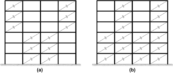

  

  Solutions in the analysis with population size equal to 30: a with four damper groups; b with six damper groups

• Conversely, increasing the number of damper groups to six (Fig. 19b), it is possible to decrease the maximum force on the structure by 25% compared with the same optimum solution.

• It is interesting to note that all solutions displayed in Table 4 are characterised by similar f₂ values, i.e. cost. In this specific case, the designer has the possibility of selecting the final solution considering a posteriori if the primary cost of the device has a higher incidence than the reinforcement intervention on the existing structure.

Considering the results of this analysis, it appears clear that the population size selected as first attempt was excessively small and by increasing this parameter more fitting solutions can be found. It must be pointed out, however, that further enlargement of the population is not allowed by the need of limiting analysis time.

Conclusions

In this paper, an optimisation tool called TOSCA, specifically designed for structural and civil engineering problems, is described. It makes use of genetic algorithms and has a general interface which can easily be adapted to external solvers without the need of programming. Along with the description of the code, a thorough discussion on the role of each GA operator is presented, with the aim of giving some indications on parameter setting and analysis assessment. Basically, the initial population should be generated by algorithms able to explore efficiently the parameter space, a problem analogous to that of experimental design. Genetic drift, a phenomenon reducing the chromosome variability in the case of small populations, may be avoided by using stochastic universal sampling as the selection algorithm. To obtain a good balance between exploration of the space and refinement of the solution, the functional specialisation hypothesis prescribes that the crossover operator should not change the population variance of the mating pool in the parameter space, while the selection operator should gradually decrease it in the objective space.

Two examples are presented. The first example is the minimisation of an analytical function of ten variables (Rastrigin function). The large number of local optima makes it ideal to test the ability of GA to reach convergence without being trapped in the local minima. The importance of tuning scaling pressure according to the crossover type utilised and of applying the mutation operator is shown. Even though the algorithm is not able to reach the real optimum, very good near-optimal solutions may be found by selecting the GA parameters according to the strategy presented above.

The second example concerns the optimal design of a seismic retrofitting system composed of nonlinear dampers for RC frames. It is shown how the design problem may be formulated as a multi-objective constrained optimisation problem. It is a mixed-integer optimisation problem, since some binary variables are used to model yes/no decisions, i.e. whether apply the damper or not. From the point of view of genetic algorithms, the presence of constraints, integer variables and multiple objectives can be easily handled. The results show the effectiveness of the approach, which is able to find solutions remarkably decreasing the interstorey drifts (which did not satisfy the standard prescription for the bare frame), but minimising different cost items. It is shown that by increasing the population size, a more fitting solution may be found, but this approach is necessarily limited by the computational effort needed by a single analysis.

References

Amadio C, Fragiacomo M, Lucia P, Luca OD (2008) Optimized design of a steel-glass parabolic vault using evolutionary multi-objective agorithms. Int J Space Struct 23(1):21–33
Baker JE (1987) Reducing bias and inefficiency in the selection algorithm. Hillsdale, New Jersey, pp 14–21
Bedon C, Morassi A (2014) Dynamic testing and parameter identification of a base-isolated bridge. Eng Struct 60:85–99
Beyer H-G, Schwefel H-P (2002) Evolution strategies—a comprehensive introduction. Nat Comput 1(1):3–52
Box MJ, Swann WH, Davies D (1969) Non-linear optimization techniques. Oliver and Boyd, Edinburgh
Byrd RH, Schnabel RB, Shultz GA (1987) A trust region algorithm for nonlinearly constrained optimization. SIAM J Numer Anal 24(5):1152–1170
EN 1998-1-1 (2005) Eurocode 8: Design of structures for earthquake resistance-Part 1: General rules, seismic actions and rules for buildings. European Standard, Brussels
Chisari C (2015) Inverse techniques for model identification of masonry structures. University of Trieste: PhD thesis
Chisari C, Bedon C (2016) Multi-objective optimization of FRP jackets for improving seismic response of reinforced concrete frames. Am J Eng Appl Sci 9(3):669–679
Chisari C, Bedon C, Amadio C (2015) Dynamic and static identification of base-isolated bridges using genetic algorithms. Eng Struct 102:80–92
Chisari C, Macorini L, Amadio C, Izzuddin BA (2016) Optimal sensor placement for structural parameter identification. Struct Multidiscip Optim 55(2):647–662
Chisari C et al (2017) Critical issues in parameter calibration of cyclic models for steel members. Eng Struct 132:123–138
Dantzig GB, Thapa MN (1997) Linear programming 1: introduction. Springer, Berlin
Dassault Systemes (2009) ABAQUS 6.9 Documentation. Providence, RI: s.n
Deb K, Pratap A, Agarwal S, Meyarivan T (2002) A fast and elitist multiobjective genetic algorithm: NSGA-II. IEEE Trans Evol Comput 6(2):182–197
Eshelman LJ, Schaffer JD (1992) Real-coded genetic algorithms and interval schemata. Found Genet Algorithms. Morgan-Kaufman, San Mateo, pp 187–202
Farina M, Amato P (2004) A fuzzy definition of “optimality” for many-criteria optimization problems. IEEE Trans Syst Man Cybern A Syst Hum 34(3):315–326
FIP Industriale SpA (n.d.) FIP Industriale. http://www.fipindustriale.it/. Accessed 26 Oct 2018
Gen M, Cheng R (1997) Genetic algorithms & engineering design. Wiley, New York
Gen M, Cheng R (1997) Genetic algorithms and engineering design. Wiley, New York
Gibbs MS, Dandy GC, Maier HR (2008) A genetic algorithm calibration method based on convergence due to genetic drift. Inf Sci 178(14):2857–2869
Goldberg DE (1989) Genetic algorithms in search, optimization and machine learning. Addison-Wesley, Boston
Goldberg DE, Deb K (1991) A comparative analysis of selection schemes used in genetic algorithms. In: Rawlins G (ed) Foundations of genetic algorithms. Morgan Kaufmann, Los Altos, pp 69–93
Hancock PJ (1994) An empirical comparison of selection methods in evolutionary algorithms. In: Fogarty TC (ed) Evolutionary computing: AISB workshop, Leeds, U.K., April 11–13, 1994. Springer, Berlin, Heidelberg, pp 80–94
Holland JH (1975) Adaptation in natural and artificial systems An introductory analysis with applications to biology, control and artificial intelligence. The University of Michigan Press, Ann Arbor
Iervolino I, Galasso C, Cosenza E (2010) REXEL: computer aided record selection for code-based seismic structural analysis. Bull Earthq Eng 8(2):339–362
Kirkpatrick S, Gelatt CD, Vecchi MP (1983) Optimization by simulated annealing. Science 220(4598):671–680
Kita H, Yamamura M (1999) A functional specialization hypothesis for designing genetic algorithms. In: Tokyo, systems, man, and cybernetics, 1999. IEEE SMC’99 conference proceedings, pp 579–584
Krishnakumar K (1990) Micro-genetic algorithms for stationary and non-stationary function optimization. In: Proceedings of the SPIE 1196, Intelligent Control and Adaptive Systems. 1989 Advances in Intelligent Robotics Systems Conference, pp 289–296
Lucia P (2008) Progettazione ottimale di ponti in struttura mista acciaio-calcestruzzo ad asse rettilineo mediante algoritmi evolutivi. Università degli studi di Trieste: PhD thesis
Mahinthakumar G, Sayeed M (2005) Hybrid genetic algorithm—local search methods for solving groundwater source identification inverse problems. J Water Resour Plan Manag 131:45–57
Mezura-Montes E, Coello Coello CA (2011) Constraint-handling in nature-inspired numerical optimization: past, present and future. Swarm Evol Comput 1(4):173–194
Michalewicz Z (1994) Genetic algorithms + data structures = evolution programs. Springer, Berlin, Heidelberg
Michalewicz Z, Logan T, Swaminathan S (1994) Evolutionary operations for continuous convex parameter spaces. World Scientific, River Edge, pp 84–97
Miettinen K (1999) Nonlinear Multiobjective Optimization. Springer, US
Mohamed AW (2017) Solving large-scale global optimization problems using enhanced adaptive differential evolution algorithm. Complex Intell Syst 3(4):205–231
Poh’sie G et al (2016a) Application of a translational tuned mass damper designed by means of genetic algorithms on a multistory cross-laminated timber building. J Struct Eng 142(4):E4015008
Poh’sie G et al (2016b) Optimal design of tuned mass dampers for a multi-storey cross laminated timber building against seismic loads. Earthq Eng Struct Dynam 45(12):1977–1995
Razali NM, Geraghty J (2011) Genetic algorithm performance with different selection strategies in solving TSP. In: Proceedings od the World Congress on Engineering, London
Ribeiro CC, Rosseti I, Souza RC (2011) Effective probabilistic stopping rules for randomized metaheuristics: GRASP implementations. In: Coello-Coello CA (ed) Learning and intelligent optimization: 5th international conference, LION 5, Rome, Italy, January 17–21, 2011. Springer, Berlin, Heidelberg
Rogers A, Prugel-Bennett A (1999) Genetic drift in genetic algorithm selection schemes. IEEE Trans Evol Comput 3(4):298–303
Sánchez AM, Lozano M, Villar P, Herrera F (2009) Hybrid crossover operators with multiple descendents for real-coded genetic algorithms: combining neighborhood-based crossover operators. Int J Intell Syst 24(5):540–567
Sloan I, Woźniakowski H (1998) When are quasi-Monte Carlo algorithms efficient for high dimensional integrals? J of Complex 14(1):1–33
Sobol I (1967) Distribution of points in a cube and approximate evaluation of integrals. USSR Comput Maths Math Phys 7:86–112
Someya H (2008) Theoretical parameter value for appropriate population variance of the distribution of children in real-coded GA. s.l. In: IEEE, pp 2717–2724
Someya H (2011) Theoretical analysis of phenotypic diversity in real-valued evolutionary algorithms with more-than-one-element replacement. Evol Comput IEEE Trans 15(2):248–266
Someya H (2012) Theoretical basis of parameter tuning for finding optima near the boundaries of search spaces in real-coded genetic algorithms. Soft Comput 16(1):23–45
Sörensen K, Glover F (2013) Metaheuristics. In: Gass SI, Fu MC (eds) Encyclopedia of operations research and management science. Springer, US, p 1641
Srinivas M, Patnaik LM (1994) Genetic algorithms: a survey. Computer 27(6):17–26
Vapnyarskii I (1994) Lagrange multipliers. In: Hazewinkel M (ed) Encyclopaedia of mathematics (Set). Encyclopaedia of mathematics. Springer, Netherlands. https://www.springer.com/cn/book/9781556080104
Wolpert DH, Macready WG (1997) No free lunch theorems for optimization. IEEE Trans Evol Comput 1(1):67–82
Zamparo R (2009) Realizzazione di un codice per la progettazione assistita di impalcati da ponte in struttura mista acciaio-calcestruzzo. Università degli studi di Trieste: PhD thesis
Zavala GR, Nebro AJ, Luna F, Coello Coello CA (2014) A survey of multi-objective metaheuristics applied to structural optimization. Struct Multidisc Optim 49(4):537–558
Zou X, Teng J, Lorenzis LD, Xia S (2007) Optimal performance-based design of FRP jackets for seismic retrofit of reinforced concrete frames. Compos B Eng 38:584–597
Acknowledgements
The authors wish to thank Mr. Enrico Parcianello for his collaboration in the second numerical example reported in this paper.
Author information
Authors and Affiliations
Corresponding author
Additional information
Publisher's Note
Springer Nature remains neutral with regard to jurisdictional claims in published maps and institutional affiliations.
Rights and permissions
Open Access This article is distributed under the terms of the Creative Commons Attribution 4.0 International License (http://creativecommons.org/licenses/by/4.0/), which permits unrestricted use, distribution, and reproduction in any medium, provided you give appropriate credit to the original author(s) and the source, provide a link to the Creative Commons license, and indicate if changes were made.
About this article
Cite this article
Chisari, C., Amadio, C. TOSCA: a Tool for Optimisation in Structural and Civil engineering Analyses. Int J Adv Struct Eng 10, 401–419 (2018). https://doi.org/10.1007/s40091-018-0205-1
Received:
Accepted:
Published:
Issue Date:
DOI: https://doi.org/10.1007/s40091-018-0205-1