Massey products in differential cohomology via stacks

Abstract

We extend Massey products from cohomology to differential cohomology via stacks, organizing and generalizing existing constructions in Deligne cohomology. We study the properties and show how they are related to more classical Massey products in de Rham, singular, and Deligne cohomology. The setting and the algebraic machinery via stacks allow for computations and make the construction well-suited for applications. We illustrate with several examples from differential geometry and mathematical physics.

1 Introduction

Massey products were introduced in [37] and further developed and generalized in [34, 38]. The existence of (higher) Massey products indicates the complexity of the topology of a space. They also determine whether and how various characterizing properties of a space might be related, in particular how homotopy of a space might be related to its cohomology [32]. On the one hand, Massey products can be viewed as secondary cohomology operations associated with the primary operation given by the cup product. On the other hand, they can also be seen as higher order products in homotopy ($A_\infty$) algebras (see [5, 51]).

A differential graded algebra (DGA) is a (not a priori commutative) graded algebra A with a map $d:A\rightarrow A$ of degree $+1$ which satisfies the relations (up to sign conventions) $dd=0$ and $d(ab)= (da)b +(-1)^{\dim a}a(db)$. Then the cohomology H(A) of A with respect to d is a graded algebra. It has further certain operations called (matrix) Massey products, the simplest of which is a correspondence

$$\begin{aligned} H(A)\otimes H(A)\otimes H(A) \rightarrow H(A), \end{aligned}$$

(1.1)

which is denoted by $\langle a,b,c\rangle$, where $a,b,c\in H(A)$. This has dimension $\dim (a)+\dim (b)+\dim (c)-1$, is defined only when $ab=bc=0\in H(A)$, and is not well-defined but rather only defined modulo terms of the form $ax +yb$ where x and y are some (auxiliary) elements of H(A). The indeterminacy may, however, sometimes be excluded, for example for dimension reasons, which occurs in applications. Generally, we have $ab=dy$ and $bc=dz$ for $y,z\in A$, so that

$$\begin{aligned} \langle a,b,c \rangle = yc + (-1)^{\dim a + 1}az, \end{aligned}$$

(1.2)

is a cocycle, with the cohomology class defined modulo the indeterminacy given above.

There are other notions of Massey products, but all are essentially variations on this principle. If the Massey product $\langle a_1,....,a_n \rangle$ exists, then all “lower” Massey products necessarily vanish, although the converse is not true in general. One may also apply a similar construction for matrices of elements, leading to matric Massey products [38], where notions related to formal flatness of the connection become important.

Differential cohomology has played an important role recently by combining geometric and topological data, namely usual cohomology and differential forms, in a coherent way [2, 7, 9, 10, 12, 17, 22, 27, 33, 50, 53]. It is natural then to try to extend Massey products, which exist in both of these ingredients, to differential cohomology. Massey products have been considered in Deligne cohomology in [19, 41, 49, 55]. We extend the definitions and constructions to the level of stacks,¹ which has the virtue of allowing for vast generalization to various settings and to a plethora of applications. We believe this formulation has an advantage both for theory and for applications. In particular, we emphasize that desired properties and behaviour of the Massey products are clearer and systematic in stacks, and computations are generally doable and are more efficient there, making them quite suitable for applications. The constructions are based on the thesis [31], but we have taken the opportunity here to sharpen the results and add properties and applications. We emphasize that this paper is the first part of a bigger project, aimed at developing various concrete computational techniques for differential cohomology theories.

The paper is organized as follows. In Sect. 2, we provide the setting for the two main ingredients that we would like to combine, namely classical (generalized) Massey products in Sect. 2.1 and differential cohomology in Sect. 2.2. We set up the former in the general framework of [1, 34, 38] and the latter in the language of stacks (see [25, 47, 53]). Then we recall the Deligne–Beilinson cup product in differential cohomology, as set forth in [23, 24], in Sect. 2.3. The first encounter of Massey products in differential cohomology in the particular setting of Deligne cohomology is recalled in Sect. 2.4 and adapted slightly to our language. Our main construction is then described in Sect. 3, where we first set up the powerful machinery needed, in the form of the Dold–Kan correspondence, in Sect. 3.1, and then provide the main definitions in Sect. 3.2. Part of this construction, together with a lot of the homotopic background appeared in the second author’s thesis [31]. A vast generalization, along the lines of the classic work of May, is presented in Sect. 3.3, where we present all three of differential, singular, and de Rham Massey products within the same setting. Then in Sect. 3.4 we give the properties of the Massey products thus defined. These turn out to be rather attractive in general, with some unexpected features.

In Sect. 4, we illustrate (some aspects of) the construction with various applications. We will first give instances of where the classical Massey products arise in applications, and we apply our constructions in previous sections to supply the differential refinements of these applications. We extend the constructions and discussion in [23] from cup product Chern–Simons theories to what we might call Massey product Chern–Simons theories. In Sect. 4.1, we illustrate how (stacky) Massey products arise in trivialization of higher structures, such as (differential) String, Fivebrane [46], and Ninebrane structures [45]. This gives natural trivializations of Chern–Simons theories at the level of (higher) bundles with connections. There are two expressions that involve three differential cohomology classes, namely the stacky Massey product and the triple Deligne–Beilinson cup product. A natural question is whether these are related. Indeed, we propose such a relation via transfer in the context of cobordism.

Then, in Sect. 4.2, we see how systems arising generally in anomaly cancellation lead naturally to (stacky) Massey products. Finally, in settings inspired by type IIA and type IIB string theory in Sects. 4.3 and 4.4, respectively, we illustrate how these lead to stacky Massey products. Interestingly, the latter gives rise to a quadruple Massey product. The reader need not be familiar with these string theories in order to follow the discussion.

2 Massey products and differential cohomology

2.1 Classical (generalized) Massey products

We recall some notions from [1, 34, 38]. This will be useful for the applications that we will consider later as well as a starting point for comparison with our stacky constructions.

Let $({\mathcal {A}},d)$ be a differential graded algebra over $\mathbb {R}$ endowed with augmentation. Let $M(\mathcal {A})$ be the set of all upper triangular half-infinite matrices with entries in $\mathcal {A}$, zeroes on the diagonal and finitely many nonzero entries, i.e.

$$\begin{aligned} M(\mathcal {A})= & {} \left\{ A=(a_{ij}), a_{ij}\in \mathcal {A}, a_{ij}=0 ~\mathrm{for}~ j\le i~ \mathrm{and}~ i,j \ge n+1 \right. \nonumber \\&\left. ~\mathrm{for~ some}~ n ~\text {with}~ i, j \in \mathbb {N}\right\} . \end{aligned}$$

(2.1)

The last condition distinguishes in $M(\mathcal {A})$ a subset (which is in fact a subalgebra) $M_n(\mathcal {A})$ consisting of all $(n\times n)$-matrices with entries in $\mathcal {A}$. The algebra $M(\mathcal {A})$ is bigraded and endowed with a bigraded Lie bracket. We introduce the differential d on $M(\mathcal {A})$ as $dA=(da_{ij})_{i,j\ge 1}$. The algebra $\mathcal {A}$ admits an involution given by $a \mapsto {\overline{a}}=(-1)^k a$, which can be extended to an automorphism of $M(\mathcal {A})$ as ${\overline{A}}=(\overline{a}_{ij})_{i,j \ge 1}$, with the differential d satisfying the generalized Leibnitz rule $d(AB) = (dA)B + {\overline{A}}(dB)$. In [1], the Maurer–Cartan operator $\mu :~M(\mathcal {A}) \longrightarrow M(\mathcal {A})$ was defined as $\mu (A)=dA - {\overline{A}} \cdot A$. Then a matrix $A\in M(\mathcal {A})$ is said to be a matrix of formal connection if it satisfies the Maurer–Cartan equation in $\mathcal {A}$,

$$\begin{aligned} dA -{\overline{A}} \cdot A \equiv 0 ~~\mathrm{mod} \ker A, \end{aligned}$$

(2.2)

i.e. A is a formal connection if $\mu (A) \in \ker A$. Here $\ker A$ is a $\mathcal {A}$-module generated by matrices ${1_{ij}}$ such that $A\cdot 1_{ij}=1_{ij} \cdot A$, where $1_{ij}$ denotes the matrix that has all zero entries except for 1 as the ij-entry. Note that this implies that $AB=BA$ for any matrix $B \in \ker A$. The element $\mu (A)$ is called the curvature of the formal connection A, and can be shown to be closed (see e.g. [1, 14]).

Now comes the relation between Maurer–Cartan and Massey products. The generalized Massey products are the cohomology classes of the curvature matrices of the formal connection A, i.e. if A is a solution to the Maurer–Cartan equation then the entries of the matrix $[\mu (A)]$ are the generalized Massey products [1]. Geometrically, this means that the latter measure the deviation of connections from flat ones, so that the connection is flat if they vanish. Later we will make use of this approach in describing Massey products in stacks.

Classical Massey products in integral cohomology $H^*(X; \mathbb {Z})$ arise by taking $\mathcal {A}$ to be an algebra over the commutative ring $\mathbb {Z}$, with the multiplication being associative but not necessarily graded-commutative. Now let $\alpha , \beta , \gamma$ be the cohomology classes of closed elements $a\in \mathcal {A}^p$, $b \in \mathcal {A}^q$, and $c\in \mathcal {A}^r$. The triple Massey product $\langle \alpha , \beta , \gamma \rangle$ is defined if one can solve the Maurer–Cartan equation with the formal connection

$$\begin{aligned} A= \left( \begin{array}{c@{\quad }c@{\quad }c@{\quad }c} 0 &{} a &{} {\tilde{f}} &{} *\\ 0 &{} 0 &{} b &{} {\tilde{g}} \\ 0 &{} 0 &{} 0 &{} c \\ 0 &{} 0 &{} 0 &{} 0 \end{array} \right) . \end{aligned}$$

This is equivalent to the two separate equations

$$\begin{aligned} d{\tilde{f}} = (-1)^p a \wedge b \quad \mathrm{and} \quad d{\tilde{g}} = (-1)^q a \wedge c , \end{aligned}$$

(2.3)

and that implies that the Massey product is defined if and only if

$$\begin{aligned} \alpha \cup \beta = \beta \cup \gamma =0 \in H^*(\mathcal {A}). \end{aligned}$$

(2.4)

The matrix $\mu (A)$ has the form

$$\begin{aligned} \mu (A)=dA- {\overline{A}} \cdot A= \left( \begin{array}{c@{\quad }c@{\quad }c@{\quad }c} 0 &{} 0 &{} 0 &{} \tau \\ 0 &{} 0 &{} 0 &{} 0 \\ 0 &{} 0 &{} 0 &{} 0 \\ 0 &{} 0 &{} 0 &{} 0 \end{array} \right) \end{aligned}$$

and defines the Massey product $[\mu (A)]$ which is equal to the cohomology class

$$\begin{aligned} \langle \alpha , \beta , \gamma \rangle = [\tau ]= \left[ (-1)^{p+1} a \wedge {\tilde{g}} + (-1)^{p+q}{\tilde{f}} \wedge c \right] . \end{aligned}$$

(2.5)

Here $[a] \in H^*(\mathcal {A})$ denotes the cohomology class of a closed element $a \in \mathcal {A}$, and $[A]=([a_{ij}])_{i, j \ge 1}\in M(H^*(\mathcal {A})$, for a closed matrix $A \in M(\mathcal {A})$, denotes the corresponding matrix whose entries are the cohomology classes of the entries $a_{ij}$ of A. Since ${\tilde{f}}$ and ${\tilde{g}}$ are defined by expressions (2.3) up to closed elements from $\mathcal {A}$, the triple Massey product $\langle \alpha , \beta , \gamma \rangle$ is defined modulo $\alpha \cdot H^{q+r}(\mathcal {A}) + \gamma \cdot H^{p+q}(\mathcal {A})$.

2.2 Differential cohomology

There are several different approaches to differential cohomology. Initially, we will be concerned with the construction as Deligne cohomology [7, 27]. We will then move to the stacky setting, which illuminates the true nature of differential cohomology as a theory which counts isomorphism classes of higher U(1)-gerbes with connection (generalizing the usual discussion for the gerbe case in [7]).

The classical construction relies on hypercohomology of a complex of objects of an abelian category as an extension to complexes of the usual cohomology of an object. For $n\in \mathbb {N}$, let $\mathbb {Z}^\infty _{\mathcal {D}}[n]$ be the sheaf of chain complexes given by

$$\begin{aligned} \mathbb {Z}^\infty _\mathcal {D}[n]:=[\cdots \rightarrow 0 \rightarrow \underline{\mathbb {Z}} \hookrightarrow \Omega ^{0} \rightarrow \Omega ^{1} \rightarrow \cdots \rightarrow \Omega ^{n-1}], \end{aligned}$$

where $\underline{\mathbb {Z}}$ is in degree² n and $\Omega ^{n-1}$ is the sheaf of real-valued $(n-1)$-forms in degree 0. Given a manifold X, the degree n sheaf hypercohomology with coefficients in $\mathbb {Z}^\infty _\mathcal {D}[n]$ can be defined to be the degree n differential cohomology of X:

$$\begin{aligned} \widehat{H}^{n}(X;\mathbb {Z}):=H^{n}(X; \mathbb {Z}^\infty _{\mathcal {D}}[n]). \end{aligned}$$

(2.6)

If X is paracompact, then these cohomology groups are given by the cohomology of the total complex of the Čech–Deligne double complex corresponding to a good open cover of X. In what follows, we will always assume that X is paracompact, so that the hypercohomology groups can be computed by either taking arbitrary injective resolutions, or via this more explicit Čech approach.

In [50] (see also [9]), it was observed that these cohomology groups fit nicely into an exact hexagon

where the bottom row is the Bockstein sequence and the diagonals are exact. The map R is called the curvature map and I is called the integration map. Notice that, by exactness, in the case that the curvature of a differential cohomology class vanishes, the class lies in the image of the inclusion $H^{n-1}(X;U(1))\hookrightarrow \widehat{H}^{n}(X;\mathbb {Z})$. We call these classes flat, as they represent n-gerbes with connections of vanishing curvature. Differential cohomology therefore detects the topological information—when the class is flat—and the differential geometric information encoded by the curvature. See [2, 7, 10, 12, 17, 22, 27, 33, 50, 53] for more details on the various approaches.

As we mentioned earlier, our point of view henceforth will be mainly that of stacks. We will recall and introduce some stacks that will be useful for us. We start by surveying some basic concepts and definitions from [23,24,25, 36], adapted to our setting. We will provide only as much detail as necessary to introduce our stacks.

For $n \in \mathbb {N}$, let $\mathscr {C}\mathrm {art}\mathscr {S}\mathrm {p}$ be the category with objects convex open subsets of Cartesian space $\mathbb {R}^{n}$ (hence diffeomorphic to $\mathbb {R}^n$), and morphisms smooth functions. A smooth prestack is simply a functor

$$\begin{aligned} \mathcal {F}:\mathscr {C}\mathrm {art}\mathscr {S}\mathrm {p}^\mathrm{op}\rightarrow s\mathscr {S}\mathrm {et}\end{aligned}$$

with target the category of simplicial sets. The passage from prestacks to stacks is achieved by imposing a sort of gluing condition on $\mathcal {F}$. Roughly speaking, a stack $\mathcal {F}$ attaches an entire space (equivalently simplicial set) of data to each object in $\mathscr {C}\mathrm {art}\mathscr {S}\mathrm {p}$. This data should be viewed as being local data. The gluing condition then assembles this data into a geometric object, which is a stack. More precisely, we say that a prestack $\mathcal {F}$ satisfies descent if for each $U\in \mathscr {C}\mathrm {art}\mathscr {S}\mathrm {p}$ and each open cover $\{U_{i}\}_{i\in I}$ of U with contractible finite intersections $U_{i_1i_2\ldots i_k}$, we have a weak equivalence

In particular, if $\mathcal {F}$ takes values in Kan complexes, this weak equivalence is part of an actual homotopy equivalence. The reader may notice the following.

• If we change the target category to $\mathscr {S}\mathrm {et}$ and impose the stronger condition that the strict limit over the diagram was isomorphic to $\mathcal {F}(U)$, we would recover the gluing condition for a sheaf.

• If we change the target category to groupoids, then the above condition recovers the usual notion of descent for classical stacks.

In the latter, homotopy equivalence is simply categorical equivalence of groupoids. Hence the gluing condition respects the correct notion of equivalence (which is weaker than isomorphism). We can therefore view the equivalence (2.8) as the more general gluing condition for $\infty$-groupoids (or Kan complexes). We need the following (see [21, 36, 53]).

Definition 1

We call a smooth prestack $\mathcal {F}$ a smooth stack if it satisfies descent. We denote the full subcategory of smooth stacks by

$$\begin{aligned} \mathscr {S}\mathrm {h}_{\infty }(\mathscr {C}\mathrm {art}\mathscr {S}\mathrm {p})\hookrightarrow [\mathscr {C}\mathrm {art}\mathscr {S}\mathrm {p}^\mathrm{op},s\mathscr {S}\mathrm {et}], \end{aligned}$$

where the brackets denote the category of contravariant functors from $\mathscr {C}\mathrm {art}\mathscr {S}\mathrm {p}$ to $s\mathscr {S}\mathrm {et}$, with morphisms that are natural transformations.

Note that the above functor category is simplicially enriched in a natural way. Observe that for objects X and Y in any (locally small) category, $\mathrm{hom}(X, Y)$ is always a set. This allows us to form the mapping space (i.e. simplicial set), which at level n is

$$\begin{aligned} \big (\text {Map}(X, Y) \big )_n:=\text {hom}\big (X \times \underline{\Delta [n]}, Y\big ), \end{aligned}$$

when X is fibrant and Y cofibrant (this requires a model structure). Here the operation $\times$ is the Cartesian product in stacks, and the underline on $\Delta [n]$ denotes taking the locally constant stack associated to $\Delta [n]$.

Remark 1

The inclusion functor admits a left adjoint L which preserves homotopy colimits (in fact, a left Quillen adjoint [53]). We call this functor L the stackification functor and call the image of a prestack $\mathcal {F}$ under L the stackification of $\mathcal {F}$.

In [25], the moduli stack of n-gerbes with connection, $\mathbb {B}^{n} U(1)_\mathrm{conn}$, was introduced. This stack was obtained as the stackification of the n-prestack obtained by applying the Dold–Kan map (see Sect. 3.1) to the Deligne presheaf of chain complexes

$$\begin{aligned} \mathbb {Z}^{\infty }_{\mathcal {D}}[n+1]:=[\cdots \rightarrow 0 \rightarrow \underline{\mathbb {Z}} \hookrightarrow \Omega ^{1} \rightarrow \Omega ^{2} \rightarrow \cdots \rightarrow \Omega ^{n}]. \end{aligned}$$

These stacks are the differential analogues of Eilenberg-MacLane spaces and, for a fixed manifold X, there is a bijective correspondence (a “representation”)

$$\begin{aligned} \widehat{H}_{\mathcal {D}}^{n+1}(X;\mathbb {Z})\simeq \pi _0\mathrm {Map}(X,\mathbb {B}^{n} U(1)_\mathrm{conn}), \end{aligned}$$

(2.9)

where the right hand side is the set of morphisms in the homotopy category of stacks.

Remark 2

In general the right hand side of the correspondence (2.9) may not be well-defined. In order to be able to take homotopy groups of the mapping space $Y:=\mathrm {Map}(X,\mathbb {B}^{n} U(1)_\mathrm{conn})$, Y has to be a Kan complex, which is the case when X is confibrant and $\mathbb {B}^{n} U(1)_\mathrm{conn}$ is fibrant. However, since $\mathbb {B}^{n}U(1)_\mathrm{conn}$ satisfies descent, it is fibrant in a particular local model structure on presheaves (see [25]). Even though X can be viewed as a stack, it is not cofibrant, and so we need to cofibrantly replace it. Indeed, if X is a (paracompact) manifold, thought of as a smooth stack, with good open cover $\{U_{i}\}_{i\in I}$, then we can replace X by its Čech nerve

which is both cofibrant and weak equivalent to X in the category of smooth stacks $\mathrm{Sh}_\infty (\mathscr {C}\mathrm {art}\mathscr {S}\mathrm {p})$ [20]. For purely model category theoretic reasons it then follows that $\mathrm {Map}(C(\{U_{i}\}),\mathbb {B}^{n}U(1)_\mathrm{conn})$ is a Kan complex and we can take $\pi _{0}$, obtaining the set of morphisms in the homotopy category. This motivates the definition

$$\begin{aligned} \mathrm {Map}(X,\mathbb {B}^{n}U(1)_\mathrm{conn}):=\mathrm {Map}(C(\{U_{i}\}),\mathbb {B}^{n}U(1)_\mathrm{conn}). \end{aligned}$$

As explained in [25], these stacks also have a nice geometric interpretation. The following example illustrates the point quite well.

Example 1

Let X be a manifold. Let us calculate the set of vertices of the mapping space $\mathrm {Map}(X,\mathbb {B}^{2}U(1)_\mathrm{conn})$. Using the pointwise formula for the homotopy colimit [25], we have

$$\begin{aligned} \hom (X,\mathbb {B}^{2}U(1)_\mathrm{conn})= & {} \hom (C(\{U_{i}\}),\mathbb {B}^2U(1)_\mathrm{conn})\nonumber \\= & {} \hom \Big (\int ^{k\in \Delta }\underline{\Delta [k]}\times \coprod _{\alpha _{1},..,\alpha _{k}}U_{\alpha _{1},..,\alpha _{k}},~\mathbb {B}^{2}U(1)_\mathrm{conn}\Big )\nonumber \\= & {} \int _{k\in \Delta }\prod _{\alpha _{1},..,\alpha _{k}}\hom (\underline{\Delta [k]}\times U_{\alpha _{1},..,\alpha _{k}},~\mathbb {B}^{2}U(1)_\mathrm{conn})\nonumber \\= & {} \prod _{\alpha _{1},..,\alpha _{k}}\int _{k\in \Delta }\hom \big (\underline{\Delta [k]},~\mathbb {B}^{2}U(1)_\mathrm{conn}(U_{\alpha _{1},..,\alpha _{k}})\big ).\qquad \end{aligned}$$

(2.11)

An element of the hom in the last line can be written out explicitly as a choice maps

$$\begin{aligned} B_{\alpha }&:\Delta [0]\rightarrow \prod _{\alpha }\mathbb {B}^{2}U(1)(U_{\alpha }) \nonumber \\ A_{\alpha \beta }&: \Delta [1]\rightarrow \prod _{\alpha \beta }\mathbb {B}^{2}U(1)(U_{\alpha \beta }) \nonumber \\ g_{\alpha \beta \gamma }&: \Delta [2] \rightarrow \prod _{\alpha \beta \gamma }\mathbb {B}^{2}U(1)(U_{\alpha \beta \gamma }), \end{aligned}$$

(2.12)

such that the face inclusions of each map are equal to their corresponding restrictions to higher intersections. Now since equivalent stacks will produce the same cohomology groups, we do not distinguish between equivalent stacks. In particular, using the exponential quasi-isomorphism, we could have equivalently defined $\mathbb {B}^{2}U(1)_\mathrm{conn}$ to be the stackification of the prestack given by applying the Dold–Kan functor to the presheaf of chain complexes

$$\begin{aligned}{}[ 0 \rightarrow \cdots \rightarrow C^{\infty }(-,U(1)) \overset{d\log }{\longrightarrow } \Omega ^{1} \rightarrow \Omega ^{2}]. \end{aligned}$$

We can therefore describe the choices of $B_{\alpha }$,$A_{\alpha \beta }$ and $g_{{\alpha \beta \gamma }}$ via the 2-simplex.

Here, $g_{\alpha \beta \gamma }$ is a choice of smooth U(1)-valued function on triple intersections, $A_{\alpha \beta }$ is a choice of 1-form on double intersections and $B_{\alpha }$ is a choice of 2-form on open sets. Moreover, we have that these assignments must satisfy the conditions

• (i) $g_{\alpha \beta }~g_{\gamma \beta }^{-1}~g_{\gamma \alpha }=1$;

• (ii) $g_{\alpha \beta \gamma }^{-1}~dg_{\alpha \beta \gamma }=d\log (g)_{\alpha \beta \gamma }=A_{\alpha \beta }-A_{\gamma \beta }+A_{\gamma \alpha }$;

• (iii) $B_{\beta }-B_{\alpha }=dA_{\alpha \beta }$.

We identify this data as precisely giving a gerbe with connection [7]. Moreover, the fact that $\mathbb {B}^{n}U(1)_\mathrm{conn}$ is a stack ensures that $F_{\alpha }=dB_{\alpha }$ is a globally defined 3-form: the curvature of the gerbe. Notice that these are only the vertices in the mapping space. The entire mapping space keeps track of more information, namely the homotopies and higher homotopies between gerbes. These encode automorphisms in the sense of gauge transformations (see [23, 24]).

Example 2

Let X be a paracompact manifold and $C(\{U_i\})$ the Čech nerve of some good open cover. The maps

$$\begin{aligned} L:C(\{U_i\})\rightarrow \mathbb {B}U(1)_\mathrm{conn} \end{aligned}$$

are in bijective correspondence with circle bundles on X equipped with a connection. In fact, using the calculations in the above example shows that such a morphism gives the data U(1)-valued functions $g_{\alpha \beta }$ on intersections satisfying $g_{\alpha \beta }g_{\beta \gamma }^{-1}g_{\gamma \delta }=1$ on triple intersections, along with 1-forms $A_{\alpha }$ on open sets satisfying $A_{\alpha }-A_{\beta }=d\log (g)_{\alpha \beta }$ on double intersections. If the homotopy class of L is trivial, then the circle bundle is trivializable. In fact, the trivializing map $\phi$ is nothing but a homotopy $\phi :L \rightarrow 0$. To identify this homotopy, we use the Dold–Kan correspondence. In particular, an edge in $\mathrm {Map}(C(\{U_i\}),\mathbb {B}U(1)_\mathrm{conn})$ is, by adjunction, an edge in the simplicial set

$$\begin{aligned} \mathrm {Map}(C(\{U_i\}),\mathbb {B}^{n}U(1)_\mathrm{conn})=\mathrm{DK}(\hom _{\mathscr {C}\mathrm {h}^{+}}(N(C(\{U_i\})),\mathbb {Z}^{\infty }_{\mathcal {D}}[2])), \end{aligned}$$

(2.13)

where N is the normalized Moore functor. Recall that this functor gives an equivalence of categories, from simplicial abelian groups $s\mathscr {A}\mathrm {b}$ to chain complexes in non-negative degrees $\mathrm{Ch}_\bullet ^+$ (see [28]). The hom in positively graded chain complexes is the truncated total complex of the Čech–Deligne double complex

$$\begin{aligned} \left[ \cdots \rightarrow \mathrm {tot}^{1}C(\mathcal {U},\mathbb {Z}^{\infty }_{\mathcal {D}}[2]) \rightarrow Z\left( \mathrm {tot}^{2}C(\mathcal {U},\mathbb {Z}^{\infty }_{\mathcal {D}}[2])\right) \right] , \end{aligned}$$

where Z denotes the group of cocycles in that degree. Recalling that the differential is given by $D:=d+(-1)^{k}\delta$, where $\delta$ takes the alternating sum of restrictions, we identify an edge connecting L and 0 as an assignment of Čech–Deligne cochain h of degree 1 such that $(d-\delta )h=L$. Explicitly, this means a choice of U(1)-valued function $h_{\alpha }$ on open sets such that

• (i) $h_{\alpha }h_{\beta }^{-1}=g_{\alpha \beta }$;

• (ii) $-ih_{\alpha }^{-1}dh_{\alpha }=d\log (h_{\alpha })=A_{\alpha }$.

A straightforward calculation shows that the pattern continues and that null homotopies of n-gerbes (equivalently n-bundles, equivalently maps into $\mathbb {B}^{n}U(1)_\mathrm{conn}$) can again be identified with trivializations.

Motivated by this last example, we will often refer to null homotopies as trivializations. To summarize, the mapping space $\mathrm {Map}(X,\mathbb {B}^{n}U(1)_\mathrm{conn})$ can be identified with the set of all n-gerbes with connection, along with isomorphisms between these and higher homotopies between these isomorphisms.

Remark 3

There are several other stacks related to $\mathbb {B}^{n}U(1)_\mathrm{conn}$ which are useful for us and are defined as follows (see [23,24,25, 53]):

• (i) If we forget about the connection on the these n-bundles, we obtain the bare moduli stack of n-gerbes $\mathbb {B}^{n}U(1)$. Explicitly, this stack is obtained by applying the Dold–Kan functor to the sheaf of chain complexes $C^{\infty }(-,U(1))[n]$: the sheaf of smooth U(1)-valued functions in degree n.

• (ii) We also define a stack which represents flat n-bundles with connection, $\flat \mathbb {B}^{n}U(1)$. This stack is obtained by applying Dold–Kan to the sheaf of chain complexes $\mathrm{disc}{U(1)}[n]$: the sheaf of locally constant U(1) valued functions in degree n.³

• (iii) We have a stack representing the truncated de Rham complex $\flat _\mathrm{dR}\mathbb {B}^{n}U(1)$ obtained by applying Dold–Kan to the truncated de Rham sheaf of chain complexes

  $$\begin{aligned} \Omega ^{\le n}_\mathrm{cl}:=[\cdots 0 \rightarrow \Omega ^{0}\rightarrow \Omega ^{1} \rightarrow \cdots \rightarrow \Omega ^{n}_\mathrm{cl}]. \end{aligned}$$

• (iv) Finally, we define the stack of closed n-forms $\Omega ^{n}_\mathrm{cl}$ to be the stack obtained by applying Dold–Kan to the sheaf of closed n-forms.

One way to see that the second stack really does detect flat n-gerbes with connection is to observe that, by Poincaré lemma, one has a quasi-isomorphism of sheaves

$$\begin{aligned} \mathrm{disc}(U(1))[n]\simeq [ 0 \rightarrow \cdots \rightarrow C^{\infty }(-,U(1)) \overset{d\log }{\longrightarrow } \Omega ^{1} \rightarrow \cdots \rightarrow \Omega ^{n}_\mathrm{cl}], \end{aligned}$$

where on the right we have closed n-forms in degree 0. These n-forms are to be interpreted as giving the connection on the corresponding bundle. Hence, if the form is closed then the bundle is flat.

The moduli stack $\mathbb {B}^{n}U(1)_\mathrm{conn}$ is related to the stacks in Remark 3 in various ways. In [25, 53], it was observed that $\mathbb {B}^{n}U(1)_\mathrm{conn}$ is the homotopy pullback

(2.14)

where the left composite $\mathbb {B}^{n}U(1)_\mathrm{conn}\rightarrow \mathbb {B}^{n}U(1)\overset{\theta }{\rightarrow } \flat _\mathrm{dR}\mathbb {B}^{n+1}U(1)$ is homotopic to the map

$$\begin{aligned} \mathrm{curv}:\mathbb {B}^{n}U(1)_\mathrm{conn}\rightarrow \flat _\mathrm{dR}\mathbb {B}^{n+1}U(1), \end{aligned}$$

(2.15)

induced by the morphism of sheaves of chain complexes

(2.16)

This map gives the full de Rham data for the curvature of a bundle with connection. In fact, if one calculates the sheaf hypercohomology in degree 0 of the bottom row, say via the Čech-de Rham complex (as in [6]), one gets $H^{n}_\mathrm{dR}(X)$. Consequently, the map $\mathrm{curv}$ induces a map

$$\begin{aligned} \mathrm{curv}_*:\pi _{0}\mathrm {Map}(X,\mathbb {B}^{n}U(1)_\mathrm{conn})\longrightarrow H^{n+1}_\mathrm{dR}(X), \end{aligned}$$

(2.17)

which sends an $(n-1)$-gerbe with connection to the de Rham class of its curvature. The following proposition might certainly be known to experts, but we include a proof for completeness.

Lemma 2

The homotopy fiber of the map

$$\begin{aligned} R:\mathbb {B}^{n}U(1)_\mathrm{conn}\twoheadrightarrow \Omega ^{n+1}_\mathrm{cl}, \end{aligned}$$

can be identified with $\flat \mathbb {B}^{n}U(1)$.

Proof

The map R is induced by the morphism of sheaves of chain complexes

(2.18)

Since this map is degree-wise surjective by Poincaré lemma (traditionally in highest form-degree, and trivially in lower degrees), it is a fibration in the projective model structure on presheaves of chain complexes. We can therefore calculate the homotopy fiber as the kernel of that map. By inspection, the kernel is

$$\begin{aligned}{}[\cdots \rightarrow \underline{\mathbb {Z}} \hookrightarrow \Omega ^{0}\rightarrow \Omega ^{1} \rightarrow \cdots \rightarrow \Omega ^{n}_\mathrm{cl}], \end{aligned}$$

which, via the exponential map, is quasi-isomorphic to

$$\begin{aligned}{}[\cdots C^{\infty }(-,U(1))\overset{d \mathrm{log}}{\longrightarrow } \Omega ^{1}\rightarrow \cdots \rightarrow \Omega ^{n}_\mathrm{cl}]. \end{aligned}$$

Again, by Poincaré lemma, this sheaf of chain complex is quasi-isomorphic to $\mathrm{disc}(U(1))[n].$ Since the Dold–Kan functor is a right Quillen adjoint and preserves weak equivalences, it takes fibration sequences to fibration sequences and we have the desired result.$\square$

Using the above proposition along with diagram (2.14) and the pasting lemma for homotopy pullbacks, we observe that we have the following iteration of homotopy pullbacks [53]

(2.19)

where 0 is the 0 map. From Lemma 2 along with this last diagram, we immediately get the following:

Proposition 3

The based loop stack $\Omega \mathbb {B}^{n}U(1)_\mathrm{conn}$ can be identified with the stack $\flat \mathbb {B}^{n-1}U(1)$.

Proof

Consider the homotopy pullback square

within diagram (2.19). Such a homotopy pullback, given by the outer square, can be taken as a definition of the loop space. Alternatively, a homotopy pullback can be computed explicitly as the paths in $\mathbb {B}^nU(1)_\mathrm{conn}$ connecting the point inclusion $*\rightarrow \mathbb {B}^nU(1)_\mathrm{conn}$ to itself: a loop. $\square$

Note that Massey products in the homology of the based loop space is classically considered in [13, 52]. The above discussions allows us to recast the “differential cohomology diamond” using our stacks.

Proposition 4

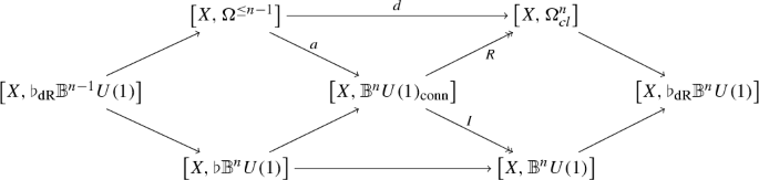
The differential cohomology diagram (2.17) lifts to a diagram of stacks

where the diagonals are fibration sequences.

Proof

This is the same diagram as a portion of diagram (2.19) rotated. The top and bottom horizontal maps in (2.20) are defined as the compositions $d=Ra$ and $\beta =jI$. Fixing a manifold X, mapping into this diagram, and passing to connected components, i.e. taking $\pi _0 \mathrm {Map}(X, -)$, we recover the diamond diagram (2.17). Note that d in (2.20) recovers the usual exterior derivative, by the nature of R, and that $\beta$ recovers the Beckstein by uniqueness of the latter as a cohomology operation. $\square$

We now explain how to go the other direction, i.e. from stacks to Deligne cohomology. We have seen that for a manifold X, the mapping space $\mathrm {Map}(X,\mathbb {B}^{n}U(1)_\mathrm{conn})$ can be identified with the space of n-gerbes equipped with connections (along with all isomorphisms and higher isomorphisms between them). It will be convenient to organize this mapping space itself into a stack. We define the mapping stack to be the stackification of the prestack given by the assignment

$$\begin{aligned} U\mapsto \mathrm {Map}(X\times U,\mathbb {B}^nU(1)_\mathrm{conn}), \end{aligned}$$

(2.21)

for each $U\in \mathscr {C}\mathrm {art}\mathscr {S}\mathrm {p}$. We denote this stack by⁴ $[X,\mathbb {B}^nU(1)_\mathrm{conn}]$.

Remark 4

Notice the following:

• (i) If we evaluate the mapping stack on the terminal object in $\mathscr {C}\mathrm {art}\mathscr {S}\mathrm {p}$ (the point) and take $\pi _0$, we recover the usual differential cohomology groups from the correspondence (2.9)

  $$\begin{aligned} \pi _0[X,\mathbb {B}^nU(1)_\mathrm{conn}](*)\simeq \pi _0\mathrm {Map}(X\times *,\mathbb {B}^nU(1)_\mathrm{conn})\simeq \widehat{H}^n(X,\mathbb {Z}). \end{aligned}$$

• (ii) Since the mapping stack is clearly functorial in both arguments and the stackification functor preserves homotopy fibers (it is left exact), we can map into the diagram (2.19) to obtain the diagram

  

  where the diagonals are again fibration sequences. If we evaluate this previous diagram at the point and apply $\pi _0$, we indeed reproduce the usual differential cohomology diamond diagram (2.17).

2.3 Cup product in differential cohomology

Deligne [16] and Beilinson [3] showed that differential cohomology admits a distinguished cup product refining the usual cup product on singular cohomology. This product is defined on sections of $\mathbb {Z}^\infty _\mathcal {D}[n]$ by the formula

$$\begin{aligned} \alpha \cup _\mathrm{DB} \beta =\left\{ \begin{array}{c@{\quad }c@{\quad }c} \alpha \beta , &{}&{} \ \mathrm {deg}(\alpha )=n \\ \alpha \wedge d\beta , &{}&{} \ \mathrm {deg}(\alpha )=0 \\ 0, &{}&{} \ \text {otherwise}. \end{array}\right. \end{aligned}$$

(2.22)

Note that the grading here is such that the first case is simply multiplication by an integer. In fact, it is obvious from the definition that the Deligne–Beilinson (henceforth DB) cup product composed with the natural inclusion

$$\begin{aligned} \underline{\mathbb {Z}}[n]\hookrightarrow \mathbb {Z}^{\infty }_{\mathcal {D}}[n], \end{aligned}$$

simply multiplies the two locally constant integer-valued functions. Since the sheaf cohomology of the locally constant sheaf $\underline{\mathbb {Z}}$, equipped with this product, is simply the ordinary cohomology ring with integral coefficients, one immediately sees that this cup product does indeed refine the usual cup product.

Equipped with this cup product, $\widehat{H}^{*}(X;\mathbb {Z})$ becomes an associative and graded-commutative ring [7]. This cup product structure also refines the wedge product of forms in the sense that the curvature map $R:\widehat{H}^{*}(X;\mathbb {Z})\rightarrow \Omega ^{*}_\mathrm{cl}$ defines a homomorphism of graded commutative rings [9]. In particular this implies that the cup product of two classes of odd degree is flat. It can also be shown [9] that the cup product of a flat class with any other class is again flat and that the inclusion of $H^*(X, U(1))$ into $\widehat{H}^*(X; \mathbb {Z})$ is a two sided ideal.

We now turn to the cup product, viewed as a morphism of stacks. In [23] it was observed that the lax monoidal structure of the Dold–Kan map gives rise to a cup product, exhibited as a morphism

$$\begin{aligned} \cup :\mathbb {B}^{m} U(1)_\mathrm{conn} \times \mathbb {B}^{n} U(1)_\mathrm{conn}\longrightarrow \mathbb {B}^{n+m+1} U(1)_\mathrm{conn}, \end{aligned}$$

(2.23)

of stacks. This map is obtained by simply taking the DB cup product (2.22)

$$\begin{aligned} \cup _\mathrm{DB}:\mathbb {Z}^{\infty }_{\mathcal {D}}[n+1]\otimes \mathbb {Z}^{\infty }_{\mathcal {D}}[m+1] \longrightarrow \mathbb {Z}^{\infty }_{\mathcal {D}}[n+m+2], \end{aligned}$$

applying the Dold–Kan map

$$\begin{aligned} \mathrm{DK}(\cup _\mathrm{DB}): \mathrm{DK}(\mathbb {Z}^{\infty }_{\mathcal {D}}[n+1]\otimes \mathbb {Z}^{\infty }_{\mathcal {D}}[m+1]) \longrightarrow \mathrm{DK}(\mathbb {Z}^{\infty }_{\mathcal {D}}[n+m+2]), \end{aligned}$$

and using the lax monoidal structure $\varphi$ of the map $\mathrm{DK}$ to get a map

$$\begin{aligned} \cup= & {} \mathrm{DK}(\cup _\mathrm{DB})\circ \varphi : \mathrm{DK}(\mathbb {Z}^{\infty }_{\mathcal {D}}[n+1]) \times \mathrm{DK}(\mathbb {Z}^{\infty }_{\mathcal {D}}[n+1]) \\\rightarrow & {} \mathrm{DK}(\mathbb {Z}^{\infty }_{\mathcal {D}}[n+1]\otimes \mathbb {Z}^{\infty }_{\mathcal {D}}[m+1]) \rightarrow \mathrm{DK}(\mathbb {Z}^{\infty }_{\mathcal {D}}[n+m+2]). \end{aligned}$$

Applying the stackification functor then gives the desired map. This map then induces a map of stacks (which we also denote as $\cup$)

$$\begin{aligned} \cup :[X,\mathbb {B}^{n}U(1)_\mathrm{conn}]\times [X,\mathbb {B}^{m}U(1)_\mathrm{conn}] \longrightarrow [X,\mathbb {B}^{n+m+1}U(1)_\mathrm{conn}]. \end{aligned}$$

(2.24)

The following two propositions are implicit in [23, 24].

Proposition 5

The DB cup product refines the singular cup product. That is, we have a commutative diagram

Proof

Let $p:\mathbb {Z}^\infty _\mathcal {D}[n+1]\rightarrow \underline{\mathbb {Z}}[n+1]$ be the projection map

Then, by definition of the DB cup product, the diagram

commutes in sheaves of chain complexes. Applying the Dold–Kan functor and using naturality of the lax monoidal structure map gives the result. $\square$

Proposition 6

The cup product refines the wedge product, and we have a commutative diagram

Proof

Let $\alpha$ and $\beta$ be sections of $\mathbb {Z}^{\infty }_{\mathcal {D}}[n+1]$ and $\mathbb {Z}^{\infty }_{\mathcal {D}}[m+1]$, respectively. Applying the curvature R to the DB cup product (2.22) gives

$$\begin{aligned} R(\alpha \cup _\mathrm{DB}\beta )=\left\{ \begin{array}{c@{\quad }c} \alpha d(\beta ) &{} ~~\text {if}~~ \mathrm {deg}(\alpha )=n \\ d(\alpha ) \wedge d(\beta ) &{} ~~~\text {if}~~ \mathrm {deg}(\beta )=0 \\ 0 &{} ~~~\text {otherwise}, \end{array}\right. \end{aligned}$$

which is $R(\alpha )\wedge R(\beta )$. We therefore have a commuting diagram

Applying the Dold–Kan map DK gives the result in stacks. $\square$

The above results show that, in general, the Deligne–Beilinson cup product does not refine the de Rham wedge product for the whole de Rham complex, but does so only for the top and bottom degrees. However, for the triple product the only cup products that arise are between degree zero and degree one cocycles, so that nothing is missed in passing to $\cup _{DB}$. We will make this more precise in Proposition 17.

2.4 Massey products in hypercohomology

Massey products in Deligne–Beilinson cohomology are described in [19, 41, 49, 55]. In this section, we review the construction for hypercohomology found in [49], with a slightly adapted language for later comparison and generalization. In Sect. 3 we generalize this construction in two ways, which we describe. We use the Dold–Kan correspondence to establish these products in the stacky setting. We also use the machinery of May [38] to exhibit these products as differential matric Massey products.

Let R be a commutative ring and let $\mathcal {C}^{\bullet }(n)$, $n\in \mathbb {N}$, be a sequence of positively graded chain complexes of R-modules. Moreover, let us assume that this sequence comes equipped with maps

$$\begin{aligned} \cup :\mathcal {C}^{\bullet }(n)\otimes \mathcal {C}^{\bullet }(m)\rightarrow \mathcal {C}^{\bullet }(n+m), \end{aligned}$$

which are associative in the sense that

$$\begin{aligned} \cup \circ (id \otimes \cup )=\cup \circ ( \cup \otimes id). \end{aligned}$$

(2.25)

The maps $\cup$ induce an associative product on cohomology

$$\begin{aligned} \cup : H^{\bullet }(n)\otimes H^{\bullet }(m)\rightarrow H^{\bullet }(n+m), \end{aligned}$$

called the cup product. Once a well-defined notion of a cup product is established, one can define the Massey products via the following.

Definition 7

Let $l\ge 2$ and let $n_{1}, \ldots ,n_{l}$ and $m_{1}, \ldots , m_{l}$ be integers. Define

$$\begin{aligned} n_{s,t}=\sum _{i=s}^{t}(n_{i}-1)\ ~~\text {and}~~ \ m_{s,t}=\sum _{i=s}^{t}m_{i} , \quad \mathrm{for} ~~1\le s \le t \le l, \end{aligned}$$

and let $\bar{a}=(-1)^{q+1}a$ denote the twist of a class $a\in \mathcal {C}^{q}(n)$. We define the l-fold Massey product as follows:

• (i) Let $a_{i}\in H^{m_{i}}(\mathcal {C}^{\bullet }(n_{i}))$ be cohomology classes. Suppose there exists cochains $a_{s,t}\in \mathcal {C}^{m_{s,t+1}}(n_{s,t})$ such that $a_{i,i}$ is a representative of $a_{i}$ and that

  $$\begin{aligned} d a_{s,t}=\sum _{i=s}^{t-1}\bar{a}_{s,i}\cup a_{i+1,t} \quad \mathrm{for} \quad 1\le s\le t \le l,~~ (s,t)\ne (1,l). \end{aligned}$$

  We call the collection $\mathcal {M}=\{a_{s,t}\}$ a defining system for the l-fold Massey product.

• (ii) The cochain

  $$\begin{aligned} a_{1,l}:=\sum _{i=1}^{l-1}\bar{a}_{1,i}\cup a_{i+1,l}\in \mathcal {C}^{m_{1,l+2}}(n_{1,l}) \end{aligned}$$

  is a cocycle and represents a cohomology class $m_{l}$. We call this class the l-fold Massey product of the elements $a_{1},..,a_{l}$ with defining system $\mathcal {M}$.

In general, we would like to eliminate the dependance of the product on the defining system. The case of $l=3$ will be the most important for us, and in this case we are indeed able to eliminate this dependence. The following three examples are known, and we record them to highlight how Massey products arise in the different settings that we consider, and how stacks will provide, in a sense, a unifying theme. Note that, while the above construction is fairly general, it is not obvious how to generalize to other settings and how to do computations easily with it, and that is why we later use the stacky perspective.

Example 3

Let $a_{1},a_{2}$ and $a_{3}$ be cohomology classes as above. Suppose we have a defining system $\mathcal {M}=\{a_{s,t}\}$. This means, by definition, that we have the relations

$$\begin{aligned} d a_{1,2}=\bar{a}_{1,1}\cup a_{2,2} \quad \mathrm{and} \quad d a_{2,3}=\bar{a}_{2,2}\cup a_{3,3}. \end{aligned}$$

Now a class $m_{l}$ representing the Massey product of this defining system has as a representing cocycle

$$\begin{aligned} a_{1,l}=\bar{a}_{1,1}\cup a_{2,3}+\bar{a}_{1,2}\cup a_{3,3}. \end{aligned}$$

Notice that, in this case, the class $m_{l}$ only depends on the defining system up to cocycles. That is, for another defining system $\mathcal {N}=\{b_{s,t}\}$, the classes $a_{2,3}-b_{2,3}$ and $a_{1,2}-b_{1,2}$ are cocycles. Moreover, if these cocycles are coboundaries, then the Massey products of both defining systems agree. We can therefore define a Massey product, not depending on the defining system, as the quotient

$$\begin{aligned} \langle a_{1},a_{2},a_{3}\rangle \in \frac{H^{m_{1}+m_{2}+m_{3}-1}(\mathcal {C}^{\bullet }(n_{1}+n_{2}+n_{3}))}{H^{m_{1}+m_{2}-1}(\mathcal {C}^{\bullet }(n_{1}+n_{2}))\cup a_{3}+a_{1} \cup H^{m_{2}+m_{3}-1}(\mathcal {C}^{\bullet }(n_{2}+n_{3}))}. \end{aligned}$$

Example 4

Let X be a smooth manifold and let $C(n)=\Omega ^{*}(X)$ for each n, where $\Omega ^{*}(X)$ is the algebra of differential forms on X. Let a, b and c be de Rham cohomology classes of degree p, q, r respectively, such that $a\wedge b=0=b\wedge c$. Choose representing closed forms $\alpha$, $\beta$, $\gamma$ for a, b, c respectively, and let $\eta$ and $\rho$ be cochains such that

$$\begin{aligned} d\eta = \alpha \wedge \beta \quad \mathrm{and} \quad d\rho =\beta \wedge \gamma . \end{aligned}$$

Then the combination

$$\begin{aligned} \eta \wedge \gamma -(-)^p \alpha \wedge \rho \end{aligned}$$

is a closed form representing the triple Massey product of a, b and c corresponding to the defining system $\mathcal {M}=(\alpha , \beta , \gamma , \rho , \eta )$. Eliminating the dependence on $\mathcal {M}$ gives a well-defined class in the quotient group

$$\begin{aligned} H_\mathrm{dR}^{p+q+r-1}(X)/\left( a \cup H_\mathrm{dR}^{q+r-1}(X) + c\cup H_\mathrm{dR}^{p+q-1}(X) \right) . \end{aligned}$$

The following constitutes our initial transition to differential cohomology, which we will develop in stacks in the following section.

Example 5

Consider the Deligne complex given by the sheaf of chain complexes

$$\begin{aligned} \mathbb {Z}^{\infty }_{\mathcal {D}}[n]:=[\underline{\mathbb {Z}} \hookrightarrow \Omega ^{0} \rightarrow \Omega ^{1} \rightarrow \cdots \rightarrow \Omega ^{n-1}]. \end{aligned}$$

Let X be a paracompact manifold with good open cover $\{U_i\}_{i\in I}$ and let $C(n):=\mathrm {tot}C^{\bullet }(\{U_i\},\mathcal {\mathbb {Z}}^{\infty }_{\mathcal {D}}[n])$ be the total complex of the Čech–Deligne double complex. The degree n cohomology of this total complex calculates the differential cohomology of X:

$$\begin{aligned} \hat{H}^{n}(X;\mathbb {Z})=H^{n}\big (\mathrm {tot}C^{\bullet }(\mathcal {U},\mathcal {\mathbb {Z}}^{\infty }_{\mathcal {D}}[n])\big ). \end{aligned}$$

The Deligne–Beilinson cup product is defined as a morphism

$$\begin{aligned} \cup _\mathrm{DB}:\mathbb {Z}^{\infty }_{\mathcal {D}}[n]\otimes \mathbb {Z}^{\infty }_{\mathcal {D}}[m]\longrightarrow \mathbb {Z}^{\infty }_{\mathcal {D}}[n+m+1], \end{aligned}$$

which on sections is given by the formula (2.22). This map induces cup product morphisms on the total complexes C(n) which are associative in the sense of the identity in (2.25).

We can therefore use this cup product to define the Massey product in differential cohomology, viewed as the sheaf hypercohomology of the Deligne complex. Since our point of view will subsume this construction, we will delay explicit examples until Sects. 3 and 4.

3 Massey products in the language of higher stacks

We provide our main construction of stacky Massey products in this section. We start with setting up the machinery needed.

3.1 The Dold–Kan correspondence

The Dold–Kan correspondence will be an important component in defining the Massey product in stacks. We will use the correspondence to organize the homotopies involved in certain homotopy commuting diagrams in an algebraic way.

The classical Dold–Kan correspondence describes an equivalence of categories (see e.g. [28])

between positively graded chain complexes and simplicial abelian groups. By post-composing with the free-forgetful adjunction, one obtains an adjunction.

In fact, one can say more. This adjunction is a Quillen adjunction of model categories, with the projective model structure on chain complexes and the Quillen model structure on simplicial sets. As such, it preserves the homotopy theories in both categories; it therefore comes as no surprise that for a positively graded chain complex $C_{\bullet }$ one has an isomorphism

$$\begin{aligned} H_{n}C_{\bullet }\simeq \pi _{n}\mathrm{DK}(C_{\bullet }). \end{aligned}$$

(3.3)

For convenience, we remind the reader what the functor $\mathrm{DK}$ does to a chain complex, as this will be a frequently used tool in producing abelian stacks.

Let $\Delta$ denote the category of linearly ordered sets of n elements with order preserving maps. Let $C_{\bullet }$ be a positively graded chain complex. The degree n component of the simplicial abelian group $\mathrm{DK}(C_{\bullet })$ is given by

$$\begin{aligned} \mathrm{DK}(C_{\bullet })_{n}=\bigoplus _{[n]\twoheadrightarrow [k]}C_{k}. \end{aligned}$$

Here the indexing set is taken to be all surjections $[n]\twoheadrightarrow [k]$. It is a bit trickier to describe the face and degeneracy maps. Let $d^{i}:[n-1]\hookrightarrow [n]$ be a coface map in $\Delta$. We want to define the corresponding face map. To get a map out of the direct sum, it suffices to describe the map on each factor. Therefore, we need only define the face map on a term $C_{k}$ given by a surjection $\sigma :[n]\twoheadrightarrow [k]$. To see where to send this term, we form the composite $\sigma d^{i}[n-1]\hookrightarrow [n] \twoheadrightarrow [k]$. Now this morphism need not be surjective, so we factorize $\mu \sigma ^{\prime }[n-1]\twoheadrightarrow [m] \hookrightarrow [k]$ where the first map is a surjection and the second map is an injection. Then $\sigma ^{\prime }$ corresponds to a term $C_{m}\hookrightarrow \bigoplus _{[n-1]\rightarrow [m]}A_{m}=\mathrm{DK}(C_{\bullet })_{n-1}$. We send the factor $C_{k}$ to the factor $C_{m}$ by a map $\mu ^{\prime }:C_{k}\rightarrow C_{m}$. This map is given by

$$\begin{aligned} \mu ^{\prime }=\left\{ \begin{array}{c@{\quad }c} \mathrm{id}, &{}\ \mu =\mathrm{id}, \\ (-1)^{k}d, &{}\ \mu =d^{k}, \\ 0, &{}\ \text {otherwise.} \end{array}\right. \end{aligned}$$

(3.4)

A similar construction is used to define the degeneracy maps. The following example illustrates the point quite well.

Example 6

Consider the chain complex A[1], with the abelian group A in degree 1 and 0’s in all other degrees. We want to compute $\mathrm{DK}(A[1])$. Using the above formula, we see that the only nonzero terms in degree n are given by the surjections $[n]\twoheadrightarrow [1]$. Each surjection can be thought of as being given by an element $i\in [n]$ which divides the set into two subsets: those that go to 0 and those that go to 1. We therefore have n surjections and

$$\begin{aligned} \mathrm{DK}(A[1])_{n}=\bigoplus _{i=1}^{n}A. \end{aligned}$$

For a coface map $d^{j}:[n-1]\rightarrow [n]$, the corresponding face map $d^{j}$ is given as follows. Let $A_{i}$ denote the copy of A corresponding to the ith surjection. Then

$$\begin{aligned} d_{j}(A_{i})= & {} \left\{ \begin{array}{c@{\quad }c} A_{i-1} &{} \text {if}\ \ i>j\ne 0, n \\ A_{i} &{} \text {if}\ \ i\le j\ne 0, n \end{array}\right. , \quad d_{0}(A_{i})=\left\{ \begin{array}{c@{\quad }c} A_{i-1} &{} \text {if}\ \ i\ne 0 \\ 0 &{} \text {if}\ \ i=0 \end{array}\right. , \quad \\ d_{n}(A_{i})= & {} \left\{ \begin{array}{c@{\quad }c} A_{i} &{} \text {if}\ \ i\ne n \\ 0 &{} \text {if}\ \ i=n. \end{array}\right. \end{aligned}$$

Notice that for $j\ne 0, n$, the term corresponding to $i=j$ and $i=j+1$ both go to the same copy of A. We therefore have a map $A\times A \rightarrow A$ extending the identity on each component. Hence, this morphism is just group multiplication. From this, one can see that this simplicial abelian group is just the delooping group BA.

Another way to describe the simplicial set $\mathrm{DK}(C_{\bullet })$, which is perhaps more conceptual, is via a labeling of simplices with elements of the chain complex $C^{\bullet }$. A 2-simplex in $\mathrm{DK}(C^{\bullet })$, for example, is a simplex with face, edges and vertices labeled by elements of $C^{\bullet }$

such that

$$\begin{aligned} dc_{012}=b_{01}+b_{12}-b_{02} \quad \text {and} \quad db_{ij}=a_{j}-a_{i}. \end{aligned}$$

Here d is the chain complex differential. Notice that a 2-simplex in $\mathrm{DK}(C_{\bullet })$, defined as before, can be identified as such a labeled simplex. To see this, let us calculate the data involved in specifying a 2-simplex. First, observe that there is exactly one surjection $0:[2]\twoheadrightarrow [0]$, $\mathrm{id}:[2]\twoheadrightarrow [2]$, and exactly two surjections $\sigma _{i}:[2]\twoheadrightarrow [1]$. Therefore, a 2-simplex is given by a quadruple $(a_{0},b_{01},b_{02},c_{012})$, where $a_{0}$ is in degree 1, while $b_{01},b_{02}$ are in degree 2 (corresponding to $\sigma _{1},\sigma _{2}$, respectively), and $c_{012}$ is in degree 3. To determine the edges, we evaluate $d_{i}$ on this quadruple. For $i=0$, we have the following epi-mono factorizations

$$\begin{aligned} \mathrm{id}\circ d^{0} = d^{0}\circ \mathrm{id}, \quad \sigma _{1}\circ d^{0} = d^{0}\circ 0, \quad \sigma _{2}\circ d^{0} = \mathrm{id}\circ \mathrm{id}. \end{aligned}$$

It follows from the formula, that the 0 face is $b_{02}$. For $i=1$, we have

$$\begin{aligned} \mathrm{id}\circ d^{1} = d^{1}\circ \mathrm{id}, \quad \sigma _{1}\circ d^{1} = \mathrm{id}\circ \mathrm{id}, \quad \sigma _{2}\circ d^{1} = \mathrm{id}\circ \mathrm{id} \end{aligned}$$

and the 1 face is $b_{01}+b_{02}$. Finally, for $i=2$, we have

$$\begin{aligned} \mathrm{id}\circ d^{2} = d^{2}\circ \mathrm{id}, \quad \sigma _{1}\circ d^{2} = \mathrm{id}\circ \mathrm{id}, \quad \sigma _{2}\circ d^{2} = d^{1}\circ 0 \end{aligned}$$

and the 2 edge is $dc_{012}+b_{01}$. Forming the boundary of the simplex, we get

$$\begin{aligned} \partial (a_{0},b_{01},b_{02},c_{012})=b_{02}-(b_{01}+b_{02})+(dc_{012}+b_{01})=dc_{012}. \end{aligned}$$

That the edges of the simplex satisfy the second condition above is a straightforward calculation and will be omitted. In fact, it is a straightforward calculation to show that the boundary of a general n-simplex must be equal to d applied to the labeling on its n-face.

Remark 5

This second description provides a powerful conceptual advantage; namely, that the differential of the chain complex can be viewed as obstructing the chain from being a cycle. For example, if the resulting simplicial set were the nerve of a groupoid, then all simplices for $n\ge 2$ would be cycles.

3.2 Stacky Massey products

We are now ready to define Massey products in the category of stacks. We begin with a discussion on Massey triple products and then generalize to l-fold Massey products.

The Massey triple product can be viewed as a homotopy built out of the associativity diagram of the cup product of three elements. In fact, suppose one is given a triple of higher gerbes with connection on a manifold X. These gerbes are given by the data $\mathcal {G}_{i}:X\rightarrow \mathbb {B}^{n_{i}}U(1)$, $i=1,2,3$. Suppose, moreover, that these gerbes are chosen so that the cup products $\mathcal {G}_{1}\cup \mathcal {G}_{2}$ and $\mathcal {G}_{2}\cup \mathcal {G}_{3}$ are homotopic to 0, with trivializing homotopies $\phi _{1,2}$ and $\phi _{2,3}$. In this case, we can build a loop trivializing the triple product. To see this, consider the associativity diagram for the cup product.

Although the outer two maps agree, there is still nontrivial homotopy theoretic information contained in the diagram. To see this, suppose $\mathcal {G}_{1}\cup \mathcal {G}_{2}$ and $\mathcal {G}_{2}\cup \mathcal {G}_{3}$ are trivializable with trivializations $\phi _{1,2}$ and $\phi _{2,3}$, respectively. Then we can add these homotopies to the diagram.

These two choices of homotopies $\phi _{1,2}$ and $\phi _{2,3}$ make the entire diagram homotopy commutative, as the triple cup products (the two red arrows) are trivialized by the homotopies $\mathcal {G}_1\cup \phi _{1,2}$ and $\phi _{2,3}\cup \mathcal {G}_3$. Since the cup product is strictly associative, the diagram in red commutes and we have the homotopy commuting diagram.

These two homotopies fit together to form a loop. Then, by Proposition 3 and the universal property of the homotopy pullback, we can equivalently describe this as a map

$$\begin{aligned} X\longrightarrow \Omega \mathbb {B}^{n_{1}+n_{2}+n_{3}+2}U(1)_\mathrm{conn}\simeq \flat \mathbb {B}^{n_{1}+n_{2}+n_{3}+1}U(1). \end{aligned}$$

(3.6)

Lemma 8

The homotopy class of the loop (3.6) is in the image of the inclusion of the group $H^{n_{1}+n_{2}+n_{3}+1}(X;U(1))$ into $\widehat{H}^{n_{1}+n_{2}+n_{3}+2}(X;\mathbb {Z})$.

Proof

Using the Dold–Kan adjunction along with a Čech resolution of X, we have the following sequence of isomorphisms

$$\begin{aligned}&\pi _{0}\mathrm {Map}(X,\flat \mathbb {B}^{n_{1}+n_{2}+n_{3}+1}U(1)) \\&\quad \simeq H_{0}\hom _{\mathscr {C}\mathrm {h}^{+}}(N(C(\{U_{i}\}),\mathrm{disc}(U(1))[n_{1}+n_{2}+n_{3}+1])\\&\quad \simeq H^{n_{1}+n_{2}+n_{3}+1}(X;U(1))\\&\quad \hookrightarrow \hat{H}^{n_{1}+n_{2}+n_{3}+2}(X;\mathbb {Z}). \end{aligned}$$

Here $\mathrm{disc}$ indicates that we are taking the discrete topology on U(1) (i.e. this is the sheaf of locally constant U(1) valued functions). $\square$

Remark 6

• (i) Notice that we could have equivalently taken the homotopy class of the loop directly to get an element $[\mathcal {G}_1\cup \phi _{2,3}-\phi _{1,2}\cup \mathcal {G}_1]$ in

  $$\begin{aligned}&\pi _{1}\mathrm {Map}(X,\mathbb {B}^{n_{1}+n_{2}+n_{3}+2}U(1)_\mathrm{conn}) \\&\quad \simeq H_{1}\hom _{\mathscr {C}\mathrm {h}^{+}}\big (C(\{U_i\}),\ \mathbb {Z}^{\infty }_{\mathcal {D}}[n_{1}+n_{2}+n_{3}+2]\big ) \\&\quad \simeq H^{n_{1}+n_{2}+n_{3}+1}(X;U(1)) \\&\quad \hookrightarrow \widehat{H}^{n_{1}+n_{2}+n_{3}+2}(X;\mathbb {Z})\;. \end{aligned}$$

• (ii) The above observations allow us to recover the usual definition of the Massey product as an element in cohomology. In Sect. 2.4, we observed that such a class is not completely well-defined purely at the level of cohomology and there was some dependence on the chosen cochain representatives. Taking this point of view, one can see this dependence as a choice of trivializations $\phi _{1,2}$ and $\phi _{2,3}$ of the cup products.

This definition works well for the triple product and gives a clear picture on how the triple product is built out of the homotopies. However, to describe the higher triple products this way would be cumbersome. Moreover, the algebraic nature of the products would not be transparent. For these reasons, we will use the language of simplicial homotopy theory to describe these homotopy commuting diagrams and the Dold–Kan correspondence to organize these homotopies in an algebraic way. To prepare the reader for this perspective, we first recast the triple product in this language.

Notice that the triple product was described by two homotopies $\phi _{1,2}$ and $\phi _{2,3}$ connecting the basepoint 0 to the double cup products. We can express this situation diagrammatically via the horn-fillers.

Now we would like to use these homotopies to construct a loop. To do this, we need to manipulate algebraically these homotopies. This motivates us to take the Moore complex of these diagrams in order to translate the data into the language of sheaves of chain complexes. This gives the data

where the subindices indicate the degree of the chain complex. Now we can represent these chain homotopies succinctly in the upper triangular matrix.

$$\begin{aligned} A= \left( \begin{array}{c@{\quad }c@{\quad }c@{\quad }c} 0 &{} \mathcal {G}_1 &{} \phi _{1,2} &{} *\\ 0 &{} 0 &{} \mathcal {G}_2 &{} \phi _{2,3} \\ 0 &{} 0 &{} 0 &{} \mathcal {G}_3 \\ 0 &{} 0 &{} 0 &{} 0 \end{array} \right) . \end{aligned}$$

By construction, this matrix satisfies the Maurer–Cartan equation

$$\begin{aligned} dA-\overline{A}\cdot A=\mu (A)\in \mathrm {Ker(A)}. \end{aligned}$$

Moreover, $\mu (A)$ is of the form

$$\begin{aligned} \mu (A)= \left( \begin{array}{c@{\quad }c@{\quad }c@{\quad }c} 0 &{} 0 &{} 0 &{} \tau \\ 0 &{} 0 &{} 0 &{} 0 \\ 0 &{} 0 &{} 0 &{} 0 \\ 0 &{} 0 &{} 0 &{} 0 \end{array} \right) . \end{aligned}$$

Applying the differential d to $\tau$ and using the Leibniz rule, we get

$$\begin{aligned} d(\tau )= & {} d\left( \mathcal {G}_1\cup \phi _{2,3}-\phi _{1,2}\cup \mathcal {G}_3\right) \\= & {} d(\mathcal {G}_1)\cup \phi _{2,3}+\mathcal {G}_1\cup d(\phi _{2,3})-d(\phi _{1,2})\cup \mathcal {G}_3+\phi _{1,2}\cup d(\mathcal {G}_3) \\= & {} \mathcal {G}_1\cup (\mathcal {G}_2\cup \mathcal {G}_3)-(\mathcal {G}_1\cup \mathcal {G}_2)\cup \mathcal {G}_3 \\= & {} 0. \end{aligned}$$

At the level of sheaf hypercohomology, we have the following:

Proposition 9

The cohomology class of the matrix cocycle $\mu (A)$ is the element

$$\begin{aligned}{}[\mu (A)] = \left[ \mathcal {G}_1\cup \phi _{2,3}-\phi _{1,2}\cup \mathcal {G}_3\right] \in H^{n_{1}+n_{2}+n_{3}+1}(X;U(1)). \end{aligned}$$

Proof

We have the following sequence of isomorphisms

$$\begin{aligned}{}[\mu (A)]= & {} \left[ \mathcal {G}_1\cup \phi _{2,3}-\phi _{1,2}\cup \mathcal {G}_3\right] \in H_{1}\hom _{\mathscr {C}\mathrm {h}^{+}}\left( C(\mathcal {U}),\ \mathbb {B}^{n_{1}+n_{2}+n_{3}+2}U(1)_\mathrm{conn}\right) \\\simeq & {} \pi _{1}\mathrm {Map}\left( C(\mathcal {U}),\ \mathbb {B}^{n_{1}+n_{2}+n_{3}+2}U(1)_\mathrm{conn}\right) \\\simeq & {} \pi _{0}\mathrm {Map}\left( C(\mathcal {U}),\ \flat \mathbb {B}^{n_{1}+n_{2}+n_{3}+1}U(1)\right) \\\simeq & {} H^{n_{1}+n_{2}+n_{3}+1}(X;U(1)). \end{aligned}$$

$\square$

3.3 General stacky Massey products

We would like to utilize the machinery of May [38] which makes use of matrices. We will introduce stacks labelled by two integers, which will be indexing the entries of the corresponding matrices. To that end, let $\mathcal {R}_{ij}$, $i,j \in \mathbb {N}$, be simplicial abelian stacks equipped with maps

$$\begin{aligned} \cup :\mathcal {R}_{ij}\otimes \mathcal {R}_{jk}\longrightarrow \mathcal {R}_{ik}, \end{aligned}$$

which are associative in the sense that $\cup \circ (\cup \otimes \mathrm {id})=\cup \circ (\mathrm {id}\otimes \cup )$.

Remark 7

Let N denote the normalized Moore functor. It follows from the definition of the differential on the tensor product that the induced product

$$\begin{aligned} \tilde{\cup }:N(\mathcal {R}_{ij})\otimes N(\mathcal {R}_{jk})\overset{\sim }{\longrightarrow } N(\mathcal {R}_{ij}\otimes \mathcal {R}_{jk}) \longrightarrow N(\mathcal {R}_{ik}) \end{aligned}$$

must satisfy the Leibniz type rule $d(\alpha \cup \beta )=d(\alpha )\cup \beta +(-1)^{\mathrm {deg}}\alpha \cup d(\beta )$ on sections.

We can now utilize an extension of the machinery of May [38] locally to define the refined matric Massey products in our setting. To this end, we consider the set of all upper triangular half-infinite matrices $M(\mathcal {R})=\bigcup _n M(\mathcal {R})_n$, where (cf. (2.1))

$$\begin{aligned} M(\mathcal {R})_n= & {} \left\{ A=(a_{ij}) ~\vert ~ a_{ij}\in N(\mathcal {R}_{ij}), a_{ij}=0 ~\mathrm{for}~\right. \nonumber \\&\left. j\le i~ \mathrm{and}~ i,j \ge n+1 ~\mathrm{for~ some}~ n \in \mathbb {N}\right\} \end{aligned}$$

(3.7)

is the subalgebra of $n \times n$ matrices. Notice that, with our definition, this set possesses more structure. It becomes a sheaf of DGA’s with product given by matrix multiplication and differential given by applying the differential on $N(\mathcal {R}_{ij})$ to each entry of the matrix. Just as in the case of classical Massey products, we have a filtration of presheaves of subalgebras

$$\begin{aligned} M(\mathcal {R})_{1}\subset M(\mathcal {R})_{2}\subset \cdots \subset M(\mathcal {R})_{n}\subset \cdots , \end{aligned}$$

(3.8)

and a bigrading

$$\begin{aligned} M(\mathcal {R})=\sum _{p\ge 1, k\ge 0}M^{p,k}, \end{aligned}$$

(3.9)

where

(3.10)

We can define the following notions similarly to the classical case.

Definition 10

Let A be a matrix in $M(\mathcal {R})$. We define the (stacky version) of the Maurer–Cartan equation as

$$\begin{aligned} dA-\overline{A}\cdot A\equiv 0~~\mathrm{mod} \ker (A), \end{aligned}$$

and call a solution a formal connection with curvature

$$\begin{aligned} \mu (A)=dA-\overline{A}\cdot A. \end{aligned}$$

We are now ready to define the stacky Massey product with a product on the bigraded sequence of stacks.

Definition 11

Let $\mathcal {R}=\{\mathcal {R}_{ij}\}$ be a sequence of abelian stacks equipped with maps

$$\begin{aligned} \cup :\mathcal {R}_{ij}\otimes \mathcal {R}_{jk}\longrightarrow \mathcal {R}_{ik}, \end{aligned}$$

which satisfy $\cup \circ (\mathrm {id}\otimes \cup )=\cup \circ (\cup \otimes \mathrm {id})$. Let A be a formal connection with curvature $\mu (A)$. Then the entries of the hypercohomology class $[\mu (A)]$ are called stacky Massey products.

Remark 8

The following examples of stacks satisfy the compatibility requirement of Definition 11 and will be of particular interest to us. They are the mapping stacks corresponding to the stacks described in Remark 3. Fix a manifold X and a sequence $(n_{i,j})$, $i<j\le n$, of integers satisfying $n_{i,j}+n_{j,k}=n_{i,k}$;

• (i) The stacks $[X,\mathbb {B}^{n_{i,j}-1}U(1)_\mathrm{conn}]$ of higher bundles with connection, with the stacky cup product and Čech–Deligne differential.

• (ii) The stacks $[X,\mathbb {B}^{n_{i,j}}\mathbb {Z}]$ of higher bundles, with the usual cup product and singular differential.

• (iii) The stacks $[X,\flat _\mathrm{dR}\mathbb {B}^{n_{i,j}}U(1)_\mathrm{conn}]$ of differential forms of degrees $\le n$, with the wedge product and exterior derivative.

We highlight the power of the above definitions in the following examples, where we are able to describe all three of the differential, singular, and de Rham triple products.

Example 7

(Differential triple product) Let $\mathcal {G}_{i}$, $i=1,2,3$, be bundles corresponding to morphisms $\Delta [0]\rightarrow [X,\mathbb {B}^{n_{i,i+1}-1}U(1)_\mathrm{conn}]$. Suppose $\mathcal {G}_{1}\cup \mathcal {G}_{2}$ and $\mathcal {G}_{2}\cup \mathcal {G}_{3}$ represent trivial classes in $\pi _{0}\mathrm {Map}(X,\mathbb {B}^{n_{i,j}-1}U(1)_\mathrm{conn})$. Choose a defining system

$$\begin{aligned} A= \left( \begin{array}{c@{\quad }c@{\quad }c@{\quad }c} 0 &{} \mathcal {G}_1 &{} \phi _{1,2} &{} *\\ 0 &{} 0 &{} \mathcal {G}_2 &{} \phi _{2,3} \\ 0 &{} 0 &{} 0 &{} \mathcal {G}_3 \\ 0 &{} 0 &{} 0 &{} 0 \end{array} \right) , \end{aligned}$$

where $\phi _{1,2}$ and $\phi _{2,3}$ are nondegenerate 1-simplices trivializing the cup products. Then the curvature of A is

$$\begin{aligned} \mu (A)= \left( \begin{array}{c@{\quad }c@{\quad }c@{\quad }c} 0 &{} 0 &{} 0 &{} \tau \\ 0 &{} 0 &{} 0 &{} 0 \\ 0 &{} 0 &{} 0 &{} 0 \\ 0 &{} 0 &{} 0 &{} 0 \end{array} \right) , \end{aligned}$$

and the hypercohomology class $[\tau ]$ is $\left[ \mathcal {G}_1\cup \phi _{2,3}-\phi _{1,2}\cup \mathcal {G}_3\right]$. The latter is an element in

$$\begin{aligned} \pi _{1}\mathrm {Map}(X,\mathbb {B}^{n_{3,3}-1}U(1)_\mathrm{conn}) \simeq \pi _{0}\mathrm {Map}(X,\flat \mathbb {B}^{n_{1,4}-2}U(1)) \simeq H^{n_{1,4}-2}(X;U(1)), \end{aligned}$$

where we have $n_{1,4}=n_{1,3}+n_{3,4}=n_{1,2}+n_{2,3}+n_{3,4}$.

Example 8

(Singular triple product) Let X be a manifold, and let $\vert X \vert$ be the topological space denoting its geometric realization. Let $a_{i}:\vert X \vert \rightarrow K(\mathbb {Z}, n_{i,i+1})\simeq B^{n_{i,i+1}}\mathbb {Z}$, $i=1,2,3$, be singular cochains with cup products vanishing in cohomology. Choose a defining system

$$\begin{aligned} A= \left( \begin{array}{c@{\quad }c@{\quad }c@{\quad }c} 0 &{} a_1 &{} f_{1,2} &{} *\\ 0 &{} 0 &{} a_2 &{} f_{2,3} \\ 0 &{} 0 &{} 0 &{} a_3 \\ 0 &{} 0 &{} 0 &{} 0 \end{array} \right) . \end{aligned}$$

Since geometric realization is a left $\infty$-adjoint the discrete stack functor $\mathrm {disc}$ [53], these are equivalently given by maps of stacks

$$\begin{aligned} \bar{a}_{i}:\Delta [0]\longrightarrow [X, \mathbb {B}^{n_{i,i+1}}\mathbb {Z}], \end{aligned}$$

and homotopies

$$\begin{aligned} \bar{f}_{i,i+1}:\Delta [1] \longrightarrow [X, \mathbb {B}^{n_{i,i+2}}\mathbb {Z}] \end{aligned}$$

trivializing the cup products, hence a defining system

$$\begin{aligned} A= \left( \begin{array}{c@{\quad }c@{\quad }c@{\quad }c} 0 &{} \bar{a}_1 &{} \bar{f}_{1,2} &{} *\\ 0 &{} 0 &{} \bar{a}_2 &{} \bar{f}_{2,3} \\ 0 &{} 0 &{} 0 &{} \bar{a}_3 \\ 0 &{} 0 &{} 0 &{} 0 \end{array} \right) . \end{aligned}$$

The hypercohomology class of the entry $\tau \in \mu (A)$ is given by $\left[ \bar{a}_1\cup \bar{f}_{2,3}-\bar{f}_{1,2}\cup \bar{a}_3\right]$, which is an element in

$$\begin{aligned} \pi _{1}\mathrm {Map}(X,\mathbb {B}^{n_{1,4}}\mathbb {Z})\simeq & {} \pi _{1}\mathrm {Map}(\vert X \vert , K(\mathbb {Z},n_{1,4})) \nonumber \\\simeq & {} \pi _{0}\mathrm {Map}(\vert X \vert , K(\mathbb {Z},n_{1,4}-1)) \nonumber \\\simeq & {} H^{n_{1,4}-1}(X,\mathbb {Z}). \end{aligned}$$

Example 9

(de Rham triple product) Let X be a manifold and let $\alpha _{i}$, $i=1,2,3$, be closed forms in different degrees. These forms are equivalently given by maps

$$\begin{aligned} \alpha _{i}:\Delta [0]\longrightarrow \flat _\mathrm{dR}\mathbb {B}^{n_{i,i+1}}U(1)_\mathrm{conn}. \end{aligned}$$

Suppose that the wedge products $\alpha _{1}\wedge \alpha _2$ and $\alpha _2\wedge \alpha _3$ are trivial in cohomology. Then we can choose a defining system via

$$\begin{aligned} A= \left( \begin{array}{c@{\quad }c@{\quad }c@{\quad }c} 0 &{} \alpha _1 &{} \eta _{1,2} &{} *\\ 0 &{} 0 &{} \alpha _2 &{} \eta _{2,3} \\ 0 &{} 0 &{} 0 &{} \alpha _3 \\ 0 &{} 0 &{} 0 &{} 0 \end{array} \right) , \end{aligned}$$

where $\eta _{1,2}$ and $\eta _{2,3}$ are 1-simplices. The hypercohomology class of the entry $\tau \in \mu (A)$ is given by

$$\begin{aligned} \left[ \alpha _1\wedge \eta _{2,3}-\eta _{1,2}\cup \alpha _3\right] . \end{aligned}$$

The sheaf at each level in the complex $\Omega ^{\le n_{1,4}}$ is acyclic (the sheaves are that of differential forms and so admit a partition of unity). Thus, we can calculate the hypercohomology as

$$\begin{aligned} \pi _{1}\mathrm {Map}(X, \Omega ^{\le n_{1,4}})\simeq & {} H_{1}\Omega ^{\le n_{1,4}}(X) \nonumber \\\simeq & {} H_\mathrm{dR}^{n_{1,4}-1}(X). \end{aligned}$$

Our main result in this section relates Massey products for Deligne cocycles to corresponding ones for higher bundles in the stacky sense.

Theorem 12

Let $\hat{a}_{i}$, $1\le i \le l$, be Deligne cocycles. Suppose the l-fold Massey product is defined. Let $\mathcal {G}_i$, $1\le i\le l$, be $n_{i, i+1}$- bundles with connections

$$\begin{aligned} \mathcal {G}_{i}:X\longrightarrow \mathbb {B}^{n_{i,i+1}}U(1)_\mathrm{conn}, \end{aligned}$$

representing the Deligne cocycles. Then there is a natural bijection between corresponding Massey products

$$\begin{aligned} \langle \mathcal {G}_{1},\mathcal {G}_{2},\ldots ,\mathcal {G}_{l} \rangle \simeq \langle \hat{a}_{1},\hat{a}_{2},\ldots ,\hat{a}_{l} \rangle . \end{aligned}$$

Proof

Recall that $\mathbb {B}^{n}U(1)_\mathrm{conn}:=\Gamma (\mathbb {Z}^{\infty }_{\mathcal {D}}[n+1])$ (see [25]). Using the definition of the stacky hom, the fact that the counit $\epsilon :N\Gamma \rightarrow \mathrm{id}$ is a natural isomorphism and the lax monoidal structure on N, we have a homotopy equivalence for each test object U,

$$\begin{aligned} N([X,\mathbb {B}^{n}U(1)_\mathrm{conn}])(U)= & {} N([X,\mathbb {B}^{n}U(1)_\mathrm{conn}](U))\\\simeq & {} N(\mathrm {Map}(C(\{U_i\})\times U,\mathbb {B}^{n}U(1)_\mathrm{conn}))\\\simeq & {} \hom _{\mathscr {C}\mathrm {h}^{+}}(N(C(\{U_i\})\otimes N(U),\mathbb {Z}^{\infty }_{\mathcal {D}}[n+1])\\\simeq & {} \hom _{\mathscr {C}\mathrm {h}^{+}}(N(C(\{U_i\}),\mathbb {Z}^{\infty }_{\mathcal {D}}[n+1](U)) \\\simeq & {} C(X,\mathbb {Z}^{\infty }_{\mathcal {D}}[n+1])(U), \end{aligned}$$

where the last line denotes the Čech resolution of the Deligne complex $\mathbb {Z}^{\infty }_{\mathcal {D}}[n+1]$. Hence, a defining system in the stacky sense is naturally equivalent to a defining system in the sense of [49]. Since the set of Massey products is parametrized by the set of defining systems, it follows that indeed we have a natural bijection

$$\begin{aligned} \langle \mathcal {G}_{1},\mathcal {G}_{2},\ldots ,\mathcal {G}_{l} \rangle \simeq \langle \hat{a}_{1},\hat{a}_{2},\ldots ,\hat{a}_{l} \rangle . \end{aligned}$$

$\square$

3.4 Properties of stacky Massey products

We will now consider properties of the stacky Massey products. Our setting allows for these to be quite attractive and natural. The most immediate of those are direct generalizations of classical ones. Later in this section we will see properties that are more peculiar to the differential setting. Among the properties that the classical Massey products satisfy are the following (see [34, 38]):

• (i) Dimension The dimension of $\langle x_1, x_2, \ldots , x_n \rangle$ is $\sum \deg (x_i) - n +2$.

• (ii) Naturality If $f: X \rightarrow Y$ is a continuous map and $y_1 \ldots , y_k \in H^*(Y; R)$ such that the k-fold Massey product $\langle y_1, y_2, \ldots , y_k \rangle$ is defined, then $\langle x_1, \ldots , x_k \rangle = \langle f^*(y_1), \ldots , f^*(y_k) \rangle$ is defined as a Massey product on the cohomology of X and

  $$\begin{aligned} f^*(\langle y_1, \ldots , y_k \rangle ) \subset \langle f^*(y_1), \ldots , f^*(y_k) \rangle . \end{aligned}$$

• (iii) Definedness The vanishing of the the lower Massey products is only a necessary condition for the k-fold Massey product to be defined for $k>3$. For $k=3$ the condition is both necessary and sufficient.

• (iv) Slide relation If the Massey product ${\langle x_1, x_2,\ldots , x_n \rangle }$ is defined, then so is $\langle x_1, x_2,\ldots , rx_i, \ldots x_n \rangle$ for any $r\in R$. Moreover we have the relation

  $$\begin{aligned} r\langle x_1, x_2,\ldots , x_n \rangle \subset \langle x_1,x_2,\ldots , rx_i, \ldots x_n \rangle . \end{aligned}$$

These indeed extend to the stacky version.

Proposition 13

The stacky Massey products satisfy the following properties:

• (i) Dimension: The dimension of $\langle \mathcal {G}_1, \mathcal {G}_2, \ldots , \mathcal {G}_l \rangle$ is $\sum \deg (\mathcal {G}_i) - l +2$.

• (ii) Naturality: If $f: X \rightarrow Y$ is a smooth map between manifolds and $\mathcal {G}_1 \ldots , \mathcal {G}_k \in \hat{H}_{\mathcal {D}}^*(X ; \mathbb {Z})$ such that the k-fold Massey product $\langle \mathcal {G}_1, \mathcal {G}_2, \ldots , \mathcal {G}_k \rangle$ is defined, then $\langle \mathcal {G}_1, \ldots , \mathcal {G}_k \rangle = \langle f^*(\mathcal {G}_1), \ldots , f^*(\mathcal {G}_k) \rangle$ is defined as a Massey product on the differential cohomology of X and

  $$\begin{aligned} f^*(\langle \mathcal {G}_1, \ldots , \mathcal {G}_k \rangle ) \subset \langle f^*(\mathcal {G}_1), \ldots , f^*(\mathcal {G}_k) \rangle . \end{aligned}$$

• (iii) Definedness: The vanishing of the the lower Massey products is only a necessary condition for the k-fold Massey product to be defined for $k>3$. For $k=3$ the condition is both necessary and sufficient.

• (iv) Slide relation: If the Massey product $\langle \mathcal {G}_1, \mathcal {G}_2,\ldots , \mathcal {G}_n \rangle$ is defined, then so is $\langle \mathcal {G}_1, \mathcal {G}_2,\ldots , m\mathcal {G}_i, \ldots \mathcal {G}_n \rangle$ for any $m\in \mathbb {Z}$. Moreover we have the relation

  $$\begin{aligned} m\langle \mathcal {G}_1, \mathcal {G}_2,\ldots , \mathcal {G}_n \rangle \subset \langle \mathcal {G}_1,\mathcal {G}_2,\ldots , m\mathcal {G}_i, \ldots \mathcal {G}_n \rangle . \end{aligned}$$

Proof

Part 1 follows immediately from the definition. To prove part 2, note that the functor $[-,\mathcal {R}]$ is contravariant, sending a map $f:X\rightarrow Y$ to its pullback

$$\begin{aligned} f^{*}:[Y,\mathcal {R}_{ij}]\longrightarrow [X,\mathcal {R}_{ij}]. \end{aligned}$$

Since the cup product is natural with respect to pullbacks, the induced morphism $f^*:N([Y,\mathcal {R}_{ij}]) \rightarrow N([X,\mathcal {R}_{ij}])$ descends to a morphism of sheaves of DGA’s

$$\begin{aligned} f^*:M([Y,\mathcal {R}_{ij}])\longrightarrow M([X,\mathcal {R}_{ij}]). \end{aligned}$$

It follows that if A is a formal connection in $M([Y,\mathcal {R}_{ij}])$, then $f^*(A)$ is a formal connection in $M([X,\mathcal {R}_{ij}])$ satisfying the equation:

$$\begin{aligned} df^*(A)-f^*(A)\cdot \overline{f^*(A)}=f^*(\mu (A))\in \ker (f^*(A)). \end{aligned}$$

By definition of the k-fold Massey product, the claim follows. For part 3, we will show that for $k=3$ the condition is both necessary and sufficient. From the proof, it will be clear that this cannot be the case for higher products. Let $\mathcal {G}_1$, $\mathcal {G}_2$ and $\mathcal {G}_3$ be bundles and suppose the triple product $\langle \mathcal {G}_1,\mathcal {G}_2,\mathcal {G}_3\rangle$ is defined. Then we have trivializations $\phi _{1,2}$ and $\phi _{2,3}$ such that

$$\begin{aligned} d\phi _{1,2}=\mathcal {G}_1\cup \mathcal {G}_2 \quad \text {and} \quad d\phi _{2,3}=\mathcal {G}_2\cup \mathcal {G}_3. \end{aligned}$$

Hence, both cup products are trivial. For the converse, it is clear that if both cup products are trivial in cohomology, we can choose trivializing homotopies and form the Massey triple product. For higher products, the higher trivializations depend on the lower ones. In fact, for the fourfold product, choose trivializations $\phi _{1,2}$, $\phi _{2,3}$ and $\phi _{3,4}$ of the cup products such that

$$\begin{aligned} \mathcal {G}_1\cup \phi _{2,3}-\phi _{1,2}\cup \mathcal {G}_3\in \langle \mathcal {G}_1,\mathcal {G}_2,\mathcal {G}_3\rangle \end{aligned}$$

is trivializable. Then for the fourfold Massey product to be defined, the other triple product

$$\begin{aligned} \mathcal {G}_2\cup \phi _{2,3}-\phi _{3,4}\cup \mathcal {G}_4\in \langle \mathcal {G}_2,\mathcal {G}_3,\mathcal {G}_4\rangle \end{aligned}$$

must be trivializable. But this may not be true, even if $\langle \mathcal {G}_2,\mathcal {G}_3,\mathcal {G}_4\rangle$ contains 0. Finally, for part 4, let A be a formal connection of the form

$$\begin{aligned} {\small A= \left( \begin{array}{c@{\quad }c@{\quad }c@{\quad }c@{\quad }c@{\quad }c@{\quad }c@{\quad }c@{\quad }c@{\quad }c} 0 &{} \mathcal {G}_1 &{} \phi _{1,2} &{} \ldots &{}&{}&{}&{}&{}&{} *\\ &{} 0 &{} \mathcal {G}_2 &{} \phi _{2,3} &{} \ldots &{}&{}&{}&{}&{} \\ &{} &{} 0 &{} \ldots &{} \ldots &{} \ldots &{}&{}&{} \\ &{} &{} &{} &{} \mathcal {G}_{i-1} &{} \phi _{i-1,i}&{}&{}&{}&{} \\ &{} &{} &{} &{} &{} \mathcal {G}_i &{} \phi _{i, i+1} &{}&{}&{} \\ &{} &{} &{} &{} &{} &{} \mathcal {G}_{i+1} &{}&{}&{} \\ &{} &{} &{} &{} &{} &{} &{} \ldots &{}\phi _{n-2,n-1}&{} \\ &{} &{} &{} &{} &{} &{} &{} &{} \mathcal {G}_{n-1} &{} \phi _{n-1,n} \\ &{} &{} &{} &{} &{} &{} &{} &{} &{} \mathcal {G}_{n} \\ &{}&{}&{}&{}&{}&{}&{}&{}&{} 0 \end{array} \right) } . \end{aligned}$$

Then the matrix

is also a formal connection: that is, a defining system for the Massey product $\langle \mathcal {G}_1, \ldots , m\mathcal {G}_i, \ldots , \mathcal {G}_n \rangle$. Indeed, let us write the matrix A as a block matrix

Then the second matrix can be written

Now the Maurer–Cartan equation for $\tilde{A}$ reads

We would like to show that $\mu (\tilde{A})$ is in $\ker (\tilde{A})$. Since A satisfies the Maurer–Cartan equation up to an element in the kernel

$$\begin{aligned} \ker (A)=\left( \begin{array}{c@{\quad }c@{\quad }c@{\quad }c} &{}\ldots &{} 0&{} *\\ &{} \ldots &{} 0&{} 0\\ &{}&{}\vdots &{} \vdots \\ &{}&{}&{} \end{array}\right) , \end{aligned}$$

(3.11)

we must have $dA_1=\overline{A_1}\cdot A_1$ and $dA_3=\overline{A_3}\cdot A_3$. Since A is a formal connection, we must also have

$$\begin{aligned} \mu (A)_{2}=dA_2-(\overline{A_1}A_2+\overline{A_2}A_3) \end{aligned}$$

where $\mu (A)_2$ is the upper right block of $\mu (A)$ of dimension $\mathrm{dim}(A_2)$. Since the only nonzero term of $\mu (A)$ is the cochain representative of the Massey product $\tau$, located in the upper right corner of $\mu (A)$, we have that

$$\begin{aligned} \mu (\tilde{A})_2=mdA_2-m(A_1\overline{A_2}+A_2\overline{A_3})=m\mu (A)_2 \end{aligned}$$

has one nonzero element $\sigma =m\tau$ in the upper right corner. Therefore, $\tilde{A}$ is indeed a formal connection and, at the level of cohomology, the only nonzero term of the class $[\mu (A)]$ is $[\sigma ]=m[\tau ]$. Since $[\tau ]$ was chosen to be an arbitrary element of the Massey product $\langle \mathcal {G}_1,\ldots , \mathcal {G}_n\rangle$, we have

$$\begin{aligned} m\langle \mathcal {G}_1,\ldots , \mathcal {G}_n\rangle \subset \langle \mathcal {G}_1,\ldots , m\mathcal {G}_i, \ldots \mathcal {G}_n\rangle . \end{aligned}$$

$\square$

We now discuss the relationship between the stacky Massey product and the singular Massey product. The following parametrizes how forgetting the differential data on the Massey product is not quite the same as taking the Massey product of cohomology classes after forgetting the differential data on these.

Proposition 14

Let $\mathcal {G}_{i}:\Delta [0] \rightarrow [X,\mathbb {B}^{n_{i,i+1}}U(1)_\mathrm{conn}]$, $1\le i\le l$, be higher bundles on X with defined Massey product. Then precomposition with the forgetful morphism

$$\begin{aligned} I:\mathbb {B}^{n}U(1)_\mathrm{conn}\longrightarrow \mathbb {B}^{n+1}\mathbb {Z}, \end{aligned}$$

induced by the map

yields singular cocycles with defined Massey product. Furthermore, we have

$$\begin{aligned} I\langle \mathcal {G}_{1},\mathcal {G}_{2},\mathcal {G}_{3} \rangle \subset \langle I(\mathcal {G}_{1}),I(\mathcal {G}_{2}),I(\mathcal {G}_3) \rangle . \end{aligned}$$

Proof

For simplicitiy, we denote the sheaf of matrix algebras

$$\begin{aligned} M_\mathrm{diff}:= & {} M([X,\mathbb {B}^*U(1)_\mathrm{conn}])\\ M_\mathrm{sing}:= & {} M([X,\mathbb {B}^*\mathbb {Z}]) \end{aligned}$$

according to the corresponding cohomology theories for these matrices. It is clear by definition that I respects the cup product structure, hence I induces a morphism of sheaves of DGA’s $I_{*}:M_\mathrm{diff}\rightarrow M_\mathrm{sing}$. It follows immediately from the definition of the Maurer–Cartan equation Definition 10, that formal connections are sent to formal connections. Then passing to hypercohomology gives the result. $\square$

Remark 9

• (i) It follows from the proposition that if the classical Massey product $\langle I(\mathcal {G}_{1}),I(\mathcal {G}_{2}),I(\mathcal {G}_3) \rangle$ is zero then certainly the left hand side is zero, i.e. $\langle \mathcal {G}_{1},\mathcal {G}_{2},\mathcal {G}_{3} \rangle$ is in the kernel of the forgetful morphism I. From the sequence $\Omega ^{n-1}/\mathrm{Im}(d) \rightarrow \hat{H}^n \buildrel {I}\over {\longrightarrow } H^n$ we have that $\langle \mathcal {G}_{1},\mathcal {G}_{2},\mathcal {G}_{3} \rangle$ will be an $(n-1)$-form. However, it is important to note that this is not quite the $(n-1)$-form given by the classical Massey product.

• (ii) A related question is to ask whether the differential Massey product completely refines the singular Massey product. That is: do we have a bijection,

  $$\begin{aligned} I\langle \mathcal {G}_{1},\mathcal {G}_{2},\mathcal {G}_{3} \rangle \simeq \langle I(\mathcal {G}_{1}),I(\mathcal {G}_{2}),I(\mathcal {G}_3) \rangle \;? \end{aligned}$$

  Unfortunately, this cannot be possible. Essentially, this is because the map $I_{*}:M_\mathrm{diff}\rightarrow M_\mathrm{sing}$ has a nontrivial kernel. Hence we cannot expect the Maurer–Cartan equation to hold after refining.

• (iii) However, this does help explain the nature of differential Massey products. In fact, since these products are always flat, it follows from diagram (2.17) that if the refinement of a singular formal connection is again a formal connection, then the singular Massey product must have been torsion.

We will show that the failure of the refinement to satisfy the Maurer–Cartan equation can be measured by the de Rham Massey product.

Lemma 15

Let $\mathcal {F}_{ij}\rightarrow \mathcal {R}_{ij}\twoheadrightarrow \mathcal {S}_{ij}$ be a fibration sequence of abelian prestacks for each i and j. Suppose, moreover, that we have commuting diagrams

Then the induced sequence $0\rightarrow M(\mathcal {F})\rightarrow M(\mathcal {R}) \twoheadrightarrow M(\mathcal {S})\rightarrow 0$ is a short exact sequence of DGA’s.

Proof

Since the normalized Moore functor is right Quillen and preserves equivalences, it follows that it sends fiber sequences to fiber sequences. Hence, we have a diagram

where the right hand side is a short exact sequence of presheaves of chain complexes. By definition, it follows that we have a short exact sequence

$$\begin{aligned} 0\rightarrow M(\mathcal {F})\rightarrow M(\mathcal {R})\twoheadrightarrow M(\mathcal {S})\rightarrow 0 \end{aligned}$$

of chain complexes. By commutivity of the above diagram, both maps are homomorphisms of presheaves of DGA’s. $\square$

It follows from the lemma along with diagram (2.19), that there is a short exact sequence of presheaves of bigraded rings

$$\begin{aligned} 0 \longrightarrow M([X,\Omega ^{\le *}]) \longrightarrow M_\mathrm{diff}\longrightarrow M_\mathrm{sing}\longrightarrow 0. \end{aligned}$$

(3.12)

Hence, $M_\mathrm{form}:=M([X,\Omega ^{\le *}])$ is a two-sided ideal in $M_\mathrm{diff}$.

Now, by definition of $\ker (A)$ along with the above observation, we have

$$\begin{aligned} \ker (\hat{A})\subset \widehat{\ker (A)}, \end{aligned}$$

where $\ \widehat{\ }\$ denotes a choice of differential refinement. In fact, for a matrix $C\in \ker (\hat{A})$ and $C^{\prime }\in \widehat{\ker (A^{\prime })}$, we have that the difference $C-C^{\prime }=B\in M_\mathrm{form}$. It is this lack of commutativity between taking kernels and taking differential refinements that leads to a nontrivial structure than might otherwise be anticipated.

Summarizing the previous observations gives the following theorem.

Theorem 16

Let A be a formal connection for $M_\mathrm{sing}$, and let $\hat{A}$ be a differential refinement of A with $\mu (A)$ a solution to the Maurer–Cartan equation. Then any differential refinement $\widehat{\mu (A)}$ satisfies the twisted Maurer–Cartan equation

$$\begin{aligned} \widehat{\mu (A)}=d\hat{A}- \overline{\hat{A}}\cdot {\hat{A}}\equiv B ~~\mathrm{mod} \ker (\hat{A}), \end{aligned}$$

(3.13)

where B is some matrix in the ideal $M_\mathrm{form}$.

Proof

Since A is a formal connection, $\mu (A)$ satisfies

$$\begin{aligned} \mu (A)=dA-\overline{A}\cdot A\equiv 0 ~~\mathrm{mod} \ker (A). \end{aligned}$$

Hence, any refinement must satisfy

$$\begin{aligned} \widehat{\mu (A)}=D\hat{A}-\overline{\hat{A}}\cdot \hat{A}\equiv 0 ~~\mathrm{mod}\ \widehat{\ker (A)}, \end{aligned}$$

where $D=d+(-1)^*\delta$ is the Čech–Deligne differential on $M_\mathrm{diff}$. Now by sequence (3.12), we see that this is equivalent to existence of a matrix of forms B satisfying (3.13).$\square$

In general, the Deligne–Beilinson cup product does not refine the de Rham wedge product for the whole de Rham complex, but does so only for the top and bottom degrees, as we have seen in Propositions 5 and 6. However, for the triple product the only cup products that arise are between degree zero and degree one cocycles, so that nothing is missed in passing to $\cup _{DB}$. Consequently, for the case of the triple product, the matrix B in the above example encodes the information needed to define the de Rham Massey product. More precisely, we have the following.

Proposition 17

Let $a_{i}\in H^{*}(X,\mathbb {Z})$, $i=1,2,3$, and let $\iota (a)_i\in H_\mathrm{dR}^{*}(X)$ denote the inclusions into de Rham cohomology. Let

$$\begin{aligned} A= \left( \begin{array}{c@{\quad }c@{\quad }c@{\quad }c} 0 &{} a_1 &{} \phi _{1,2} &{} *\\ 0 &{} 0 &{} a_2 &{} \phi _{2,3} \\ 0 &{} 0 &{} 0 &{} a_3 \\ 0 &{} 0 &{} 0 &{} 0 \end{array} \right) . \end{aligned}$$

in $M_\mathrm{sing}$ be a matrix of singular cochains defining a formal connection and let $\mu (A)$ be the corresponding solution to the corresponding Maurer–Cartan equation. Then for any differential refinement $\widehat{\mu (A)}$ of $\mu (A)$, the curvature $R(\widehat{\mu (A)})$ is a de Rham Massey product in $\langle \iota (a)_1,\iota (a)_2,\iota (a)_3\rangle$. If, in addition, $\widehat{\mu (A)}$ is a solution to the differential Maurer–Cartan equation, then $R(\widehat{\mu (A)})=0$ and $\mu (A)$ represents a torsion class.

Proof

Let $a_{i}, i=1,2,3$, be singular cochains of degree $n_{i,i+1}$. Suppose that the triple product is defined, and choose a defining system

$$\begin{aligned} A= \left( \begin{array}{c@{\quad }c@{\quad }c@{\quad }c} 0 &{} a_1 &{} \phi _{1,2} &{} *\\ 0 &{} 0 &{} a_2 &{} \phi _{2,3} \\ 0 &{} 0 &{} 0 &{} a_3 \\ 0 &{} 0 &{} 0 &{} 0 \end{array} \right) . \end{aligned}$$

Let

$$\begin{aligned} \hat{A}= \left( \begin{array}{c@{\quad }c@{\quad }c@{\quad }c} 0 &{} \hat{a}_1 &{} \hat{\phi }_{1,2} &{} *\\ 0 &{} 0 &{} \hat{a}_2 &{} \hat{\phi }_{2,3} \\ 0 &{} 0 &{} 0 &{} \hat{a}_3 \\ 0 &{} 0 &{} 0 &{} 0 \end{array} \right) \end{aligned}$$

be a refinement. Then we know that the refinement $\widehat{\mu (A)}$ satisfies the equation $D\hat{A}=\hat{A}\cdot \overline{\hat{A}}+B$ up to some element in $\ker (\hat{A})$. Explicitly, letting $B=(\eta _{ij})$, we have

$$\begin{aligned} \hat{A}= \left( \begin{array}{c@{\quad }c@{\quad }c@{\quad }c} 0 &{} 0 &{} D\hat{\phi }_{1,2} &{} *\\ 0 &{} 0 &{} 0 &{} D\hat{\phi }_{2,3} \\ 0 &{} 0 &{} 0 &{} 0 \\ 0 &{} 0 &{} 0 &{} 0 \end{array} \right) = \left( \begin{array}{c@{\quad }c@{\quad }c@{\quad }c} 0 &{} \eta _{12} &{} \hat{a}_1\cup \hat{a}_2+\hat{\eta }_{13} &{} \hat{a}_1\cup \hat{\phi }_{2,3}- \hat{\phi }_{1,2}\cup \hat{a}_3 \\ 0 &{} 0 &{} \eta _{23} &{} \hat{a}_1\cup \hat{a}_2+\hat{\eta }_{24} \\ 0 &{} 0 &{} 0 &{} \eta _{34} \\ 0 &{} 0 &{} 0 &{} 0 \end{array} \right) . \end{aligned}$$

The requirement that this equation hold up to an element in $\ker (\hat{A})$ forces the equations

$$\begin{aligned} \eta _{12}= & {} 0, \quad D\hat{\phi }_{1,2}=\hat{a}_1\cup \hat{a}_2+\eta _{13}, \\ \eta _{23}= & {} 0, \quad D\hat{\phi }_{2,3}=\hat{a}_1\cup \hat{a}_2+\eta _{24}. \end{aligned}$$

At the level of connections, the data provided by the right two equations reduces to

$$\begin{aligned} d\phi _{1,2}= & {} b_1\wedge a_2+\eta _{13} \end{aligned}$$

(3.14)

$$\begin{aligned} d\phi _{2,3}= & {} b_2\wedge a_3+\eta _{24}, \end{aligned}$$

(3.15)

where $b_1$ and $b_2$ are forms representing the connections with curvatures $a_1$ and $a_2$.

Now forming $\widehat{\mu (A)}$ gives the matrix

$$\begin{aligned} \widehat{\mu (A)}= \left( \begin{array}{c@{\quad }c@{\quad }c@{\quad }c} 0 &{} 0 &{} 0 &{} \hat{a}_1\cup \hat{\phi }_{2,3}- \hat{\phi }_{1,2}\cup \hat{a}_3 \\ 0 &{} 0 &{} 0 &{} 0 \\ 0 &{} 0 &{} 0 &{} 0 \\ 0 &{} 0 &{} 0 &{} 0 \end{array} \right) . \end{aligned}$$

Finally, applying the curvature map R to the only nonzero term gives

$$\begin{aligned} R\left( \hat{a}_1\cup \hat{\phi }_{2,3}-\hat{\phi }_{1,2}\cup \hat{a}_3\right)= & {} R(\hat{a}_1)\wedge R(\hat{\phi }_{2,3})-R(\hat{\phi _{1,2}})\wedge R(\hat{a}_3) \\= & {} R(\hat{a}_1)\wedge R(\hat{a}_2\cup \hat{a}_3)+R(\hat{a}_1)\wedge \eta _{24}\\&-\left( \eta _{13}\wedge R(\hat{a}_3)+R(\hat{a}_1\cup \hat{a}_2)\wedge R(\hat{a}_3)\right) \\= & {} R(\hat{a}_1\cup (\hat{a}_2\cup \hat{a}_3))+R(\hat{a}_1)\wedge \eta _{24}-\eta _{13}\wedge R(\hat{a}_3)\\&-R((\hat{a}_1\cup \hat{a}_2)\cup \hat{a}_3) \\= & {} R(\hat{a}_1)\wedge \eta _{24}-\eta _{13}\wedge R(\hat{a}_3) \\= & {} {a}_1\wedge \eta _{24}-\eta _{13}\wedge {a}_3. \end{aligned}$$

Notice that it follows from Eqs. (3.14) and (3.15) that the last line represents a de Rham Massey product (simply apply d to both sides of those equations). This proves the first claim.

For the second, observe that if $\hat{\mu }$ solves the Maurer–Cartan equation, then we can choose $B=(\eta _{ij})=0$, and the curvature calculated above must vanish. $\square$

4 Applications

We will discuss our applications in this section, both from geometry and mathematical physics. We will show how Massey products arise in various settings, both classically and then in the newly constructed stacky form.

4.1 Trivializations for (higher) structures

In this section we will consider Massey products arising from characteristic classes, hence associated with bundles or (higher) abelian gerbes. The refined Massey products will be associated with bundles or (higher) abelian gerbes together with connections on them. We consider examples involving the Deligne derivative D, which in the setting of the Čech–Deligne double complex, is given by $D=d + (-1)^k \delta$.

Example 10

Let $\pi :E\rightarrow M$ be a vector bundle equipped with connection $\nabla$. Let $\hat{c}_1(E,\nabla )$ be the Čech–Deligne cochain representing the differential refinement of the charateristic form corresponding to the connection (see [9]). Suppose that $\hat{c}_1(E,\nabla )$ is trivializable as a Čech–Deligne cochain and that moreover that there are cochains $\hat{a}$ and $\hat{b}$ such that $\hat{c}_{1}(E,\nabla )=\hat{a}\cup \hat{b}$. Since the class of $\hat{c}_1(E)$ vanishes in differential cohomology, there is a Čech–Deligne cocycle $\hat{A}$, with curvature A, such that

$$\begin{aligned} D \hat{A}=\hat{c}_1(E,\nabla )=\hat{a}\cup \hat{b}. \end{aligned}$$

(4.1)

It was shown by Gomi [29] (see also [18]) that for a differential cohomology classes $\hat{a}$ of odd degree n, we have the formula

$$\begin{aligned}{}[\hat{a}\cup \hat{a}]=ji(Sq^{n-1}(\bar{a})). \end{aligned}$$

(4.2)

Here, i is the map on cohomology induced via the representation as the square roots of unity $i:\mathbb {Z}/2\rightarrow U(1)$ (see [9, 29]), and j denotes the inclusion into differential cohomology via the map in diagram (2.17) which raises the degree by 1. Let us assume that a is divisible by 2 so that the mod 2-reduction is trivial and choose a trivializing Čech cochain $\phi$. Write $\varphi =ji(\phi )$. In this case, (4.2) implies the equation

$$\begin{aligned} D(\varphi )=ji\delta (\phi )=\hat{a}\cup \hat{a}. \end{aligned}$$

(4.3)

Now the following matrix organizes the defining system given by Eqs. (4.1) and (4.3):

$$\begin{aligned} \left( \begin{array}{c@{\quad }c@{\quad }c@{\quad }c} 0 &{} \hat{a} &{} \varphi &{} \\ 0 &{} 0 &{} \hat{a} &{} \hat{A} \\ 0 &{} 0 &{} 0 &{} \hat{b} \\ 0 &{} 0 &{} 0 &{} 0 \end{array} \right) . \end{aligned}$$

Then an element of the Massey product $\langle \hat{a},\hat{a},\hat{b}\rangle$ is given by the class of the Čech–Deligne cochain

$$\begin{aligned} \hat{a}\cup \hat{A}-\varphi \cup \hat{b}, \end{aligned}$$

which is an element in $\widehat{H}^2(E;\mathbb {Z})$.

The previous example can be generalized to higher Chern classes.

Example 11

Let $E\rightarrow M$ be a vector bundle with connection $\nabla$. Suppose that at the level of Čech–Deligne cochains, we have

$$\begin{aligned} \hat{c}_{2n-1}(E,\nabla )=\hat{a}_{2n-1}\cup \hat{b}_{2n-1} \quad \text {and} \quad D\hat{A}_{(4n-3)}=\hat{c}_{2n-1}(E,\nabla )=\hat{a}_{2n-1}\cup \hat{b}_{2n-1}, \end{aligned}$$

(4.4)

so that $\hat{c}_{2n-1}(E,\nabla )$ is trivializable as a bundle equipped with connection. We also assume that $Sq^{n-1}(\bar{a}_{2n-1})=0$, where $\bar{a}$ is the mod 2 reduction of a. Then, as in Example 10 we have $\hat{a}_{2n-1}\cup \hat{a}_{2n-1}=D\varphi$, for some cochain $\varphi$ [29]. We have

$$\begin{aligned} D(\varphi )=ji(Sq^{n-1}(\bar{a}_{2n-1}))=\hat{a}_{2n-1}\cup \hat{a}_{2n-1}. \end{aligned}$$

(4.5)

Now the following matrix organizes the defining system given by Eqs. (4.4) and (4.5):

$$\begin{aligned} \left( \begin{array}{c@{\quad }c@{\quad }c@{\quad }c} 0 &{} \hat{a}_{2n-1} &{}\varphi &{} \\ 0 &{} 0 &{} \hat{a}_{2n-1} &{} \hat{A}_{(2n-1)} \\ 0 &{} 0 &{} 0 &{} \hat{b}_{2n-1} \\ 0 &{} 0 &{} 0 &{} 0 \end{array} \right) , \end{aligned}$$

and an element of the Massey product $\langle \hat{a}_{2n-1},\hat{a}_{2n-1},\hat{b}_{2n-1}\rangle$ is given by the class

$$\begin{aligned} \hat{a}_{2n-1}\cup \hat{A}_{(2n-1)}-\varphi \cup \hat{b}_{2n-1}. \end{aligned}$$

We now consider the more interesting trivializations of String, Fivebrane [46] and Ninebrane structures [45]. In fact, what we will consider are slightly weaker versions, i.e. the vanishing of the $p_i$, $i=1,2,3$, where $p_i$ is the ith Pontrjagin class rather than the vanishing of the precise fractional classes. These differ from $p_i$-structures by the fact that we still require the lower Pontrjagin classes to vanish (see [45] for more discussion). We will then in turn consider differential refinements of these structures, leading to Massey products representing geometric String, Fivebrane and Ninebrane structures, respectively.

Example 12

(Differential String structures and Chern–Simons theory) On a smooth manifold M, viewed as a stack, consider a Spin bundle E with connection $\nabla$ characterized by a morphism of stacks $\nabla : M \rightarrow \mathbb {B}\mathrm{Spin}(n)_\mathrm{conn}$, to the moduli stack of bundles of rank n Spin bundles with Spin connections. At the level of classifying spaces, the fractional Pontrjagin class appears as a map

$$\begin{aligned} \tfrac{p_1}{2}:B\mathrm{Spin}(n)\longrightarrow B^3U(1)\simeq K(\mathbb {Z},4) \end{aligned}$$

which obstructs String orientability. There is a unique differential refinement of the first Spin characteristic class $\tfrac{p_1}{2}$ denoted $\widehat{\tfrac{p_1}{2}}$ which gives a map at the level of moduli stacks

$$\begin{aligned} \widehat{\tfrac{p_1}{2}}:\mathbb {B}\mathrm{Spin}(n)_\mathrm{conn}\longrightarrow \mathbb {B}^3U(1)_\mathrm{conn}. \end{aligned}$$

and captures the data of Chern–Simons theory (see [8, 11, 23,24,25, 42, 47, 54]). Composing this map with with a map $\nabla :M\rightarrow \mathbb {B}\mathrm{Spin}_\mathrm{conn}$ giving a Spin bundle, equipped with connection and resolving M by its Čech nerve gives a Čech–Deligne cochain $\widehat{\tfrac{p_1}{2}}(\nabla )$ on M. Suppose that the Spin bundle trivializes as a bundle with connection, i.e. that we have $\widehat{\tfrac{p_1}{2}}(\nabla )=0$ as a differential cohomology class. There are two interesting cases that can arise in practice and we will treat these cases separately. Suppose that $\widehat{\tfrac{p_1}{2}}(\nabla )$ decomposes as a square of a Čech–Deligne cochain. That is, we have

$$\begin{aligned} \widehat{\tfrac{p_1}{2}}(\nabla )=\hat{a} \cup _\mathrm{DB} \hat{a}. \end{aligned}$$

(4.6)

Diagrammatically, we have

(4.7)

where, by the trivialization condition (4.6), the lower diagram commutes strictly, and when we pass to connected components $\pi _0\mathrm{Map}(M, \mathbb {B}^3U(1)_\mathrm{conn})$ the map ${\widehat{\tfrac{p_1}{2}}}$ is trivial, so that the upper part of the diagram commutes up to homotopy. A choice of homotopy is precisely a trivializing Čech–Deligne 3-cochain $\hat{B}$. Given two such cochains $\hat{B}$ and $\hat{C}$, the difference is necessarily a cocycle since

$$\begin{aligned} D(\hat{B}-\hat{C})={\widehat{\tfrac{p_1}{2}}}-{\widehat{\tfrac{p_1}{2}}}=0 .\end{aligned}$$

Consider the defining system

$$\begin{aligned} \left( \begin{array}{c@{\quad }c@{\quad }c@{\quad }c} 0 &{} \hat{a} &{}\hat{B} &{} \\ 0 &{} 0 &{} \hat{a} &{} \hat{C} \\ 0 &{} 0 &{} 0 &{} \hat{a} \\ 0 &{} 0 &{} 0 &{} 0 \end{array} \right) . \end{aligned}$$

The corresponding Massey product then takes the form

$$\begin{aligned} \langle \hat{a}, \hat{a}, \hat{a} \rangle = \hat{B} \cup _\mathrm{DB} \hat{a} - \hat{a} \cup _\mathrm{DB} \hat{C}=\hat{a}\cup _\mathrm{DB}(\hat{B}-\hat{C}). \end{aligned}$$

(4.8)

Thus we can identify the Massey product as a flat bundle which is built entirely out of the trivializations of the $\mathrm{Spin}$ bundle with connection $\nabla$. Another interesting case happens when ${\widehat{\tfrac{p_1}{2}}}$ decomposes as $\hat{a}\cup _{DB}\hat{b}$. In this case, if the class of both $\hat{a}\cup _{DB}\hat{a}$ and ${\widehat{\tfrac{p_1}{2}}}$ vanish in differential cohomology, choosing local trivialization $\hat{B}$ and $\hat{C}$ of $\hat{a}\cup _\mathrm{DB}\hat{a}$ and ${\widehat{\tfrac{p_1}{2}}}$ (respectively) lead to the defining system

$$\begin{aligned} \left( \begin{array}{c@{\quad }c@{\quad }c@{\quad }c} 0 &{} \hat{a} &{}\hat{B} &{} \\ 0 &{} 0 &{} \hat{a} &{} \hat{C} \\ 0 &{} 0 &{} 0 &{} \hat{b} \\ 0 &{} 0 &{} 0 &{} 0 \end{array} \right) , \end{aligned}$$

and we get the Massey product

$$\begin{aligned} \langle \hat{a}, \hat{a}, \hat{b} \rangle = \hat{B} \cup _\mathrm{DB} \hat{b} - \hat{a} \cup _\mathrm{DB} \hat{C}. \end{aligned}$$

In this case the trivialization of the $\mathrm{Spin}$ bundle and the trivialization of the square $\hat{a}\cup _\mathrm{DB}\hat{a}$ combine to give a flat bundle representing the Massey product.

Remark 10

• (i) Note that the above example can be extended to the case when the Spin bundle has a different rank than the dimension of the manifold. In particular, this holds for the stable case.

• (ii) Note that (4.6) implies, in particular, that at the level of de Rham cohomology we locally have $dB_2=CS_3(\nabla )$, where $B_2$ is the connection on the bundle ${\hat{B}}$. This then can be viewed as a generalization of local trivialization of Chern–Simons theory. Hence the Massey product is s bundle on E that is built out of the trivializations, including those of Chern–Simons. Furthermore, the structure of the Massey product (4.8) indicates that, even though we have a trivialization of Chern–Simon theory, we still have some secondary structure.⁵

• (iii) Note that Example 12 generalizes in a similar fashion to the cases of differential Fivebrane [47] and differential Ninebrane structures [45] with trivializing conditions on the characteristic classes given by $\hat{\tfrac{p_2}{6}}(\nabla )=D\hat{B}_6=D\hat{C}_6$ and $\hat{\tfrac{p_3}{240}}( \nabla )=D\hat{B}_{10}=D\hat{C}_10$, respectively, with trivializing bundles $\hat{B}_i\ne \hat{C}_i$ of degree i. If $\hat{\tfrac{p_3}{240}}( \nabla )$ decomposes as the square $\hat{a}\cup _\mathrm{DB}\hat{a}$, the diagram (4.7) will have the obvious modifications in degrees with the middle entry being replaced by the appropriate structure, e.g. $\mathbb {B}\mathrm{String}_\mathrm{conn}$ for the case of a Fivebrane structure. The trivialization of these structures a priori give rise to Chern–Simons theories in dimension 7 and 11, respectively, as highlighted in [45, 46]. In the current setting, we will have trivializations of the Chern–Simons theories themselves at the level of complete data of bundles with connections, and governed by the corresponding Massey products, which would read the same as (4.8) but with obvious changes in degrees.

Remark 11

(Transfer of Massey products)

• (i) A natural question is whether one can relate the stacky Massey triple product to the triple Deligne–Beilinson cup product. To that end, we recall the following from [35] (the argument there was for specific dimensions but it extends evidently to any dimension). Consider $Z^{n+1}$ as obtained from gluing two cobordisms together, i.e. $Z^{n+1}$ is an orientable compact manifold and $Y^{n}$ is a submanifold of codimension 1 such that $Z^{n+1}-Y^n$ has two connected components, each of which is a cobordism. Then from the Mayer-Vietoris sequence, there is a connecting (or transfer) map

  $$\begin{aligned} T: H^k(Y^{n}) \longrightarrow H^{k+1}(Z^{n+1}). \end{aligned}$$

  (4.9)

  Now let $a,b,c\in H^*(Z^{n+1})$ with restrictions $a^\prime , b^\prime , c^\prime \in H^*(Y^{n})$, and suppose further that the cup products vanish $a^{\prime } \cup b^{\prime } =b^{\prime }\cup c^{\prime }=0\in H^*(Y^{n})$ so that the Massey product is defined. Then, by considering the Poincaré dual chains, one has that the transfer of the Massey product gives the triple product [35]

  $$\begin{aligned} {T\langle a^{\prime },b^{\prime },c^{\prime }\rangle = a\cup b\cup c \mod \text {indeterminacy}}, \end{aligned}$$

  (4.10)

  where the Massey product is taken in $H^*(Y^{n})$, the product in $H^*(Z^{n+1})$. The indeterminacy can be taken as $a\cup z+x\cup c$ where z, x are cocycles in the opposite connected components of $Z^{n+1}-Y^{n}$. We propose generalizing this to our stacky setting of differential cohomology. We expect that the connecting homomorphism for differential cohomology takes the form

  $$\begin{aligned} T: H^{k-1}(Y^{n},U(1)) \longrightarrow \hat{H}^{k+1}(Z^{n+1}), \end{aligned}$$

  and sends the differential Massey product to the triple DB cup product (modulo indeterminacy).

• (ii) The Deligne–Beilinson triple cup product arises in the description of certain Chern–Simons type field theories in [23, 24]. The above then would be applied to these theories, giving that the Massey triple product of three differential cohomology elements on $Z^{n+1}$ transfers to a triple cup product Chern–Simons theory (in the sense of [23, 24]) on $Y^n$. We leave the details of checking this for the future.

4.2 Characteristic forms and anomaly cancellations

Presence of anomalies in a physical theory parametrizes to which extent certain entities are not (well) defined. Cancellation of these anomalies amounts to defining physical entities in the right mathematical setting. The process often requires an extension of a topological or geometric setting to a more refined one. For example, to be able to talk about spinors, one has to set up the problem in the Spin bundle as opposed to the tangent bundle. This requirement is obstructed by the second Stiefel–Whitney class, and the structure itself leads to interesting geometry and topology. One important instance of this is the Green–Schwarz anomaly cancellation condition required for consistency of string theory, which from the mathematical point of view essentially requires working on manifolds with a (twisted) String structure. See [26, 46, 48] for readable accounts aimed at mathematicians.

A generic situation is as follows. Consider a bundle P with curvature F on a manifold M. Let $c_i(P)$ be a characteristic class of degree i and let $c_i(F)$ be the corresponding characteristic form. Consider the conditions in cohomology $c_i(P) \cup c_j(P)=0$ and $c_j(P) \cup c_k(P)=0$. Then at the level of characteristic forms we have the trivializations via differential forms $\alpha$ and $\beta$ of the indicated degrees

$$\begin{aligned} c_i(F) \wedge c_j(F) =d\alpha _{(i+j-1)}, \quad c_j(F) \wedge c_k(F) =d\beta _{(j+k-1)}. \end{aligned}$$

(4.11)

We build the composite differential form

$$\begin{aligned} \mu =c_i(F) \wedge \beta _{(j+k-1)} + (-1)^{i-1} \alpha _{(i+j-1)} \wedge c_k(F) ~ \in \Omega ^{i+j+k-1}(M), \end{aligned}$$

which is directly verified to be closed. This then allows us to form the Massey triple product of the corresponding cohomology classes

$$\begin{aligned} \langle c_i(P), c_j(P), c_k(P) \rangle \in H^{i+j+k-1}(M; \mathbb {Z}). \end{aligned}$$

Notice that we can consider conditions analogous to (4.11) in differential cohomology

$$\begin{aligned} \hat{c}_i(F) \cup \hat{c}_j(F) =D\hat{\alpha }_{(i+j-1)}, \quad \hat{c}_j(F) \cup \hat{c}_k(F) =D\hat{\beta }_{(j+k-1)}, \end{aligned}$$

(4.12)

requiring not only that the characteristic forms vanish, but that the corresponding bundles trivialize as bundles with connection. In this case, we can form the bundle (differential cochain)

$$\begin{aligned} \hat{\mu }=\hat{c}_i(F) \cup \hat{\beta }_{(j+k-1)} + (-1)^{i-1} \hat{\alpha }_{(i+j-1)} \cup \hat{c}_k(F) ~ \in \mathrm {Map}(M,\mathbb {B}^{i+j+k-2}U(1)_\mathrm{conn}), \end{aligned}$$

(4.13)

which is an element in

$$\begin{aligned} \langle \hat{c}_i(P), \hat{c}_j(P), \hat{c}_k(P) \rangle \in \hat{H}^{i+j+k-1}(M; \mathbb {Z}). \end{aligned}$$

(4.14)

We summarize the above.

Proposition 18

Given a system (4.12) of trivializations of products of differential characteristic classes, we can build the stacky Massey product given by (4.13).

We now provide an application of this direct but fairly general observation. Consider a 10-dimensional manifold $X^{10}$ with metric g on which there is a vector bundle with connection A. One can consider the setting in families, i.e. take a bundle E with fiber $X^{10}$ and base a parameter space and then integrate over the fiber to get a class on the parameter space (see [26] for beautiful constructions). We will not do all this but simply just set up integral expressions which will suffice for our purposes. The Green–Schwarz anomaly polynomials are given as

$$\begin{aligned} I_4= & {} p_1(g) - \mathrm{ch}_2(A),\nonumber \\ I_8= & {} -\mathrm{ch}_4(A) + \tfrac{1}{48} p_1(g) \mathrm{ch}_2(A) - \tfrac{1}{64} p_1(g)^2 + \tfrac{1}{48}p_2(g). \end{aligned}$$

In [47] the first polynomial $I_4$ is interpreted as giving rise to a twisted String structure, and the indecomposable terms $p_2(g)$ and $\mathrm{ch}_2(A)$ in $I_8$ are interpreted as giving rise (essentially) to a Fivebrane structure and its twist, respectively. Their trivializations $H_3$ and $H_7$ provide trivializations of String and Fivebrane structures, respectively. A question remained on how to interpret the decomposable terms in $I_8$, namely $\tfrac{1}{48} p_1(g) \mathrm{ch}_2(A)$ and $-\tfrac{1}{64} p_1(g)^2$. We provide one interpretation of the corresponding trivializations, which fits well within our context. Consider the situation when $[p_1\cup \mathrm{ch}_2]=0=[p_1 \cup p_1]$, i.e.

$$\begin{aligned} \mathrm{ch}_2(A) \wedge p_1(g) = d\alpha _7(A, g), \quad p_1(g) \wedge p_1(g) = d\beta _7(g), \end{aligned}$$

(4.15)

and build the differential form

$$\begin{aligned} \mu _{11}=\mathrm{ch}_2(A) \wedge \beta _7(g) - \alpha _7(A, g) \wedge p_1(g). \end{aligned}$$

(4.16)

This form is closed by virtue of (4.15). Therefore, we can form the Massey triple product

$$\begin{aligned} \langle \mathrm{ch}_2, p_1, p_1 \rangle \in H^{11}(E; \mathbb {Z}). \end{aligned}$$

(4.17)

As expected, the previous discussion refines to differential cohomology. Let $X^{10}$ be as before. Since we are fixing a Riemannian metric on $X^{10}$ and equipping the vector bundle with a connection A, it follows by uniqueness of characteristic forms (see [9, 50]) that we have unique differential refinements

$$\begin{aligned} \hat{I}_4= & {} \hat{p}_1(g) - \hat{\mathrm{ch}}_2(A), \end{aligned}$$

(4.18)

$$\begin{aligned} \hat{I}_8= & {} -\hat{\mathrm{ch}}_4(A) + \tfrac{1}{48} \hat{p}_1(g) \hat{\mathrm{ch}}_2(A) - \tfrac{1}{64} \hat{p}_1(g)^2 + \tfrac{1}{48}\hat{p}_2(g). \end{aligned}$$

(4.19)

We now consider the situation when these bundles trivialize as bundles with connections: $[\hat{p}_1\cup \hat{\mathrm{ch}}_2]=0=[\hat{p}_1 \cup \hat{p}_1]$, so that expressions (4.15) get replaced by

$$\begin{aligned} \hat{\mathrm{ch}}_2(A) \wedge \hat{p}_1(g) = D\hat{\alpha }_7(A, g), \quad \hat{p}_1(g) \wedge \hat{p}_1(g) = D\hat{\beta }_7(g). \end{aligned}$$

We then build the bundle

$$\begin{aligned} \hat{\mu }_{11}=\hat{\mathrm{ch}}_2(A) \cup \hat{\beta }_7(g) - \hat{\alpha }_7(A, g) \cup \hat{p}_1(g) ~\in \mathrm {Map}(X^{10},\mathbb {B}^{10}U(1)_\mathrm{conn}), \end{aligned}$$

(4.20)

which is a representative of the Massey triple product

$$\begin{aligned} \langle \hat{\mathrm{ch}}_2, \hat{p}_1, \hat{p}_1 \rangle \in \hat{H}^{11}(E; \mathbb {Z}). \end{aligned}$$

(4.21)

Therefore, we have the following

Proposition 19

The mixed terms in the Green–Schwarz anomaly polynomials (4.18), (4.19) give rise to a stacky Massey product given by the top class (4.21).

It is interesting to note the form of the connection on the bundle $\hat{\mu }$. Using the formula for the DB cup product, we see that the connection is

$$\begin{aligned} CS_3(A) \wedge CS_3(g)\wedge p_1(g) - \alpha _7(A, g) \cup p_1(g), \end{aligned}$$

(4.22)

which we will make use of below (see Proposition 21).

Fiber integration of Massey products and anomaly line bundles In [23, 24], a fiber integration map was defined by taking the usual fiber integration in cohomology, lifting to differential cohomology and then lifting to the internal hom in sheaves of positively graded chain complexes to produce a map

$$\begin{aligned} \int _{\Sigma ^{k}}-:[N(C(\{U_i\}),\mathbb {Z}_{\mathcal {D}}^{\infty }[n]]\longrightarrow \mathbb {Z}^{\infty }_{\mathcal {D}}[n-k]. \end{aligned}$$

Here $\Sigma ^{k}$ is a paracompact manifold of dimension k and $C(\{U_i\})$ is the Čech nerve corresponding to a good open cover of $\Sigma ^k$. The lifts are provided by the construction of Gomi and Terashima in [30]. Post-composing with the quasi-isomorphism provided by the exponential and applying the Dold–Kan functor gives a morphism of stacks in the form of holonomy

$$\begin{aligned} \mathrm{hol}_{\Sigma ^{k}}:=\exp \left( 2\pi i\int _{\Sigma _{k}}-\right) :[\Sigma ^{k},\mathbb {B}^{n}U(1)_\mathrm{conn}] \longrightarrow \mathbb {B}^{n-k}U(1)_\mathrm{conn}. \end{aligned}$$

(4.23)

Again in [23, 24], it was observed that the abelian Chern–Simons action functional can be described by post-composing the cup product morphism with this holonomy map. In particular, for a manifold $\Sigma ^{4k+3}$, this composite induces an intersection pairing on differential cohomology

$$\begin{aligned} (\hat{x},\hat{y}) \longrightarrow \exp \left( 2\pi i \int _{\Sigma ^{4k+3}}\hat{x}\cup \hat{y}\right) . \end{aligned}$$

(4.24)

For $k=0$ and $\hat{y}=\hat{x}$, this pairing gives the usual Chern–Simons action. We now would like to describe how to lift this morphism to the Massey product (when defined). In fact, when the differential Massey product is defined, we have a map

$$\begin{aligned} \langle \hat{x},\hat{y},\hat{z}\rangle _U~:~ \Sigma ^k \times U \longrightarrow \mathbb {B}^{n_1+n_2+n_3+2}U(1)_\mathrm{conn}, \end{aligned}$$

(4.25)

which is natural in any test space U. Hence, we can apply the fiber integration map. Since Massey products necessarily define flat bundles, we see immediately that we have the following.

Proposition 20

The integration over the fiber of the differential Massey product (4.25) can be identifies with a map

$$\begin{aligned} e^{\left( 2\pi i \int _{\Sigma ^k}\langle \hat{x},\hat{y},\hat{z}\rangle \right) }{}_U~:~ U \longrightarrow \mathbb {B}^{n_1+n_2+n_3+2-k}U(1)_\mathrm{conn}, \end{aligned}$$

which is natural in U. Moreover, this map defines a flat bundle on U, and the map factors through the inclusion

$$\begin{aligned} j:\flat \mathbb {B}^{n_1+n_2+n_3+2-k}U(1)\hookrightarrow \mathbb {B}^{n_1+n_2+n_3+2-k}U(1)_\mathrm{conn}. \end{aligned}$$

Remark 12

• (i) The above construction can be generalized to higher Massey products, as we can fiber integrate any differential cohomology class of any degree, including those that are Massey products.

• (ii) The notation $e^{\left( 2\pi i \int _{\Sigma ^k}\langle \hat{x},\hat{y},\hat{z}\rangle \right) }$ is slightly abusive, since this map may not be well-defined on the entire Massey product (due to indeterminacy). What we really mean here is an element of the Massey product.

In particular, when $\hat{x}$, $\hat{y}$ and $\hat{z}$ come as characteristic forms, they are given by morphisms of stacks; e.g.

$$\begin{aligned} \hat{x}:[\Sigma ^k,\mathbb {B}G_\mathrm{conn}]\longrightarrow [\Sigma ^k, \mathbb {B}^{n_1}U(1)_\mathrm{conn}], \end{aligned}$$

which gives a natural assignment of differential cohomology classes as we vary the G-principal bundle with connection on $\Sigma ^k$ [23]. In this case, after choosing trivialization of $\hat{x} \cup _\mathrm{DB} \hat{y}$ and $\hat{y} \cup _\mathrm{DB} \hat{z}$, fiber integration gives the morphism of stacks

$$\begin{aligned} e^{\left( 2\pi i \int _{\Sigma ^k}: \langle \hat{x},\hat{y},\hat{z}\rangle \right) }:~[\Sigma ^k,\mathbb {B}G_\mathrm{conn}] \longrightarrow \flat \mathbb {B}^{n_1+n_2+n_3+2-k}U(1). \end{aligned}$$

(4.26)

One interesting instance of this morphism comes from the previous example of Green–Schwarz anomaly polynomials. That is, we are interested in the triple product $\langle \hat{\mathrm{ch}}_2, \hat{p}_1, \hat{p}_1 \rangle$. In this case, we get a morphism

$$\begin{aligned} e^{\left( 2\pi i \int _{X^{10}}\langle \hat{\mathrm{ch}}_2,\hat{p}_1,\hat{p}_1\rangle \right) }:~ [X^{10},\mathbb {B}G_\mathrm{conn}] \longrightarrow \flat \mathbb {B}^{10-10}U(1)=U(1)^\delta , \end{aligned}$$

(4.27)

from the moduli stack of bundles on $X^{10}$ equipped with connection to smooth U(1)-valued functions. It is useful to unwind this map at the level of connections. Indeed, noting (4.22), we have at that level:

Proposition 21

The connection on the bundle prescribed by (4.26) is given by the form

$$\begin{aligned} \int _{X^{10}}CS_3(A) \wedge CS_3(g)\wedge p_1(g) - \alpha _7(A, g) \cup p_1(g). \end{aligned}$$

Remark 13

• (i) The exponential of the functional on the right, being built out of Chern–Simons forms, is indeed in U(1).

• (ii) As the structure of the functional in the proposition involves a product of two Chern–Simons forms, this suggests a formulation where $X^{10}$ is viewed as a manifold of corners of codimension two, in the sense of the setting in [43, 44]. We hope to take up this point of view elsewhere.

4.3 Twisted cohomology and twisted Bianchi identities

We consider the Ramond–Ramond (RR) fields in type IIA string theory on a ten-dimensional manifold $X^{10}$ with a B-field, whose curvature is a closed three-form $H_3$. The RR fields of various degrees can be combined into the expression $\mathcal {F}=\sum _{i=0}^{5} F_{2i}$, and satisfy the twisted Bianchi $d\mathcal {F}_n + H_3 \wedge \mathcal {F}_{n-2}=0$. In components,

$$\begin{aligned} H_3 \wedge {F}_0= & {} - d{F}_2, \quad H_3 \wedge {F}_2=- d{F}_4, \quad H_3 \wedge {F}_4=- d{F}_6, \nonumber \\ H_3 \wedge {F}_6= & {} - d{F}_8, \quad H_3 \wedge {F}_8=- d{F}_{10}, \quad \quad d{F}_0=0=d{F}_{10}. \end{aligned}$$

(4.28)

Remark 14

From these we will build expressions of degree ten.

• (i) Considering the first and fifth expressions in (4.28), we can set up the top differential form

  $$\begin{aligned} \mu = F_0 \wedge F_{10} + F_2 \wedge F_8. \end{aligned}$$

  This is closed by dimension reasons, so that we can form the triple Massey product

  $$\begin{aligned} \langle F_0, H_3, F_8 \rangle \in H^{10}(X^{10}; \mathbb {Z}). \end{aligned}$$

• (ii) Considering the second and fourth expressions in (4.28), we build the top form

  $$\begin{aligned} \mu '= F_2 \wedge F_8 + F_4 \wedge F_6. \end{aligned}$$

  This is closed again by dimension reasons, and we can build the triple Massey product

  $$\begin{aligned} \langle F_2, H_3, F_6 \rangle \in H^{10}(X^{10}; \mathbb {Z}). \end{aligned}$$

We now would like to refine the previous discussion to differential cohomology. Notice that since $dF_{2i}\ne 0$, we cannot simply put hats everywhere and expect the equations to hold at the level of ordinary differential cohomology. Consequently, there are two directions we can go. First, we could try to form Massey products in twisted differential cohomology, which is outside the scope of the present paper. Second, we can view the $F_{2i}$’s as improved gauge invariant field strengths corresponding to potentials $C_{2i-1}$ with curvatures $G_{2i}$, which are not gauge invariant. We will expand on this latter point of view. To this end, we require that the potentials $C_{2i-1}$ satisfy

$$\begin{aligned} dC_{n}+H_{3}\wedge C_{n-2}=0. \end{aligned}$$

(4.29)

Notice that this equation implies that the improved field strengths $F_{2i}$ vanish, by definition. Combining the potentials into the single potential $\mathcal {C}=\sum _{i=0}^{3} C_{2i-1}$ we have, by assumption, the equations

$$\begin{aligned} H_3 \wedge {C}_1=- d{C}_3, \quad H_3 \wedge {C}_3=- d{C}_5, \quad H_3 \wedge {C}_5=- d{C}_7. \end{aligned}$$

(4.30)

These equations can be viewed as conditions on the connections for differential refinements of the field strengths $G_{2i}$. Indeed, the full differentially refined equations read

$$\begin{aligned} \hat{H}_3 \cup \hat{G}_2=- D\hat{G}_4, \quad \hat{H}_3 \cup \hat{G}_4=- D\hat{G}_6, \quad \hat{H}_3 \cup \hat{G}_6=- D\hat{G}_8. \end{aligned}$$

(4.31)

• (i) Considering the first and third expressions in (4.31), we can form the bundle

  $$\begin{aligned} \hat{\mu } = \hat{G}_2 \cup \hat{G}_{8} + \hat{G}_4 \cup \hat{G}_6, \end{aligned}$$

  with higher connection

  $$\begin{aligned} C_1\wedge G_8+C_3\wedge G_6=C_1\wedge H_3\wedge C_5+C_3\wedge H_3\wedge C_3. \end{aligned}$$

  (4.32)

  This bundle is an element in the stacky Massey triple product

  $$\begin{aligned} \langle \hat{G}_2, \hat{H}_3, \hat{G}_6 \rangle \in \hat{H}^{10}(X^{10}; \mathbb {Z}). \end{aligned}$$

  (4.33)

• (ii) Considering instead the first and second expressions in (4.31), we form the higher bundle

  $$\begin{aligned} \hat{\mu }'= \hat{G}_4 \cup \hat{G}_6 + \hat{G}_4\cup \hat{G}_4. \end{aligned}$$

  with higher connection

  $$\begin{aligned} C_3\wedge G_6+C_5\wedge G_4=C_3\wedge H_3\wedge C_3+C_5\wedge H_3\wedge C_1. \end{aligned}$$

  (4.34)

  This is an element in the stacky triple Massey product

  $$\begin{aligned} \langle \hat{G}_4, \hat{H}_3, \hat{G}_4 \rangle \in \hat{H}^{10}(X^{10}; \mathbb {Z}). \end{aligned}$$

  (4.35)

Proposition 22

The system of twisted Bianchi identities for the differential RR fields leads to two higher bundles with connections (4.32) and (4.34) which are elements in the stacky Massey products in top degree (4.33) and (4.35), respectively.

It would be interesting to investigate the implications of these expressions to string theory. For now we just observe that, essentially and up to signs, $\mu _1$ and $\mu _2$ are part of the couplings that arise in calculating the topological partition function of the RR fields (in the case when $H_3=0$) [4, 15]. While we do not pursue this here, we expect $\hat{\mu }_1$ and $\hat{\mu _2}$ to be relevant for the calculation of the partition function in the twisted differential case, $\hat{H}_3 \ne 0$, as well, extending the twisted topological case in [39, 40].

4.4 Quadruple Massey products

We now consider a setting inspired by type IIB string theory. The main feature of this theory that concerns us here is that it has fields of odd degree, where the degree three play a somewhat special role. Consider four fields as cohomology classes $h_3^{(i)}\in H^3(X; \mathbb {Z})$, $i=1, \ldots , 4$, on a ten-dimensional manifold $X^{10}$, and consider analogues of three composite (Ramond–Ramond) fields $F_5^{(j)}$, $j=1, 2,3$, such that

$$\begin{aligned} h_3^{(1)} \wedge h_3^{(2)}=-dF_5^{(3)}, \quad h_3^{(2)} \wedge h_3^{(3)}=-dF_5^{(1)}, \quad h_3^{(3)} \wedge h_3^{(4)}=-dF_5^{(2)}. \end{aligned}$$

Then there are further composite (again analogues of Ramond–Ramond) fields $F_7^{(i)}$, $i=1, \ldots , 4$, such that

$$\begin{aligned} F_5^{(3)} \wedge h_3^{(3)}= & {} -dF_7^{(3)}, \quad h_3^{(1)} \wedge F_5^{(1)}=-dF_7^{(1)}, \nonumber \\ F_5^{(1)} \wedge h_3^{(4)}= & {} -dF_7^{(4)}, \quad h_3^{(2)} \wedge F_5^{(2)}=-dF_7^{(2)}. \end{aligned}$$

Then we will end up (see below) having the Massey quadruple product as the integer

$$\begin{aligned} \langle h_3^{(1)}, h_3^{(2)}, h_3^{(3)}, h_3^{(4)} \rangle:= & {} -F_7^{(3)} \wedge h_3^{(4)} - F_7^{(1)} \wedge h_3^{(4)} -F_5^{(3)} \wedge F_5^{(2)}\\&+ \,h_3^{(1)} \wedge F_7^{(4)} + h_3^{(1)} \wedge F_7^{(2)} \in H^{10}(X^{10}; \mathbb {Z})\cong \mathbb {Z}. \end{aligned}$$

We now elaborate on the above. We first start with the triple Massey product in the current IIB string theory inspired context. Let $[h_3^{(i)}]\in H^3(X^{10})$ ($i=1,2,3$) be non-zero cohomology classes such that $[h_3^{(1)}] \cup [h_3^{(2)}]=0$ and $[h_3^{(2)}] \cup [h_3^{(3)}]=0$. For the cocycle representatives $h_3^{(i)}$, write

$$\begin{aligned} h_3^{(1)} \cup h_3^{(2)}=dF_5^{(1)} \quad \text {and} \quad h_3^{(2)} \cup h_3^{(3)}=dF_5^{(2)}. \end{aligned}$$

(4.36)

Notice that from these two equations one gets immediately that $d(F_5^{(1)}\cup h_3^{(3)} + h_3^{(1)} \cup F_5^{(2)})=0$ by a straightforward application of the Leibnitz rule. This can then be used to define the triple Massey product as the subset of $H^8(X^{10})$ given by

$$\begin{aligned} \big \langle [h_3^{(1)}], [h_3^{(2)}], [h_3^{(3)}] \big \rangle =\left\{ \left[ F_5^{(1)}\cup h_3^{(3)}+h_3^{(1)}\cup F_5^{(2)} \right] \right\} , \end{aligned}$$

(4.37)

where $h_3$ and $F_5$ run over all possible choices above. The indeterminacy in the choice of the representative $w=h_3^{(1)}\cup F_5^{(2)}+F_5^{(1)}\cup h_3^{(3)}$ for the triple product lies in the ideal $\left( [h_3^{(1)}],[h_3^{(2)}]\right)$.

In order to connect with the Massey 4-fold product, it is good to rewrite the triple product in matrix form. The classes $[h_3^{(i)}]$ and the elements $F_5^{(i)}$ can be encoded in a matrix form

$$\begin{aligned} \left( \begin{array}{c@{\quad }c@{\quad }c@{\quad }c} 0&{}a_{11}&{}a_{22}&{}\\ &{}0&{}a_{22}&{}a_{23}\\ &{}&{}0 &{}a_{33}\\ &{}&{}&{} 0 \end{array}\right) =\left( \begin{array}{c@{\quad }c@{\quad }c@{\quad }c} 0&{}h_3^{(1)}&{}F_5^{(1)}&{} \\ &{}0&{}h_3^{(2)}&{}F_5^{(2)}\\ &{}&{}0 &{}h_3^{(3)}\\ &{}&{}&{} 0 \end{array}\right) . \end{aligned}$$

(4.38)

The defining properties of the Massey triple product can be expressed in a matrix multiplication as

$$\begin{aligned} d\left( \begin{array}{c@{\quad }c@{\quad }c@{\quad }c} 0&{}h_3^{(1)}&{}F_5^{(1)}&{} \\ &{}0&{}h_3^{(2)}&{}F_5^{(2)}\\ &{}&{}0 &{}h_3^{(3)}\\ &{}&{}&{}0 \end{array}\right)= & {} \left( \begin{array}{c@{\quad }c@{\quad }c@{\quad }c} 0&{}0&{}h_3^{(1)}h_3^{(2)}&{} \\ &{}0&{} 0&{} h_3^{(2)}h_3^{(3)}\\ &{}&{}0 &{}0\\ &{}&{}&{} 0 \end{array}\right) , \nonumber \\ \left( \begin{array}{c@{\quad }c@{\quad }c@{\quad }c} 0&{}h_3^{(1)}&{}F_5^{(1)}&{} \\ &{}0&{}h_3^{(2)}&{}F_5^{(2)}\\ &{}&{}0 &{}h_3^{(3)}\\ &{}&{}&{}0 \end{array}\right) ^2= & {} \left( \begin{array}{c@{\quad }c@{\quad }c@{\quad }c} 0&{}0&{}h_3^{(1)}h_3^{(2)}&{}h_3^{(1)}F_5^{(2)}+F_5^{(1)}h_3^{(3)} \\ &{}0&{}0&{}h_3^{(2)}h_3^{(3)}\\ &{} &{}0&{} 0 \end{array}\right) .\qquad \quad \end{aligned}$$

(4.39)

Now in order to go one step further to the quadruple (or 4-fold) product, we need to satisfy certain conditions on the triple product, in analogy to saying that higher obstructions arise only once the lower ones vanish. So in our case, we first need to assume that we can complete our set by adding two more elements, a fourth $h_3^{(4)}$ and a third $F_5^{(3)}$, such that

$$\begin{aligned} dF_5^{(3)}=h_3^{(3)}\cup h_3^{(4)}. \end{aligned}$$

(4.40)

Besides the above representative w, we then have a second representative for the triple product and is given by $z=h_3^{(2)}\cup F_5^{(3)}+F_5^{(2)}\cup h_3^{(4)}$, namely representing $\big \langle [h_3^{(2)}],[h_3^{(3)}],[h_3^{(4)}]\big \rangle$. The condition to be able to define the quadruple product is that both triple products vanish simultaneously, i.e. that both cohomology representatives w and z can be chosen as coboundaries, which we write as $w=dF_7^{(1)}$ and $z=dF_7^{(2)}$.

We are now ready to define the 4-fold or quadruple Massey product. In analogy to the triple product, we start with the Eqs. (4.36) and (4.40), and then write the two cocycles of degree eight

$$\begin{aligned} dF_7^{(1)}=h_3^{(1)}\cup F_5^{(2)} + F_5^{(1)}\cup h_3^{(3)} \quad \text {and} \quad dF_7^{(1)}=h_3^{(2)}\cup F_5^{(3)} + F_5^{(2)}\cup h_3^{(4)}, \end{aligned}$$

from which we get a cocycle

$$\begin{aligned} x=h_3^{(1)}\cup F_7^{(2)}+F_5^{(1)}\cup F_5^{(2)}+ F_7^{(1)}\cup h_3^{(4)}, \end{aligned}$$

(4.41)

of degree ten.

Remark 15

• (i) Again, we define the quadruple Massey product $\big \langle [h_3^{(1)}],[h_3^{(2)}],[h_3^{(3)}],[h_3^{(4)}]\big \rangle$ as a collection of all cohomology classes $[x]\in H^{10}(X^{10})$ that we can obtain by the above procedure.

• (ii) The indeterminacy is best presented as the matrix triple product of certain elements, namely of $(h_3^{(1)}, H^5(X^{10}))$, $\begin{pmatrix} h_3^{(2)} &{} H^5(X^{10}) \\ 0 &{} h_3^{(3)} \end{pmatrix}$, and $\begin{pmatrix} H^5(X^{10})\\ h_3^{(4)} \end{pmatrix}$.

We now generalize this construction to differential cohomology. To produce the desired products, we again view the $F^{(i)}_5$ and $F^{(i)}_7$ as improved, gauge invariant field strengths and denote the corresponding potentials as $C^{(i)}_4$ and $C^{(i)}_6$, with curvatures $G^{(i)}_5$ and $G^{(i)}_7$. We now lift everything to the level of differential cohomology, which yields the equations

$$\begin{aligned} \hat{h}_3^{(1)} \cup \hat{h}_3^{(2)}=-D\hat{G}_5^{(3)}, \quad \hat{h}_3^{(2)} \cup \hat{h}_3^{(3)}=-D\hat{G}_5^{(1)}, \quad \hat{h}_3^{(3)} \cup \hat{h}_3^{(4)}=-D\hat{G}_5^{(2)}, \end{aligned}$$

(4.42)

and

$$\begin{aligned} \hat{G}_5^{(3)} \cup \hat{h}_3^{(3)}= & {} -D\hat{G}_7^{(3)}, \quad \hat{h}_3^{(1)} \cup \hat{G}_5^{(1)}=-D\hat{G}_7^{(1)}, \nonumber \\ \hat{G}_5^{(1)} \cup \hat{h}_3^{(4)}= & {} -D\hat{G}_7^{(4)}, \quad \hat{h}_3^{(2)} \cup \hat{G}_5^{(2)}=-D\hat{G}_7^{(2)}. \end{aligned}$$

(4.43)

The connection on the higher bundle is calculated as follows. Set

$$\begin{aligned} \mathcal {A}:= & {} -C_6^{(3)} \wedge h_3^{(4)} - C_6^{(1)} \wedge h_3^{(4)} -C_4^{(3)} \wedge G_5^{(2)} + b_2^{(1)} \cup G_7^{(4)} + b_2^{(1)} \cup G_7^{(2)}\\= & {} -C_6^{(3)} \wedge h_3^{(4)} - C_6^{(1)} \wedge h_3^{(4)}. \end{aligned}$$

Then, by writing the higher components in the last three terms via lower components, we get

$$\begin{aligned} \mathcal {A}= & {} -C_6^{(3)} \wedge h_3^{(4)} - C_6^{(1)} \wedge h_3^{(4)} -C_4^{(3)} \wedge b^{(3)}_2\wedge h^{(4)}_3 + b_2^{(1)} \wedge C^{(1)}_4\wedge h^{(4)}_3 \nonumber \\&+\, b_2^{(1)} \wedge b^{(2)}_2 \wedge b^{(3)}_2\wedge h^{(4)}_3. \end{aligned}$$

(4.44)

Here $b_2^{(i)}$ denotes a local potentials for the forms $h^{(i)}_3$. Therefore, we have the following description as phase or holonomy.

Proposition 23

The system (4.42), (4.43) leads to the stacky Massey quadruple product

$$\begin{aligned} \langle \hat{h}_3^{(1)}, \hat{h}_3^{(2)}, \hat{h}_3^{(3)}, \hat{h}_3^{(4)} \rangle:= & {} -\hat{G}_7^{(3)} \cup \hat{h}_3^{(4)} - \hat{G}_7^{(1)} \cup \hat{h}_3^{(4)} -\hat{G}_5^{(3)} \cup \hat{G}_5^{(2)}\\&+\, \hat{h}_3^{(1)} \cup \hat{G}_7^{(4)} + \hat{h}_3^{(1)} \cup \hat{G}_7^{(2)} \in \hat{H}^{10}(X^{10}; \mathbb {Z}), \end{aligned}$$

viewed as a higher bundle whose connection $\mathcal {A}$ is given by (4.44).

The discussion using matric Massey products carries over to differential cohomology in a similar fashion. We also leave the discussion on the physical impact of the above constructions to a separate treatment.

References

Babenko, I.K., Taimanov, I.A.: Massey products in symplectic manifolds. Sb. Math. 191, 1107 (2000). arXiv:math.SG/9911132
Bär, C., Becker, C.: Differential Characters. Lecture Notes in Mathematics, vol. 2112. Springer, Berlin (2014)
Beilinson, A.: Notes on Absolute Hodge Cohomology, Applications of Algebraic K-theory to Algebraic Geometry and Number Theory, Part I, II, Contemp. Math., vol. 55. Amer. Math. Soc., Providence (1986)
Belov, D.M., Moore, G.W.: Type II actions from 11-dimensional Chern–Simons theories. arXiv:hep-th/0611020
Boardman, M., Vogt, R.: Homotopy Invariant Algebraic Structures on Topological Spaces, Springer Lect. Notes Math., vol. 347. Springer, Berlin (1973)
Bott, R., Tu, L.W.: Differential Forms in Algebraic Topology. Springer, Berlin (1982)
Brylinski, J.: Loop Spaces, Characteristic Classes and Geometric Quantization. Progress in Mathematics, vol. 107. Birkhäuser, Boston (2008)
Bunke, U.: String structures and trivialisations of a Pfaffian line bundle. Commun. Math. Phys. 307, 675 (2011). arXiv:0909.0846 [math.KT]
Bunke, U.: Differential cohomology. arXiv:1208.3961v6 [math.AT]
Bunke, U., Schick, Th: Uniqueness of smooth extensions of generalized cohomology theories. J. Topol. 3(1), 110–156 (2010). arXiv:0901.4423
Carey, A.L., Johnson, S., Murray, M.K., Stevenson, D., Wang, B.-L.: Bundle gerbes for Chern–Simons and Wess–Zumino–Witten theories. Commun. Math. Phys. 259, 577–613 (2005). arXiv:math/0410013 [math.DG]
Cheeger, J., Simons, J.: Differential Characters and Geometric Invariants, Lecture Notes in Math., vol. 1167, pp. 55–90. Springer, New York (1985)
Chen, K.T.: Free subalgebras of loop space homology and Massey products. Topology 11(3), 237–243 (1972)
Chen, K.T.: Connections, holonomy and path space homology. In: Differential geometry (Proc. Sympos. Pure Math., Vol. XXVII, Part 1, Stanford Univ., Stanford, Calif., 1973), pp. 39–52. Amer. Math. Soc., Providence (1975)
Diaconescu, E., Moore, G., Witten, E.: \(E_8\) gauge theory, and a derivation of K-theory from M-theory. Adv. Theor. Math. Phys. 6, 1031–1134 (2003). arXiv:hep-th/0005090
Deligne, P.: Théorie de Hodge II. IHES Pub. Math. 40, 5–57 (1971)
Deligne, P., Freed, D.S.: Classical field theory. In: Quantum Fields and Strings: A Course for Mathematicians, vol. 1 (Princeton, NJ, 1996/1997), pp. 137–225. Amer. Math. Soc., Providence (1999)
Deligne, P., Griffiths, P., Morgan, J., Sullivan, D.: The real homotopy theory of Kähler manifolds. Inventiones Math. 29, 245–254 (1975)
Deninger, C.: Higher order operations in Deligne cohomology. Inventiones Math. 122, 289–315 (1995)
Dugger, D., Hollander, S., Isaksen, D.: Hypercovers and simplicial presheaves. Math. Proc. Camb. Philos. Soc. 136(1), 9–51 (2004)
Dugger, D., Isaksen, D.: Weak equivalences of simplicial presheaves. Contemp. Math. 346, 97–113 (2004). (Amer. Math. Soc., Providence, RI)
Esnault, H., Viehweg, E.: Deligne–Beilinson cohomology. In: Beilinson’s Conjectures on Special Values of L-functions, Perspect. Math., vol. 4, pp. 43–91. Academic Press, Boston (1988)
Fiorenza, D., Sati, H., Schreiber, U.: Extended higher cup-product Chern–Simons theory. J. Geom. Phys. 74, 130–163 (2013). arXiv:1207.5449 [hep-th]
Fiorenza, D., Sati, H., Schreiber, U.: A higher stacky perspective on Chern–Simons theory. In: Calaque, D., Strobl, T. (eds.) Mathematical Aspects of Quantum Field Theories. Springer, Berlin (2015). arXiv:1301.2580 [hep-th]
Fiorenza, D., Schreiber, U., Stasheff, J.: Čech cocycles for differential characteristic classes—an infinity-Lie theoretic construction. Adv. Theor. Math. Phys. 16, 149–250 (2012). arXiv:1011.4735 [math.AT]
Freed, D.S.: Dirac charge quantization and generalized differential cohomology, Surveys in differential geometry, Surv. Differ. Geom., vol. VII, pp. 129–194. Int. Press, Somerville (2000). arXiv:hep-th/0011220
Gajer, P.: Geometry of Deligne cohomology. Invent. Math. 127(1), 155–207 (1997)
Goerss, P.G., Jardine, J.F.: Simplicial Homotopy Theory. Bikhaüser, Basel (2009)
Gomi, K.: Differential characters and the Steenrod squares. Adv. Stud. Pure Math. 52, 297–308 (2008). arXiv:math/0411043 [math.AT]
Gomi, K., Terashima, Y.: A fiber integration formula for the smooth Deligne cohomology. Int. Math. Res. Notices 13, 699–708 (2000)
Grady, D.: Massey products in differential cohomology. PhD thesis, University of Pittsburgh (2015)
Griffiths, P., Morgan, J.: Rational Homotopy Theory and Differential Forms. Birkhäuser, New York (2013)
Hopkins, M.J., Singer, I.M.: Quadratic functions in geometry, topology, and M-theory. J. Diff. Geom. 70, 329–452 (2005). arXiv:math/0211216
Kraines, D.: Massey higher products. Trans. Am. Math. Soc. 124, 431–449 (1966)
Kriz, I., Sati, H.: Type II string theory and modularity. J. High Energy Phys. 0508, 038 (2005). arXiv:hep-th/0501060
Lurie, J.: Higher Topos Theory. Princeton University Press, Princeton (2009)
Massey, W.S.: Some higher order cohomology operations. International symposium on algebraic topology, Universidad Nacional Autónoma de Mexico and UNESCO, Mexico City, pp. 145–154 (1958)
May, J.P.: Matric Massey products. J. Algebra 12, 533–568 (1969)
Mathai, V., Sati, H.: Some relations between twisted K-theory and \(E_8\) gauge theory. J. High Energy Phys. 03, 016 (2004). arXiv:hep-th/0312033
Moore, G., Saulina, N.: T-duality, and the K-theoretic partition function of type IIA superstring theory. Nucl. Phys. B 670, 27–89 (2003). arXiv:hep-th/0206092
Morishita, M., Terashima, Y.: Geometry of polysymbols. Math. Res. Lett. 15(1), 95–115 (2008)
Redden, C.: String structures and canonical 3-forms. Pacific J. Math. 249(2), 447–484 (2011)
Sati, H.: Corners in M-theory. J. Phys. A 44, 255402 (2011). arXiv:1101.2793
Sati, H.: M-theory with framed corners and tertiary index invariants. SIGMA 10, 024 (2014). arXiv:1203.4179
Sati, H.: Ninebrane structures. Int. J. Geom. Methods Mod. Phys. 12, 1550041 (2015). arXiv:1405.7686 [hep-th]
Sati, H., Schreiber, U., Stasheff, J.: Fivebrane structures. Rev. Math. Phys. 21, 1–44 (2009). arXiv:0805.0564 [math.AT]
Sati, H., Schreiber, U., Stasheff, J.: Differential twisted string- and fivebrane structures. Commun. Math. Phys. 315, 169–213 (2012). arXiv:0910.4001 [math.AT]
Sati, H., Wheeler, M.: Variations of rational higher tangential structures. arXiv:1612.06983 [math.AT]
Schwarzhaupt, A.: Massey products in Deligne–Beilinson cohomology. PhD thesis, Essen University (2002)
Simons, J., Sullivan, D.: An axiomatic characterization of ordinary differential cohomology. J. Topol. 1(1), 45–56 (2008). arXiv:math/0701077
Stasheff, J.: Homotopy associativity of H-spaces I. Trans. Am. Math. Soc. 108, 275–292 (1963)
Stasheff, J.: H-spaces from a Homotopy Point of View. LNM, vol. 161. Springer, Berlin (1970)
Schreiber, U.: Differential cohomology in a cohesive infinity-topos. arXiv:1310.7930 [math-ph]
Waldorf, K.: String connections and Chern–Simons theory. Trans. Am. Math. Soc. 365(8), 4393–4432 (2013)
Wenger, T.: Massey products in Deligne-cohomology. PhD thesis, Münster University (2000)
Acknowledgements
The authors would like to thank Domenico Fiorenza and Urs Schreiber for very useful discussions and comments, Chris Kapulkin for a useful comment on the first version of the manuscript, and the referee for a careful reading of the manuscript and for many useful suggestions.
Author information
Authors and Affiliations
Corresponding author
Additional information
Communicated by Jim Stasheff.
Rights and permissions
About this article
Cite this article
Grady, D., Sati, H. Massey products in differential cohomology via stacks. J. Homotopy Relat. Struct. 13, 169–223 (2018). https://doi.org/10.1007/s40062-017-0178-y
Received:
Accepted:
Published:
Issue Date:
DOI: https://doi.org/10.1007/s40062-017-0178-y