Integrating BPMN and DMN: Modeling and Analysis

Abstract

The operational backbone of modern organizations is the target of business process management, where business process models are produced to describe how the organization should react to events and coordinate the execution of activities so as to satisfy its business goals. At the same time, operational decisions are made by considering internal and external contextual factors, according to decision models that are typically based on declarative, rule-based specifications that describe how input configurations correspond to output results. The increasing importance and maturity of these two intertwined dimensions, those of processes and decisions, have led to a wide range of data-aware models and associated methodologies, such as BPMN for processes and DMN for operational decisions. While it is important to analyze these two aspects independently, it has been pointed out by several authors that it is also crucial to analyze them in combination. In this paper, we provide a native, formal definition of DBPMN models, namely data-aware and decision-aware processes that build on BPMN and DMN S-FEEL, illustrating their use and giving their formal execution semantics via an encoding into Data Petri nets (DPNs). By exploiting this encoding, we then build on previous work in which we lifted the classical notion of soundness of processes to this richer, data-aware setting, and show how the abstraction and verification techniques that were devised for DPNs can be directly used for DBPMN models. This paves the way towards even richer forms of analysis, beyond that of assessing soundness, that are based on the same technique.

1 Introduction

Modern organizations rely on a variety of management disciplines, with IT as underlying enabling technology, to drive their internal operations and the interactions with customers and other organizations, and in turn continuously improve and optimize strategic goals.

The operational backbone of an organization is the target of business process management, which focuses on the discovery, modeling, analysis, enactment, and continuous improvement of business processes. (Business) process models are produced to describe how the organization should react to events and coordinate the execution of activities so as to satisfy its business goals, with particular emphasis on the order in which such activities have to be executed (the so-called process control flow). At the same time, process management systems are used to orchestrate the execution of process instances according to what is dictated by the control flow, recording the event data generated during the execution.

When enacting a process, multiple operational decisions have to be taken, considering internal and external contextual factors and in turn determining how process instances are routed. Operational decisions fall under the umbrella of enterprise decision management, which broadly speaking targets decision making within the organization, in connection with the strategy and processes enacted therein. Decision models are typically based on declarative, rule-based specifications that describe how input configurations correspond to output results.

The increasing importance and maturity of the two intertwined dimensions of processes and decisions have led to a wide range of models and associated methodologies, finally culminating in two standards by the Object Management Group (OMG): BPMN for processes [1] and DMN for operational decisions [2]. While BPMN has been around for quite some time, DMN is the recent result of a revived interest in enterprise decision management and its relationship with business process management. The advent of the DMN standard has triggered a number of technical and empirical studies on decision models specified using DMN [3]. From the technical point of view, many analysis tasks aimed at checking for correctness, refactoring, and optimizing decision models are now being addressed, by (re)studying well-established analysis problems [4, 5] in light of the specific modeling choices adopted by the standard [6]. In particular, the S-FEEL DMN language [2] provides an interesting trade-off between expressiveness and computational tractability of various forms of reasoning [6, 7].

Several connections between decision and process models have been explored in the literature since the creation of the DMN standard. In [8], a technique is introduced to automatically extract a DMN decision requirement diagram from a BPMN process model, whereas in [9] the extraction is casted as a mining problem applied to process execution trails. In [10], DMN models are infused with the notion of context, and used on the one hand to capture decisions separately from process models, and on the other hand to support process variability by design.

The DMN standard [2] advocates a more tightly integrated approach between BPMN and DMN, where business rules tasks included in a BPMN diagram are linked to a corresponding DMN decision. The standard itself does so by only giving some general guidelines. This triggers a number of questions on the overall execution semantics of the resulting, integrated models, and in turn on how to analyze them [11,12,13]. In fact, seemingly correct decisions and processes may lead to subtle, undesired behaviors when they are combined into a single, integrated model. While this type of integration is the one of interest for us, it is important to stress that similar questions arise when the process is described using modeling languages that are different from BPMN. For example, [14] studies how to integrate DMN decisions and declarative process models.

Within the literature addressing the integration of BPMN and DMN, two main lines of research have been pursued. A first direction targets methodologies and good modeling principles for processes and decisions [12], considering not just single DMN tables, but also their interconnection into decision requirement graphs. The resulting model is described conceptually, but does not come with a formal execution semantics. A second direction concentrates on the overall correctness of so-called decision-aware processes, where BPMN business rule tasks are linked to DMN S-FEEL tables [11]. Specifically, [11] brings forward a set of correctness checks that build upon the well-known notion of control-flow soundness [15], lifting it to more involved soundness criteria for decision-aware processes. Also in this case, the overall model is informally described. An implicit execution semantics is given in [16] using Colored Petri nets, showing that checking the decision-aware soundness criteria is decidable.

In a parallel research thread, we have studied the formalism of Data Petri nets (DPNs) [17], which extends classical Petri nets with a weak form of data: case variables that can be read and written by transitions, to, respectively, represent guards on transition firing, and constrained updates. Specifically, in [18] we have studied, in the spirit of [11], how to lift the classical notion of soundness to this richer, data-aware setting, and how to devise suitable data abstraction techniques so as to give an effective way for checking data-aware soundness; the approach is then implemented via an encoding into Colored Petri nets. In [19], we have extended the model and our technique so as to account also for variable-to-variable conditions. In such works, we have been only claiming that DPNs could provide the formal underpinning to define and check for correctness decision-aware processes in the style of [11, 12].

The purpose of this paper is to substantiate this claim, providing a native, formal definition of decision-aware processes based on BPMN and DMN decision tables with S-FEEL conditions, and defining a corresponding execution semantics via DPNs. More specifically, our contribution is threefold:

• 1. We introduce DBPMN, a formal model that extends BPMN with an explicit language to express guards and updates over case data objects (represented as simple variables), and with business rule tasks that are defined in an extension of DMN S-FEEL. Differently from [11, 16], where only the start event can input data into the process, in DBPMN any manual task can update data objects, capturing (controlled) user input. In addition, we consider the more recent version of the DMN standard, where decision tables may come with default outputs, an aspect that requires specific care. Furthermore, our model supports the notion of parameterized decision tables, containing placeholders that are dynamically bound to actual values only at runtime. This, in turn, allows the modeler to capture configurable decision tables, as well as decision tables with column-to-column conditions. Although we do not consider decision requirement graphs in our formalization, DBPMN incorporates various good modeling practices defined in [12].

• 2. We define the execution semantics of DBPMN through DPNs, by modularly translating the process control-flow using well-known methods, and then enriching the resulting net with guards and updates that reflect the manipulation of data objects and the logic of decision tables linked to business rule tasks. This is done via a two-step encoding, which first translates a DBPMN process into an extended DPN that can express full boolean guards and updates over multiple variables, and then translates the extended DPN into a standard DPN. The latter encoding is of independent interest.

• 3. We show how we can take advantage from the DBPMN-to-DPN encoding not only to get an execution semantics, but also to obtain effective verification techniques. In particular, we concentrate on the decision-aware soundness properties in [11], define them formally in our setting, and show how they can be checked using the machinery introduced in [19].

The literature flourishes of integrated models for processes and data that are richer than the DPN framework, especially for what concerns the data component and the corresponding verification tasks [20]. However, these approaches come with too general techniques that are not specifically suited to the problem we target here, nor come with readily implemented techniques. By adopting a more controlled formal model and related techniques, which are more tailored to DBPMN, we instead set the basis for proof-of-concept implementations, and also for tackling more sophisticated reasoning tasks. In fact, the encoding into DPNs we adopt in this paper can already be used, off-the-shelf, to consider more sophisticated properties such as those studied in [21], which account for multiple actors.

The remainder of this paper is organized as follows. In Sect. 2 we give an informal description of the DBPMN model by introducing a running example. The model is then formally presented in Sect. 3. In particular, we first briefly recall the components of a BPMN control-flow in Sect. 3.1; then in Sect. 3.2 we formalize DMN decision tables whose rules are specified in (an extended version of) the S-FEEL language; finally in Sect. 3.3 we show how these two ingredients are combined. In Sect. 4 we give the execution semantics of DBPMN via DPNs, by showing how the possible executions of a DBPMN process can be represented as a DPN. Then, in Sect. 5 we consider a set of properties that can be used to characterize various notion of data-aware correctness of DPNs, in terms of soundness, which in turn can be used to express the correctness of DBPMN processes. We show in Sect. 5.2 how these properties can be verified by relying on known verification techniques devised for DPNs. Finally, Sect. 6 concludes the paper, providing some comments on the limitations of the current approach and on how it could be extended.

2 A Gentle Introduction to DBPMN

In this section we give a gentle introduction to the DBPMN model and its soundness analysis, by means of the running example concerned with the management of packages by a fictitious company called BlackShip.

To disambiguate the terminology, in this paper we call DBPMN model the integrated model that we formalize, and DBPMN processes the instances of such model.

We describe the DBPMN example process intuitively to highlight the main distinctive features of the DBPMN model, of which we defer the formal definition to Sect. 3. As explained at the end of this section, this process is intentionally flawed even though this is not immediately apparent. We use this example to motivate our unified modeling and verification approach by showing how a naive analysis (that does not consider at once the control-flow, the data objects manipulation and the decision logic) is unable to verify the correctness of these processes.

Fig. 1

A DBPMN (unsound) process for handling packages, their shipment mode, and corresponding declarations

Process description The example captures a fragment of a typical order-to-delivery process and is graphically represented in DBPMN as shown in Fig. 1.

The process starts when a package is received by BlackShip from a customer. The package comes with an indication of its type (represented by the $\mathsf {pType}$ data object in Fig. 1), which implicitly identifies the size of the package.

To determine how to handle the package, BlackShip needs to obtain two physical features of the package, namely length and weight. These two features are obtained concurrently. To get the package length, the process uses a business rule task that computes the package length (data object $\mathsf {pLength}$) from $\mathsf {pType}$. This $\mathsf {get length}$ task links to a DMN decision table where package types are put in correspondence with their lengths. To link the table with the task, it is necessary to indicate how the input/output columns of the table (i.e., Type and Length) are mapped to actual data objects that are manipulated by the process. Such mapping is shown in the figure, next to the decision table.

To get the package weight, a dedicated manual task is executed, storing the obtained result into the $\mathsf {pWeight}$ data object. The actual weight value is measured externally to the process and then communicated to the process by a human, so the process cannot control in general which specific value is produced. Nonetheless, the process can constrain which values are acceptable (this is, e.g., what happens when a user form is used for injecting external input data into the process). For instance, the “$>0$” annotation close to $\mathsf {pWeight}$ in Fig. 1 indicates that the $\mathsf {measure weight}$ task stores a positive number into $\mathsf {pWeight}$.

Once both the tasks used to get the package length and measure its weight are executed, a decision point is employed to decide whether to proceed or not, based on the corresponding results. In particular the process terminates if the package length could not be determined, or if the package is too heavy (that is, has a weight greater than 10 kg). Notice that the length is not determined when the corresponding decision table cannot be applied, which happens when the provided package type does not correspond to any of the strings explicitly indicated in the table (namely $\mathtt {std},\mathtt {large},\mathtt {xl}$). When this is the case, since the table does not specify any default length value, this measure is set to the special $\mathtt {undef}$ value.

If the package length has been properly determined and the package is within the supported weight range, the process continues by invoking a second DMN decision table to determine the shipment mode (by either car or truck), based on the weight and package length. As previously done for the package length, the process then tests whether the table has produced a proper output.

If so, the process continues by choosing whether consent is needed to ship the package and, if this is the case, who should sign the attached declaration. The decision is determined by the package weight and shipment mode, by means of a DMN decision table of an external authority that defines weight thresholds related to the different shipment modes. Specifically, the table dictates that: (i) if a threshold of 6 kg is exceeded when a package is shipped by car, then a declaration signed by the package owner (value $\mathtt {owner}$) has to be obtained; (ii) if a threshold of 8kg is exceeded when a package is shipped by truck, then a declaration signed by the shipment company (value $\mathtt {com}$) has to be attached. Unlike the two DMN tables already commented, the table capturing this decision employs the notion of default output value (the underlined $\mathtt {none}$ output value) to indicate that if neither of the above conditions applies, then no declaration is needed (i.e., in these cases the value $\mathtt {none}$ is used in place of $\mathtt {undef}$).

The process finally proceeds by obtaining the declaration in case one is required. The package is then ready to be shipped, a state that marks the end of the process.

Process correctness The subtle interplay of control-flow, data object manipulation and decision logic potentially induces some complex constraints on the supported executions, including potential flaws. In the specific example at hand, the process contains two dead branches, that is, two sequence flows that cannot be at all executed. Such dead branches, in turn, are determined by the fact that some legitimate values are never produced by the decision tables associated to business rule tasks in the process, due to the way these are put in context and indirectly interconnected. The presence of a dead branch makes the process unsound [11], so it is important to be able to detect this and report it back to the modeler for further consideration.

The first dead branch is the conditional branch capturing the situation where the shipment mode computed by the $\mathsf {determined~mode}$ task is $\mathtt {undef}$. In fact, while in principle the Determine Mode table could output an undefined value, this is never the case in the specific context where the table is used. Indeed, this table is applied after having ensured that the given package weight does not exceed 10 kg, and that the given package length is defined, which in turn means that such length is necessarily a positive number (this can be seen by inspecting the decision logic contained in the Get Length table). This consequently guarantees that one (and only one) rule of the Determine Mode table will always apply, thus ensuring that the outputted mode is a defined value, distinct from $\mathtt {undef}$.

The second dead branch is the conditional branch indicating that a shipment consent from the owner is needed. The issue here again emerges from the chaining of multiple decision tables as dictated by the control-flow of the process. This may result in an overall undesired behavior, especially if the decision tables come from different, independent authorities. This is the case for the Determine Mode and Choose Consent tables in our example. In particular, Determine Mode implicitly dictates that packages are transported by car only if they do not exceed 5 kg of weight; similarly, the Choose Consent table demands owner consent only for packages transported by car and exceeding 6 kg of weight. The consequence is that the first rule in the Choose Consent table will never fire and, even more problematically, the $\mathtt {owner}$ output value will never be outputted by the table. This has, in turn, an effect on the consequent fragment of the control-flow: the condition $\mathsf {consent} = \mathtt {owner}$ will never be true, making the $\mathsf {fetch~declaration}$ task a dead task that will never be performed.

3 The DBPMN Model

We now formally introduce the DBPMN model, which allows to capture the type of processes as the one shown in Fig. 1. The model combines BPMN with DMN S-FEEL decisions through the use of case data objects.

For simplicity of presentation, we do not enter into datatyping issues of data objects and decision table attributes, and we homogeneously assume that they are all real numbers equipped with the built-in binary comparison operators $=$, <, $\le$, and their negated versions. We also assume that the domain of values includes, in addition to real numbers, a special $\mathtt {undef}$ value which we use to model the case in which an object value is undefined.

Notice that other datatypes such as booleans and strings (only equipped with equality and inequality) are easily encodable using the real domain. Further, it can be shown that finite or dense domains are in fact seamlessly supported in our framework and require no special treatment nor encoding. On the other hand, we do not support integers nor arithmetics, due to technical reasons that will be clarified in Sect. 4.1.

3.1 BPMN

To specify the control-flow backbone of the process, we use BPMN. Since our approach is orthogonal to the control-flow constructs used, we do not enter into the specific definition of a BPMN but consider it as a black-box. Thus, in what follows we only introduce the notation that we use to “extract” from a BPMN process the relevant elements required for the technical development in the following sections.

Although we assume the reader to be familiar with the BPMN standard [1] and terminology, we exemplify these elements by referring to the control flow of the process in Fig. 1, i.e., by taking it as a BPMN process (thus disregarding the DMN tables in the example). Given a BPMN process $P$:

• $P .\mathsf {tasks}$ returns the tasks contained in $P$; we assume this set to be partitioned into the set $P .\mathsf {manTasks}$ of manual tasks and the set $P .\mathsf {brTasks}$ of business rule tasks. A business rule task is a task that invokes a decision logic incorporated in an external business rule management system, and these are the tasks to which a DMN decision table will be associated in DBPMN. For instance, in the running example $\mathsf {get~length}$, $\mathsf {measure~weight}$, $\mathsf {determine~mode}$ and $\mathsf {choose~consent}$ are business rule tasks;

• $P .\mathsf {events}$ return the (non-boundary) events contained in $P$. A boundary event is a special type of event which defines how it is handled when occurring during the execution of a task or subprocess. In the running example there are five events (the initial one, plus four end events), and none is a boundary event;

• $P .\mathsf {dataObj}$ returns the case data objects contained in $P$; in agreement with what is written before, these are simply variables holding a real number (or $\mathtt {undef}$). In the example, these are $\mathsf {pType}$, $\mathsf {pLenght}$, etc.;

• Given a node $n \in P .\mathsf {tasks} \cup P .\mathsf {events}$, $n.\mathsf {inObj}$ and $n.\mathsf {outObj}$, respectively, return the set of input/output data objects linked to/from n via data flow connectors. In the example we have, for instance, $(\mathsf {get~length}).\mathsf {inObj}=\{\mathsf {pType}\}$;

• $P .\mathsf {choicePoints}$ returns the (exclusive) choice gateways contained in $P$. In the example, there are three choice gateways, denoted by a diamond symbol marked with a “X” (the last such diamond symbol at the bottom of Fig. 1 is instead a “merging” gateway);¹

• Given a choice gateway $gway\in P .\mathsf {choicePoints}$, then $gway.\mathsf {condFlows}$ returns the sequence flows departing from $gway$. For instance, given the first choice gateway $gway$ in the example (the one used after the length and weight of the package are determined), then $gway.\mathsf {condFlows}$ returns two outgoing sequence flows.

3.2 DMN Decision Tables

To specify the decision logic underlying the business rule tasks in a process, we employ decision tables from the DMN standard [2], and in particular we consider decision rules that are specified in (an extended version of) the S-FEEL language, also part of the standard.

A DMN decision table consists of columns corresponding to input or output attributes and rows corresponding to rules. Each column has a type (e.g., a string, a number, a date), which we hereby call a facet. The set of possible values can be further restricted by specifying a facet condition. For instance, the attribute Mode in the Choose Consent table in Fig. 1 is of type string and it is associated to a facet condition imposing that its value is either $\mathtt {car}$ or $\mathtt {truck}$. Similarly, Weight is a real number and has an associated condition imposing that its value is positive.

Each row has an identifier, a condition for each input column, and one specific value for each output column. Informally, given a vector of input values (one per column), if the conditions associated to each column of a rule are satisfied by this input vector, then we say that the input matches with the rule (i.e., the row), so that the output associated to that rule is produced.

A hit-policy indicator indicates whether the table accepts the possibility that multiple rules simultaneously match and, if so, how the overall output is computed. The latter situation is handled by either identifying which rule takes precedence (single hit indicators), or by dictating how to combine the output values of multiple matching rules into a single result (multiple hit indicators). For instance, the table Choose Consent in Fig. 1 has unique hit-policy, as specified by the $\mathbf{U}$ symbol.

In the DMN standard, facet and rule conditions are expressed in the friendly enough expression language (FEEL), of which S-FEEL is a fragment. As already mentioned, in this paper we employ decision tables with S-FEEL conditions, extended with the ability to mention external parameters, which have to be dynamically bound to actual values before invoking the decision table. This mechanism is useful to capture configurable decision tables that are dynamically instantiated based on process context (that is, the values stored in the case data objects). Crucially, this also allows one to compare between themselves the values of multiple data objects in the process, that is, to perform attribute-to-attribute comparisons. Moreover, tools exist in practice that extend DMN tables in the same way (see, e.g., [22]). For a discussion on features and limitations of our approach, see Sect. 6.

In the remainder of this section we first formalize the language of the aforementioned conditions (Definition 1), then we introduce decision tables (Definition 2), followed by examples. We borrow and adapt to our needs the definitions introduced in [6, 7].

Definition 1

An (S-FEEL real attribute) condition with external parameters X is inductively defined as follows:

$$\begin{aligned} \begin{array}{rcl}<\!condition\!> &{}::=&{}<\!disjCond\!> \mid ``\mathtt {not(}''<\!disjCond\!> ``\mathtt {)}''\\<\!disjCond\!> &{}::=&{}<\!atomicCond\!> \mid<\!atomicCond\!> ``\mathtt {,}''<\!disjCond\!> \\<\!atomicCond\!> &{}::=&{} ``\mathtt {\mathtt {-}}'' \mid k \mid<\!compOp\!> ~k \mid<\!openInt\!> ~k _1 ``\mathtt {,}'' k _2~<\!closeInt\!> \\<\!compOp\!> &{}::=&{} ``\mathtt {<}'' \mid ``\mathtt {\le }'' \mid ``\mathtt {>}'' \mid ``\mathtt {\ge }''\\<\!openInt\!> &{}::=&{} ``\mathtt {[}'' \mid ``\mathtt {(}''\\ <\!closeInt\!> &{}::=&{} ``\mathtt {]}'' \mid ``\mathtt {)}''\\ \end{array} \end{aligned}$$

where quotes are used to isolate reserved keywords, while $k,k _1, k _2$ are either numbers (constants) from ${\mathbb {R}}$ or parameters in X.²

Conditions with external parameters are interpreted by first mapping these to real numbers, then interpreting them as specified below. We say that a condition is ground if it does not contain parameters in X and we omit external parameters of ground conditions. Intuitively, the interpretation of a ground condition $\varphi$ is as follows:

• if $\varphi =``\mathtt {-}''$ then it is a “don’t care” condition, matching with any number;

• if $\varphi =``k ''$ then it matches with number $k$;

• if $\varphi$ is a comparison or interval condition (such as $\ge 0$ or (1, 3]) then it matches with every number belonging to the interval selected by the condition;

• comma-separated conditions are interpreted disjunctively, that is, if $\varphi = ``\psi _1,\ldots ,\psi _n''$ then $\varphi$ matches with a number if condition $\psi _i$ matches with that number, for some $i \in \{1,\ldots ,n\}$;

• if $\varphi = ``\mathtt {not(}\psi \mathtt {)}''$, then it matches with a number if condition $\psi$ does not match.

Using conditions as basic building block, we now define the notion of decision table, based on the DMN standard. As pointed out above, we limit ourselves to real attributes. However, when graphically representing decision tables, we also employ string attributes.

Definition 2

A decision table is a tuple

$$\begin{aligned} \langle Name ,I,O,X,\mathsf {InFacet},\mathsf {ORange},\mathsf {ODef},{R},H\rangle \end{aligned}$$

where:

• $Name$ is the table name.

• $I$ and $O$ are disjoint, finite ordered sets of input and output attributes, respectively.

• $X$ is a set of external parameters.

• $\mathsf {InFacet}$ is a facet function that associates each input attribute $\mathbf {a} \in I$ to an S-FEEL condition with external parameters $X$, specifying the allowed input values for $\mathbf {a}$.

• $\mathsf {ORange}$ is an output range function that associates each output attribute $\mathbf {b} \in O$ to an n-tuple of possible output values (together with an ordering).

• $\mathsf {ODef}: O\mapsto {\mathbb {R}}$ is a default assignment (partial) function mapping some output attributes to corresponding default values.

• ${R}$ is an ordered set $\langle r_1,\ldots ,r_p\rangle$ of rules. Each rule $r_j$ is a pair $\langle \mathsf {If}_j,\mathsf {Then}_j\rangle$, where $\mathsf {If}_j$ is an input entry function that associates each input attribute $\mathbf {a} \in I$ to a condition with external parameters $X$, and $\mathsf {Then}_j$ is an output entry function that associates each output attribute $\mathbf {b} \in O$ to an object in ${\mathbb {R}} \cup X$.

• $H\in \{U,A,P,O,C,R \}$ is the hit-policy indicator for the decision table.

A DMN table is said to be parametric if $X\ne \emptyset$ and either $\mathsf {InFacet}(\mathbf {a})$, $\mathsf {If}_j(\mathbf {a})$ or $\mathsf {Then}_j(\mathbf {a})$ is not ground for some $\mathbf {a} \in I$ and $j\in \{1,\ldots ,|{{R}}|\}$.

We provide next three examples of DMN tables, showing an increasingly sophisticated usage of parameters.

Example 1

Referring to the decision table Determine Mode in Fig. 1, we have $Name$ equal to “Determine Mode”, $I=\{Length, Weight\}$, $O=\{Mode\}$, $X=\emptyset$, $\mathsf {InFacet}$ is so that $\mathsf {InFacet}(Length)=\mathsf {InFacet}(Weight)= (>0)$, $\mathsf {ORange}$ is so that $\mathsf {ORange}(Mode)=\langle \texttt {car},\texttt {truck}\rangle$, $\mathsf {ODef}$ is not defined for Mode, ${R}$ is equal to $\langle r_1,r_2,r_3\rangle$ with, e.g., $\mathsf {If}_1(Lenght) = (0,1]$, $\mathsf {If}_1(Weight) = (0,5]$ and $\mathsf {Then}_1(Mode)=\texttt {car}$. The hit policy is $U$.

Fig. 2

Fragment of a DBPMN model with a parametric table

Example 2

Figure 2 shows a fragment of a DBPMN model that contains a parametric table. The example is inspired by the same scenario captured in Fig. 1, and employs some of the data objects used there. Specifically, the process fragment is about the classification of the safety level associate to a package, based on the package weight and the shipment mode.

The table provides a general set of rule templates, which indicate that the safety level depends on how the package weight relates to a given threshold t: if it is below the threshold, then the level corresponds to 1, whereas if it exceeds the threshold then the level is 2 or 3 depending on the shipment mode. The actual threshold value is defined on an organizational basis, depending on the characteristics of the vehicle fleet employed by the organization. When invoked by a business rule task, the table must be grounded by binding its threshold to a data object of the invoker process. In our example, this is done as follows: first, an external actor sends the value of the threshold to the process, which stores it into the $\mathsf {wThreshold}$ data object; consequently, the $\mathsf {classify~package}$ task invokes the aforementioned table by grounding the threshold therein to the value carried by $\mathsf {wThreshold}$.

Fig. 3

A parametric table with two possible bindings that link the table columns and parameters to corresponding constants and data objects $\mathsf {width}$ and $\mathsf {height}$, showing the resulting geometric interpretation

Example 3

Consider the DMN decision table of Fig. 3 (left). The table takes as input two dimensions of a package and determines whether the package is small, thin, or thick. Which output is produced depends on how these dimensions compare to two external parameters. We now assume that the table is invoked within a DBPMN process where the package comes with a $\mathsf {width}$ and a $\mathsf {height}$. Figure 3 (right) shows two possible bindings, and how they induce two distinct ground tables. Both bindings assign $\mathsf {width}$ to the first input column, and $\mathsf {height}$ to the second one. However, they differ on the binding for parameters.

The first binding assigns both parameters to the constant value of $\mathtt {50}$ cm. This results in a ground table where the package is declared as $\mathtt {small}$ if its width is strictly less than $\mathtt {50}$ cm, $\mathtt {thin}$ if the height is strictly less than $\mathtt {50}$ cm and $\mathtt {thick}$ otherwise. The second binding differ from the first one in that it assigns $\mathsf {width}$ to both the first input column of the table and parameter $@p_2$. This implicitly induces variable-to-variable conditions constraining the second input column based on the value assigned to the first one: whenever the package width is equal to or longer than $\mathtt {50}$ cm, the decision on whether the package is declared as $\mathtt {thin}$ or $\mathtt {thick}$ depends on whether its width is shorter than its height or not.

We are finally able to formally define when a rule in a DMN decision table matches with a given table input.

In the following, we use a dot notation to single out an element of a decision table $d$ (similarly to what is done in Definition 2). For example, $d .I$ denotes the set of input attributes of the table. We extend the notion of grounding to an entire rule, simply as the ground rule obtained by grounding each single condition and output value.

A table input comes in the form of an ordered tuple of numerical or $\mathtt {undef}$ values, where each value instantiates a corresponding input attribute. We say that a ground rule $r_j=\langle \mathsf {If}_j,\mathsf {Then}_j\rangle$ of a decision table $d$ matches with a given input if every value contained therein satisfies two criteria:

• 1. it is a valid value according to its corresponding input attribute, that is, it is a proper value (not $\mathtt {undef}$) that satisfies the facet condition attached to the attribute, as specified by $d .\mathsf {InFacet}$;

• 2. the input condition $\mathsf {If}_j$ matches with the input.

Example 4

Referring again to the table Determine Mode Fig. 1 (with ground rules $r_1{-}r_3$), rule $r_1$ matches, for instance, with the table input $\langle 1,3\rangle$, while the rule $r_2$ matches with the table input $\langle 2,3\rangle$. No rule matches with the input $\langle 0,3\rangle$, as it violates the facet condition for Length (as well as the input conditions of $r_1{-}r_3$).

If there is no matching ground rule for a given input then the produced output values correspond, one by one, to the default value associated to each attribute, or to $\mathtt {undef}$ if no default value for an attribute is given.

In the remainder of this paper, for simplicity of presentation we only consider decision tables with hit-policy indicator $U$, i.e., unique hit policies. This is the simplest single-hit policy, declaring that rules do not overlap, that is, that there are no table inputs with which multiple rules match. It is important to notice that, technically, this is not introducing any loss of generality of our approach, since a decision table with an arbitrary hit policy can be transformed into a semantically equivalent decision table with unique hit policy. This transformation is called uniqueification [23].

3.3 The DBPMN Model

A DBPMN process integrates a BPMN process with decision tasks linked to corresponding decision tables. The main features of this model are as follows:

• a DBPMN process operates over data objects, not employing persistent data;

• BPMN standard tasks operate over data objects, possibly writing them based on constrained inputs provided by the external environment (e.g., via a user form);

• exclusive choice gateways determine which outgoing sequence flow is taken, depending on the values assigned to data objects.

• BPMN business rule tasks are linked to corresponding decision tables, which are instantiated by inspecting the values present in some data objects, and write their produced output back to data objects.

Formally, we represent DBPMN processes as follows.

Definition 3

A DBPMN process is a tuple

$$\begin{aligned} \langle P ,\mathsf {writeGuard},\mathsf {choiceGuard},D,\mathsf {taskToDec},\mathsf {objToDec}\rangle \end{aligned}$$

where:

• $P$ is a BPMN process (cf. Sect. 3.1);

• $\mathsf {writeGuard}$ is a total function that maps each pair $\langle t,o\rangle$, where $t\in P .\mathsf {manTasks} \cup P .\mathsf {events}$ is either a manual task or event of $P$ and $o \in t.\mathsf {outObj}$ is an output object of $t$, to a corresponding ground condition (cf. Definition 1) representing the write guard of $t$ for o;

• $\mathsf {choiceGuard}$ is a total function that, given a choice gateway $gway\in P .\mathsf {choicePoints}$, maps every sequence flow $s\in g.\mathsf {condFlows}$ departing from $gway$ to a corresponding guard, that is, to a boolean formula whose atoms are values in ${\mathbb {R}}$ and data objects in $P .\mathsf {dataObj}$;³

• $D$ is a finite set of decision tables (cf. Definition 2);

• $\mathsf {taskToDec}$ is a total function that maps each business rule task $t\in P .\mathsf {brTasks}$ to a corresponding decision table in $D$;

• $\mathsf {objToDec}$ is a table-to-object map that, for every decision table $d \in D$, binds every attribute and parameter in $d .I \cup d .O \cup d .X$ to a corresponding data object $o\in P .\mathsf {dataObj}$, as depicted in Fig. 1 next to each decision table.

As done before for both BPMN and DMN, we use the dot notation to extract the constitutive components of a DBPMN process (e.g., given a process ${\mathcal {B}}$ we denote by ${\mathcal {B}}.P$ its BPMN process).

When a default sequence flow is used after a choice gateway (graphically represented with a diagonal slash marker at the beginning of the connector) we assume that its guard is the negation of the conjunction of the guards attached to the other sequence flows departing from the same choice gateway. For example, the default flow departing from the second choice gateway of Fig. 1 is associated to the guard $\mathsf {sMode} \ne \mathtt {undef}$, because the only other sequence flow has guard $\mathsf {sMode} = \mathtt {undef}$.

Since the use of default sequence flows is optional according to the BPMN standard [1], we do not impose that the guards attached to each choice gateways must always cover all possible cases. In fact, at a choice gateway $gway$, it may happen that some combination of values of data objects does not satisfy the guard of any sequence flow in $gway.\mathsf {condFlows}$. Likewise, there might be a sequence flow such that the associated guard can be never made true. For instance, we may have an exclusive choice coming after tasks that either explicitly or implicitly impose constraints on the allowed values for a given data object. For example, if an exclusive choice comes after a manual task writing a value less than 10 into data object $o$, then a sequence flow $s\in gway.\mathsf {condFlows}$ with $\mathsf {choiceGuard}(s) = o\ge \mathtt {10}$ will never be taken. These apparent mismatches between the syntactic shape of a DBPMN process and the possible executions that it allows are considered in Sect. 5 for defining various notions of correctness. To this end, we first need to formally capture the actual set of executions that a DBPMN process allows, which is done in the next section.

4 Execution Semantics of DBPMN

In this section, we formalize the execution semantics for DBPMN processes, illustrating their encoding into a target formalism that comes with a formal semantics. We choose the Data Petri Net (DPN) formalism [17, 19], which extends the Petri nets with data attributes, based on which one can express data conditions guarding the enablement of transitions. DPNs, although simple, provide a formal representation that is rich enough to capture the behavior of DBPMN processes. In particular, we adopt the DPN variant that supports variable-to-variable conditions [19]. The encoding is achieved by first translating the DBPMN control-flow to a suitable Petri net. Then, the resulting net is enriched with data manipulation operations that are essential to reconstruct the interplay of the process, the data objects, and the decision logic.

4.1 The Formalism of Data Petri Nets

A DPN allows process-model designers to represent a process model in which the control-flow perspective is enriched with a data dimension, in the form of data constraints that specify how the guards on the execution of tasks, which are modeled here as Petri net transitions. Instead of data attributes, constraints in a DPN are defined over a finite set of process variables manipulated with the firing of transitions.

We preserve here the simplification adopted in previous sections, and assume that all variables have ${\mathbb {R}}$ as domain and that the set of possible comparison predicates over this domain is $\varSigma =\{<,>,=,\ne ,\le ,\ge \}$. The technical development in this and following sections does not depend on this assumption, as the model can be directly extended to account for the required variable typing, with some restrictions. In fact, the results on DPN from [18, 19] hold for any variable domain that is either dense or is finite (plus has decidable comparison operators and a set $\varSigma$ that is closed under negation). We refer to [19] for more details and examples. Finally, as done in previous sections, we also consider an additional special value $\mathtt {undef}$ that is used when no other value is specified, and we assume predicates to be defined over ${\mathbb {R}}\cup \{\mathtt {undef}\}$.

Consider a finite set $V$ of variables. As a transition (which we use for modeling a DBPMN task) can read the current value of a variable but also update its value, we denote the current value of by and, whenever relevant, we denote by its new value after the firing of the transition. For this reason, we often refer to the read and written variables for a given transition, so that we consider two distinct sets $V^r$ and $V^w$ defined as and . When we do not need to distinguish, in what follows we use the symbol to denote any member of $(V^r\cup V^w)$.

This provides the basic building block to define logical conditions on data, constraining the evolutions of a DPN, which we call guards. We will associate guards to transitions when formally introducing DPNs. The basic type of guards are called simple guards.

Definition 4

Given a set of typed variables $V$, a simple guard has the form:

• (), where 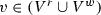, $k\in {\mathbb {R}}\cup \{\mathtt {undef}\}$ and $\odot \in \varSigma$; or

• (), where , and $\odot \in \varSigma$.

We denote by ${\mathcal {C}}_V$ the set of all possible simple guards on $V$.

A simple guard of the form (in this paper, k always denotes a constant) captures a condition requiring that the current value of the variable is compared with k through $\odot$. For instance, $(\mathtt {a}^r \ge \mathtt {0})$ expresses that the current value of $\mathtt {a}$ is greater or equal to $\mathtt {0}$. Similarly, the simple guard imposes a restriction on the new value of variable (that is being written by the transition to which this guard is associated). For example, $(\mathtt {a}^w > \mathtt {0})$ specifies that the new value of $\mathtt {a}$ is positive. Simple guards of the form and are analogous, but relate to the current value of a variable . If needed, we can express a simple guard that is always true by any tautological condition (such as . Parentheses around simple guards are only used for readability, and may be omitted.

In this paper we do not restrict ourselves to DPNs in which only the simple data conditions as above can be associated to transitions, but extend the model in [19] to also account for arbitrary boolean combinations of simple guards. Hence we consider the set $Guards _V$ defined as follows.

Definition 5

Given a set $V$ of variables and the set ${\mathcal {C}}_V$ of simple guards defined on $V$, we denote by $Guards _V$ the set of guards obtained by the grammar:

$$\begin{aligned} g \doteq sg ~|~ g_1 \wedge g_2 ~|~ g_1 \vee g_2 \end{aligned}$$

where $sg$ is a simple guard in ${\mathcal {C}}_V$.

As a result, a guard is either a simple guard or a boolean combination of simple guards. Note that, since the set $\varSigma$ of operators is closed under negation, the negation of a simple guard can always be expressed as another simple guard: it is sufficient to replace the predicate with its negation. For instance, the negation of $( \mathtt {a}{\;=\;} \mathtt {b})$ is $( \mathtt {a}\ne \mathtt {b})$. By extending this to arbitrary guards, we can in fact express the negation of any guard without the need of an explicit operator in the language of guards. Nonetheless, if needed, for convenience we write $\lnot g$ to denote the negation of a guard g.

We define a state variable assignment as a function $\alpha : V\mapsto {\mathbb {R}}\cup \{\mathtt {undef}\}$, used for specifying the current value of all variables.

Definition 6

A DPN ${\mathcal {N}} =\langle Pl,T,F,V,\alpha _I, guard \rangle$ is a Petri net $\langle Pl,T,F\rangle$ with additional components:

• $V$ is a finite set of process variables, as above;

• $\alpha _I$ is the initial state variable assignment, specifying the initial value of variables;

• $guard : T\mapsto Guards _V$ assigns a guard to each transition.

The variables in $V$ that are read and written by a guard g are, respectively, denoted by $read (g)$ and $write (g)$. For instance, $read ((\mathtt {a}^r {=} \mathtt {b}^r) \vee (\mathtt {a}^r {<} \mathtt {10})) {=} \{\mathtt {a},\mathtt {b}\}$, $read ((\mathtt {a}^w\ge \mathtt {\mathtt {b}^r}) {=} \{\mathtt {b}\}$, $write ((\mathtt {a}^r {<} \mathtt {3}) \wedge (\mathtt {b}^r {=} \mathtt {a}^r) )=\emptyset$. To ease the notation, given $t \in T$ we write as shorthand , and analogously $write ( t )$.

Moreover, we assume that a DPN is always associated with an arbitrary initial marking $M_I$ and an arbitrary final marking $M_F$. When $M_F$ is reached the execution of the process instance ends.

To define the execution of DPNs, we need a way to relate the state variable assignment s before and after a transition is fired. A guard variable assignment is a function $\beta : (V^r\cup V^w) \mapsto {\mathbb {R}}\cup \{\mathtt {undef}\}$, which assigns a value to read and written variables. As the name suggests, these assignments are used to specify the values of variables for evaluating the guards associated to transitions, as we intuitively described above. In general, this requires to compare previous and current values. The difference with a state variable assignment $\alpha$ is that $\beta$ is used for evaluating transition guards, while a state variable assignment holds the current value of each variable in $V$.

Given a guard variable assignment $\beta$ and a simple guard sg, we say that sg is satisfied by $\beta$ if and only if the guard is true after assigning values to variables as per $\beta$. Consider for example the simple guard : if then the guard is true if and only if the comparison $\odot (k',k)$ is true. For , this requires $\odot (k_1,k_2)$ with , . The case for is analogous.

We denote that a simple guard sg is true given a guard variable assignment $\beta$ by writing . For instance, a simple guard imposes that is updated with a value greater than its current value. For $\beta$ with $\beta (\mathtt {a}^w)=3$ and $\beta (\mathtt {a}^r)=2$, then .

As we discussed already, although we restrict here to variables of domain ${\mathbb {R}}$, our formalization is able to handle multiple domain types at once. Nonetheless, even with this restriction in place, we still need to deal with the case in which variables or values of distinct types are compared, as $\mathtt {undef}$ is not a real value. Therefore, we impose that only values with the same domain can be compared, otherwise the comparison is assumed to be always false, with the exception of ($\mathtt {undef}=\mathtt {undef}$). In other words, if an only if and $\odot$ is $=$.

We extend this to boolean combinations, hence to arbitrary guards, in the trivial manner, so that if and only if and , and similarly if and only if or .

Fig. 4

A simple DPN ${\mathcal {N}}$, with initial configuration $([p_0],\{\alpha _I(\mathtt {a})=\mathtt {0}, \alpha _I(\mathtt {b})=\mathtt {10}\})$

Example 5

Consider as an example the DPN in Fig. 4, in which two variables $\mathtt {a}$ and $\mathtt {b}$ exist with initial values $\mathtt {0}$ and $\mathtt {10}$, respectively (namely $\alpha _I(\mathtt {a})=\mathtt {0}$ and $\alpha _I(\mathtt {b})=\mathtt {10}$). From the initial marking $M_I=[p_0]$ a transition $t_1$ updates the value of $\mathtt {a}$ to any integer greater of $\mathtt {0}$ and not equal to $\mathtt {5}$. Then, either $t_2$ or $t_3$ are executable, depending on the current value assigned in $t_1$. Similarly, $t_4$ can be executed only if the current value of $\mathtt {b}$ (which is never updated) is smaller than the current value of $\mathtt {a}$. One can easily verify, by visual inspection, that the only possible sequence of transition that reaches the final marking is $t_1$, $t_2$, $t_4$, and that, obviously, not every value assigned to variable $\mathtt {a}$ allows to reach the end of the process. However, arbitrarily complex nets do not allow visual inspection to be carried out comprehensively, so that a simplistic analysis that disregards the possible state variable assignment s at each step, and thus only considers the control-flow of the net, could easily lead to wrong conclusions. In this case, from the fact that, apparently, all transitions and places are reachable in the control flow, we could naively conclude that there are no dead transitions and that it is always possible to reach the final marking avoiding deadlocks, i.e., that the net is classically sound.

We are finally ready to formalize the execution semantics of DPNs. The set of possible configuration s of ${\mathcal {N}}$ is the set of all pairs $(M,\alpha )$ where M is a marking of ${\mathcal {N}}$ and $\alpha$ is the (current) state variable assignment. From a configuration $(M,\alpha )$, a transition $t$ can be fired so to reach the new configuration $(M',\alpha ')$ only if $M[ t \rangle M'$⁴ and $\alpha '$ represents a possible update of $\alpha$ (defined next) which satisfies the guard $guard ( t )$, i.e., so that . A pair $( t ,\beta )$ where $t \in T$ and $\beta$ is a guard variable assignment is called transition firing.

Definition 7

A DPN ${\mathcal {N}} =\langle Pl,T,F,V,\alpha _I, guard \rangle$ evolves from configuration $(M,\alpha )$ to configuration $(M',\alpha ')$ by transition firing $( t ,\beta )$ iff $M[ t \rangle M'$ and:

• for every : the guard variable assignment $\beta$ assigns the same values as $\alpha$ to read variables;

• the new state variable assignment $\alpha '$ is as $\alpha$ but updated as per $\beta$ for the variables that are written. Namely, for all , we have if , otherwise ;

• : the guard is satisfied by $\beta$.

Essentially, a transition firing fully specifies a transition execution: it specifies the transition label and all the variable values before and after the transition is executed. For instance, referring again to Fig. 4, from the initial configuration, the transition firing $(t_1, \beta )$ with $\beta (\mathtt {a}^w)=\mathtt {7}$ results in the new configuration $([p_1],\{\alpha '(\mathtt {a})=\mathtt {7}, \alpha '(\mathtt {b})=\mathtt {0}\})$.

We denote a transition firing $( t ,\beta )$ as in Definition 7, from configuration $(M,\alpha )$ to configuration $(M',\alpha ')$, by writing . We also extend this definition to sequences of the form $\sigma = (t_1,\beta _1)\cdots (t_n,\beta _n)$ and thus define runs as the sequences of the form , also denoted as . Moreover, we write to mean that there exists a non-empty sequence $\sigma$ as above that reaches $(M_n,\alpha _n)$.

A run of ${\mathcal {N}}$ is a run as above starting from $(M_I,\alpha _I)$, that is, from the configuration obtained by considering the initial marking and the initial state variable assignment. We denote by $Reach_{{\mathcal {N}}}$ the set of configuration s that are reachable by a run of ${\mathcal {N}}$, namely .

Finally, given two markings $M'$ and M of a DPN ${\mathcal {N}}$, we write $M' \ge M$ (and say that $M'$ is larger than or equal to M) iff for each place $p \in Pl$ in ${\mathcal {N}}$ we have $M'(p) \ge M(p)$, and we write $M' > M$ iff $M' \ge M$ and there exists $p \in Pl$ s.t. $M'(p) > M(p)$. When needed, we write $M' \not \ge M$ to indicate that it is not the case that $M' \ge M$. A configuration $(M,\alpha )$ so that $M\ge M_F$ is called final, since the process has reached the final marking on the underlying Petri net.

4.2 Encoding DBPMN into DPNs

We now show how a DBPMN process ${\mathcal {B}}$ can be encoded into a corresponding DPN, in turn defining the execution semantics of ${\mathcal {B}}$. The translation works in three steps.

The DPN resulting from the application of the three steps detailed in this section on the DBPMN in Fig. 1 is shown in Fig. 5.

Fig. 5

DPN encoding of the DBPMN model in Fig. 1 (once having collapsed the three end-events of the process into a single one), using the control-flow encoding of BPMN into Petri nets from [24]. The initial and final markings $M_I$ and $M_F$ have a single token in the first/last place, respectively. For space reasons, we use compact names for the variables corresponding to the data objects of the DBPMN model. Internal transitions used to capture events and gateways are shown in gray, whereas transitions mirroring actual tasks are shown in white, and associated to a meaningful label. Guards are shown in disjunctive normal form and semantically simplified, and we use therein atoms of the form $x \in ( k_1,k_2 ]$ as a shorthand for $(x > k_1) \wedge (x \le k_2)$, and $x \not \in (k_1,k_2 ]$ as a shorthand notation for $(x \le k_1) \vee (x > k_2)$. Dead transitions, which can never be executed starting from the initial configuration that assigns one token to the topmost place and assumes that all data objects are initially undefined, are shown in red (cf. Example 11)

Step 1: control-flow. The first step consists in the encoding of the control-flow of the BPMN process ${\mathcal {B}}. P$ into a corresponding Petri net, by ignoring case data and decisions. This can be achieving by an off-the-shelf use of any of the encoding procedures available in the literature, such as the one by Dijkman et al. fig[24]. To give an intuition on how the control-flow of the BPMN process can be encoded into a Petri net by following the cited approach, we report in [24] a depiction of how the basic BPMN elements are encoded, taken directly from Fig 6. This encoding is adopted in Fig. 5 to formally represent the BPMN constructs employed in Fig. 1. The reader can refer to that work for details on how further BPMN elements and subprocesses can be encoded as well.

Two observations are in place when it comes to the BPMN control-flow and its Petri net encoding in our setting. First, it is important to stress that the elements shown in Fig 6 and more in general the encoding introduced in [24], only cover the core BPMN constructs; representing more advanced constructs such as or joins and interrupting boundary events calls for more sophisticated formal models, such as Petri nets with cancellation regions and equipped with other advanced constructs (see, e.g., [25] and the Petri net-based encoding of advanced workflow patterns⁵). Second, as it will become apparent in Sect. 5, our formal analysis for DBPMN is based on the combination of standard control-flow analysis techniques for Petri nets and faithful data abstraction techniques for tackling the data dimension. This combination continues to hold even when the control-flow part employs the more advanced constructs mentioned above. The main issue, in this setting, is that even in the pure control-flow case all basic properties becomes undecidable, unless one ensures that the net is bounded (in the standard Petri net sense). This is actually a standard assumption in soundness analysis, where a single case is expected to generate only boundedly many concurrent threads of control.

Fig. 6

Figure taken from [24], depicting how task, events, and gateways can be encoded as Petri nets

From now on, we then assume to have a black-box, control-flow encoding function $encodeFlow$ that, given a BPMN model ${\mathcal {B}}. P$, transforms it into a Petri net $encodeFlow ({\mathcal {B}}. P )$ that captures the control-flow execution semantics of ${\mathcal {B}}. P$, with the following assumptions⁶:

• every business rule task $t\in {\mathcal {B}}. P .\mathsf {brTasks}$ becomes a distinct transition $t$ in the Petri net $encodeFlow ({\mathcal {B}}. P )$, with a single input place (representing the enablement of the task) and a single output place (representing the completion of the task). Note that this restriction is assumed only on (business rule) tasks and not, for instance, on the encoding of choice gateways, joins, etc. This assumption is thus made without loss of generality. Moreover, note that the encoding in [24] is consistent with this assumption (see Fig 6). Whenever needed, we denote the input and output places for a given $t$ as $p_i^t$ and $p_o^t$, respectively;

• for every choice gateway $gway\in {\mathcal {B}}. P .\mathsf {choicePoints}$, each conditional flow $s\in gway.\mathsf {condFlows}$ (that is, each sequence flow departing from $gway$) is mapped to a distinct transition $s$ in $encodeFlow ({\mathcal {B}}. P )$. Also this requirement is met by the encoding in [24] (see bottom-left of Fig 6).

It is easy to show that such a black-box encoding does not alter the structure of the original process, so that the resulting DPN can be analyzed to assess correctness. Accordingly, with a slight abuse of notation, in this paper we use the same symbol to denote a BPMN task or sequence flow and its corresponding DPN transition, since these are in direct correspondence.

Step 2: expansion of business rule tasks. Since business rule tasks are linked to DMN tables, we have to enhance the Petri net $encodeFlow ({\mathcal {B}}. P )$ obtained in the first step so as to explicitly account for the firing of table rules. This is done as follows. Given a business rule task $t\in {\mathcal {B}}. P$.$\mathsf {brTasks}$, we denote by $DecRows_{{\mathcal {B}}}(t)$ the set of additional transitions that represent all possible modes of applying the decision table $d = {\mathcal {B}}.\mathsf {taskToDec}(t)$ attached to $t$. These correspond to the rules $d.{R}$ in the decision table d (indexed by their position), together with an additional transition with special index $\mathsf {noRow}$. The latter accounts for the case where no rule in d matches the given inputs (and, consequently, the default outputs, or alternatively $\mathtt {undef}$ values, have to be produced in output). Specifically:

$$\begin{aligned} DecRows_{{\mathcal {B}}}(t) \doteq \{ t^j \mid j \in \{1,\ldots ,|d.{R}|\}\} \cup \{ t^\mathsf {noRow}\} \end{aligned}$$

According to $encodeFlow ({\mathcal {B}}. P )$ (see Step 1), each business rule task $t\in {\mathcal {B}}. P .\mathsf {brTasks}$ is translated into a transition having one input place $p_i^t$ and one output place $p_o^t$. In the expansion of $encodeFlow ({\mathcal {B}}. P )$, which we also denote by $encodeFlow ({\mathcal {B}})$ each transition $t\in {\mathcal {B}}. P$.$\mathsf {brTasks}$ as above is replaced by the set $DecRows_{{\mathcal {B}}}(t)$ of transitions, so that each of such transitions has $p_i^t$ as single input place and $p_o^t$ as single output place. This captures that whenever a token is present in $p_i^t$, then one rule of the table ${\mathcal {B}}.\mathsf {taskToDec}(t)$ can nondeterministically fire, marking the completion of the task by producing a token in $p_o^t$ (recall that ${\mathcal {B}}.\mathsf {taskToDec}(t)$ is a unique-hit table—cf. the end of Sect. 3.2). The guards attached to these transitions will be discussed in Step 3.

All in all, we denote by $Tasks({\mathcal {B}})$ all the transitions that correspond to tasks in ${\mathcal {B}}$, that is, manual tasks or rule-indexed business rule tasks:

$$\begin{aligned} Tasks({\mathcal {B}}) \doteq {\mathcal {B}}. P .\mathsf {manTasks} \cup \bigcup _{t\in {\mathcal {B}}. P .\mathsf {brTasks}} DecRows_{{\mathcal {B}}}(t) \end{aligned}$$

Example 6

Figure 5 shows the full DPN encoding of the DBPMN diagram in Fig. 1. The initial part of the net encodes the message reception event, the $\mathsf {measure~weight}$ and the $\mathsf {get~length}$ tasks. The latter explicitly shows the expansion discussed so far: in place of having a single transition, we have four alternative transitions $\mathsf {get~length}^j$, $j\in \{1,2,3,\mathsf {noRow}\}$, denoting the application of one of the three rules in the corresponding DMN table plus one for the situation where no rule matches. The computation of the guards associated to these transitions is part of the next step.

Step 3: variables and guards. The third step requires to transform the guards and decision rules present in ${\mathcal {B}}$ into DPN guards conforming to Definition 5. Two aspects have to be considered here: (i) S-FEEL conditions (as in Definition 1) and their combination into rules have to be suitably encoded into proper boolean formulae; (ii) suitable read/write variables have to be employed when building such formulae.

In the following, we directly employ column names and data objects as variables. In addition, we denote by $Vars (\varphi )$ the set of (data object) variables appearing in the boolean formula $\varphi$. We also make use of the standard notion of variable substitution to replace, in boolean formulae, a variable denoting a data object or table column with a corresponding read/written DPN variable. Given a boolean formula $\varphi$ and a variable substitution function $\theta$ defined over $Vars (\varphi )$, we write $\varphi _{[\theta ]}$ to denote the boolean formula obtained from $\varphi$ by replacing each data object $\mathbf {a}$ with $\theta (\mathbf {a})\in V$. Note that, however, $\varphi _{[\theta ]}$ is still not a guard as in Definition 5, because it is defined on variables in $V$ rather than on $(V^r\cup V^w)$. This is done next, for the various cases.

The first and most direct case is that of conditional flows in ${\mathcal {B}}$, namely sequence flows with attached conditions. These conditions are in fact already boolean formulae, so it is enough to make sure that all the involved variables appear as read variables (i.e., in $V^r$), witnessing that they are used to evaluate the condition. Given a condition $\varphi \in {\mathcal {B}}. P .\mathsf {choiceGuard}(gway)$ for some choice gateway $gway\in {\mathcal {B}}. P .\mathsf {choicePoints}$, we denote by $encode Test (\varphi )$ the DPN guard (in the sense of Definition 5) obtained from $\varphi$ by substituting each variable by its corresponding read version .

Example 7

Consider the first choice gateway in Fig. 1. The encoding of the guards attached to the two conditional branches correspond to guards $(\mathsf {pLength}^r = \mathtt {undef}) \vee (\mathsf {pWeight}^r > 10)$ and $(\mathsf {pLength}^r \ne \mathtt {undef}) \wedge (\mathsf {pWeight}^r \le 10)$.

The encoding of write guards and decision tables is more involved, as this requires to perform additional manipulations. As a basic building block, we need to define how to encode an S-FEEL condition (as of Definition 1) into a corresponding DPN guard. To this end, we build on prior work on the logical formalization of DMN [7]. Specifically, given an S-FEEL condition $\varphi$ with external parameters X and variable , we define the DPN guard for $\varphi$ relatively to v, as follows:

We can directly use this encoding to define the DPN guard corresponding to the update induced by the execution of a manual task $t\in {\mathcal {B}}. P .\mathsf {manTasks}$, by encoding its output data objects and their associated condition (business rule tasks are encoded differently, on the basis of their associated decision tables). When no condition is specified for some output data object, then we assume an implicit condition $\varphi = ``-\hbox {''}$. This DPN guard, denoted by $encode Update _{\mathcal {B}}(t)$, simply amounts to the conjunction of the encoding of each write guard, considering as variables the write variables corresponding to the output data objects of the manual task $t$:

$$\begin{aligned}&encode Update _{\mathcal {B}}(t) \doteq \bigwedge _{o \in {\mathcal {B}}.\mathsf {outObj}(t)}\\&encodeSFEEL ^{o^w}\Big ({\mathcal {B}}.\mathsf {writeGuard}\big (\langle t,o\rangle \big )\Big ) \end{aligned}$$

Example 8

Consider the manual task $\mathsf {measure~weight}$ in Fig. 1. It has a single output data object, namely $\mathsf {pWeight}$, and the write guard associated to this output is the S-FEEL condition $``{>}0''$. We then have:

$$\begin{aligned} encode Update (\mathsf {measure~weight}) = (\mathsf {pWeight}^w>0) \end{aligned}$$

Intuitively, a similar encoding is used for determining the guards associated to DPN transitions corresponding to rules of decision tables, such as those mentioned in Example 6. Recall that each such rule encodes an input–output relation between the input and output attributes of the table, dictating that every input attribute must be conforming to its facet and must also satisfy the corresponding S-FEEL condition, whereas every output attribute must match with the corresponding value/parameter. Once this conjunctive formula is built, we then replace the input/output attributes and parameters used therein with the data objects that are mapped to them, by considering that while input conditions read the corresponding variables and parameters, output conditions write them. After this encoding is completed, we then add an additional, ad-hoc formula to capture the case where no rule applies (i.e. the $\mathsf {noRow}$ transition commented in Example 6), and consequently the result produced for each output attribute corresponds to its default value (if defined), or to $\mathtt {undef}$ (if no default value is specified in the table).

The intuitive encoding just described in formalized as follows. Consider a business rule task $t\in {\mathcal {B}}. P .\mathsf {brTasks}$, and let $\theta = {\mathcal {B}}.\mathsf {objToDec}(t)$ be the table-to-object map associated to $t$. Since we use column names and data objects as variables in the DPN, then $\theta$ can be used as a variable substitution function. The encoding of the premise of rule $\langle \mathsf {If},\mathsf {Then}\rangle \in {\mathcal {B}}.\mathsf {taskToDec}(t).{R}$ is defined as $encodeIf _{{\mathcal {B}},t}(\langle \mathsf {If},\mathsf {Then}\rangle ) \doteq$

The core part of the formalization above is the boolean formula testing that $\mathbf {a}$ satisfies the condition assigned to $\mathbf {a}$ by the rule; this is obtained by encoding the S-FEEL condition $\mathsf {If}(\mathbf {a})$ through the $encodeSFEEL$ procedure. The so-obtained formula, denoted by $\varphi$ in what follows, requires, for the rule to match, that all input conditions satisfy the three criteria above. However, $\varphi$ is not yet a DPN guard as in Definition 5. First, since $\mathbf {a}$ is mapped through $\theta$ to a corresponding data object of ${\mathcal {B}}$, we need to replace $\mathbf {a}$, as well as the parameters possibly mentioned in the input conditions, to corresponding data objects as dictated by $\theta$. Second, we need to apply the $encode Test$ function to $\varphi$. This function simply replaces all the data object variables in $Vars (\varphi )$ to their corresponding read version in $V^r$. The so-obtained formula is a guard as in Definition 5, capturing the required test on (read) variables.

Next, the encoding of the result of applying a rule $\langle \mathsf {If},\mathsf {Then}\rangle$ is defined as the guard $encodeThen _{{\mathcal {B}},t}(\langle \mathsf {If},\mathsf {Then}\rangle ) \doteq$

This encoding handles the update of output attributes (i.e., output attributes of the decision table ${\mathcal {B}}.\mathsf {taskToDec}(t)$) with the output values/parameters mentioned by the rule. As in the case of the rule premise, we have to take care of the fact that each output attribute $\mathbf {b}$ needs to be substituted with the corresponding data object as per $\theta$ (which is then used as DPN variable). Therefore, since the output attributes are produced as output, we encode this through a variable that is written (hence in $V^w$). Moreover, note that we separately consider the case where the output is an actual value (which is simply assigned to the variable), and the case where the output is a parameter (which needs to be replaced by the reading of the data object assigned to the parameter by $\theta$). If multiple output attributes are present, their corresponding formulae need to be conjoined together.

To obtain the full encoding of the rule as a DPN guard, the two encodings of the premise and consequence parts of the rule have to be accompanied by a further part, which checks the “well-formedness” of the involved attributes by verifying, for each input attribute $\mathbf {a}$:

• 1. that $\mathbf {a}$ is not $\mathtt {undef}$. This check is needed because, as explained in Sect. 4.1, simple guards can be true only if the compared variables and values are of the same type (recall that $\mathtt {undef}\not \in {\mathbb {R}}$);

• 2. that $\mathbf {a}$ satisfies its facet condition. This is obtained by encoding the S-FEEL condition $\mathsf {InFacet}(\mathbf {a})$ through the $encodeSFEEL ^{\mathbf {a}}$ procedure.

Formally, the resulting formula for well-formedness, defined by using the same approach as that of $encodeIf _{{\mathcal {B}},t}$, is $encodeWF _{{\mathcal {B}},t} \doteq$

As a result, the input–output relation induced by the entire rule $\langle \mathsf {If},\mathsf {Then}\rangle$ is then captured by the DPN input–output guard $encodeRule _{{\mathcal {B}},t}(\langle \mathsf {If},\mathsf {Then}\rangle ) \doteq$

$$\begin{aligned}&encodeWF _{{\mathcal {B}},t} \wedge encodeIf _{{\mathcal {B}},t}(\langle \mathsf {If},\mathsf {Then}\rangle ) \wedge encodeThen _{{\mathcal {B}},t}(\langle \mathsf {If},\mathsf {Then}\rangle ) \\&{}\wedge \bigwedge _{\mathbf {b} \in {\mathcal {B}}.\mathsf {taskToDec}(t).O} encodeSFEEL ^{\theta (\mathbf {b})^w}\big (\mathsf {InFacet}(\mathbf {b})\big ) \end{aligned}$$

where we also include an additional well-formedness test for the produced output, so as to ensure that the written value of each output attribute is matched by the corresponding facet condition. This conjunct is redundant when the table contains explicit output values (provided that these have the right type, namely are in the facet).

Example 9

We discuss how the first rule of the decision table attached to the $\mathsf {determined~mode}$ task in Fig. 1 is encoded into a DPN guard. The S-FEEL condition associated to the $\mathbf {Length}$ attribute is encoded through $encodeSFEEL ^{\mathbf {a}}$ (that is, $encodeSFEEL ^{\mathbf {Length}}$) into $(\mathbf {Length} > 0) \wedge (\mathbf {Length} \le 1)$, whereas the S-FEEL condition associated to the $\mathbf {Weight}$ attribute is encoded as $(\mathbf {Weight}>0) \wedge (\mathbf {Weight} \le 5)$. The resulting conjunctive formula is subject to the application of the table-to-object map associated to the $\mathsf {determined~mode}$ task, which maps attribute $\mathbf {Length}$ to data object $\mathsf {pLength}$, and $\mathbf {Weight}$ to $\mathsf {pWeight}$. $\mathsf {pLength}$ and $\mathsf {pWeight}$ are thus used as DPN variables. The application of $encode Test$ then ensures that $\mathsf {pLength}$ and $\mathsf {pWeight}$ are read, thus producing, for the input part of the rule, the formula $(\mathsf {pLength}^r>0) \wedge (\mathsf {pLength}^r\le 1) \wedge (\mathsf {pWeight}^r>0) \wedge (\mathsf {pWeight}^r\le 5)$. Similarly, the output attribute $\mathbf {mode}$ is assigned by the rule to the value $\mathtt {car}$, and is substituted with data object $\mathsf {sMode}$ by the table-to-object map associated to the $\mathsf {determined~mode}$ task. So, its encoding produces formula ($\mathsf {sMode}^w = \mathtt {car}$). Considering the contribution of the attribute facets, and the additional tests ensuring that the attributes are defined, the encoding of the rule produces, overall:

$$\begin{aligned}&(\mathsf {pLength}^r \ne \mathtt {undef}) \wedge (\mathsf {pWeight}^r \ne \mathtt {undef}) \wedge (\mathsf {pLength}^r>0) \\ {}\wedge {}&(\mathsf {pWeight}^r>0) \wedge (\mathsf {pLength}^r>0) \\&\quad \wedge (\mathsf {pLength}^r\le 1) \wedge (\mathsf {pWeight}^r>0) \\ {}\wedge {}&(\mathsf {pWeight}^r\le 5) \wedge (\mathsf {sMode}^w = \mathtt {car}) \end{aligned}$$

which can be simplified into the logically equivalent, simpler formula:

$$\begin{aligned}&(\mathsf {pLength}^r>0) \wedge (\mathsf {pLength}^r\le 1) \wedge (\mathsf {pWeight}^r>0) \\&\quad \wedge (\mathsf {pWeight}^r\le 5){}\wedge {}(\mathsf {sMode}^w = \mathtt {car}) \end{aligned}$$

The formula induces an input–output relation established by task $\mathsf {determined~mode}$ between the two input data objects $\mathsf {pLength}$ and $\mathsf {pWeight}$ and the output data object $\mathsf {sMode}$.

Finally, we have to handle the default situation where no rule of a table matches, by writing the guard to be associated to the $t^{\mathsf {noRow}}$ DPN transition, for each business rule task t. We distinguish, in this respect, two reasons for this:

• 1. no rule matches because the provided input is not well-formed, that is, it contains undefined values or values that do not respect the facet conditions of their associated table attributes. In this case, we output $\mathtt {undef}$ for all the output attributes, witnessing the inapplicability of the decision logic;

• 2. no rule matches because, even though the provided input is well-formed, it violates at least one input condition in each of the rules in the table. In this case, for every output attribute we produce as a result the default value assigned to the attribute, or $\mathtt {undef}$ if no such a default value is given.

Considering again a business rule task $t$ and $\theta$ as above, this is defined as the DPN formula $encodeDefaultRule _{\mathcal {B}}(t) \doteq$

where $\mathsf {ODef}$ is the function assigning a default value for the decision table ${\mathcal {B}}.\mathsf {taskToDec}(t)$, as in Definition 2. The first disjunct captures the case where the table cannot be applied due to non-well-formedness (case 1), so $\mathtt {undef}$ values are written in output. The second disjunct instead handles the case where well-formedness is satisfied (case 2). For this case, the resulting guard is divided in two parts (corresponding to the two lines in the formula above, in the second disjunct). The first line requires that the default formula is applied when none of the rule premises holds (i.e., $\lnot encodeIf _{{\mathcal {B}},t}(r)$ for each rule r). The second line specifies which output value is written into each data object (hence variable) to which the output attribute is mapped by $\theta$: either the default value (if present) or the $\mathtt {undef}$ value.

Example 10

Consider again the $\mathsf {determined~mode}$ task in Fig. 1. The default formula associated to this task captures the situation where the execution of the task, that is, the application of its associated decision table, results in an undefined shipment mode (note that no default output value is defined). This is formalized as a guard indicating that $\mathsf {sMode}$ is undefined whenever the involved attributes are either undefined, do not respect their facet conditions, or they do but none of the rules applies:

$$\begin{aligned} \begin{array}{@{}l@{}l@{}} &{} \left( \begin{array}{@{}l@{}} \left( \begin{array}{@{}l@{}l@{}} &{} \mathsf {pLength}^r = \mathtt {undef}\\ {}\vee &{} \mathsf {pWeight}^r = \mathtt {undef}\\ {}\vee &{} \mathsf {pLength}^r \le 0\\ {}\vee &{} \mathsf {pWeight}^r \le 0\\ \end{array} \right) \wedge (\mathsf {sMode}^w = \mathtt {undef}) \end{array} \right) \\ \vee &{} \left( \begin{array}{@{}l@{}} \left( \begin{array}{@{}l@{}l@{}} &{} \mathsf {pLength}^r \ne \mathtt {undef}\wedge \mathsf {pWeight}^r \ne \mathtt {undef}\\ \wedge &{} \mathsf {pLength}^r> 0 \wedge \mathsf {pWeight}^r> 0\\ \wedge &{} \left( \begin{array}{@{}l@{}l@{}} &{} (\mathsf {pWeight}^r> 10)\\ {}\vee &{} \left( \begin{array}{@{}l@{}} \mathsf {pWeight}^r \le 5 \wedge \mathsf {pLength}^r > 2\\ \end{array} \right) \end{array} \right) \end{array} \right) \wedge (\mathsf {sMode}^w=\mathtt {undef}) \end{array} \right) \end{array} \end{aligned}$$

This can be semantically simplified into:

$$\begin{aligned} \begin{array}{@{}l@{}l@{}} &{} \left( \begin{array}{@{}l@{}} \left( \begin{array}{@{}l@{}l@{}} &{} \mathsf {pLength}^r = \mathtt {undef}\\ {}\vee &{} \mathsf {pWeight}^r = \mathtt {undef}\\ {}\vee &{} \mathsf {pLength}^r \le 0\\ {}\vee &{} \mathsf {pWeight}^r \le 0\\ \end{array} \right) {}\wedge (\mathsf {sMode}^w = \mathtt {undef}) \end{array} \right) \\ \vee &{} \left( \begin{array}{@{}l@{}} \begin{array}{@{}l@{}l@{}} \left( \begin{array}{@{}l@{}l@{}} &{} (\mathsf {pWeight}^r> 10)\\ {}\vee &{} \left( \begin{array}{@{}l@{}} \mathsf {pWeight}^r> 0 \wedge \mathsf {pWeight}^r \le 5 \wedge \mathsf {pLength}^r > 2\\ \end{array} \right) \end{array} \right) \end{array} \wedge (\mathsf {sMode}^w=\mathtt {undef}) \end{array} \right) \end{array} \end{aligned}$$

Putting everything together We are now ready to define the overall encoding of ${\mathcal {B}}$ into a corresponding DPN. The DPN of ${\mathcal {B}}$ is the net $\text {DPN}({\mathcal {B}}) \doteq \langle Pl,T,F,V,\alpha _I, guard \rangle$, where:

• the net backbone consists of the expansion of the Petri net encoding of ${\mathcal {B}}. P$, that is, $\langle Pl,T,F\rangle = encodeFlow ({\mathcal {B}})$;

• the net variables are the data objects of ${\mathcal {B}}$, that is, $V= {\mathcal {B}}. P .\mathsf {dataObj}$;

• $\alpha _I$ is so that every data object is initialized to the $\mathtt {undef}$ value;

• $guard$ associates to each conditional flow transition its corresponding DPN test guard, to each manual task its corresponding DPN update guard, and to each decision rule transition its corresponding DPN rule input–output guard. Formally, $guard$ is defined as:

  • for every choice gateway $gway\in {\mathcal {B}}. P .\mathsf {choicePoints}$ and every conditional flow transition $t\in {\mathcal {B}}. P .\mathsf {condFlows}(gway)$, we have $guard (t) = encode Test ({\mathcal {B}}.\mathsf {choiceGuard})$;

  • for every manual task $t\in {\mathcal {B}}. P .\mathsf {manTasks}$, we have $guard (t) = encode Update _{{\mathcal {B}}}(t)$;

  • for every business rule task $t\in {\mathcal {B}}. P .\mathsf {brTasks}$ and every rule $r_i \in {\mathcal {B}}.\mathsf {taskToDec}(t).{R}$ with position i in the associated table, we have $guard (\langle t,i\rangle ) = encodeRule _{{\mathcal {B}},t}(r_i)$;

  • for every business rule task $t\in {\mathcal {B}}. P .\mathsf {brTasks}$, we have $guard (\langle t,\mathsf {noRow}\rangle ) = encodeDefaultRule _{{\mathcal {B}}}(t)$;

  • for every other transition $t\in T$, $guard (t)$ is assumed to a tautological guard.

5 Soundness Analysis of DBPMN Processes

In this section we consider a set of properties that can be used to characterize various notion of correctness of a process in terms of soundness. These properties include (an adaptation of) those introduced in [11], which are combined in that work to define various notions of decision-aware soundness. First, in Sect. 5.1 we formalize these properties directly on DPNs, as we have captured the execution semantics for DBPMN through these nets. Then, in Sect. 5.2, we detail how these properties can be verified by relying on a known verification technique for DPNs.

5.1 Notions of Data-Aware Soundness of DBPMN Processes

Given a DBPMN process ${\mathcal {B}}= \langle P ,\mathsf {writeGuard},\mathsf {choiceGuard},D,\mathsf {taskToDec},\mathsf {objToDec}\rangle$, let $\text {DPN}({\mathcal {B}}) =\langle Pl,T,F,V,\alpha _I, guard \rangle$ be the DPN defined in the previous section. We define the following properties on $\text {DPN}({\mathcal {B}})$, adopting when possible the names and terminology of [11]:

• P1 (Option to Complete) For each reachable configuration that is not final there is always an option to reach a final configuration. Formally, $\forall (M, \alpha )\in Reach_{\text {DPN}({\mathcal {B}})}$. $M \not \ge M_F$ $\Rightarrow$ $\exists \alpha '$. .⁷

• P2 (Clean completion) Whenever a final configuration is reached, no token is left in the rest of the net and no task can still be executed. Formally, $\forall (M, \alpha )\in Reach_{\text {DPN}({\mathcal {B}})}$.  $M\ge M_F$ $\Rightarrow$ ($M=M_F$) $\wedge \not \exists t.~ M[t\rangle$.

• P3 (No dead task) For each transition t (corresponding to a manual task of ${\mathcal {B}}$, that is excluding transitions that encode rules of decision tables), there is at least one run that enables t. Formally, $\forall t\in {\mathcal {B}}. P .\mathsf {manTasks}$. $\exists M_1, M_2, \alpha _1,\alpha _2,\beta$. .

• P4 (DMN Conditional Completeness) Each DMN table always produces a result. This can be checked by requiring that, whenever it is enabled according to the control flow, a DPN transition $t^i$ that encodes a rule of a decision table for some business rule task $t\in {\mathcal {B}}. P$.$\mathsf {brTasks}$ (i.e., $t^i \in DecRows_{{\mathcal {B}}}(t)$), then at least one DPN transition $t^j$ encoding a rule of the same decision table can be fired (possibly with $i{=}j$). Moreover, if $j=\mathsf {noRow}$ then we require that a default output value exists, i.e., a default output value is given in output for the variable such that (with a little abuse of notation, we denote the new value of as $\alpha '( write (t^j))$). Formally, $\forall (M,\alpha )\in Reach_{\text {DPN}({\mathcal {B}})}$, $t\in {\mathcal {B}}. P$.$\mathsf {brTasks}$, $t^i \in DecRows_{{\mathcal {B}}}(t)$. $M[t^i \rangle \Rightarrow \exists t^j \in DecRows_{{\mathcal {B}}}(t), \beta , \alpha '.$ .

• P5 (DMN Conditional Output Coverage) No rule in DMN tables can cause a deadlock when hit. This can be modeled by requiring that, whenever a DPN transition $t^i$ that encodes a rule of the decision table associated to some $t\in {\mathcal {B}}. P$.$\mathsf {brTasks}$ is fired (including $i = \mathsf {noRow}$), then the execution can continue. Formally, $\forall (M,\alpha )\in Reach_{\text {DPN}({\mathcal {B}})}$, $t\in {\mathcal {B}}. P$.$\mathsf {brTasks}$, $t^i \in DecRows_{{\mathcal {B}}}(t), \beta ,\alpha '$. .

Fig. 7

The various notions of data-aware soundness, inspired to those of decision-aware soundness illustrated in [11]. The figure also shows to which properties these correspond in terms of the DBPMN behavioral properties. Note that $P1{-}P3$ correspond to the properties considered in [19] for arbitrary DPNs, with the difference that P3 is here adapted to DBPMN processes that distinguish manual and business rule tasks

For instance, in the DPN in Fig. 5, P4 requires that, whenever a transition $\mathsf {determine~mode}^i$ is enabled for some $i\in \{1,2,3,\mathsf {noRow}\}$, then at least one transition $\mathsf {determine~mode}^j$ can eventually fire, for some $j\in \{1,2,3,\mathsf {noRow}\}$. The same is required for all other business rule tasks.

By combining the five above properties, it is possible to express, on the DBPMN process ${\mathcal {B}}$ captured by $\text {DPN}({\mathcal {B}})$, various notions of soundness introduced in the literature. As already said, in what follow we consider possible adaptations of the different definitions of decision-aware soundness discussed in [11]. These properties are depicted in Fig. 7, where P1b and P1c are weaker versions of property P1, and P2b is a weaker version of property P2, defined below. The arc between two soundness notations indicate whether the source implies the target.

P1b::

It is possible to extend any run to reach a marking larger than or equal to the final marking if this did not happen already along the run: .

P1c::

A configuration with a marking larger than or equal to the final marking is reachable by at least one run: $\exists \alpha , M. ~(M,\alpha ) \in Reach_{\text {DPN}({\mathcal {B}})} \wedge M \ge M_F$.

P2b::

From any configuration with a marking larger than or equal to $M_F$ it is still possible to continue the execution, but is no more possible to again reach one such configuration: .

By adopting again the names of the decision-aware properties in [11], we define here various properties of data-aware soundness. The strongest property is that of Data-aware soundness, which is captured by requiring all properties P1–P5. A DBPMN process ${\mathcal {B}}$ for which P3 is true but P1 and P2 do not hold on $\text {DPN}({\mathcal {B}})$ is instead called Data-aware relaxed sound. In such processes, every manual task can participate in at least one process execution (P3), every DMN table is complete (P4) and none of its output leads to a deadlock (P5). A considerably weaker soundness notion is that of Data-aware easy soundness, where the only property is P1b: there is at least one process execution from the initial state to one of the final states. If instead only property P3 does not hold for $\text {DPN}({\mathcal {B}})$, then the DBPMN process ${\mathcal {B}}$ is said to be Data-aware weak sound. This means that there is always an option to complete, and in a clean manner, but some tasks might be dead (however, from P4 it follows that no decision task can be dead). Finally, a further weaker property is called Data-Aware Lazy Soundness, as it allows the DBPMN process to be lazy: the execution may continue after reaching a final state, hence violating P2, but it cannot again reach a new final state (P2b), and there is always an option to complete before reaching a final state for the first time (P1b).

For completeness, we also consider the following property, which corresponds to the counterpart of P3 for DPN transitions corresponding to rules in decision tables associated to business rule tasks.

• P6 (No dead table row): There is an execution that hits each row of each DMN table. This can be modeled by requiring that, for each transition t representing a row of a DMN table (but excluding the additional default rule that was added by the encoding), there exists a run that enables $t$. Formally, $\forall t\in {\mathcal {B}}. P$.$\mathsf {brTasks}$, $t^i \in DecRows_{{\mathcal {B}}}(t)$, $i\ne \mathsf {noRow}$. $\exists M_1, M_2, \alpha _1,\alpha _2,\beta$. .

Example 11

Given the DPN ${\mathcal {N}}$ shown in Fig. 5, assessing the properties discussed in this section is not a trivial task. It requires one to adopt the approach illustrated in Sect. 5.2, based on the verification technique in [19], to exhaustively account for any possible execution of the process. We simply comment here on the truth values of these formulae, assuming to have completed the verification procedure.

Properties P1 is true, although this is not evident by inspecting the DPN: from any reachable configuration of , it is always possible to reach the final marking. Intuitively, this means that the combination of the conditions associated to manual tasks and business rule tasks cannot induce neither a deadlock nor a livelock. As a consequence, P5 is true as well (it can be easily shown that P1 implies P5). Property P2 is also true, and this is evident by visual inspection: only one token exists in each reachable marking, so when a final configuration is reached, the termination is “clean”. Property P3 is instead false, although this is not evident by visual inspection: there are in fact dead transitions (marked in red in Fig. 5) and, between these, two encode manual tasks ($\mathsf {fetch~declaration}$ and the transition with guard $\left( \mathsf {sM}^r = \mathtt {undef}\right)$). This means that it is in fact not possible to assign $\mathtt {owner}$ as value of object $\mathsf {consent}$ and it is also never the case that the output of table Choose Consent is undefined (that is, that either the facet conditions are not satisfied or that no rule matches but there is no default value for this table – see the guard associated to transitions $\mathsf {choose~consent}^{\mathsf {noRow}}$). It can be verified that P4 is true for ${\mathcal {N}}$, since there are no runs of this process for which, at some point, a decision table cannot produce any result in output. Property P6 is violated: among the dead transitions marked in red in Fig. 5, one encodes a rule in a DMN table, namely $\mathsf {choose~consent}^{1}$: it can be shown that the first rule of $\mathsf {choose~consent}$ can never be matched.

All these issues were already commented on the original DBPMN process in Sect. 2, where the running example is introduced, although we are now able to employ automated verification techniques to detect such issues. Finally, note that two more transition are marked as dead in the figure, namely the two transitions immediately preceding and following the transition $\mathsf {fetch~declaration}$. However, these two transitions were added during the encoding for technical reasons and do not encode manual tasks nor rules of DMN tables, hence have no impact on the truth values of the properties we are considering (specifically, P3).

5.2 Verifying Notions of Data-Aware Soundness of DBPMN Processes

In previous work [19], we have shown how to check data-aware soundness of DPNs (as in the previous section) in spite of the fact that the possible runs of a DPN are in fact infinite in general, both in number and in length. The technique was then extended to account for arbitrary temporal formulae expressing requirements on both the control-flow and data [21]. The approach is based on an interval-abstraction technique that allows to represent all possible runs of a given DPN, hence its behavior, as a finite-state structure which is called constraint graph [19, Definition 6]. Being finite-state, we can analyze such a graph and determine whether the original DPN is data-aware sound.

Crucially, it can be easily shown that such result holds not only for the properties considered in that work, but in fact for any property that does not depend on the specific value of variables along the runs of a DPN, nor on its specific branching structure. This is the case for all the properties considered in the previous section. Consider as an example the definition of P4. It is evident that the specific state variable assignment $\alpha$ in the configuration $(M,\alpha )$, nor the specific guard variable assignment $\beta$ in the transition firing $(t,\beta )$ are in fact relevant: we quantify either universally or existentially on both. The same is true for the other properties.

Therefore, in this section we comment on how to apply the very same abstraction technique in [19] to verify all our properties on the finite-state abstraction of DPNs, and in particular on the net $\text {DPN}({\mathcal {B}})$ for a given DBPMN process ${\mathcal {B}}$. However, this technique is not directly applicable, due to a limitation in the kind of DPNs considered in that work, which restricts guards of the DPNs to simple guards. Instead, the DPNs modeled in Sect. 4.1 allow arbitrary boolean combinations of simple guards (cf. Definition 5). Nonetheless, we show how a DPN as in Sect. 4.1 can be equivalently represented by a simpler (although larger) DPN that only uses simple guards. A number of transformation steps are required on the transitions $Tasks({\mathcal {B}})$ in the DPN, as follows.

Fig. 8

Example of disjunction elimination, by introducing transitions $\{t_1,t_2\}$

Step 1: Transform guards in disjunctive normal form. We transform the guard $guard (t)$ of each transition $t\in Tasks({\mathcal {B}})$, obtained as in Sect. 4.2, into disjunctive normal form, hence into guards of the form $g_1 \vee \cdots \vee g_m$ where each $g_i$, for $i\in \{1,\ldots ,m\}$, is a conjunction of simple guards.

Step 2: Eliminate disjunction. For each transition $t\in Tasks({\mathcal {B}})$ with input place $p_i^t$, output place $p_o^t$ and guard $guard (t) = g_1 \vee \cdots \vee g_m$ as above, we add a set of transitions $\{ t_1,\ldots t_m\}$ with $guard (t_i)=g_i$, for $i\in \{1,\ldots ,m\}$, between two places $p,p'$ that we add to Pl (i.e., each $t_i$ has p and $p'$ as input and output place respectively). Moreover, we create an additional transition $t_s$ (“start” $t$), between $p_i^t$ and p, representing the fact that the process entered the evaluation block of the guard, while the transition $t$ is arranged from $p'$ and $p_o^t$. Note that the additional task $t_s$ is added to T, but is not in $Tasks({\mathcal {B}}) \subset T$.

An example is given in Fig. 8, and it is immediate to see that the semantics of the original transition is preserved: recall that a state variable assignment $\beta$ is so that iff either or . As for regular DPNs, in this section we assume a tautological guard (cf. the text after Definition 4) whenever a guard is not specified for some transition.

Step 3: Replace transitions with DPN fragments. At this stage, each transition in $\{t_1,\ldots ,t_m\}$ obtained in the step above for each transition $t\in Tasks({\mathcal {B}})$, is assigned a conjunctive guard of the form $g_i = sg_1 \wedge \cdots \wedge sg_n$, for $i\in \{1,\ldots ,m\}$, consisting only of simple guards. Hence we substitute each such transition $t_i$ by a DPN fragment encoding three basic steps: a write step, a test step and a copy step. These are intuitively depicted in Fig. 9.

Fig. 9

The intuitive translation scheme to be applied to transitions $\{t_1, \ldots t_m\}$, as in Fig. 8 (here, $m=2$), corresponding (through the elimination of disjunctions) to a transition $t$ with $guard (t) = g_1 \vee \cdots \vee g_m$, where $g_i = sg_1 \wedge \cdots \wedge sg_n$ for each $i\in [1,m]$. Each $t_i$ is translated by a sequence of Write, Test, Copy steps. Places p and $p'$ are as in Fig. 8. Note that the place shown with a token is unique for the entire net, which guarantees that interleaving is disallowed across distinct sequences

• Write step: for each variable , we create a transition that writes a copy of in any possible way, i.e., with guard . We also add places between these transitions, when required. If $write (g)=\emptyset$, then a single transition is added, with a tautological guard. Note that this step requires to add a fresh variable to $V$ for each : these are used as temporary variables, so that we do not overwrite the current values until the overall guard $guard (t_i)$ is determined to be satisfied and $t_i$ is finally fired;

• Test step: we add a sequence of n transitions (and required places), one for each simple guard $sg_i$ as above, $i\in [1,n]$. These transitions implement the tests needed to evaluate the entire conjunctive guard $g_i= guard (t_i)=sg_1 \wedge \ldots \wedge sg_n$. Moreover, to capture those cases in which one or more of these simple guards are not satisfied, we add further n transitions, each with guard $\lnot sg_i$, that allow the DPN to restart the Write step so as to select new values for the written variables. A more formal formalization of this simple step is cumbersome, hence we directly provide examples in Fig. 10;

• Copy step: the current value of each special variable , one for each as in the Write step, is assigned to , namely we add a transition with guard .

Given a DBPMN process ${\mathcal {B}}$, whose corresponding DPN is $\text {DPN}({\mathcal {B}})$, we denote the DPN obtained by transforming $\text {DPN}({\mathcal {B}})$ according to the steps above (thus using only simple guards) as $\text {DPN}({\mathcal {B}}) _{\downarrow }$. As commented in the steps above, $\text {DPN}({\mathcal {B}}) _{\downarrow }$ includes additional transitions and places that are not in $\text {DPN}({\mathcal {B}})$. Clearly, this has a potential impact on how properties ($P1{-}P6$ in Sect. 5) can be defined on $\text {DPN}({\mathcal {B}}) _{\downarrow }$, because there are fragments of $\text {DPN}({\mathcal {B}}) _{\downarrow }$ which now account for the evaluation of non-simple guards that were atomic in both $\text {DPN}({\mathcal {B}})$ and in the original DBPMN process ${\mathcal {B}}$.

In order to disambiguate, we denote the markings of $\text {DPN}({\mathcal {B}}) _{\downarrow }$ in which no such additional place contains at least one token as $Markings({\mathcal {B}})$. A marking in this set has tokens only in the places of $\text {DPN}({\mathcal {B}})$.

Fig. 10

Examples of the complete translation of transition with arbitrary guards (for simplicity, those depicted are without disjunction) into DPN fragments that only use simple guards. Places denoted by $p,p'$ are as in Fig. 9. Note that all possible guards (as exemplified on the left) are translated according to the exact same translation scheme, although some simple cases could be encoded more succinctly. This is done for uniformity so that this technique can be easily implemented. The red, yellow and green areas correspond to the result produced by following the Write, Test and Copy steps, respectively. When the green area is reached, it means that the transition $t$ can be fired, because $guard (t)$ is satisfied. A livelock in the red and yellow areas means that the guard is not satisfiable given the current state variable assignment when a token is in $p_i^t$

5.2.1 Checking Data-Aware Soundness of ${\mathcal {B}}$ on $\text {DPN}({\mathcal {B}}) _{\downarrow }$

In this section, we reformulate the properties $P1{-}P6$ on $\text {DPN}({\mathcal {B}}) _{\downarrow }$, rather than on $\text {DPN}({\mathcal {B}})$. The difference is that we have to suitably take care on the additional markings, not in $Markings({\mathcal {B}})$, which were introduced by transforming $\text {DPN}({\mathcal {B}})$ into $\text {DPN}({\mathcal {B}}) _{\downarrow }$. Likewise, we have to take into account the fact that, for each transition $t\in Tasks({\mathcal {B}})$, $\text {DPN}({\mathcal {B}}) _{\downarrow }$ now contains a DPN fragment as defined in the previous section (whose first transition is $t_s$ and the last is t itself—see examples in Fig. 10).

We list here only the properties that need to be modified, namely P1, P2 and P4, while it is immediate to show that the other properties still capture the intended properties. Given $\text {DPN}({\mathcal {B}}) =\langle Pl,T,F,V,\alpha _I, guard \rangle$ and $\text {DPN}({\mathcal {B}}) _{\downarrow }$:

• P1 (Option to Complete) For each reachable configuration that is not final and in which there are no tokens in the additional places added by following the procedure in the previous section (when transforming $\text {DPN}({\mathcal {B}})$ into $\text {DPN}({\mathcal {B}}) _{\downarrow }$), there is always an option to reach a final configuration. Intuitively, the difference is that we allow the DPN execution to reach live-locks only when attempting to satisfy a guard that is not satisfiable (i.e., when there are tokens in the yellow area in Fig. 10 but the transition can never be enabled). Formally, $\forall (M, \alpha )\in Reach_{\text {DPN}({\mathcal {B}}) _{\downarrow }}$. $M \not \ge M_F \wedge M\in Markings({\mathcal {B}})$ $\Rightarrow$ $\exists \alpha '$. .

• P2 (Clean completion) Whenever a final configuration is reached, no token is left in the rest of the net and no task of the original DPN can still be executed. Formally, $\forall (M, \alpha )\in Reach_{\text {DPN}({\mathcal {B}}) _{\downarrow }}$.  $M\ge M_F$ $\Rightarrow (M=M_F) \wedge \not \exists t_s,~t\in T.~ M[t\rangle$.

• P4 (DMN Conditional Completeness) It is the same property as before but with one simple modification: the transition $t^i_s$ (and not $t^i$ itself) is used to detect when a transition $t^i$, encoding a rule in a decision table, is enabled according to the control flow. Formally: $\forall (M,\alpha )\in Reach_{\text {DPN}({\mathcal {B}})}$, $t\in {\mathcal {B}}. P$.$\mathsf {brTasks}$, $t^i \in DecRows_{{\mathcal {B}}}(t)$. $M[t^i_s \rangle \Rightarrow \exists t^j \in DecRows_{{\mathcal {B}}}(t), \beta , \alpha '.$ .

Finally, we are now able to check data-aware soundness of ${\mathcal {B}}$ on $\text {DPN}({\mathcal {B}}) _{\downarrow }$.

Proposition 1

A DBPMN process ${\mathcal {B}}$ is data-aware sound (properties $P1{-}P5$ for $\text {DPN}({\mathcal {B}})$) iff $\text {DPN}({\mathcal {B}}) _{\downarrow }$ is data-aware sound.

It can be easily shown that the same result holds for any of the various notions of data-aware soundness as in Fig. 7.

Proof

(Sketch.) Consider property P1 and assume such property to be true in ${\mathcal {B}}$, namely that P1 is true in $\text {DPN}({\mathcal {B}})$. We then need to show that $\text {DPN}({\mathcal {B}}) _{\downarrow }$ satisfies P1 (modified as described earlier in this section). If this is not the case, a configuration $(M,\alpha )$ exists in $\text {DPN}({\mathcal {B}}) _{\downarrow }$ so that a final configuration is not reachable from $(M,\alpha )$. However, it is immediate to verify that the configurations of $\text {DPN}({\mathcal {B}})$ are a “subset” of the configurations of $\text {DPN}({\mathcal {B}}) _{\downarrow }$, and $(M,\alpha )$ cannot be a configuration of $\text {DPN}({\mathcal {B}})$ or otherwise this would contradict the hypothesis because in $\text {DPN}({\mathcal {B}})$ implies, by construction, that in $\text {DPN}({\mathcal {B}}) _{\downarrow }$ – see Fig. 9. This implies that $M\not \in Markings({\mathcal {B}})$, thus the property P1 imposes no requirement on $(M,\alpha )$. The same observation allows to prove the other direction. If indeed $\text {DPN}({\mathcal {B}}) _{\downarrow }$ satisfies P1 but a configuration $(M,\alpha )$ exists in $\text {DPN}({\mathcal {B}})$ so that a final configuration is not reachable from $(M,\alpha )$, then it means that a deadlock exists in $\text {DPN}({\mathcal {B}})$. By construction, this implies that there is a livelock in $\text {DPN}({\mathcal {B}}) _{\downarrow }$, namely, for some transition $t$ we cannot reach the green area as in Fig. 9 for any transition in $\{t_1, \ldots t_m\}$ that correspond to t through the elimination of disjunctions. This then contradicts that $\text {DPN}({\mathcal {B}}) _{\downarrow }$ satisfies P1. Similar simple reasonings can be used for all the properties considered in this paper. $\square$

6 Conclusions

In this paper we have studied the integration of BPMN with DMN S-FEEL decisions into a single model, called DBPMN, providing a unified modeling framework which allows to capture complex processes enriched with decision points encoding the business decision logic. The execution semantics of the resulting formalism is given by encoding a DBPMN process by using DPNs, which extends the Petri nets with data attributes, based on which one can express data conditions guarding the enablement of transitions. The encoding is achieved by first translating the DBPMN control-flow to a suitable Petri Net. Then, the resulting net is enriched with data manipulation operations that are essential to reconstruct the interplay of the process, the data objects, and the decision logic.

The formalism of DPNs, although simple, not only provides a formal representation that is rich enough to capture the behavior of complex DBPMN processes but, most importantly, it allows us to leverage the verification techniques already available for DPNs, which are implementable in practice. As a result, we are able to perform fine-grained analysis of the possible behaviors of DBPMN processes by relying on well understood abstraction techniques, and effectively check various data-aware soundness properties of these integrated DBPMN processes.

We conclude by highlighting the main limitations of our current approach, and how they can be addressed in future work. First and foremost, in our current approach we only support an extended version of the S-FEEL language, whereas we do not target the interconnection of decision tables into decision requirement diagrams, nor we capture DMN decisions expressed in (richer fragments of) the full FEEL language. Targeting decision requirement diagrams is definitely at reach with the current DBPMN framework. This would pave the way towards complementing the good modeling practices introduced in [12] with corresponding operational techniques to check whether such practices are properly adopted. Targeting the full FEEL language is instead a more challenging proposition, due to the expressivity of this language. It would be then interesting to see which fragments of FEEL could be handled beyond what is currently supported. A first step in that direction would be to study which features of FEEL are already implicitly supported in DBPMN. Indeed, note that in DBPMN decision tables are interconnected through net fragments that can easily encode if-then-else and loop constructs.

Another important limitation is related to datatypes: we currently do not support integer variables nor more complex forms of arithmetic conditions. Integer variables could be allowed, without any modification, only for simple processes where their interplay with the control-flow does not simulate for-loops. A dedicated treatment of integer values, in the general case, is currently left as future work. We are also studying this problem by focusing on richer languages for conditions, such as linear arithmetic and its fragments.

Finally, in this paper all sources of nondeterminism present in a DBPMN process are homogeneously handled, because we assume that there is a single actor in charge of deciding which next task to execute, and with which data. Real processes are more sophisticated, as they are executed by multiple actors who control different sources of nondeterminism (for example, different actors responsible for the execution of different manual tasks and the updates they induce over data objects). We have recently studied this relevant setting in the context of DPNs [21], and it would be interesting to see how the techniques defined there could be conceptually mirrored into DBPMN.

References

Business process model and notation (BPMN) v2.0 (2011) https://www.omg.org/spec/BPMN/2.0/
Decision model and notation (DMN) v1.3 (2020) https://www.omg.org/spec/DMN/1.3/
Figl K, Mendling J, Tokdemir G, Vanthienen J (2018) What we know and what we do not know about DMN. Enterp Modell Inf Syst Architect 13(2):1–16
CODASYL Decision Table Task Group (1982) A modern appraisal of decision tables: a CODASYL report. ACM
Vanthienen J, Dries E (1992) Developments in decision tables: evolution, applications and a proposed standard. Research Report 9227, Katholieke Universiteit Leuven
Calvanese D, Dumas M, Laurson Ü, Maggi FM, Montali M, Teinemaa I (2018) Semantics, analysis and simplification of DMN decision tables. Inf Syst 78:112–125
Calvanese D, Montali M, Dumas M, Maggi FM (2019) Semantic DMN: formalizing and reasoning about decisions in the presence of background knowledge. Theory Pract Log Program 19(4):536–573
Bazhenova E, Zerbato F, Oliboni B, Weske M (2019) From BPMN process models to DMN decision models. Inf Syst 83:69–88
De Smedt J, Hasic F, vanden Broucke SKLM, Vanthienen J (2019) Holistic discovery of decision models from process execution data. Knowl Based Syst 183:104866
Song R, Vanthienen J, Cui W, Wang Y, Huang L (2019) A dmn-based method for context-aware business process modeling towards process variability. In: Abramowicz W, Corchuelo R (eds) Proceedings of the 22nd international conference on business information systems (BIS 2019), lecture notes in business information processing. Springer, vol 353, pp 176–188
Batoulis K, Haarmann S, Weske M (2017) Various notions of soundness for decision-aware business processes. In: Proceedings of ER 2017. Springer, LNCS, vol 10650, pp 403–418
Hasic F, De Smedt J, Vanthienen J (2018) Augmenting processes with decision intelligence: principles for integrated modelling. Decis Support Syst 107:1–12
Montali M (2019) Putting decisions in perspective. In: Francescomarino CD, Dijkman RM, Zdun U (eds) Proceedings of the business process management 2019 workshops. Springer, LNBIP, vol 362, pp 355–361
Mertens S, Gailly F, Poels G (2015) Enhancing declarative process models with DMN decision logic. In: Gaaloul K, Schmidt R, Nurcan S, Guerreiro S, Ma Q (eds) Proceedings of the enterprise 16th international conference on business-process and information systems modeling (BPMDS-EMMSAD 2015). Springer, Lecture Notes in Business Information Processing, vol 214, pp 151–165
van der Aalst WMP, van Hee KM, ter Hofstede AHM, Sidorova N, Verbeek HMW, Voorhoeve M, Wynn MT (2011) Soundness of workflow nets: classification, decidability, and analysis. Formal Asp Comput 23(3):333–363
Batoulis K (2019) Sound integration of process and decision models. Ph.D. thesis, HPI
Mannhardt F (2018) Multi-perspective process mining. Ph.D. thesis, Eindhoven University of Technology. http://repository.tue.nl/b40869c0-2d11-4016-a92f-8e4ee9cd9d66
de Leoni M, Felli P, Montali M (2018) A holistic approach for soundness verification of decision-aware process models. In: Conceptual modeling—37th international conference, ER 2018, Xi’an, China, October 22–25, 2018, proceedings, pp 219–235
Felli P, de Leoni M, Montali M (2019) Soundness verification of decision-aware process models with variable-to-variable conditions. In: 19th international conference on application of concurrency to system design (ACSD), pp 82–91
Calvanese D, De Giacomo G, Montali M (2013) Foundations of data aware process analysis: a database theory perspective. In: Proceedings of PODS 2013. ACM
de Leoni M, Felli P, Montali M (2020) Strategy synthesis for data-aware dynamic systems with multiple actors. In: Calvanese D, Erdem E, Thielscher M (eds) Proceedings of the 17th international conference on principles of knowledge representation and reasoning, KR 2020, Rhodes, Greece, September 12–18, 2020, pp 315–325. https://doi.org/10.24963/kr.2020/32
Feldman J (2017) DMN in action with openrules
Batoulis K, Weske M (2018) A tool for the uniqueification of DMN decision tables. In: van der Aalst WMP, Casati F, Conforti R, de Leoni M, Dumas M, Kumar A, Mendling J, Nepal S, Pentland BT, Weber B (eds) Proceedings of the dissertation award, demonstration, and industrial track at BPM 2018, CEUR-WS.org, CEUR workshop proceedings, vol 2196, pp 116–119
Dijkman RM, Dumas M, Ouyang C (2008) Semantics and analysis of business process models in BPMN. Inf Softw Technol 50(12):1281–1294
Wynn MT, Verbeek HMW, van der Aalst WMP, ter Hofstede AHM, Edmond D (2009) Reduction rules for YAWL workflows with cancellation regions and or-joins. Inf Softw Technol 51(6):1010–1020. https://doi.org/10.1016/j.infsof.2008.12.002
Funding
Open access funding provided by Libera Università di Bolzano within the CRUI-CARE Agreement.
Author information
Authors and Affiliations
Corresponding author
Additional information
Publisher's Note
Springer Nature remains neutral with regard to jurisdictional claims in published maps and institutional affiliations.
This work has been partially supported by the Unibz projects DACoMan, SMART-APP, WineID and VERBA.
Rights and permissions
Open Access This article is licensed under a Creative Commons Attribution 4.0 International License, which permits use, sharing, adaptation, distribution and reproduction in any medium or format, as long as you give appropriate credit to the original author(s) and the source, provide a link to the Creative Commons licence, and indicate if changes were made. The images or other third party material in this article are included in the article’s Creative Commons licence, unless indicated otherwise in a credit line to the material. If material is not included in the article’s Creative Commons licence and your intended use is not permitted by statutory regulation or exceeds the permitted use, you will need to obtain permission directly from the copyright holder. To view a copy of this licence, visit http://creativecommons.org/licenses/by/4.0/.
About this article
Cite this article
de Leoni, M., Felli, P. & Montali, M. Integrating BPMN and DMN: Modeling and Analysis. J Data Semant 10, 165–188 (2021). https://doi.org/10.1007/s13740-021-00132-z
Received:
Revised:
Accepted:
Published:
Issue Date:
DOI: https://doi.org/10.1007/s13740-021-00132-z