Estimation of reservoir porosity using analysis of seismic attributes in an Iranian oil field

Abstract

The most commonly used data for reservoir description are well and seismic data. Well data such as logs typically provide sufficient vertical resolution but leave a large space between the wells. Three-dimensional seismic data, on the other hand, can provide more detailed reservoir characterization between wells. However, the vertical resolution of seismic data is poor compared with that of well data. Conventionally, seismic data have been used to delineate reservoir structure; however, seismic data can be used for reservoir characterization such as porosity. Therefore, we can combine these two types of data to obtain reservoir parameters such as porosity and saturation. It is available the desired parameter (such as porosity) of the number of wells in the reservoir and seismic cube. And we are looking for the parameter estimation in the whole reservoir. To do this, there are several methods including multiple linear regression, neural networks, and geostatistical methods. Therefore, by determining the reservoir properties and correctly estimating these parameters, optimization can be performed with fewer wells, and the costs of exploration and production are reduced. In this paper, we apply these methods on the available data for an oil field in southwest Iran to obtain the porosity in a total reservoir cube, and these methods are then compared with one another. The results clearly show the superiority of neural networks compared with the other methods in estimating the reservoir parameter. The results also show that although estimation accuracy is increased significantly with the use of the geostatistical approach, this method requires that a sufficient number of well logs, representing all the fields under investigation, be provided in order to improve the geological model obtained by the multi-attribute and neural network methods.

Introduction

Well logs and seismic exploration data are commonly used for the evaluation and exploration of hydrocarbon resources (Bahmaei and Hosseini 2019). One of the most important tools for reservoir evaluation and description of reservoir parameters is well log data (Hosseini et al. 2019). Information such as porosity, p-wave velocity, shale volume, water saturation, permeability, lithology, and production zones can be obtained from the processing and interpretation of well logs (Gholami and Ansari 2017). Although this type of data has higher resolution than seismic data, it relates to a small part of the reservoir or the well environment, and considering the complexities of the geology, errors will occur in generalizing the data to the whole reservoir (Somasundaram et al. 2017). On the other hand, seismic data contain extensive information about the rock and fluid conditions in the ground (Maity and Aminzadeh 2012). For example, 3D seismic data reveal the acoustic properties of a reservoir covering a continuous and numerically large part of the field (Ogiesoba 2010; Van Riel 2000). The accuracy of seismic data is lower than that of well data, but the breadth and extent of this data set is very large—in other words, covering a greater area of the region—which is its key advantage (Russell et al. 2003). Integrating well and seismic data provides a better description of the reservoir (Oliveira et al. 2005; Hampson et al. 2001). By combining this information, lateral changes in reservoir properties can be more accurately observed. The simultaneous use of both types of data can reduce errors and expand the results. Typically, a statistical or intelligent prediction method is used for communication between seismic data and wells. When the communication involves an oil reservoir, the porosity and p-wave velocity are the first parameters that attract the researcher’s opinion (Pramanik et al. 2004; Brown 2001). The parameters of oil issues play a critical role in creating a permeable reservoir environment (Chopra and Marfurt 2005). As a result, prediction accuracy is not only directly related to increased production, but is also critical for enabling more reliable decisions in the field. There are several ways to measure porosity, including well core analysis, microscopic and macroscopic studies, and analysis of geophysical well log data (Bahmaei and Hosseini 2019; Maity and Aminzadeh 2015). In this project, we aim to estimate porosity using seismic attributes. Estimation of porosity using seismic data has been carried out by various researchers and in various forms. For example, Duffaut et al. (2018), Landrø et al. (2019), Duffaut and Landrø (2007) and Holt Rune et al. (2018) used seismic studies to estimate porosity and p-wave velocity in different fields. Yan et al. (2018) studied the effect of a particular attribute on porosity and p-wave velocity estimation. What distinguishes the current project from similar studies is the method of assessment. An important issue that is not discussed in any of the other studies is taking into account the attributes that in addition to having a logical-mathematical relationship have a significant relationship with porosity and p-wave velocity, such that they can be used in the estimation process. If this significant relationship is lacking, even if seemingly good results are obtained, the estimation accuracy may be unreliable. The importance of porosity as an effective reservoir parameter on the one hand, and the variety of seismic attributes having important information for identifying the lithology and petrophysical parameters on the other hand, has spurred the development of many types of software for studying porosity, given the strong support of the oil economy. The simultaneous evaluation of three-dimensional seismic and well log data in modeling, inversion, analysis, and estimation is an example of these improvements. In light of this, detailed studies were carried out on the porosity parameter and methods of measuring it, where attributes were found to be influenced by these parameters, and regression and neural networks analytical methods were employed. The 3D seismic studies for evaluating porosity in an oil field in southern Iran began with a detailed investigation of well log trace and seismic attributes. After the interpretation of specific horizons, acoustic impedance forward modeling was performed using seismic attributes and quality control with well log data. Using this model and inversion, regression methods including single attribute, multi-attribute, and neural networks were applied to estimate the porosity in certain parts of this field. Among the attributes based on mathematical equations, porosity seemed appropriate to study, as the use of some of them reduces the accuracy of the estimations. Therefore, a study of existing attributes was carefully performed with regard to a logical relationship with porosity that was neglected in similar studies. The results obtained clearly showed that after removing nonphysical attributes and reanalysis, estimation greatly improved, while the coherence of the porosity estimation also increased.

Geology of study area

The oil field under study is located in the western part of Iran in Ilam province along the boundary between Iran and Iraq (Fig. 1). The majority of research projects and investigations generally take place in this region. The length of this reservoir is about 12 km from northwest to southeast, with an overall area of 120 km². The rocks in this field are composed of two distinct geological formations, Asmari carbonate rocks and the Kalhor formation, where considerable research has been performed on the Asmari formation. Lithological characterization and classification of the Asmari Formation in the oil field under study was based solely on the study of core recovery. The carbonate section of the oil field is composed of alternating layers of limestone dolomite and detrital dolomites, with about 15% porosity. The Asmari formation in this area is heavily fractured, so the majority of the oil content is stored in these joints. As a result, there are two types of effective porosity, matrix and fracture porosity, hence making the production method binary. In the first section, the thickness of carbonates gradually decreases downward and the anhydrite concentration increases, as characterized by dendritic interference between anhydrite needle-shaped crystals into the carbonate matrix near the upper part of the Kalhor anhydrite. The Asmari carbonates in the southeastern part of this field in well 1 have a maximum thickness of 72 m, which decreases toward the east and terminates at a thickness of 23 m. The recovered cores obtained from drilling wells 2, 3, 5, 10, 11 and 12 indicated that each consisted of 23 m of the Asmari Formation. The second section of this field is related to the Kalhor formation, which is the evaporite sediment, and covers the western and southwestern sectors. There is a clear transitional zone between the Asmari carbonate rocks and anhydrite rocks, which can be characterized by variable intrusions of anhydrite into the carbonate. During the drilling of wells 1 to 10, the overall thickness of this sector revealed an increase toward the northeast of the oil field. The maximum thickness of anhydrite in the nearby well (well 10) is 175 m, which indicates the significant depth of the central evaporite basin of the Kalhor area. The physical characteristics of these sectors include a series of loose anhydrite layers and dark cryptocrystalline, interbedded with thick brown salt and thin crystalline dolomite, as well as marl and limestone. The contact area of th sector is concordant with the underlying Pabdeh formation. The intervening layer between the Kalhor and Pabdeh formations consists of compacted anhydrite with a thickness of 7 m. During the horizontal well design survey, 25 vertical wells were drilled in this field for production purposes, of which information from eight was acquired. These include wells 1, 2, 4, 5 6, 10, and 12, which are located in the eastern section of the field. To date, the 17 remaining reservoirs remain undisturbed. This reservoir has several layers with water–oil and gas–oil contact zones, where their information was obtained via well logs. These layers are located at the upper levels of the reservoir, at a subsea depth of 635 to 703 m. This means that these layers take up 70 m of the reservoir, which is illustrated using 3D topography.

Fig. 1

Location of the oil field under study in central Zagros in the Dezful Embayment area (NIOC report)

Study data

The data used to study this field include three-dimensional seismic data, well data and interpretation of their horizons. The well data are related to the 12 wells for which logging operations were carried out after the drilling in the area and penetration to Asmari depth,, an example of which is shown in Fig. 2. It should be noted that at all the above data sets, a check shot is available. Finally, all the data in HampsonRussell software (HRS) were analyzed. A map of the location of the wells drilled in the area of seismic acquisition and well specification data are shown in Fig. 2 and Table 1, respectively. The three-dimensional seismic data collected by the National Iranian Oil Company (NIOC) are in SEG-Y file format, in a range of 0–1500 ms and 16-bit resolution, which includes the Asmari horizons and Bangestan (Fig. 3), and better show the Asmari seismic reflection horizon (Fig. 4).

Fig. 2

Map of the locations of wells drilled in the area of seismic acquisition (HRS)

Table 1 Specifications of wells drilled in the oil field

Fig. 3

One of the seismic sections of the Asmari and Bangestan horizon data in the field of study over a range of 1800–2300 ms

Fig. 4

Interpretation of the Asmari zone (Petrel E&P software)

The interpretation of seismic horizons is the most important constraint used. All existing horizons were examined, and Asmari zone selection and interpretation was performed in Petrel E&P software (Schlumberger) (Figs. 3, 4), and all data were then analyzed in HampsonRussell software (CGG).

Methodology

The purpose of seismic inversion is the conversion of seismic data to the network of acoustic impedance logs in each trace. This process involves removing the effects of seismic wavelets applied during the operation and processing of the data. The steps required to perform seismic inversion are presented in Fig. 5. The view shows the process studies to estimate the effective porosity and p-wave velocity is shown in the field of study. In this study, performing a seismic inversion on the three-dimensional seismic data of the desired field in six steps has been followed.

Fig. 5

Process used to estimate the effective porosity in the field of study

Seismic inversion steps

Seismic inversion steps will be explained below.

Gathering the input data and importing to HampsonRussell software (HRS)

The input data include the data from wells, seismic data, and constraints. The most important logs for the seismic inversion process are the sonic and density logs. Constraints are all the non-seismic data that in addition to the imported wells the stage inversion and limit its performance, helping to obtain more results. The most important constraints are the results of seismic interpretation (interpreted horizons). Other results including the core, test production well and reservoir pressure can be used as constraints to control and limit the inversion operation. In this study, to estimate porosity, we divided the data into three categories to examine the impact of geostatistics. Regression, neural networks, and geostatistical methods were used to estimate porosity, while for estimating the p-wave velocity and data not classified, only regression and neural networks methods are used. Categories of data for estimating porosity are as follows:

• The first category (dataset 1) includes the seismic data for three wells with the required diagrams (porosity, sonic and density). The required data are complete, but the main problem is in the very low number of wells, and cannot from that in the work of geostatistical methods to be used. In these data sets, in order to start work, seismic horizons must first be interpreted.

• The second category (dataset 2) includes the seismic data and 7 wells with the required diagrams (porosity, sonic and density).

• The third category (dataset 3) of data includes the seismic data, inversion results and 12 wells with porosity and sonic logs.

Before estimating the distribution of rock properties in the study area, existing well chart data must be loaded in the GeoView software database. The data set includes the following:

• A SEGY file, seismic.sgy, which is a 3D post-stack data set.

• 12 wells that tie the two SEGY files. Each of these wells contains a porosity log, a sonic log, and a check-shot file.

The porosity, sonic and density logs are shown in Fig. 6, and a cross-section from seismic data and well log data is shown in Fig. 7.

Fig. 6

Porosity log of well 1

Fig. 7

Cross-section seismic data at inline 40 and in the location of well 4

After displaying the seismic cross-section, we investigate the seismic horizons again in peak horizon in HRS.

Correction of well log using the check shot

The first step should be correcting the log data and seismic sections. This is done using the check shot. A check shot is a log that is able to convert other logs from depth to time, which can be used to correlate the data between wells and seismic sections.

Extracting seismic wavelets

At this stage, the seismic wavelet in the zero phase or minimum distance from the well is extracted from the seismic data. The sampling rate is from 2 to 1300 ms, the wavelet length is equal to 150 ms, and taper length is 20 ms (Fig. 8).

Fig. 8

Wavelet estimation from seismic and well log data

Correlation of seismic and well log data

As mentioned above, for the integration of seismic and well data, this data should be scaled together. Since seismic data are based on time and well log data on depth, this is done using information from the check shot. Using this information, well log data will be converted from depth to time. In addition to the correlation of seismic and well data (seismic-well tie), the wavelet must be estimated. This is done statistically at the beginning of this work using seismic data, and synthetic seismograms are then constructed, resulting in increased accuracy. For this purpose, and by performing stretch and squeeze operations, correlation of over 90% was obtained between the graph synthetic seismograms and real seismograms measured in the well (Fig. 9, Table 2). Now, by using the well and seismic data, a more accurate wavelet can be obtained for use in inversion, increasing the accuracy of the correlation.

Fig. 9

Showing correlation of seismic and well log data by 90% in the well 8 (HRS)

Table 2 Rounded amounts of correlation between seismic and well log data in the drilled well locations

Creating the initial model of acoustic impedance

For performing inversion operations, an acoustic impedance model based on interpreted horizons and well log data must first be generated. This model for the analysis of lateral changes will help in creating synthetic seismograms for a layer sequence to investigate the effect of changes in model parameters on form seismograms will be done. The p-wave velocity and density data from the well are used to calculate the acoustic impedance, and then the reflection coefficient is used with grids to interpolate the acoustic impedance calculated in the interpreted horizons using simple kriging (Fig. 10).

Fig. 10

Initial model of acoustic impedance based on the interpreted horizons and well log information (HRS)

Inversion

In the inversion phase, this operation is applied to the seismic data in the well locations that help to better understand the variations in impedance in different sectors (EMERGE and ISMAP Documentation 2006). The operation is performed based on the initial model from the previous stage, and after the importing of seismic data, wavelet and initial model, impedance cubes can be achieved. The initial model will be optimized by seismic inversion, the results of which results, for example, are displayed in Fig. 11.

Fig. 11

Result in display of seismic acoustic impedance inversion based on a model generated for the location of well 8 (HRS)

Here, the p-wave velocity or sonic log and effective porosity of the seismic attribute will be estimated. To estimate the rock properties, the desired parameter must be considered as a target log. In Fig. 12, the total input for estimating the p-wave velocity along the target window from Asmari to Bangestan is shown for wells 5 and 6.

Fig. 12

Training data in well locations along with p-wave velocity

Using regression techniques, neural networks, and geostatistical methods, the porosity of the reservoir is then estimated, and the velocity is estimated using only the regression and neural network.

ANN model and parameter selection for this study

This study used a multi-layer feed-forward network (MLFN), radial basis function (RBF), and probabilistic neural network (PNN).

Geostatistical method steps

The geostatistical method used is from ISMap modules in HampsonRussell software. In variogram modeling (well to well), we must first calculate the variogram for the well data. By using the parameters shown below, we choose to calculate an isotropic variogram with six offsets ranging from 0 to 42 units. The default variogram model is a spherical model with a single structure. The parameters are automatically set by the program in such a way as to fit the measured points. Variogram parameters and ordinary kriging parameters are shown in Table 3.

Table 3 Variogram parameters in this study

To variogram modeling (seismic to seismic), collected kriging, and external drift, the two-dimensional attribute that it is calculated in the previous step is checked, and the most highly correlated attribute is used for the single-attribute geostatistical estimation. In addition, multi-attribute analysis is performed.

Results and discussion

Estimation of porosity using the regression method

• 1. Import the well log and seismic data and calculation of various seismic attributes (Fig. 13).

  Fig. 13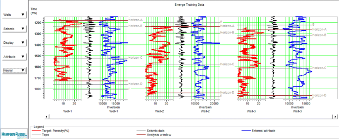

  

  Data imported to the software in the EMERGE section include the chart of the desired parameters from the wells (red), trace around the well (black), and results from inversion around the wells (blue)

• 2. The list of various attributes prepared is given in Table 4:

  Table 4 Part of the seismic attributes is calculated to increase the estimation error for dataset 1

• 3. Table 4 above shows the different attributes along with their error, arranged in order of increasing error. If only one attribute (best attribute) to be used in estimating, the results for the three datasets are as follows. For the porosity estimation in the area, among the three data set, the third set shows the least error. The reason for this high correlation is because of the heterogeneous data in this case,and as a result the error is reduced (Table 5).

  Table 5 The results of applying single-attribute regression on the data

• 4. Multi-attribute analysis: Evaluation of different attributes and attribute designations that will help to increase the accuracy of estimates. Taking 10 attributes and for convolution operator length of 5, the estimation error and validation for the second category data will be as follows:

  With an increasing number of attributes, the correlation of well data with estimations increases, and their general error (black curve) is reduced, which means that by increasing the number of attributes, the existing relationship between the data in the location of the wells is better estimated. The greater number of attributes to mean is the fitness of a polynomial with more order on the data, but after some time, the validation error decreases. The estimation error for other parts of the well increases, and increasing the number of attributes leads to an error in the final result (cubic porosity). This issue can be better explained in Fig. 14. Suppose that the breakers chart is the overall structure of ruling on the entire data, but the dark line is related to more minor structures prevailing on the data in the location of the well. With increasing, excessive attribute to bold curve will be reached, which leads to an error in the estimation.

  Fig. 14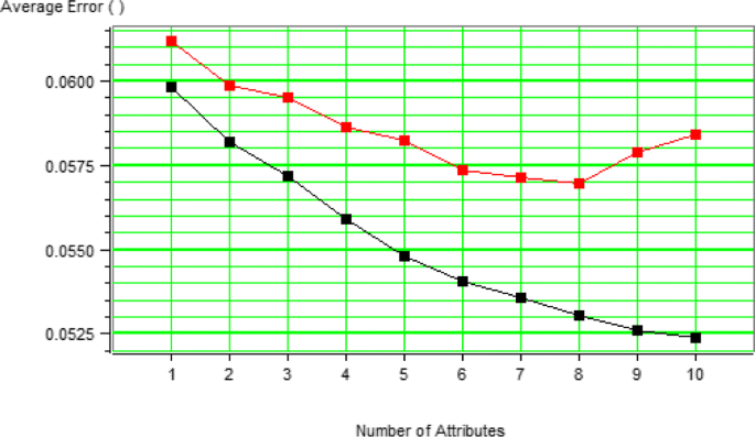

  

  Reason for creating additional error with increasing excessive attributes

  As shown in Fig. 15, for more accurate estimation of porosity in the second category of data, eight attributes are used. This will be done similarly in the other two sets of data.

  Fig. 15

  

  Result of multi-attribute analysis (10 attributes by length operator 5) for the second category of data. The black curve represents total failure, and the red curve represents validation error

• 5. Applying multiple linear regressions attributes and calculates the desired parameters in the well location and verifies correlation.

Now the attributes selected in the previous step are entered into the calculations, and errors in correlation can be checked. The results of the application of multiple linear regression to the attributes are given in Table 6.

Table 6 The results of applying multi-attribute regression on the data

In this case, by changing the convolutional operator length, the number of suitable attributes changes, but the final correlation error does not change significantly. By increasing the length of the convolutional operator, the number of attributes is reduced. For the calculation interval, the number of data in the third category is the lowest, and the number in the first category is the greatest. It can be concluded that whatever desired range be less, because of the reduced heterogeneity of the data, estimation can be performed more easily and accurately. The results obtained by applying this method using selected attributes on the seismic data in the area of the well or the desired reservoir are given in Fig. 16.

Fig. 16

Porosity obtained by applying multi-attribute regression on the second category data at one section and the desired well parameters

As can be seen in Fig. 16, the porosity in the downhole diagram and section estimated with multi-attribute regression shows that this is not a good fit. This is because of the low correlation of this method (0.61) and the lack of sufficient accuracy in the correlation of well and seismic data. The downhole diagram is not on the proper seismic section. This can also be seen in Fig. 17.

Fig. 17

Diagram of estimated porosity versus actual porosity for the second category data using multi-attribute regression

Estimation of porosity using neural networks

Here, we are looking for a nonlinear relationship between the well and seismic data. As mentioned, this goal can be achieved using several algorithms to train the network. Here, three networks, i.e. PNN, MLFN, and RBF, are examined and compared. Eventually, the best network to compare with the other two methods (linear regression and geostatistical) is selected, and is used to estimate the parameters of interest. Neural networks, such as linear regression, the desired parameter in the seismic cube and the form of three-dimensional measures. In this method, in the following order we will act:

• 1. Learning network by using the selected attribute in the previous step and then validation of trained networks:

  Tables 7, 8, and 9 show the results for training and validation of different networks on three available data series (Tables 7, 8, 9).

  Table 7 Results of evaluation of various networks for the first set of data

  Table 8 Results of evaluation of various networks for the second set of data

  Table 9 Results of evaluation of various networks for the third set of data

According to these tables, the PNN network contains the highest correlation for training and validation, and the lowest error. This mainly because of the internal structure of the data. Determining the most appropriate method for the estimation is dependent on the nature and quality of the data. On the other hand, this network requires less time for training and is faster than the other networks trained.

• Applying the trained network to the seismic data and obtaining the porosity cube

  As mentioned above, the PNN network showed the highest correlation for this series of data, and therefore this network was applied to the data, resulting in a section as shown in Fig. 18. Here, even though the network has a high relation (0.83), the porosity in the downhole chart and section estimated was not a good fit. As already mentioned, the main reason for this phenomenon lack of correct matching well data on the seismic section. This phenomenon can also be seen in Fig. 19. If the data well properly and carefully was on the seismic section, trend data from the red line in the figure which has a 450 slope, will follow. But as can be seen, data trends follow from the line with a slope of less (Figs. 20, 21, 22, 23).

  Fig. 18

  

  Porosity obtained from applying multi-attribute regression on the third category data at one section, and the desired well parameter

  Fig. 19

  

  Diagram of estimated porosity versus actual porosity for the data third category by using multi-attribute regression

  Fig. 20

  

  Porosity obtained from the PNN network applied to the second category data at one section, and to the desired well parameters

  Fig. 21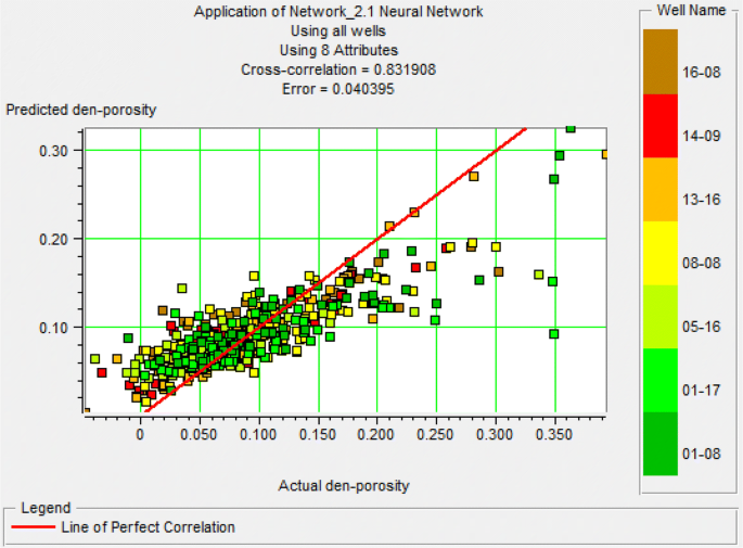

  

  Diagram porosity estimates versus actual porosity for the second category using the network PNN

  Fig. 22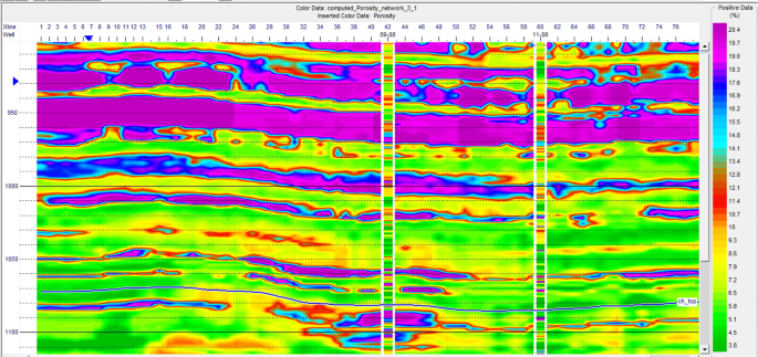

  

  Porosity obtained from the PNN network applied to the third category data at one section and the desired well parameter

  Fig. 23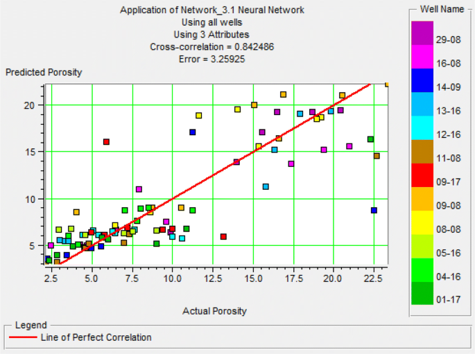

  

  Diagram porosity estimates versus actual porosity for the third category using the network PNN

Estimation of porosity using geostatistical methods

As discussed earlier, with the geostatistical methods we initially examined the spatial structure of the data, and then, using the available data and kriging equations, we estimated the size of the desired parameter in distant parts of the well. We applied these methods as follows:

• Reading the well log data into ISMAP from GeoView

• Variogram modeling (well to well)

Here we examine the spatial structure between well logs. The models fitted to variogram data for the second and third data sets are shown in Fig. 24. As previously mentioned, because the first category of well data is small, the spatial structure cannot be checked, and therefore geostatistical analysis is not applicable for this data category (Fig. 24).

Fig. 24

Variogram obtained from well data for the third category of data

• Applying the ordinary kriging on the well data and estimation of the desired parameter in distant parts of the well (Fig. 25, 26)

  Fig. 25

  

  Porosity obtained from ordinary kriging using structure obtained from well data in the second category

  Fig. 26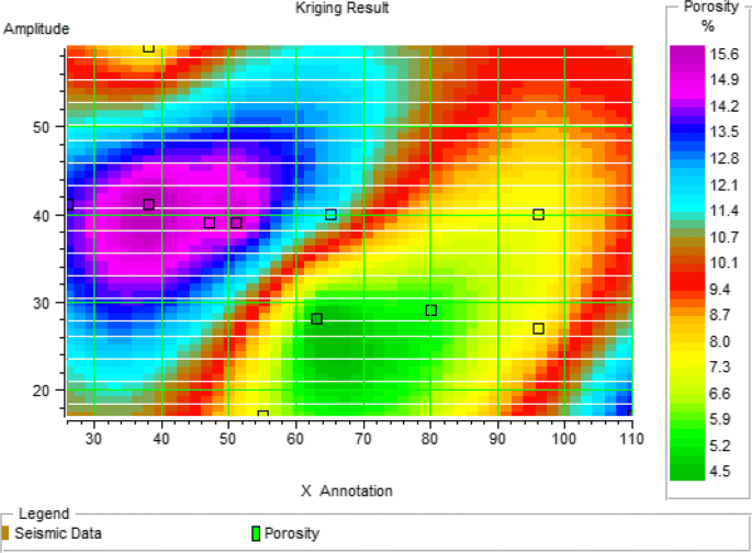

  

  Porosity obtained from ordinary kriging using structure obtained from well data in the third category

At this stage, only data from the well are used for estimation. In fact, we averaged the data from the well in the desired range, and then using the kriging geostatistical estimator, the desired parameter in the other location was obtained. The results for the above two categories of data in the one page are shown in the picture above.

• Reading the seismic data into ISMAP

• Creating data slices

At this stage, seismic indicators will be calculated in the range of data, and attributes in two-dimensional form in the target horizon are obtained, which are used for the following geostatistical analysis.

• Reading data slices into ISMAP, variogram modeling (seismic to seismic), collocated kriging, external drift

At this stage, the two-dimensional attribute calculated in the previous step is checked, and the attribute that is most highly correlated is used for the single-attribute geostatistical estimation (Tables 10, 11).

Table 10 Evaluation of different attributes in the second category

Table 11 Evaluation of different attributes in the third category

The variogram seismic data (seismic to seismic) are now calculated as follows (Figs. 27, 28):

Fig. 27

Spatial structure of the second seismic data

Fig. 28

Spatial structure of the third seismic data

Next, consolidated dependent kriging using the above structure will be calculated. Consolidated dependent kriging is one of a variety of co-kriging methods. It is used when secondary data (seismic) exist in all parts of the grid, such as when three-dimensional seismic data are used (Figs. 29, 30).

Fig. 29

Porosity obtained by dependent kriging using the dominant structure on seismic data in the second category

Fig. 30

Porosity obtained by dependent kriging using the dominant structure on seismic data in the third category

• Multi-attribute analysis

Here, more than one attribute is used, and stepwise regression is employed to selecti the best attributes. The number of the appropriate attributes is selected according to the grid, and a two-dimensional map (EMERGE slice) is obtained (Figs. 31, 32).

Fig. 31

Results of multi-attribute regression for the second category of data

Fig. 32

Results of multi-attribute regression for the third category of data

Now attributes are added to the map obtained in the previous step, and the correlation is verified (Table 12):

Table 12 Verification of correlation attributes by adding multi-attribute analysis in the second category of data

Structural analysis is performed for this new seismic data, and the results are shown in Figs. 33 and 34.

Fig. 33

The structure of the second seismic attributes

Fig. 34

The structure of the second seismic attributes

Then, using the variogram above, conventional kriging is applied to obtain the results shown in Figs. 35 and 36:

Fig. 35

Result of geostatistical estimation of porosity on the one page for the second category of data

Fig. 36

Result of geostatistical estimation of porosity on the one page for the third category of data

As we know, the geostatistical method measures errors in all predicted points. As shown in Fig. 37, prediction error is lowest around the well, and increases with increasing distance from the well. This represents the impact of the spatial structure and the location of the data on the statistical method).

Fig. 37

Map of estimation error distribution

Analysis of results

Now, the three methods are compared with one another in each of the data categories. Estimation error and data correlation for each data set are summarized in Tables 13, 14, and 15. In the first category, geostatistical analysis was found to be the best and most accurate method, and yielded higher correlation and lower estimation error than multi-attribute analysis. In the second data category, the opposite is the case. This may be explained by the small estimation range, and simply the nature of the data. When the relationship of the data is linear, multi-attribute analysis is the best method. Using other methods with this data category leads to the creation of additional errors. Indeed, whether one method is superior to the other dependent on the nature and quality of the data (Figs. 38, 39, 40).

Fig. 38

2D porosity from PNN_dataset2

Fig. 39

2D porosity from multi-attribute_dataset2

Fig. 40

2D porosity from geostatistics_dataset2

Table 13 The results of three different methods for first category data

Table 14 The results of three different methods for second category data

Table 15 The results of three different methods for third category data

As was observed, the neural networks and multi-attribute analysis methods eventually measure the desired parameter in the form of a three-dimensional cube, while the geostatistical method results in a two-dimensional form, shown on one page. To compare these methods, they can be averaged from the porosity cube at the same level the geostatistical analysis has calculated porosity, resulting in the form of two-dimensional and on one page achieved. This is performed by data slicing with the software. Which data at the level of interest does average. As can be seen in Fig. 41, for the third category data, the geostatistical method provides an estimation of the data with greater precision and better quality, especially around wells. However, the maps obtained with the three methods all achieve a good approximation. With regard to the difference between the porosity obtained by the geostatistical method and the other two methods, the porosity estimated by the geostatistical method is about 2% lower than that obtained with the other two methods (Figs. 42, 43)

Fig. 41

2D porosity from PNN_dataset3

Fig. 42

2D porosity from multi-attribute_dataset3

Fig. 43

2D porosity from geostatistics_dataset3

Conclusions

• 1. In the process of computing multiple regression methods, it was found that the use of a greater number of attributes resulted in better correlation of the estimated data with actual data on the location of wells. However, this did not necessarily lead to increased accuracy in data estimation distant from the well and thus the generalizability of the method. Different attributes should thus be reviewed and evaluated in order to select attributes that help to increase the accuracy of estimates in locations remote from wells.

• 2. Attributes used in the estimates must have a physical connection with the desired parameter, and attributes that are unrelated to the desired parameter (such as azimuth or curvature attributes for porosity) should be removed from the list of attributes and analysis.

• 3. Since physically, porosity provides the greatest impact on the density and speed of sound, and as a result acoustic impedance, attributes obtained from the results of seismic inversion are generally best for estimating reservoir parameters, especially porosity. Inversion accuracy will have a large impact on the accuracy of the estimated data, so the seismic inversion operation must be performed carefully and accurately.

• 4. Care must be taken in the matching of well data to the seismic data, because it can have a significant impact on the results, and if is not done correctly, it will lead to differences in the final result.

• 5. The results of linear regression show lower correlation and higher error than the other two methods. In contrast, the neural network approach has a specific equation and correlation coefficient and fixed error. While equations and the nature of the data in the artificial neural network are hidden, and correlation questions with the aim of estimating error are also random and may change each time the program is run, because of the higher compliance with the neural network approach, this method is preferable to multiple regression.

• 6. When the smallest range is used for estimating the desired parameter, because the heterogeneity of the data is reduced, estimation will be easier and more accurate.

• 7. By comparing different neural network approaches, it can be concluded that the neural network PNN using Gaussian functions is the best algorithm to obtain porosity in seismic data volume.

• 8. It is not possible to conclude whether the geostatistical or neural network method is more appropriate for estimation, as the nature and quality of the data will determine whether one or the other is better. Generally, however, considering the spatial structure of the data and the complexity of the geology, geostatistical methods are the most reliable method.

• 9. If the number of wells is small, geostatistical methods may lose their effectiveness. In the geostatistical methods, estimation error is lowest in the local area around the well, and increases with distance from the well.

References

Bahmaei Z, Hosseini E (2019) Pore pressure prediction using seismic velocity modeling: case study, Sefid-Zakhor gas field in Southern Iran. J Pet Explor Prod Technol. https://doi.org/10.1007/s13202-019-00818-y
Brown AR (2001) Understanding seismic attributes. Geophysics 66(1):47–48. https://doi.org/10.1190/1.1444919
Chopra S, Marfurt KJ (2005) Seismic attributes—a historical perspective. Geophysics 70(5):3SO–28SO. https://doi.org/10.1190/1.2098670
Duffaut K, Landrø M (2007) Vp/Vs ratio versus differential stress and rock consolidation-A comparison between rock models and time-lapse AVO data. Geophysics. https://doi.org/10.1190/1.2752175
Duffaut K, Wang Y, Nordskag JI (2018) Estimating horizontal resistivity trends in sedimentary rocks: a case example from the northern north sea. 80th EAGE Conference and Exhibition 2018. https://doi.org/10.3997/2214-4609.201801405
Gholami A, Ansari HR (2017) Estimation of porosity from seismic attributes using a committee model with bat-inspired optimization algorithm. J Pet Sci Eng 152:238–249. https://doi.org/10.1016/j.petrol.2017.03.013
Hampson DP, Schuelke JS, Quirein JA (2001) Use of multiattribute transforms to predict log properties from seismic data. Geophysics 66(1):220–236. https://doi.org/10.1190/1.1444899
Holt Rune M, Bauer A, Bakk A (2018) Stress path dependent velocities in shales: impact on 4D seismic interpretation. Geophysics 83:MR353–MR367. https://doi.org/10.1190/geo2017-0652.1
Hosseini E, Gholami R, Hajivand F (2019) Geostatistical modeling and spatial distribution analysis of porosity and permeability in the Shurijeh-B reservoir of Khangiran gas field in Iran. J Pet Explor Prod Technol 9:1051–1073. https://doi.org/10.1007/s13202-018-0587-4
EMERGE and ISMAP Documentation (2006) Hampson-Russell Software Ltd
Landrø M, Kodaira S, Fujiwara T, No T, Weibull W, Arntsen B (2019) Time lapse seismic analysis of the Tohoku-Oki 2011 earthquake. Int J Greenhouse Gas Control 82:98–116. https://doi.org/10.1016/j.ijggc.2019.01.002
Maity D, Aminzadeh F (2012) Reservoir characterization of an unconventional reservoir by integrating microseismic, seismic, and well log data. In: SPE western regional meeting, 21–23 March, Bakersfield, California, USA. https://doi.org/10.2118/154339-MS
Maity D, Aminzadeh F (2015) Novel fracture zone identifier attribute using geophysical and well log data for unconventional reservoirs. Interpretation 3(3):T155–T167. https://doi.org/10.1190/INT-2015-0003.1
Ogiesoba OC (2010) Porosity prediction from seismic attributes of the Ordovician Trenton-Black River groups, Rochester field, southern Ontario. AAPG Bull 94(11):1673–1693. https://doi.org/10.1306/04061009020
Oliveira MR, Ribeiro N, Johann PR, Camarao LF, Steagall DE, Kerber P, Carvalho MJ (2005) Using seismic attributes to estimate porosity thickness in “pinch-out” areas. In: SPE Latin American and Caribbean petroleum engineering conference, 20–23 June, Rio de Janeiro, Brazil. https://doi.org/10.2118/94913-MS
Pramanik AG, Singh V, Vig R, Srivastava AK, Tiwary DN (2004) Estimation of effective porosity using geostatistics and multiattribute transforms: a case study. Geophysics 69(2):352–372. https://doi.org/10.1190/1.1707054
Russell BH, Lines LR, Hampson DP (2003) Application of the radial basis function neural network to the prediction of log properties from seismic data. Explor Geophys 34(2):15–23. https://doi.org/10.1071/EG03015
Somasundaram S, Mund B, Soni R (2017) Seismic attribute analysis for fracture detection and porosity prediction: a case study from tight volcanic reservoirs, Barmer Basin, India. Lead Edge 36(11):947b1–947b7. https://doi.org/10.1190/tle36110947b1.1
Van Riel P (2000) The past, present, and future of quantitative reservoir characterization. Lead Edge 19(8):878–881. https://doi.org/10.1190/1.1438735
Yan H, Dupuy B, Romdhane A, Arntsen B (2018) CO2 saturation estimates at Sleipner (North Sea) from seismic tomography and rock physics inversion. Geophys Prospect 67(4):1055–1071. https://doi.org/10.1111/1365-2478.12693
Acknowledgements
We are grateful to the Sarvak Azar Engineering and Development (SAED) Company and Oil Industries Engineering and Construction Group (OIEC) for financial support.
Author information
Authors and Affiliations
Corresponding author
Rights and permissions
Open Access This article is licensed under a Creative Commons Attribution 4.0 International License, which permits use, sharing, adaptation, distribution and reproduction in any medium or format, as long as you give appropriate credit to the original author(s) and the source, provide a link to the Creative Commons licence, and indicate if changes were made. The images or other third party material in this article are included in the article's Creative Commons licence, unless indicated otherwise in a credit line to the material. If material is not included in the article's Creative Commons licence and your intended use is not permitted by statutory regulation or exceeds the permitted use, you will need to obtain permission directly from the copyright holder. To view a copy of this licence, visit http://creativecommons.org/licenses/by/4.0/.
About this article
Cite this article
Soleimani, F., Hosseini, E. & Hajivand, F. Estimation of reservoir porosity using analysis of seismic attributes in an Iranian oil field. J Petrol Explor Prod Technol 10, 1289–1316 (2020). https://doi.org/10.1007/s13202-020-00833-4
Received:
Accepted:
Published:
Issue Date:
DOI: https://doi.org/10.1007/s13202-020-00833-4