VSP polarization angles determination: Wysin-1 processing case study

Abstract

In this paper, we present an analysis of borehole seismic data processing procedures required to obtain high-quality vertical stacks and polarization angles in the case of walkaway VSP (vertical seismic profile) data gathered in challenging conditions. As polarization angles are necessary for more advanced procedures like anisotropy parameters determination, their quality is critical for proper media description. Examined Wysin-1 VSP experiment data indicated that the best results can be obtained when rotation is performed for each shot on data after de-noising and vertical stacking of un-rotated data. Additionally, we proposed a procedure of signal matching that can substantially increase data quality.

Introduction

Obtaining more accurate geological information based on the analysis of seismic waves is now even more important than it was in the past. 3C VSP walkaway seismic survey can refine surface seismic observations, provide additional information about the geology (Hinds et al. 1996; Trela 1999), and ultimately allow one to obtain complete information on the anisotropic elasticity tensor (Dewangan and Grechka 2003). Additionally, it gives the possibility of obtaining a high-quality seismic section in the domain of a common depth point. This is due to the fact that the seismic signal propagates through the geological media in such a way that there is only one passage through the low-velocity zone (LVZ). This zone, due to the often high variability of its components, a small compaction, and usually a large amount of pore space, has a significant impact on the energy of seismic waves. This is caused mostly because of energy dissipating on inhomogeneities and by using it for surface waves generation. Additionally, seismic borehole surveys greatly reduce the impact of spherical divergence and energy attenuation as a result of non-elastic interactions (Trela 1996a, b; Gulati et al. 2004; Kuzmiski et al. 2009). Walkaway VSP surveys also improve the accuracy of microseismic observations by helping in the proper determination of perforation parameters for hydraulic fracturing in shale formations (Pei et al. 2017). Developing an optimal technique for walkaway VSP data processing will consequently allow for the minimization of errors and the maximization of the signal-to-noise ratio. It is a key factor for correct interpretation and application of these data for hydrocarbon exploration.

In the case of a classic, near-offset 3C VSP survey, it is assumed that each of the receiver’s components registers only one type of medium vibrations. Obviously, this assumption is only true if the medium is isotropic and homogeneous. Vertical component Z measures longitudinal wave, while horizontal components H1 and H2 record transversely or longitudinally polarized transverse waves. In the case of a multi-level borehole receiver tool (like 96-channel BSR Slimhole Array System used in Wysin-1 experiment), the walkaway VSP allows obtaining detailed seismic information at a given depth in a function of the offset. This type of measurement allows one to obtain a better quality seismic signal (Payne et al. 1994; Bartoń 2014) and more detailed information about seismic attenuation (Xu et al. 2001). Eventually, high-quality VSP allows one to obtain accurate information about local anisotropy (Dewangan and Grechka 2003; Grechka and Mateeva 2007) and deposit parameters (Xiang-e et al. 2009).In this case study considering Wysin-1 VSP experiment, we examine processing sequences that allows the most efficient vertical stacking and, in consequence, stabile azimuth and inclination angles determination with limited errors. Accurate determination of both polarization angles or, with some assumptions, only inclination in every receiver is a critical factor for the estimation of local anisotropy by using P wave only inversion (Grechka and Mateeva 2007).

Our motivation for this study was twofold. First of all, we wanted to get the most accurate values of inclination for the P wave only inversion of the transverse isotropy medium observed in some layers around Wysin-1 well. Secondly, an additional issue was the very challenging and unusual data acquisition field conditions. The profile line was localized mostly in farmlands, and the acquisition was done after heavy rain, which heavily affected data quality (Fig. 1).

Fig. 1

Examples of field condition during acquisition. From the beginning of October, up to the time of acquisition (November), as well as during them, there were significant rainfalls, which resulted in very difficult terrain conditions. The ground was soaked with water. This caused the vibroseis to sink into the soaked ground during sweeping. There were more than one sweep on each point, and a significant change of the geotechnical conditions occurred in the surface zone between sweeps. It was our motivation to perform a new approach for data processing (photo credit: unpublished materials of Geofizyka Toruń SA)

We took under consideration signal matching for every SP separately before performing the vertical stacking of records. Finally, we wanted to point out the most practical position for polarization analysis in the processing sequence.

In this study, we use signal-to-noise ratio in a function of offset and depth as a quantitative evaluation criterion, as well as the error values for determining the inclination angles for individual depth levels. As an additional qualitative criterion, we used the quality of the seismic record in the common shot-point domain. The analyzed data were gathered in the Liniewo area in the Pomeranian Voivodship. The seismic survey was carried out by the company Geofizyka Toruń SA on behalf of the Department of Geology, Geophysics and Environmental Protection of the AGH University of Science and Technology in Kraków, as part of the “Polish Technologies for Shale Gas” project.

The characterization of acquisition and region

Data were acquired in Northern Polish village of Wysin situated in the Peri-Baltic Syneclise. Two horizontal wells and one vertical well were drilled (see Fig. 2). In the vertical Wysin-1 well, a walkaway VSP survey was conducted. It is morphologically a varied area localized within river valleys, lake gutters, and moraine uplands.

Fig. 2

Localization of Wysin-1 well (yellow dot), Wysin 2H and 3H wells (green line) and profile of sources (red line) with source 15 (black dot)

The profile was carried out in accordance with the trajectory of the Wysin-2H and Wysin-3H horizontal wells in which the hydraulic fracturing tests and microseimic monitorings were performed. In the Wysin-1 well, the acquisition was carried out using the 96-receiver 3C BSR Array System (Oyo Geospace Company). Channel distance intervals were 15 m, which made it possible to measure from 2400 (depth of #1 receiver) to 3825 m (depth of #96 receiver) MDGL (measured depth from ground level) zone simultaneously. Receivers were located mostly in Upper Silurian and Wenlock rocks (see Fig. 3). It allowed the study of the characteristics of the seismic signal (in case of polarization angels values determination) passing through the highly attenuating rocks of Zechstein—the black colored layer in Fig. 3. The recording time was 4 s, and the length of the sweep of the vibrating groups was 16 s. The frequency range of the sweep was 6–140 Hz. At total of 480 shot points were localized on the profile with 25-m intervals, which allowed obtaining the maximum offset equal to 12 km. On each source point (SP), the waves were generated from two up to eight times.

Fig. 3

Interval velocity model with WYSIN-1 well trajectory (yellow line) and receiver location: from the shallowest receiver No. 1 to the deepest receiver No. 96. Zechstein complex is colored black

Walkaway VSP acquisition and wavefield separation

Typical acquisition of walkaway VSP consists of receivers (mostly geophones) located in the vertical well and surface sources (dynamite or vibroises). Walkaway geometry includes multiple source location (near, middle, and far offsets) along the profile (Fig. 4) which can be compared with a 2D seismic line. The geometry of source positions can also be performed in a 3D surface grid. This kind of seismic survey allows one to record downgoing waves and upgoing waves (reflected from particular seismological layers, and they can be used together with reflection seismic data) (Hinds et al. 1996).

Fig. 4

Typical acquisition scheme of multicomponent walkaway VSP with components rotation steps. The acquisition consists of N_S surface sources (yellow triangles) and N_R receivers (3-C geophones) for the multicomponent tool. For VSP measurements, OFFSET refers to the distance from the well center to the source. The receivers’ depth levels measured from the well top are in meters MDGL (measure depth from ground level). The red coordinate system corresponds to the real northward, eastward, and true vertical depth. The blue ones correspond to the receivers’ components H1, H2 (horizontal plane), and V1 (vertical), which can take random positions on each depth level. To maximize energy of the direct wave, the horizontal rotation is performed first to relocate the configuration with angle ϕ, after that, the vertical rotation is performed with angle θ. The presented ray paths are not straight lines, because of the velocity gradient in the presented layer

Typically, receivers in the borehole are 3-C geophones. When the well is vertical, axis Z is perpendicular to the component V (vertical) axis, and components H1 and H2 axes can be in a random position in the horizontal plane. The angle between H1 and H2 is always 90°. One of the important steps in walkway VSP processing is to isolate the downgoing P wave energy (Hinds et al. 1996). Hardage (1985) proved that SH and SV propagate along with a downgoing P wave path.

The idea of the wavefield separation for the compression P wave and longitudinal SV and SH waves is based on the analytical method of the determination of the medium particles’ direction of motion (Galperin 1984).

The typical procedure operates on the energy of the downgoing P wave that first breaks in the selected time window. Data from horizontal components (X and Y) are plotted on the hodogram for each time sample in the analysis window (Hardage 1985). The length of the window should always be tested, regardless to previous experience, and it should include the energy of first breaks. The noise level, first-breaks energy, and S/N ratio should be considered when choosing the window. Normally, the ellipse with the longer axis pointing to the source direction is obtained (Fig. 5).

Fig. 5

The concept of hodogram analysis is in 3-C borehole seismic observation. The samples from the selected time window are plotted on the graph according to their amplitude. Depending on the form, they are creating on the graph (circle, ellipse), after numerical match, and the rotation angle can be estimated according to the symmetry axis

After that, the reorientation of components is performed according to estimated angles. As the final result, energy is maximized on the V component, and the energy which was not possible to obtain on V component is projected on the H1 and the rest of the energy is stored in H2 component. In this paper, the method of wavefield separation proposed by DiSiena et al. (1984) was applied and expanded upon. The final rotation effect of all three components was compared depending on three methods of the component’s rotation angles calculation: peak vector amplitude, maximum power search methods, and the principal component method (compare—Kirlin and Done 1999).

Peak vector amplitude (PVA) is a method based on the analysis of the magnitude vector for a given time sample. Please note that, in this approach, the word “magnitude” cannot be directly related to the seismological definition. For the needs of seismic surveys, the magnitude vector for a given time series t_n in the interval $\varTheta = (n_{a} ,n_{z} ),\;n_{a} < n_{z} \,\varLambda \,n$ belongs to Θ and will be defined as the supremum of the sum of squares of amplitudes in the range Θ for all registered components on given time samples belonging to Θ. In this method, the angle of rotation is determined based on the direction of the maximum amplitude vector, on the basis of the time point t_x found in the window Θ in the way described above.

Maximum power search (MPS) is a method of finding a new coordinate system in which components get maximized energy. The proposal coordinates system differing from the initial position by the angle δ_n are defined using a Δδ step. Then, for each new position, the energy maximum values for each axis are calculated based on the samples in the given time window. The final step in the procedure is to choose a system that gives maximum energy for the determined inclination and azimuth.

Principal component method (PCM) is based on the analysis of linear space endomorphism, and it is a widely used technique in statistics (Scheevel and Payrazyan 1999; Hoteling 1933). In a given time window, along each of the three mutually perpendicular axes, the measured values can be treated as an energy representation of an object in this space. For all points, eigenvectors and eigenvalues are calculated. These vectors are then used to determine the average displacement direction and its polarity. For a better understanding of this method, consider the situation shown in Fig. 5. The input of this method is a matrix of N-dimensional vectors. The dimension of each vector is related to the dimension of the pre-chosen sampling window. Chosen samples should be a representative population of considered event (Scheevel and Payrazyan 1999). When the cloud of the points on the histogram could be described with an ellipse, its longer axis is a polarization direction of the considered wave. Consider the N realization of particular vector samples as $\gamma$. To determine the average value, Eq. (1.0) is used (after Michaels 2001)

$$ \bar{\gamma } = \frac{1}{N}\sum \gamma_{j} = \left( {\begin{array}{*{20}l} {\overline{{H1_{i} }} } \hfill \\ {\overline{{H2_{i} }} } \hfill \\ \end{array} } \right), $$

(1.0)

where H1_i and H2_i represent samples from two orthogonal components.

However, in the N-dimensional vector space, the scalar inner product of the vectors created by N realizations of the seismic sample can be defined as follows:

$$ \left\langle {H1,H2} \right\rangle = \sum {\underline{H1}_{i} H2_{i} = H1^{\text{T}} H2} $$

(2.0)

As the final step, the covariance matrix (MC) is created, where eigenvectors with largest values correspond to the polarization direction:

$$ {\text{MC}} = \sum {\left( {\gamma_{j} - \bar{\gamma }} \right)\left( {\gamma_{j} - \bar{\gamma }} \right)}^{\text{T}} = \left[ {\begin{array}{*{20}c} {\left\langle {\left( {H1 - \overline{H1} } \right),\left( {H1 - \overline{H1} } \right)} \right\rangle } & {\left\langle {\left( {H1 - \overline{H1} } \right),\left( {H2 - \overline{H2} } \right)} \right\rangle } \\ {\left\langle {\left( {H2 - \overline{H2} } \right),\left( {H1 - \overline{H1} } \right)} \right\rangle } & {\left\langle {\left( {H2 - \overline{H2} } \right),\left( {H2 - \overline{H2} } \right)} \right\rangle } \\ \end{array} } \right] $$

(3.0)

For more information about this method with its mathematical and historical background, see Jolliffe (1986).

Analyzing the records shown in Fig. 6, it can be concluded that the worst quality effects (in the case of the vertical component record) are produced by the MPS method. It can be noticed especially on receivers located at the deeper levels where the energy of the longitudinal wave has not been properly separated and expressed on the vertical component. In consequence, weaker longitudinal wave energy is observed on this component. The difference between two other methods, PCM and PVA, is hard to notice in the case of longitudinal waves. In this paper, we are focused especially on P wave energy, so we decided to use the PCM method in further studies, because it gives slightly more balanced results and provides a better energy representation of P wave first breaks.

Fig. 6

Comparison of three methods of wavefield separation

Noise attenuation and vertical stacking

The amplitude and hence the signal strength is influenced by many different factors—from the acquisition itself through the features of the geological media, the non-stationarity of the seismic signal, to the phenomena like interference and noise (Varela et al. 1996; Kowalski 2016).

In the first stage of data processing, we were focused on the determination of which stage of VSP processing the rotation of the components should be applied to obtain the most accurate and stable values of polarization angles. Please note that these values are critical for anisotropy determination using P waves (Grechka and Mateeva 2007). Four possible options were considered:

• OPTION 1 (O1): rotation is performed on raw data, before vertical stacking for each shot separately. Then vertical stacking and de-noising are applied.

• OPTION 2 (O2): rotation is performed on raw data after vertical stacking, and then de-noising is applied.

• OPTION 3 (O3): rotation is performed on data after de-noising, which is performed for each shot separately, and then vertical stacking is performed.

• OPTION 4 (O4): rotation is performed for each shot on data after de-noising and vertical stacking of un-rotated data.

The analyses were performed for different offsets for each of the 96 depth levels. Vertical stacking aims to increase the efficiency of the source output, eliminate some random interferences, increase the signal-to-noise ratio, and provide data reduction (for more details see Klemperer 1987; Kumar and Sinha 2008). The signal-to-noise ratio results for shot point 15 obtained for all options are presented in Fig. 7 for the vertical component and in Fig. 8 for the horizontal component (H1). It is clearly visible that the implementation of the procedures aimed at getting rid of unwanted parts of signal for each registration should be performed before the rotation of the individual components.

Fig. 7

S/N ratios for vertical components: O1 (blue), O2 (red), O3 (yellow), and O4 (green)

Fig. 8

S/N ratios for horizontal component H1: O1 (blue), O2 (red), O3 (yellow), and O4 (green)

De-noising part of presented sequence included the following procedures:

• 1. Perform band-pass filtering using a single, zero-phase, and a single time-invariant Ormsby filter (16 to 80 Hz pass-band filter with a 8 Hz wide low-cut ramp and a 40 Hz wide high cut ramp).

• 2. Remove mono-frequency noise (which were frequent for the analyzed registrations) on the basis of determining the mean of the arrhythmic value of such disturbance along a single seismic trace (this kind of noise is connected with tool generated harmonic noise).

• 3. Provide frequency filtration based on time–space analysis of the record using a short-time Fourier transform (STFT) with replacing disturbance, connected to surface noise transmitted by a cable or the tool resonance noise, using values calculated on the basis of neighboring traces that were considered as undisturbed. (The time window was 200 ms long and has the five traces aperture. Those traces are used to calculate the median spectral amplitude when the threshold amplitude on particular sample has been reached. Threshold multiplier values were set on 3. The frequency of interest for STFT was 20–80 Hz.)

• 4. Provide the suppression of high-energy noise using horizontal and vertical median filtration. [The length of the vertical median computation window was 100 ms, and the width of horizontal median computation window was 30 traces. The 50 ms length cosine taper zone has been used with no scaling factor. This kind of noise can be inducted by tool slippage due to weak anchorage and tube waves (which are a problem only for near-offset shot points).]

• 5. Top mute the energy over first breaks.

  (Some types of noise (like tool resonance) are normally removed by moving the tool to another location; however, in this specific case, the tool had not been moved up during the whole acquisition. Moreover, in some parts of the well, there was no casing between the inner and outer tube, which leads to the generation of additional noise. When the casing is unbounded, the ring noise can be present too. It has to be notice that the last receivers are hanging on the cable of a length over 3 km. If the anchorage is not perfect, the various forces have an effect on receivers and could lead to unexpected noise generation that is hard to classify. The results of the described procedures are shown in Fig. 9.)

  Fig. 9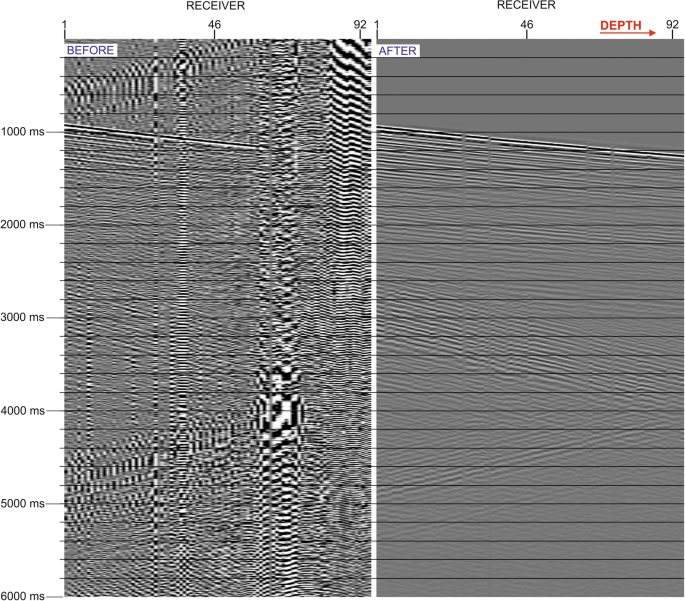

  

  The rotation efficiency mostly depends on first-break signal quality. It is obvious that the first-break identification and separation is critical for the rotation procedure

Figure 10 shows the average values of the calculated inclinations, and Fig. 11 shows the average values of the calculated azimuths obtained using the PCM method. The differences in inclination results for analysis options are relatively large, but it is clearly visible that the results obtained for O3 and O4 are more stable and obtained with lower errors. Errors for particular receiver σ(R_i) have been calculated as a combination of standard deviations of the receivers group of five (N = 5) according to Eq. 4.0:

$$ \sigma (R_{i} ) = \sqrt {\frac{{\sum\nolimits_{i}^{N} {\left( {R_{i} - \bar{R}} \right)^{2} } }}{N}} $$

(4.0)

Errors for the complete measure depths for each shot point (SP) are calculated as an arithmetic average of standard deviation for all angle estimations at particular depths according to Eq. 5.0:

$$ \sigma ({\text{SP}}) = \frac{{\sum\nolimits_{i}^{{N_{E} }} {\sigma (R_{i} )} }}{{N_{E} }}, $$

(5.0)

where N_E number of estimated angles with σ(R_i) < 5° (for inclination) and σ(R_i) < 15° for azimuth; σ(SP) average error of inclination or azimuth estimation for each SP.The average value of error is 1.56 for O4, and it is equal to 7.06 for O1. In the case of analyzed registrations induced at the offset of 3200 m from the well and for the middle receiver located at a depth of 3000 m, the + 8% error in determining the angle causes the 750 m (24%) shift in hypothetical source location. However, the analogous test for O3 shows the difference at the level of 16 m (0.5%), and for O4, 8 m (0.25%), according to the result obtained from ray tracing.

Fig. 10

Comparison between average values of inclination determined for data processed in O1, O2, O3, and O4 with error bars (black lines)

Fig. 11

Comparison between average values of azimuths determined for data processed in O1 (blue), O2 (orange), O3 (gray), and O4 (yellow)

We took depth interval between receivers 26 and 31 under more specific examination, because of a substantial change in the quality of inclination values and their trend compared to neighboring receivers for all options (Fig. 12). For O1, the inclination values in this area are stable when others are much more chaotic; however, the opposite situation is noticeable for O2. Additionally, for O3, the increasing trend of inclination from receiver 5 to 26 can be seen, and there is an almost constant inclination value from receiver 31 to 41. It is surprising that, from receivers 26 to 31, inclination values are decreasing, and, between receiver 31 and 32, the rapid change is visible (over 5°). For O4, the inclination between receivers 26 and 31 seems to be stable; however, the distribution of changes can be approximated by a second-degree polynomial curve. In Fig. 10, the comparison between average inclination values and average error values for the mentioned interval is shown.

Fig. 12

Average values (receivers 26–31) of inclination for O1, O2, O3, and O4 with average error (orange line)

It is easily noticeable that error and inclination values for O1 and O2 are significantly higher than for O3 and O4. At this stage, we chose O4 as the best option for most accurate polarization angle determinations; however, the expectation was that the course of changes will continue the increasing trend or will be stable instead of changes that can be described by a second-degree polynomial curve. In the next step, the novel signal processing has been added to exclude the described abnormal trend of changes in the behavior visible in O4 result.

Signal matching

The analyses were carried out on data processed according to the O4 scheme. Additionally, in the case of testing high-resolution walkaway VSP made in difficult terrain conditions with high soil moisture, the issue of time–frequency matching of the signal of individual shots to each other also seems to be significant. To analyze possible impact of this procedure on polarization evaluation results, we performed it for data processed using O4 scheme. Before vertical stacking, we have to ensure that the individual elements entering the stacking process will certainly strengthen the useful signal and attenuate the noise and random interference. It is obvious that, between the first and last sweep, the geotechnical conditions in the surface zone may significantly change, especially in the case of high humidity and poor consolidation. In order to determine whether matching the signal of individual sweeps to each other is necessary, a similarity analysis of the records was performed for each sweep with respect to base record which is the average of all registrations for shot point No. 15. Then, cross-correlation was calculated between the trace from the given sweep and the base trace (Fig. 13). Analysis of the correlation coefficients shows a significant increase in similarity for receivers over depth. What is important is that a significant drop of correlation values is noticeable for receivers 26–31 (discussed before) for all six sweeps. As visible for sweep No. 3, the lowest possible values are observed.

Fig. 13

Correlation between base record and particular sweeps

It is possible that the observed phenomena are due to fact that the well was not properly cased in the depth interval above the 41th receiver. The observed effect of changes in the correlation values may be related to the changes in the quality of the receivers’ anchorage or some near well effects and geology itself. However, at this stage of the study, it is hard to fully explain that effect. Another reason for existing differences between vertical and horizontal components can be explained by the fact that only P wave was transmitted from source and most energy observed on horizontal components is transmitted through converted waves. A drastic decrease in correlation coefficients observed for selected receivers (e.g., 6, 22, 33) is most probably due to waddle anchorage.

In order to evaluate whether the evaluation of matching is necessary, we had to create a proper criterion. We created it using pilot traces and the L2 norm calculated between the pilot and all traces. It is clearly visible that signal matching helped to stabilize values of inclination and azimuth over depth (Figs. 14 and 15). The average evaluation error decreased about 33% (for inclination) and about 15% (for azimuth). Figure 16 shows the comparison of the S/N ratio (SP 15) for each trace before and after the procedure described above.

Fig. 14

Comparison of inclination values for O4 before signal matching (orange dots) and after signal matching (blue dots)

Fig. 15

Comparison of azimuth values for O4 before signal matching (orange dots) and after signal matching (blue dots)

Fig. 16

S/N ratio for vertical component: before signal matching (blue) and after signal matching (orange)

It is clearly visible that, on some receivers, it was possible to obtain up to 25% higher S/N ratios (Fig. 16) and consequently obtain a better estimation of polarization angles (Fig. 14, Fig. 15).

To validate the obtained results, estimated inclination values after signal matching for different offsets were compared and examined (see Fig. 17). The values of inclination and errors change according to expectations (increasing with offset). The trend of changes between offset is visible, especially for offsets at 2000 and 3000 m. Moreover, it corresponds to the lithology changes. Unfortunately, inclination values for offsets over 4 km show significant changes in the values of the determined angles along the tested well section. It is due to very unusual surface conditions, which reduce the signal strength, and to the high-velocity Zechstein zone that is located between two low-velocity zones.

Fig. 17

Values of inclination for different offsets obtained for O4 after signal matching. Black dots: OFFSET 300 m, average error (AVR ERROR) 0.46, orange dots: OFFSET 1000 m, AVR ERROR 0.78, gray dots: OFFSET 2000 m, AVR ERROR 0.79, blue dots: OFFSET 3000 m, AVR ERROR 1.05, yellow dots: OFFSET 4000 m, AVR ERROR 2.73

In the end, we correlated values of inclination and azimuths (for O4 with signal matching for SP 15 which offset is 3000 m) with lithological complexes of Silurian rocks determined on the basis of well-logs (Fig. 18). The changes are strongly related to lithology with high accuracy. Even very thin layers (C2 and C10) are related to inclination and azimuth values. However, in complex C3, the high variability of determined angles values is noticeable. It can be caused by anisotropy, i.e., the layer can be lithological consistent, but inconsistent in the case of elastic properties. The same situation is noticeable in complexes C6 and C8.

Fig. 18

Values of inclination (blue dots) and azimuth (orange dots) with lithological complexes (C1–C11). Complexes with significant drop of SWE (water saturation factor), increase in PHIE (effective porosity), and TOCW = 05% (total organic carbon) are marked with red squares

Conclusion

This paper examined how walkway VSP data processing affects vertical stacking and polarization angle determination. It was shown that proper data processing can significantly increase the quality of results. Finally, the following conclusions can be made:

• 1. The order of four main procedures is critical for proper polarization angle evaluation based on a three component walkaway VSP survey. In this paper, we have shown that the best results can be obtained when rotation is performed for each shot on data after de-noising and vertical stacking of un-rotated data (Option 4).

• 2. In the case of repeated shots at a given shot point, in conditions of high humidity and ground instability, the calculation and application of the signal matching filter based on pilot registration, being a static representation of all shots at the particular shot point, are justified.

• 3. The matching filter should be calculated and applied after the noise is removed.

• 4. Obtained values are strongly related to lithological complexes (determined on well-logs results).

• 5. There are changes in inclination and azimuth values within particular lithological complex that are not related to the lithology. It is likely that this phenomenon is caused by the elastic inconsistency of a particular complex.

References

Bartoń R (2014) Determination of directional velocity changes of transverse waves in near-wellbore zone based on VSP 3C. Nafta Gaz 70(8):483–492
Dewangan P, Grechka V (2003) Inversion of multicomponent, multiazimuth, walkaway VSP data for the stiffness tensor. Geophysics 68(3):1022–1031. https://doi.org/10.1190/1.1581073
DiSiena JP, Gaiser JE, Corrigan D (1984) Horizontal components and shear wave analysis of three-component VSP data. In: Toksoz N, Stewart RR (eds) Vertical seismic profiling: advanced concepts, vol 15 B. Geophysical Press, London
Galperin EI (1984) The polarization method of seismic exploration. Springer, Dordrecht
Grechka V, Mateeva A (2007) Inversion of P wave VSP data for local anisotropy: theory and case study. Geophysics 72(4):69–79. https://doi.org/10.1190/1.2742970
Gulati JS, Stewart RR, Parkin JM (2004) Analyzing three-component 3D vertical seismic profiling data. Geophysics 69:386–392. https://doi.org/10.1190/1.1707057
Hardage BA (1985) Vertical seismic profiling, 2nd edn. Geophysical Press, London
Hinds CR, Anderson LN, Kuzmiski DR (1996) VSP interpretative processing. Society of Exploration Geophysicist, Tulsa. https://doi.org/10.1190/1.9781560801894
Hoteling H (1933) Analysis of a complex of statistical variables into principal components. J Educ Psychol 24:417–441
Jolliffe (1986) Principal component analysis. Springer, New York
Kirlin LR, Done JW (1999) Covariance analysis of seismic signal processing. Society of Exploration Geophysics, Tulsa. https://doi.org/10.1190/1.9781560802037
Klemperer S (1987) Seismic noise-reduction techniques for use with vertical stacking: an empirical comparison. Geophysics 52(3):322–334. https://doi.org/10.1190/1.1442306
Kowalski H (2016) Inverse Q filtering build into the pre-stack depth migration. Prace Naukowe INiG-PIB, Kraków, p 209
Kumar L, Sinha DP (2008) From CMP to CRS: an overview of stacking techniques of seismic data. In: 7th Biennial international conference and exposition on petroleum geophysics, p 414
Kuzmiski R, Chartes B, Galbraith M (2009) Processing considerations for 3D VSP. Recorder 34(04):31–40
Michaels P (2001) Use of principal component analysis to determinate down-hole tool orientation and enhance SH-waves. JEEG 6(4):175–183. https://doi.org/10.4133/JEEG6.4.175
Payne MA, Eriksen EA, Rape TD (1994) Considerations for high-resolution VSP imaging. Lead Edge 14:173–180
Pei D, Carmichael J, Zhou R, Knapo G (2017) Enhanced microseismic anisotropic velocity optimization by check-shot and walkaway VSP. SEG technical program expanded abstracts, pp 2867–2871. https://doi.org/10.1190/segam2017-17538927.1
Scheevel JR, Payrazyan K (1999) Principal component analysis applied to 3D seismic data for reservoir property estimation. In: SPE technical conference and exhibition. Society of Petroleum Engineers Inc., SPE 56734
Trela J (1996a) VSP data processing. Nafta Gaz 8
Trela J (1996b) VSP data acquisition. Nafta Gaz 5
Trela J (1999) 3-C VSP data processing. Wavefields separation using polarization method. Nafta Gaz 3:1999
Varela LC, Rosa A, Ulrych T (1996) VSP data processing. Nafta Gaz 8
Xiang-e S, Yun L, Jun G, Desheng S, Jixiang L (2009) Anisotropic parameter estimation based on 3D VSP and full azimuth seismic data. SEG technical program expanded abstracts, pp 4105–4109. https://doi.org/10.1190/1.3255728
Xu C, Stewart RR, Osborne AC (2001) Walkaway VSP processing and Q estimation: Pikes Peak, Sask. In: CSEG annual conference
Acknowledgements
We express our gratitude to Jerzy Trela (Director of Geophysics in GT Services) for assistance with VSP processing and interpretation problems. We also thank Michal Podalak (former R&D Department Chief in GT Services) and Henryk Kowalski (R&D Chief in GT Services) for their help, critical remarks, and constructive comments. Additionally, we thank PGNiG S.A. for allowing us to use seismic and well-log data acquired as a part of the project “Polish technologies for shale gas.”
Author information
Authors and Affiliations
Corresponding author
Rights and permissions
Open Access This article is distributed under the terms of the Creative Commons Attribution 4.0 International License (http://creativecommons.org/licenses/by/4.0/), which permits unrestricted use, distribution, and reproduction in any medium, provided you give appropriate credit to the original author(s) and the source, provide a link to the Creative Commons license, and indicate if changes were made.
About this article
Cite this article
Zaręba, M., Danek, T. VSP polarization angles determination: Wysin-1 processing case study. Acta Geophys. 66, 1047–1062 (2018). https://doi.org/10.1007/s11600-018-0200-8
Received:
Accepted:
Published:
Issue Date:
DOI: https://doi.org/10.1007/s11600-018-0200-8