Energy harvesting through arterial wall deformation: design considerations for a magneto-hydrodynamic generator

Abstract

As the complexity of active medical implants increases, the task of embedding a life-long power supply at the time of implantation becomes more challenging. A periodic renewal of the energy source is often required. Human energy harvesting is, therefore, seen as a possible remedy. In this paper, we present a novel idea to harvest energy from the pressure-driven deformation of an artery by the principle of magneto-hydrodynamics. The generator relies on a highly electrically conductive fluid accelerated perpendicularly to a magnetic field by means of an efficient lever arm mechanism. An artery with 10 mm inner diameter is chosen as a potential implantation site and its ability to drive the generator is established. Three analytical models are proposed to investigate the relevant design parameters and to determine the existence of an optimal configuration. The predicted output power reaches 65 μW according to the first two models and 135 μW according to the third model. It is found that the generator, designed as a circular structure encompassing the artery, should not exceed a total volume of 3 cm³.

Appendices

Appendix 1

Fung [7] studied the energy balance over a vessel segment delimited by an inlet and an outlet station (denoted below by indices 1 and 2, respectively). If gravitational forces, heat exchange with the surrounding tissues, as well as heat generation due to viscous losses in blood are neglected, the energy balance reads (in a cylindrical coordinate system {r, φ, z}):

$$ \int\limits_{{A_{1} }} {pu_{z} {\text{d}}A} - \int\limits_{{A_{2} }} {pu_{z} {\text{d}}A} + \int\limits_{S} {{\mathbf{T}} \cdot {\mathbf{u}}{\text{d}}A} = \int\limits_{{A_{2} }} {\tfrac{1}{2}\rho \,q^{2} u_{z} {\text{d}}A} - \int\limits_{{A_{1} }} {\tfrac{1}{2}\rho \,q^{2} u_{z} {\text{d}}A + } \int\limits_{S} {\tfrac{1}{2}\rho \,q^{2} u_{\it{r}} {\text{d}}A} + \int\limits_{V} {{\partial \mathord{\left/ {\vphantom {\partial {\partial t}}} \right. \kern-\nulldelimiterspace} {\partial t}}\left( {\tfrac{1}{2}\rho q^{2} } \right){\text{d}}V} $$

(23)

$$ \begin{array}{*{20}c} {{\text{{\bf{u}}}} = \left[ {u_{r} } \right.\;u_{\varphi } \;\left. {u_{z} } \right]^{T} ,\quad } & {{\mathbf{T}} = \left[ {T_{r} } \right.\;T_{\varphi } \;\left. {T_{z} } \right]^{T} ,\quad } & {q = \sqrt {u_{r}^{2} + u_{\varphi }^{2} + u_{z}^{2} } } \\ \end{array} .$$

(24)

A represents the cross section of the vessel, S the surface of contact between blood and the vessel wall and V the volume of the vessel segment. u is the velocity vector of blood and T the stress vector acting on the inner surface of the vessel wall. The terms on the left side of (23) stand for the work done on blood by pressure and shear forces, whereas the terms on the right side are related to the kinetic energy of blood [7]. Assuming Poiseuille flow, the velocity component u _φ vanishes due to axisymmetry. Furthermore, u _z vanishes at the wall due to the no-slip boundary condition. Thus, the only rate of work done on the vessel wall is:

$$ \int\limits_{S} {{\mathbf{T}} \cdot {\mathbf{u}}{\text{d}}A} = \int\limits_{S} {T_{r} u_{r} {\text{d}}A} $$

(25)

The radial stress component T _r acting on the surface of the vessel wall is the arterial blood pressure p _a. For short segments, it is reasonable to assume a constant arterial pressure. To compute the work done on the vessel wall during systole, Eq. (25) is integrated over time:

$$ \int\limits_{0}^{{t_{\text{sys}} }} {\int\limits_{S(\tau )} {p_{\text{a}} (\tau )u_{r} (\tau ){\text{d}}A} {\text{d}}\tau } $$

(26)

Next, we assume that u _r can be expressed as a function of p _a. Wall displacement and pressure are related through the average angular stress σ _φ in the arterial wall, as expressed in Laplace’s law for a tube [14] (r _i: inner radius of artery; h _a: thickness of arterial wall):

$$ \sigma_{\varphi } = p_{\text{a}} r_{\text{i}} /h_{\text{a}} $$

(27)

We further assume a linear elastic isotropic stress–strain relation (see Sect. 2.2.1):

$$ \sigma_{\varphi } = E_{\text{a}} \varepsilon_{\varphi } = E_{\text{a}} {{\left[ {\left( {r_{\text{i}} + {{h_{\text{a}} } \mathord{\left/ {\vphantom {{h_{\text{a}} } 2}} \right. \kern-\nulldelimiterspace} 2}} \right) - \left( {r_{\text{i0}} + {{h_{{{\text{a}}0}} } \mathord{\left/ {\vphantom {{h_{{{\text{a}}0}} } 2}} \right. \kern-\nulldelimiterspace} 2}} \right)} \right]} \mathord{\left/ {\vphantom {{\left[ {\left( {r_{i} + {{h_{\text{a}} } \mathord{\left/ {\vphantom {{h_{\text{a}} } 2}} \right. \kern-\nulldelimiterspace} 2}} \right) - \left( {r_{i0} + {{h_{{{\text{a}}0}} } \mathord{\left/ {\vphantom {{h_{{{\text{a}}0}} } 2}} \right. \kern-\nulldelimiterspace} 2}} \right)} \right]} {\left( {r_{i0} + {{h_{{{\text{a}}0}} } \mathord{\left/ {\vphantom {{h_{{{\text{a}}0}} } 2}} \right. \kern-\nulldelimiterspace} 2}} \right)}}} \right. \kern-\nulldelimiterspace} {\left( {r_{\text{i0}} + {{h_{{{\text{a}}0}} } \mathord{\left/ {\vphantom {{h_{{{\text{a}}0}} } 2}} \right. \kern-\nulldelimiterspace} 2}} \right)}} $$

(28)

$$ \nu \varepsilon_{\varphi } = {{\left( {l_{\text{a0}} + l_{\text{a}} } \right)} \mathord{\left/ {\vphantom {{\left( {l_{\text{a0}} + l_{\text{a}} } \right)} {l_{\text{a0}} }}} \right. \kern-\nulldelimiterspace} {l_{\text{a0}} }} = {{\left( {h_{\text{a0}} + h_{\text{a}} } \right)} \mathord{\left/ {\vphantom {{\left( {h_{a0} + h_{a} } \right)} {h_{a0} }}} \right. \kern-\nulldelimiterspace} {h_{\text{a0}} }} $$

(29)

E _a and ν are Young’s modulus and Poisson’s ratio of the artery, respectively. l _a is the length of the arterial segment. r _i0, l _a0 and h _a0 are the inner radius of the artery, the length of the arterial segment and the thickness of the arterial wall in absence of any pressure (relaxed state), respectively. By combining (27), (28) and (29), we can derive expressions for the inner radius r _i and the radial velocity u _r as a function of the arterial pressure p _a(t):

$$ \begin{gathered} \hfill {\it{u}}_{\it{r}} (t) = \frac{\text{d}}{{{\text{d}}t}}r_{\text{i}} (t) = \frac{\text{d}}{{{\text{d}}t}}\left[ { - \frac{{EFp_{\text{a}} (t) - 8DH + \sqrt {F\left( {64D^{2} + E^{2} Fp_{\text{a}}^{2} (t) - 16DEHp_{\text{a}} (t)} \right)} }}{32\nu DE}} \right] \\ \hfill \begin{array}{*{20}c} {D = E_{\text{a}} h_{{{\text{a}}0}} ,} & {E = \left( {h_{{{\text{a}}0}} + 2r_{\text{i0}} } \right),} & {F = \left( {4 + h_{{{\text{a}}0}} \nu E} \right)^{2} ,} & {\begin{array}{*{20}c} {G = \left( {h_{{{\text{a}}0}} + 4r_{\text{i0}} } \right),} & {H = } \\ \end{array} } \\ \end{array} \left( {4 + \nu EG} \right) \\ \end{gathered} $$

(30)

The arterial segment is approximated by a tube of uniform cross-section with the inner surface area being a function of time to account for vessel deformation as a result of pressure change:

$$ S(t) = 2\pi r_{\text{i}} (t)l_{\text{a}} (t) = 2\pi r_{\text{i}} (t){{l_{{{\text{a}}0}} \left[ {\left( {1 + \nu } \right)E - 2\nu r_{\text{i}} (t)} \right]} \mathord{\left/ {\vphantom {{l_{{{\text{a}}0}} \left[ {\left( {1 + \nu } \right)E - 2\nu r_{i} (t)} \right]} {\left( {E + h_{a0} \nu } \right)}}} \right. \kern-\nulldelimiterspace} {\left( {E + h_{\text{a0}} \nu } \right)}} $$

(31)

Thus we obtain for the work done by blood on the arterial wall during systole:

$$ \int\limits_{0}^{{t_{\text{sys}} }} {p_{\text{a}} (\tau )S(\tau )\it{u}_{\it{r}} (\tau ){\text{d}}\tau } $$

(32)

Appendix 2

Our modelling approach relies on the following assumptions and simplifications:

• The useful electric power P in a matched load resistor is computed as:

  $$ P = U \cdot I = \frac{{\int {E_{\text{ind}} {\text{d}}l} }}{2} \cdot \int {J{\text{d}}A_{\text{el}} } = \frac{{E_{\text{ind}} }}{2} \cdot \frac{\pi }{2}r_{\text{ch}} \cdot J \cdot \frac{\pi }{2}r_{\text{ch}} l_{\text{ch}} = w_{\text{mean}}^{2} \frac{{\pi^{2} }}{16}r_{\text{ch}}^{2} l_{\text{ch}} \sigma_{\text{E}} B^{2} , $$

  (33)

  where l is the spacing between the electrodes and A _el is the electrodes’ area. Since the channels have a circular cross section, we take l as the average channel height (π/2·r _ch) and A _el as the average channel width (π/2·r _ch) times the channel length l _ch (Fig. 7a). r _ch is the channel radius.

• An average value for the magnetic induction B between two magnetic poles was estimated by the laws of magnetic circuits. B depends on the remanent magnetic induction B _r of the permanent magnets (length l _m, pole area A _m) as well as on the dimensions of the air gap between two poles, i.e., on the channel length l _ch and the channel radius r _ch. To account for fringing, which becomes relevant when the length of the air gap l _g is of same magnitude as A _m, the area of the air gap A _g was corrected empirically as suggested by Matsch [15] (Fig. 7b):

  Fig. 7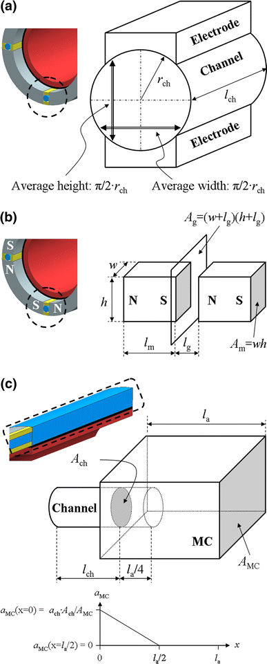

  

  Close-ups of Fig. 1: a explanation of “average height” and “average width” used to compute the output electric power; b correction for fringing at air gap between two magnets: the air gap area A _g is corrected by adding the gap length l _g to each dimension [15]; c fluid flow in MC approximated by average inertial and viscous forces: a _ch and a _MC denote the average acceleration of the fluid in the channel and the MC, respectively. It is assumed that a _MC equals a _ch times the ratio of the channel cross section A _ch to the MC cross section A _MC at the MC outlet (x = 0) and reaches zero at x = l _a/2. This corresponds to extending l _ch by a factor of l _a/4

  $$ B(r_{\text{ch}} ,l_{\text{ch}} ) = \frac{{B_{\text{r}} }}{{{{A_{\text{g}} (r_{\text{ch}} ,l_{\text{ch}} )} \mathord{\left/ {\vphantom {{A_{\text{g}} (r_{\text{ch}} ,l_{\text{ch}} )} {A_{\text{m}} (l_{\text{ch}} ) + {{l_{\text{g}} (r_{\text{ch}} )} \mathord{\left/ {\vphantom {{l_{\text{g}} (r_{\text{ch}} )} {l_{\text{m}} (r_{\text{ch}} )}}} \right. \kern-\nulldelimiterspace} {l_{\text{m}} (r_{\text{ch}} )}}}}} \right. \kern-\nulldelimiterspace} {A_{\text{m}} (l_{\text{ch}} ) + {{l_{\text{g}} (r_{\text{ch}} )} \mathord{\left/ {\vphantom {{l_{\text{g}} (r_{\text{ch}} )} {l_{\text{m}} (r_{\text{ch}} )}}} \right. \kern-\nulldelimiterspace} {l_{\text{m}} (r_{\text{ch}} )}}}}}} $$

  (34)

• Our device uses a lever arm mechanism to accelerate the fluid flow in the channels. Thus, we expect that the flow velocity and the related pressure drop will be high in the channels but irrelevant in the MC and the BC. Based on this assumption, the fluid flow in the MC and the BC was neglected and the system was reduced to the arterial wall, the channels and the membrane. The arterial wall is virtually located at the proximal end of the channels and the membrane at the distal end. Nevertheless, we realized that this simplification would not do justice to the very important fluid mass in the MC compared to the tiny fluid mass in the channels. We, therefore, derived an additional inertial force from the average acceleration experienced by the fluid in the MC (Fig. 7c). We found that this inertial force can be modelled by extending the channels by a fixed length equalling a quarter of the MC length (i.e., l _a/4). We decided to also consider the viscous force arising from this extended channel length.

• Neither the magnetic induction B, the induced electric field E _ind nor the electric current density J are constant over the channel’s cross section (B is location dependent between two magnetic poles, E _ind is a function of the flow velocity and J depends on E _ind and on the electrode geometry). We easily conclude that the Lorentz force’s magnitude is not uniform over the channel’s cross section. Thus, in the presence of MHD, the fluid flow in the channels is not axisymmetric. For simplicity, we nevertheless assumed an axisymmetric flow profile in our models.

• Based on the work of Fargie and Martin [6], we can deduce that the entry region, in which the laminar flow develops, spans the whole channels at peak forward and peak backward flow. Nevertheless, we neglect this effect and assume translational symmetry in the channels. Similar simplifications are often applied in cardiovascular engineering due to the complexity of the arterial tree with its many branchings.

Appendix 3

The solution to (12) is the sum of a homogeneous and inhomogeneous part:

$$ p_{\text{d}} (t) = k \cdot p_{{{\text{d}}\_{\text{h}}}} (t) + p_{{{\text{d}}\_\text{i}}} (t) $$

(35)

$$ p_{{{\text{d}}\_{\text{h}}}} (t) = e^{{ - \frac{{K_{\text{aw}} + K_{\text{me}} }}{R} \cdot t}} $$

(36)

$$ \begin{aligned} p_{{{\text{d}}\_\text{i}}} (t) & = \left[ {{{K_{\text{me}} } \mathord{\left/ {\vphantom {{K_{\text{me}} } {\left( {K_{\text{aw}} + K_{\text{me}} } \right)}}} \right. \kern-\nulldelimiterspace} {\left( {K_{\text{aw}} + K_{\text{me}} } \right)}}} \right] \cdot C + \sum\limits_{n = 1}^{12} {\left( {a_{n{\text{a}}} \cos (\omega_{n} t) + a_{n{\text{b}}} \sin (\omega_{n} t)} \right)} \\ & \quad + \sum\limits_{n = 1}^{12} {\left( {b_{n{\text{a}}} \cos (\omega_{n} t) + b_{n{\text{b}}} \sin (\omega_{n} t)} \right)} \\ \end{aligned} $$

(37)

where

$$ \begin{aligned} {a_{{n{\text{a}}}} = \frac{{A_{n} K_{\text{me}} \left( {K_{\text{aw}} + K_{\text{me}} } \right)}}{{\left( {K_{\text{aw}} + K_{\text{me}} } \right)^{2} + R^{2} \omega_{n}^{2} }},\quad } & {a_{{n{\text{b}}}} = \frac{{A_{n} K_{\text{me}} R\omega_{n} }}{{\left( {K_{\text{aw}} + K_{\text{me}} } \right)^{2} + R^{2} \omega_{n}^{2} }}} \\ {b_{{n{\text{a}}}} = \frac{{ - B_{n} K_{\text{me}} R\omega_{n} }}{{\left( {K_{\text{aw}} + K_{\text{me}} } \right)^{2} + R^{2} \omega_{n}^{2} }},\quad } & {b_{{n{\text{b}}}} = \frac{{B_{n} K_{\text{me}} \left( {K_{\text{aw}} + K_{\text{me}} } \right)}}{{\left( {K_{\text{aw}} + K_{\text{me}} } \right)^{2} + R^{2} \omega_{n}^{2} }}} \\ \end{aligned} $$

(38)

The coefficient k is obtained from the initial condition p _d(t = 0) = 0:

$$ k = - {{p_{{{\text{d}}\_{\text{i}}}} (0)} \mathord{\left/ {\vphantom {{p_{{{\text{d}}\_i}} (0)} {p_{{{\text{d}}\_{\text{h}}}} (0)}}} \right. \kern-\nulldelimiterspace} {p_{{{\text{d}}\_{\text{h}}}} (0)}} = - p_{{{\text{d}}\_{\text{i}}}} (0) $$

(39)

Appendix 4

Solving the homogeneous and inhomogeneous part of equation (13), one obtains:

$$ s(t) = s_{\text{h}} (t) + s_{\text{i}} (t) $$

(40)

$$ s_{\text{h}} (t) = e^{{ - \frac{b}{2a} \cdot t}} \cdot \left( {k_{1} \cos (\omega_{\text{res}} t) + k_{2} \sin (\omega_{\text{res}} t)} \right) $$

(41)

$$ \begin{aligned} s_{\text{i}} (t) & = \left( {{{\pi r_{\text{ch}}^{2} } \mathord{\left/ {\vphantom {{\pi r_{\text{ch}}^{2} } c}} \right. \kern-\nulldelimiterspace} c}} \right) \cdot C + \sum\limits_{n = 1}^{12} {\left( {a_{{n{\text{a}}}} \cos (\omega_{n} t) + a_{{n{\text{b}}}} \sin (\omega_{n} t)} \right)} \\ & \quad + \sum\limits_{n = 1}^{12} {\left( {b_{{n{\text{a}}}} \cos (\omega_{n} t) + b_{{n{\text{b}}}} \sin (\omega_{n} t)} \right)} \\ \end{aligned} $$

(42)

where

$$ \begin{gathered} \begin{array}{*{20}c} {a_{{n{\text{a}}}} = \frac{{A_{n} \pi r_{\text{ch}}^{2} \left( {c - a\omega_{n}^{2} } \right)}}{\psi },} & {a_{{n{\text{b}}}} = \frac{{A_{n} \pi r_{\text{ch}}^{2} b\omega_{n} }}{\psi },} & {b_{{n{\text{a}}}} = \frac{{ - B_{n} \pi r_{\text{ch}}^{2} b\omega_{n} }}{\psi },} & {b_{{n{\text{b}}}} = \frac{{B_{n} \pi r_{\text{ch}}^{2} \left( {c - a\omega_{n}^{2} } \right)}}{\psi }} \\ \end{array} \\ \psi = c^{2} + b^{2} \omega_{n}^{2} - 2ac\omega_{n}^{2} + a^{2} \omega_{n}^{4} \\ \end{gathered} $$

(43)

The coefficients k ₁ and k ₂ are obtained from the initial conditions s(t = 0) = 0 and s′(t = 0) = 0:

$$ \begin{array}{*{20}c} {k_{1} = - s_{\text{i}} (0),} & {k_{2} = \left( {{{k_{1} } \mathord{\left/ {\vphantom {{k_{1} } {\omega_{\text{res}} }}} \right. \kern-\nulldelimiterspace} {\omega_{\text{res}} }}} \right) \cdot {b \mathord{\left/ {\vphantom {b {\left( {2a} \right)}}} \right. \kern-\nulldelimiterspace} {\left( {2a} \right)}} - {{s_{\text{i}}^{\prime } (0)} \mathord{\left/ {\vphantom {{s_{i}^{\prime } (0)} {\omega_{\text{res}} }}} \right. \kern-\nulldelimiterspace} {\omega_{\text{res}} }}} \\ \end{array} $$

(44)

References

Armentano R, Megnien JL, Simon A, Bellenfant F, Barra J, Levenson J (1995) Effects of hypertension on viscoelasticity of carotid and femoral arteries in humans. Hypertension 26:48–54
Avolio AP (1980) Multi-branched model of the human arterial system. Med Biol Eng Comput 18:709–718
Bergel DH (1960) The static elastic properties of the arterial wall. J Physiol 156:445–457
Bergel DH (1960) The dynamic elastic properties of the arterial wall. J Physiol 156:458–469
Branover H (1978) Magnetohydrodynamic Flow in Ducts. Israel Universities Press, Jerusalem
Fargie D, Martin BW (1971) Developing laminar flow in a pipe of circular cross-section. Proc R Soc Lond A 321:461–476
Fung YC (1997) Biomechanics: circulation, 2nd edn. Springer, New York
Goto H, Sugiura T, Harada Y, Kazui T (1999) Feasibility of using the automatic generating system for quartz watches as a leadless pacemaker power source. Med Biol Eng Comput 37:377–380
Hodis A, Zamir M (2009) Arterial wall tethering as a distant boundary condition. Phys Rev E 80:051913
Horejs D, Gilbert PM, Burstein S, Vogelzang RL (1988) Normal aortoiliac diameters by CT. J Comput Assisted Tomogr 12:602–603
Jia D, Liu J, Zhou Y (2009) Harvesting human kinematical energy based on liquid metal magnetohydrodynamics. Phys Lett A 373:1305–1309
Kuecherer HF, Just A, Kirchheim H (2000) Evaluation of aortic compliance in humans. Am J Physiol Heart Circ Physiol 278:H11411–H11413
Lees C, Vincent JF, Hillerton JE (1991) Poisson’s ratio in skin. Biomed Mater Eng 1:19–23
Levy MN, Pappano AJ (2007) Cardiovascular physiology, 9th edn. Mosby Elsevier, Philadelphia
Matsch LW (1964) Capacitors, magnetic circuits, and transformers. Prentice-Hall, Englewood Cliffs
McVeigh GE, Bratteli CW, Morgan DJ, Alinder CM, Glasser SP, Finkelstein SM, Cohn JN (1999) Age-related abnormalities in arterial compliance identified by pressure pulse contour analysis: aging and arterial compliance. Hypertension 33:1392–1398
Messerle HK (1995) Magneto-hydro-dynamic electrical power generation. Wiley, Chichester
Mohiaddin RH, Underwood SR, Bogren HG, Firmin DN, Klipstein RH, Rees RS, Longmore DB (1989) Regional aortic compliance studied by magnetic resonance imaging: the effects of age, training, and coronary artery disease. Br Heart J 62:90–96
Murgo JP, Westerhof N, Giolma JP, Altobelli SA (1980) Aortic input impedance in normal man: relationship to pressure wave forms. Circulation 62:105–116
Nicoud F (2002) Hemodynamic changes induced by stenting in elastic arteries. Center for turbulence research, Annual Research Briefs, pp 335–347
Obrist D (2008) Fluidmechanics of semicircular canals—revisited. Z Angew Math Phys 59:475–497
Pfenniger A, Koch VM, Vogel R (2011) Human energy harvesting by intravascular turbine generators. In: Proceedings of the 6th international conference on microtechnologies in medicine and biology (MMB 2011), Lucerne, pp 82–83
Pfenniger A, Wickramarathna LN, Vogel R, Koch VM (2013) Design and realization of an energy harvester using pulsating arterial pressure. Med Eng Phys. doi:10.1016/j.medengphy.2013.01.001
Potkay JA, Brooks K (2008) An arterial cuff energy scavenger for implanted microsystems. In: The 2nd international conference on bioinformatics and biomedical engineering (ICBBE 2008), pp 1580–1583
Ramsay MJ, Clark WW (2001) Piezoelectric energy harvesting for bio MEMS applications. Proc SPIE 4332:429–438
Rezakhaniha R, Fonck E, Genoud C, Stergiopulos N (2011) Role of elastin anisotropy in structural strain energy functions of arterial tissue. Biomech Model Mechanobiol 10:599–611
Roberts P, Stanley G, Morgan JM (2008) Abstract 2165: harvesting the energy of cardiac motion to power a pacemaker. Circulation 118:679–680
Shau YW, Wang CL, Shieh JY, Hsu TC (1999) Noninvasive assessment of the viscoelasticity of peripheral arteries. Ultrasound Med Biol 25:1377–1388
Shercliff JA (1962) The theory of electromagnetic flow-measurement. Cambridge University Press, Cambridge
Snarski SR, Kasper RG, Bruon AB (2004) Device for electro-magnetohydrodynamic (EMHD) energy harvesting. Proc SPIE 5417:147–161
Sohn JW, Choi SB, Lee DY (2005) An investigation on piezoelectric energy harvesting for MEMS power sources. Proc IMechE Part C J Mech Eng Sci 219(4):429–436
Sutera SP, Skalak R (1993) The history of Poiseuille’s law. Annu Rev Fluid Mech 25:1–19
Tandon N, Cannizzaro C, Chao PH, Maidhof R, Marsano A, Au HT, Radisic M, Vunjak-Novakovic G (2009) Electrical stimulation systems for cardiac tissue engineering. Nat Protoc 4:155–173
Tashiro R, Kabei N, Katayama K, Tsuboi F, Tsuchiya K (2002) Development of an electrostatic generator for a cardiac pacemaker that harnesses the ventricular wall motion. J Artif Org 5:239–245
Tortoreillo A, Pedrizzetti G (2004) Flow-tissue interaction with compliance mismatch in a model stented artery. J Biomech 37:1–11
Van Buskirk WC, Watts RG, Liu YK (1976) The fluid mechanics of the semicircular canals. J Fluid Mech 78:87–98
Vasava P, Jalali P, Dabagh M (2009). Pulsatile blood flow simulations in aortic arch: effects of blood pressure and the geometry of arch on wall shear stress. In: Proceedings of the 4th European conference of the international federation for medical and biological engineering (IFMBE 2009), vol. 22, pp 1926–1929
Visser KR (1992) Electric conductivity of stationary and flowing human blood at low frequencies. Med Biol Eng Comput 30:636–640
Warriner RK, Johnston KW, Cobbold RS (2008) A viscoelastic model of arterial wall motion in pulsatile flow: implications for Doppler ultrasound clutter assessment. Physiol Meas 29:157–159
Westerhofy N, Noordergraaf A (1970) Arterial viscoelasticity: a generalized model. J Biomech 3:357–379
Westerhof N, Stergiopulos N, Noble MI (2005) Snapshots of hemodynamics: an aid for clinical research and graduate education. Springer Science + Business Media, Boston
Womersley JR (1955) Method for the calculation of velocity, rate of flow and viscous drag in arteries when the pressure gradient is known. J Physiol 127:553–563
Wong LS, Hossain S, Ta A, Edvinsson J, Rivas DH, Nääs H (2004) A very low-power CMOS mixed-signal IC for implantable pacemaker applications. IEEE J Solid-St Circ 39:2446–2456
Zurbuchen A, Pfenniger A, Stahel A, Stoeck CT, Vandenberghe S, Koch VM, Vogel R (2013) Energy harvesting from the beating heart by a mass imbalance oscillation generator. Ann Biomed Eng 44(1):131–141
Author information
Authors and Affiliations
Corresponding author