
Abstract
As societies are increasingly concerned with risks, it is important to evaluate risks not only from an individual but also from a societal perspective. Two essential dimensions of public or social risks are the inequality concerning the distribution of risks over various groups and members of society and the level of risk faced by individuals and by the society as a whole. This paper disentangles these two essential dimensions and studies people’s preferences concerning different types of allocations of risks over groups of people. We do so in a laboratory experiment with real incentives, where subjects are placed in the role of a social planner and choose between different types of allocations of risks over 10 other participants. The allocations differ only in terms of dispersion, i.e. they differ only in terms of inequality and risk. The majority of our subjects exhibit clear preferences over different types of allocations consistent with ex ante inequality and individual risk aversion, and ex post inequality and collective risk seeking behavior. These results are consistent with the literature on public risk and can be reconciled with responsibility aversion.
1 Introduction
Societies are increasingly concerned with public risks such as health epidemics, acts of terrorism, and financial crises (Quiggin 2007). One reason for this increased preoccupation is that these risks are likely to affect many members of society at the same time. Public risks entail not only individual risks for each member of society, but also risks concerning the inequalities between members of society. It is therefore important to evaluate the allocation of such risks not only from an individual, but also from a broader societal perspective.
Two essential dimensions of public risks are the inequality concerning the distribution of risks over various groups and members of society and the level of risk faced by individuals and by the society as a whole. For policymakers who design policies to cope with public risks, it is crucial to understand what role these two dimensions play in people’s evaluations of such risks. This paper studies people’s preferences concerning different types of allocations of risks over groups of people and disentangles these two essential dimensions. We do so in a laboratory experiment with real incentives.
To rule out selfish and strategic motives, we study choices between allocations of risk that cannot affect the payoffs or risks faced by the decision maker himself. Thus, we consider decision makers who can be viewed as social planners, or impartial spectators (Smith 1759). As Konow (2009) states, studying preferences of impartial spectators is particularly relevant for social choice theory, welfare analysis, and public policy, as such preferences are characterized by unbiasedness. The perspective of an impartial spectator is also relevant in other situations where people make decisions on behalf of others. One can think of parents deciding on behalf of their kids, medical doctors deciding on behalf of their patients, or managers deciding on behalf of their employees.
This study is complementary to the studies on interactions between social preferences and risks where the decision maker is affected by his decisions. Examples of such studies are the ones analyzing peer effects on risk taking and risk sharing (Rohde and Rohde2011; Linde and Sonnemans2012; Lahno and Serra-Garcia2015; Cettolin and Tausch2015) and the ones on risky dictator games (e.g. Brock et al.2013; Krawczyk and Le Lec2010) and strategic games like in Bolton et al. (2005). The decision situations we consider can be viewed as a special class of risky dictator games with 11 players where the decision maker can choose between two distributions of risks that do not differ in his own payoff. Several other experimental studies with real incentives took a similar approach in riskfree settings in order to focus on pure distributional preferences and to exclude selfish and strategic concerns (Charness and Rabin2002; Engelmann and Strobel2004; Cappelen et al.2013).
When evaluating allocations of risk across society, two notions of inequality are critical (Diamond1967; Harsanyi1955): ex-ante inequality, which concerns the procedure that generates the allocations, and ex-post inequality, which concerns the eventual allocation of outcomes (Fleurbaey2010; Sarin1985; Trautmann2009). The literature on public risk (Fishburn and Sarin1991; Keeney1980a, (Keeney 1980b); Keeney and Winkler1985; Sarin1985; Gajdos et al.2010) indicates that, next to inequalities and individual risks, the possible aggregate payoffs of the group or society also play a role in decisions to allocate risks over society. Therefore, we consider two levels of risk: individual risk and collective risk. Individual risk refers to the dispersion of the possible outcomes for one individual, irrespective of the outcomes of others. Collective risk refers to the dispersion of the total sum of outcomes. We will consider allocations of risk which differ only in terms of these inequalities and risks.
The relevance and implications of our four inequality and risk concepts can be illustrated with the following example. Consider a group of individuals and the following two possible allocations of risk. In allocation A each individual receives an independent lottery yielding €20 with 50% probability and nothing otherwise. In allocation B 50% of the individuals receive €20 and the others nothing, where the 50% fortunate ones are predetermined by a certain characteristic of the individuals, such as age. Which allocation would be considered to be socially superior? Should we give everyone an equal opportunity or should we favor particular groups in society? Allocation A, which is in line with the notion of equality of opportunity, could be regarded as superior as all individuals face equal chances. From the perspective of solidarity, though, one might argue that it is favorable to support the weakest in society such as children and the elderly, which will lead to predetermined allocations, as is the case in allocation B. This conflict between equality of opportunity and solidarity is present in many real life situations such as the allocation of donor organs, student placement procedures, the allocation of power plants, and the design of rescue plans in case of calamities.
Now suppose that allocation B is replaced by allocation C, where with a 50% probability all individuals receive €20 and otherwise all individuals receive nothing. This allocation C guarantees that everyone receives the same outcome but does not take away the uncertainty whether this outcome will be high or not. Whether or not a person finds allocations A and C different from each other depends partly on the order in which he processes risks and inequalities. A person who first processes risk and then inequality may argue that in both allocation procedures all individuals get the same lottery and thereby have the same chances, i.e. equal opportunities, so that there is no inequality. This person will find both procedures equivalent. A person who first processes inequalities and then risk may argue that in allocation C there will always be equality after resolution of the uncertainty, whereas in allocation A it is very likely that there will be inequality after resolution of uncertainty. This person will not find the two procedures equivalent. Thus, the order in which the two types of dispersion, inequality and risk, are processed affects preferences and, thereby, also sheds light on people’s concerns for procedural fairness.
The aim of this paper is twofold. The first aim is to analyze people’s preferences over allocations of risks over groups of people. The second aim is to disentangle these preferences into concerns for risk and inequality. During the experiment, subjects are placed in the role of a social planner and choose between different types of allocations of risks over 10 other participants. The allocations differ only in terms of dispersion, i.e. they differ only in terms of inequality and risk. If subjects care only about the expected payoffs of individuals and the expected aggregate payoff in the group, they will be indifferent between these allocations. Yet, if they also care about risk and inequality, they will not be indifferent.
Though many studies have analyzed people’s concerns for risk, and many have analyzed people’s concerns for inequality, only very few have studied how concerns for risk and inequality are integrated (Bolton et al.2005; Kroll and Davidovitz2003; Keller and Sarin1988; Bian and Keller1999; Loomes1982). This paper is the first to experimentally, and by using real incentives, analyze people’s preferences over public risks which affect other people. Our experiment is inspired by a previous study (Rohde and Rohde 2011) which found that subjects had a strong preference for an allocation rule which gave every individual the same independent risk, while subjects were reluctant to implement allocation rules which favored a randomly selected, predetermined number of individuals. The experiment in the current paper was designed to provide insights into the reasons for this preference.
The results of our experiment are striking. We observe a clear pattern in individuals’ preferences over different allocation procedures. Subjects are not indifferent between these procedures and take risks and inequalities into account. In particular, our subjects cannot be viewed as social planners who maximize utilitarian social welfare functions of selfish individual expected utilities. Moreover, we find that our subjects are averse towards ex ante inequality and individual risk, while they seek ex post inequality and collective risk. Though surprising at first sight, we will show that these results do not contradict the existing literature.
2 Public risk: Inequality and risk
The types of risk allocations we consider in this paper differ in terms of ex ante inequality, ex post inequality, individual risk, and collective risk. While these concepts are different, they are closely related. Before giving exact definitions, we will consider two examples that clearly illustrate the differences and similarities between the inequality and risk concepts. The first example is from Diamond (1967). Consider two people: Ann and Bob. We flip a coin to determine their utility allocations. In the first procedure (Procedure I) Ann will get one unit of utility and Bob zero, irrespective of the outcome of the coin flip. In the second procedure (Procedure II) Ann gets one unit of utility, and Bob zero, in case of Heads, and the utilities are reversed in case of Tails. Table 1 summarizes these utility levels.
A social planner merely concerned about ex post inequality would argue that in both procedures one person would end up with one unit of utility and the other with zero units of utility, irrespective of the outcome of the coin flip. Thus, he would be indifferent between both procedures. A social planner who was concerned about ex ante inequality would argue that in Procedure I there is inequality in terms of expected utilities,Footnote 1 whereas in Procedure II there is no such inequality. He would then favor Procedure II. This illustrates the difference between ex ante and ex post inequality.
In both Procedures I and II the total utility is always one unit. Both procedures, therefore, impose zero collective risk. Yet they do differ in terms of individual risk in the sense that Procedure I generates no individual risk, i.e. risk from the perspective of a single individual other than the social planner, whereas Procedure II does. If the social planner were individual risk seeking, then he would favor Procedure II in terms of individual risk, which together with ex ante inequality aversion would make him choose Procedure II, as ex post inequality and collective risk are the same in both procedures. If, however, he were individual risk averse, then he would favor Procedure I in terms of individual risk, while he favors Procedure II in terms of ex ante inequality, making it impossible for us to predict what he will choose. This example shows that it is sometimes impossible to disentangle attitudes towards individual risk and ex ante inequality.
To illustrate the difference between individual and collective risk and their relation to ex ante and ex post inequality, let’s consider a third procedure: Procedure III. This procedure differs from the other two in the sense that the utilities of Ann and Bob will be determined independently of each other. More precisely, the coin will be flipped twice: once for Ann and once for Bob. Heads yields a utility level of one and Tails zero. The payoffs are given in Table 1. The social planner is asked to choose between Procedures II and III. Note that the individual risk in both procedures is the same: one unit of utility with 50% probability and zero otherwise. Thus, a social planner merely concerned about individual risk would be indifferent between the two procedures. In terms of total payoff, though, Procedure III is riskier. Thus, Procedure III generates more collective risk. A collective risk averse social planner would then favor Procedure II.
Procedures II and III do not differ in terms of ex ante inequality as both procedures yield the same expected utilities.Footnote 2 Yet they do differ in terms of ex post inequality. Unlike Procedure II, Procedure III offers a 50% probability of zero inequality ex post. If the social planner were ex post inequality seeking, then he would favor Procedure II, in line with collective risk aversion. If, instead, he were ex post inequality averse, then he would favor Procedure III, which would counteract collective risk aversion. Thus, it is sometimes impossible to disentangle attitudes towards collective risk and ex post inequality.
These examples contain two messages. First, they show the distinction between the two inequality concepts and between the two risk concepts. Second, they show that while inequality and risk are different, they are not completely independent from each other. Our experiment will allow us to disentangle attitudes towards risk and inequality by considering choices that circumvent the interdependence between the four concepts. Before presenting the experimental design in Sections 3 and 4, the rest of this section will give exact definitions of the risks and inequalities we will consider.
We consider a setting with n+1individuals 0,…,n. Individual 0 is the social planner whose preferences we are interested in. The social planner chooses between allocations of risk for the n other players. His own payoff is unaffected by his decisions. Our setting thereby resembles a public risk setting (Keeney1980a, (Keeney 1980b)) with the crucial difference being that the outcomes we consider are continuous monetary payoffs instead of binary outcomes such as life or death.
Inequality and risk are dispersions of outcomes over individuals and states of nature. We will operationalize the inequality and risk concepts by measuring the corresponding dispersions through standard deviations. The non-parametric results of this paper are unaffected by this choice of measure for dispersion: different measures could be used as long as the ordering of the allocations in the experiment according to each individual risk or inequality concept would be unaffected. The parametric results could, in theory, be affected by the particular choice for dispersion-measure. Yet, using other commonly used measures for inequality such as the Gini index and the Theil index did not affect the parametric results qualitatively, except for the significance level of gender effects and of ex ante inequality aversion. Therefore, we only report the results based on standard deviations in the main text and report the Gini and Theil results in Online Appendix A.
An ex post allocation x = (x 1,…,x n ) yields outcome \(x_{i} \in \mathbb {R} \) to individual i and thereby specifies a payoff to all individuals except for the decision maker whose payoff is always unaffected. An ex ante allocation L = (p 1:x 1,…,p m :x m ) for any finite m yields ex post allocation x j with probability p j for j=1,…,m. An ex post allocation is an allocation that results after risk is resolved. An ex ante allocation is a lottery of ex post allocations and thereby describes the probabilities that particular ex post allocations may result. By x i,j we denote the outcome for individual i in ex post allocation x j .
The individual expected value of individual i in ex ante allocation L = (p 1:x 1,…,p m :x m ) is defined by \(IEV_{i}(\mathbf {L}) = {\sum }_{j=1}^{m} p_{j} x_{i,j}.\) The average expected value of ex ante allocation L is then given by \(\overline {IEV}(\mathbf {L}) = {\sum }_{i=1}^{n} \frac {1}{n} IEV_{i}(\mathbf {L}).\) We define ex ante inequality as the standard deviation of the distribution of individual expected values: \(EAI(\mathbf {L}) = \sqrt {{\sum }_{i=1}^{n} \frac {1}{n} \left (IEV_{i}(\mathbf {L}) - \overline {IEV}(\mathbf {L}) \right )^{2}}.\) A decision maker who is merely concerned about ex ante inequality behaves as if he first processes the risk dimension (IEV) and then the interpersonal dimension of an ex ante allocation.
The ex post average payoff of ex post allocation x = (x 1,…,x n ) is given by \(\boldsymbol {\bar {x}} = {\sum }_{i=1}^{n} \frac {1}{n} x_{i}.\) The ex post inequality of ex post allocation x = (x 1,…,x n ) is the standard deviation of the ex post distribution and is given by \(EPI(\mathbf {x}) = \sqrt {{\sum }_{i=1}^{n} \frac {1}{n} \left (x_{i} - \boldsymbol {\bar {x}}\right )^{2}}.\) The expected ex post inequality of ex ante allocation L = (p 1:x 1,…,p m :x m ) is given by \(EEPI(\mathbf {x}) = {\sum }_{j=1}^{m} \left (p_{j} EPI(\mathbf {x}_{j})\right ).\) A decision maker who is merely concerned about expected ex post inequality behaves as if he first processes the interpersonal dimension (EPI) and then the risk dimension of an ex ante allocation.
In line with the literature on public risk, we also consider two types of risk: individual risk and collective risk. The individual risk of individual i in ex ante allocation L = (p 1:x 1,…,p m :x m ) is defined by \(IR_{i}(\mathbf {L}) = \sqrt {{\sum }_{j=1}^{m} p_{j} \left (x_{i,j} - IEV_{i}(\mathbf {L}) \right )^{2}}.\) We define collective risk as the standard deviation of the total payoff that accrues to the group of individuals 1,…n. The collective expected value of ex ante allocation L = (p 1:x 1,…,p m :x m ) is defined by \(CEV(\mathbf {L}) = {\sum }_{j=1}^{m} p_{j} \left ({\sum }_{i=1}^{n} x_{i,j}\right ).\) The collective risk of ex ante allocation L = (p 1:x 1,…,p m :x m ) is defined by \(CR(\mathbf {L}) = \sqrt {{\sum }_{j=1}^{m} p_{j} \left (\left ({\sum }_{i=1}^{n} x_{i,j}\right ) - CEV(\mathbf {L}) \right )^{2}}.\)
We will say that the social planner is ex ante inequality averse (seeking) if he strictly prefers ex ante allocations with lower (higher) ex ante inequality, everything else held constant. We will say that he is ex ante inequality neutral if ex ante inequality does not play any role in his preferences. Aversion, neutrality, and seeking are defined in a similar way for expected ex post inequality, individual risk, and collective risk.
3 Allocation types
In our experiment subjects make pairwise choices between different types of risk allocations, which allows us to disentangle attitudes towards risks and inequalities. We let n equal 10 so that there are 11 participants per session (10 + the decision maker). Let (50%:10,50%:5) denote a Basic Lottery that yields €10 with 50% probability and €5 otherwise. From such a basic lottery we derive five allocation types. To enhance readability, the phrases ‘all individuals’ and ‘all subjects’ will from now on refer to all individuals except the decision maker. The different allocation types are as follows:
-
Independent Lottery (50% : 10, 50% : 5) All individuals independently receive the lottery (50% : 10, 50% : 5), i.e. this lottery is resolved 10 times.
-
Common Lottery (50% : 10, 50% : 5) The lottery (50% : 10, 50% : 5) is resolved once and all 10 individuals receive the same outcome of the lottery.
-
Random Distribution (5:10, 5:5) Half (50%) of the 10 individuals are randomly selected and receive €10 while the others receive €5. All individuals have equal probability of being selected to receive the larger outcome.
-
IDbased Distribution (5:10, 5:5) Half (50%) of the 10 individuals are selected based on their identity (details follow in Section 4) and receive €10 while the others receive €5.
-
Common Outcome (10:7.5) All individuals receive €7.50.
If all 10 individuals affected by the choices have self-regarding preferences in the sense that they derive utility only from their own payoffs and probabilities, then they are indifferent between all allocation types except the common outcome. A social planner with a utilitarian welfare function would then also be indifferent between these allocation types. Our experiment allows us to test for this. Deviations from indifference will suggest that the social planners are not using a utilitarian welfare function with individual self-regarding utilities as input.
Table 2a summarizes the five allocation types in terms of the degrees of risks and inequalities as defined in the previous section. Pairwise comparisons between these lotteries allow us to disentangle concerns for risks and inequalities. Consider, for instance, the choice between a Random Distribution and the corresponding IDbased Distribution. These allocations differ in only one respect: in the Random Distribution the social planner does not know up front who will receive which outcome, while in the IDbased Distribution the social planner does. Thus, the IDbased Distribution imposes a larger ex ante inequality than the Random Distribution, but the same expected ex post inequality and risks. A preference between these allocations therefore directly reveals the attitude towards ex ante inequality.
The Random Distribution differs from the corresponding Common Lottery in two respects: the Random Distribution imposes a larger expected ex post inequality, whereas the Common Lottery imposes a larger collective risk. Therefore, a preference between these two allocations gives information about the attitudes towards ex post inequality and collective risk. If, for instance, a person is collective risk averse and prefers the Common Lottery to the Random Distribution then he must be expected ex post inequality averse. A preference between the Random Distribution and the corresponding Independent Lottery similarly reveals attitudes towards ex post inequality and collective risk. The Common Outcome then allows us to reveal the attitude towards individual risk.
4 Experimental design
In the experiment we consider three basic lotteries: (50% : 10, 50% : 5), (20% : 11.5, 80% : 6.5), and (30% : 4, 70% : 9), where the outcomes are in Euros. This paper investigates preferences of social planners. We therefore want to keep the salience of the payoffs of the decision makers themselves as low as possible. To this end we ensure that their payoffs don’t depend on their decisions nor on the questions they face.Footnote 3 Thus, we keep the payoffs of the decision makers and the corresponding expected payoffs for the other 10 subjects constant throughout the experiment. We fix this payoff at €7.5, the expected value of the basic lotteries. Therefore, preferences cannot be driven by differences in individual expected values. We also keep the absolute difference between the highest and the lowest outcome constant throughout the experiment (equal to €5). We do so to prevent subjects from using the heuristic to base their decisions merely on the difference between the highest and lowest outcomes without paying attention to the probabilities. The lotteries differ in the relative chances of obtaining the high outcome. In lottery (20% : 11.5, 80% : 6.5) the chance of receiving the high outcome is relatively low, whereas in lottery (30% : 4, 70% : 9) this chance is relatively high.
For each of the three basic lotteries we derive the five different allocation types as described in the previous section. Subjects make pairwise choices between these allocations, resulting in 3 times 10 binary choices as summarized in Table 3. Thus, the choices subjects make are choices between allocation types that are based on the same basic lottery. We repeat these choices for different basic lotteries.
For each of the three basic lotteries and for each allocation type, Table 2 gives the values of the risks and inequalities. In the IDbased Distribution subjects are selected based on their student ID number.Footnote 4 At the start of the experiment all subjects have to give their student ID number to the experimenter. The experimenter takes the sum of all digits in each student’s ID number and the ones with the lowest sums receive the highest outcomes. In case of two students having the same sum of digits, the lower student ID number yields the higher outcome. For individual risk in the IDbased Distribution we assume that the social planner imagines himself in the position of the individuals, who do not know the sum of digits of the student ID numbers of the other participants. For ex ante inequality the social planner takes into account the fact that the ones with a high payoff are predetermined by personal characteristics.
At the end of the session we randomly chose one of the subjects to be the social planner and randomly chose one of his questions to determine what the payoff of every subject would be. In addition to these earnings all subjects receive €5.00 for participating.
4.1 Subjects, payment, and procedures
We recruited 55 undergraduate students from Erasmus University Rotterdam (34 male, 21 female, 52 economics students) for 5 sessions of 11 subjects. All participants were recruited using ORSEE (Greiner 2004). Each subject participated in only one session. To ensure anonymity and avoid any communication during the experiment, subjects were seated in sight-shielded cubicles. After being seated, subjects received written instructions, which they could study at their own pace. They could ask questions privately in case they needed clarification. The experiment did not start before all subjects had correctly answered a series of comprehension questions. The instructions and comprehension questions are in Online Appendix C.
The experiment was computerized using Z-tree (Fischbacher 2007). Every question was displayed in a different screen, where one option was shown on the left-hand side and the other on the right-hand side. We randomized the order of the questions and the left/right position of the options. The experiment started with three practice questions, where each of the five allocation types was an option at least once. The allocation types in these practice questions were based on different basic lotteries than the other questions of the experiment. At the end of the experiment subjects were paid anonymously.
5 Results
The results of our experiment are analyzed in two stages. In the first stage we make use of non-parametric tests. In the second stage we employ logit regressions to further analyze the data. All tests reported in this section are two-sided, unless stated differently.
5.1 Preferences over allocation types
Table 3 (fourth column) shows, for each question, the percentage of subjects choosing Option A. This table thereby reveals the options that would be chosen under majority voting by a team of social planners: the options that are preferred by more than 50% of the subjects. If choices were completely random then the percentage of subjects choosing Option A would be 50%, as the order in which the options are presented is randomized. The last column of the table gives the two-sided p-values of binomial tests with assumed probability 50%. For each question a separate binomial test was done. We repeated these binomial tests for data pooled by question type, independently of the basic lottery, as summarized in Table 4. For instance, we combined all choices between independent lotteries and random distributions, no matter which underlying basic lottery, i.e. we combined questions 1, 11, and 21.
From the pooled data we conclude that, based on majority voting, subjects have the following preferences over allocation types:
where the strict preferences indicate significance at the 5% level.Footnote 5 The weak preference indicates weak significance with the common outcome weakly preferred to the common lottery with a pooled p-value of 0.119.
When looking at the data per question, we see that the independent lottery is preferred over the common lottery, but not significantly. Yet, the pooled data show a significant difference. The common outcome is significantly preferred over the common lottery only for the basic lottery (30%:4,7%:9). For the remaining questions, a few significance levels are lower than in the pooled data, but there are no strong contradictions of the abovementioned preference pattern.
To test for consistency with the abovementioned pattern within subjects, we computed the number of times a subject chose consistently with it for each question type. The results of this consistency-check are in Table 5, where we show the number of subjects who are consistent with the general pattern in 0, 1, 2, or 3 choices per question type. We see that for each question type substantially more than 50% of the subjects are consistent with the pattern in a majority of their choices (in at least 2 choices), which supports consistency within subjects. At the same time we also see that for some question types there is a substantial proportion of subjects (between 10% and 25%) who are always consistent with the opposite of the pattern for this question type, which shows that there is heterogeneity between subjects. Therefore, the results reported in this paper should be interpreted as reflecting majority preferences of a heterogeneous group of decision makers.
Table 5 illustrates the within-subject-consistency for each question type separately. For every subject we also counted the total number of choices (out of the 30 possible choices) that are in line with the general pattern described above. These counts are summarized in Fig. 1. A binomial test shows that significantly more than 50% of the subjects (37 out of 55) are consistent with this pattern in at least two-thirds of their choices (p-value = 0.003).Footnote 6
The results so far are consistent with the findings of Keller and Sarin (1988); Bian and Keller (1999), who conducted surveys asking people to choose between some of our allocation types in health and safety contexts with binary outcomes (alive or dead). Robson (1996) provides an evolutionary basis for the independent lottery being preferred over the common lottery. Kroll and Davidovitz (2003), however, found that 8-year-old children prefer a common lottery to the corresponding independent lottery. Loomes (1982) found a lot of heterogeneity between people’s preferences. Yet, Loomes (1982) and Kroll and Davidovitz (2003) considered decision makers who were included in the group of people affected by the decisions, and thereby did not rule out selfish motives. Thus, any difference between these two studies and ours may at least partly be caused by selfish motives.
5.1.1 Interpretation of the results in terms of attitudes towards inequality and risk
Our subjects are clearly not indifferent between all allocation types. The social planner with a utilitarian welfare function and individual self-regarding utilities as inputs is thereby rejected by our data.
For further interpretation of the results we assume that decision makers have consistent preferences in the sense that if they are averse (seeking or neutral) to a risk or inequality concept in one question, they are so in all questions.
The preference for the Random Distribution over the IDbased Distribution is highly significant. Looking at Table 2 we see that the only difference between these two allocation types is the ex ante inequality. Thus, we can conclude that subjects are ex ante inequality averse.
The Common Lottery and the Random Distribution differ in only two respects: Common Lottery has a higher collective risk and Random Distribution has a higher expected ex post inequality. The preference for the Common Lottery over the Random Distribution is therefore consistent with only two combinations of attitudes towards expected ex post inequality and collective risk:
-
expected ex post inequality averse & collective risk averse, neutral, or seeking
-
expected ex post inequality seeking or neutral & collective risk seeking.
The Independent Lottery differs from the Common Lottery also in two respects: the Independent Lottery has a higher expected ex post inequality and the Common Lottery has a higher collective risk. The preference for the Independent Lottery over the Common Lottery is therefore consistent with only two combinations of attitudes towards expected ex post inequality and collective risk:
-
expected ex post inequality averse or neutral & collective risk averse
-
expected ex post inequality seeking & collective risk averse, neutral, or seeking.
The Common Outcome and the Random Distribution also differ in only two respects: the Random Distribution has both a higher expected ex post inequality and a higher individual risk than the Common Outcome. From the preference for the Common Outcome over the Random Distribution we can therefore conclude that subjects cannot be both expected ex post inequality seeking and individual risk seeking. Similarly, from the preference for the Common Outcome over the Common Lottery we can conclude that subjects cannot be both individual risk seeking and collective risk seeking. Finally, from the indifference between the Independent Lottery and the Common Outcome we can conclude that people must be expected ex post inequality seeking/neutral, individual risk seeking/neutral, or collective risk seeking/neutral.
To summarize, of the 34=81 theoretically possible combinations of inequality and risk attitudes, two are consistent with the findings:
-
ex ante inequality averse - ex post inequality averse - individual risk seeking - collective risk averse
-
ex ante inequality averse - ex post inequality seeking - individual risk averse - collective risk seeking
These two patterns imply that subjects are not neutral to any of the risk and inequality concepts we consider. They therefore do not process risks and inequalities purely sequentially.
5.2 Relative importance of risk and inequality
In order to determine which of the two combinations of attitudes towards inequalities and risks is most consistent with the data, we employ a logit estimation. For every allocation type j we let ante j , post j , ind j , and coll j denote its ex ante inequality, expected ex post inequality, individual risk, and collective risk, respectively. We assume that the evaluation of an allocation type is based on a weighted sum of the (dis)utility generated by each motive, where we assume diminishing sensitivity, i.e. the value of allocation j for individual i is given byFootnote 7
where e i,j is an individual-specific error term. The probability that an individual chooses allocation j when he is offered the choice between allocation j and allocation k, is given by
We estimate the coefficients γ ante , ? post , γ ind , and γ coll , by using robust variance estimators clustered by subject. Thereby we correct for possible differences in behavior between subjects and interdependencies in choices within subjects.
Table 6 reports the estimated coefficients and their p-values. Rows 2 till 5 of the table show that all motives play a highly significant role. The coefficients show that people are ex ante inequality averse, ex post inequality seeking, individual risk averse, and collective risk seeking. One may wonder whether the high significance levels may be due to the fact that we assume the responses to different questions to be independent, whereas this independence may be violated if subjects make transitive choices. Therefore, we also ran the same regression including only the responses to questions 1, 5, 8, 10, 11, 15, 18, 20, 21, 25, 28, and 30. Qualitatively, the results of this regression are the same as for the regression with all data: same attitudes towards the motives and equally high significance levels (10%, 5%, or 1%).
To further assess the robustness of our results, we also estimated a mixture model where every individual is of one of two types, the results of which are reported in Online Appendix B. The two types of individuals may have different preferences. We expected that the two types would be consistent with patterns (I) and (II) of Section 5.1, respectively. Yet, this turned out not to be the case: with a 66% probability a subject was in line with the results of our logit estimation and otherwise he had preferences that deviate from both (I) and (II), being ex ante inequality and collective risk seeking and ex post inequality and individual risk neutral.
At first sight it is counterintuitive and thereby surprising to see that people are ex post inequality seeking and collective risk seeking. Studies on inequality in riskless contexts, for instance involving dictator and ultimatum games, suggest that people are inequality averse, which seems to contradict ex post inequality seeking. Yet there need not be a contradiction: one has to realize that in a riskless setting, ex ante and ex post inequality coincide. Therefore, in riskless contexts we cannot disentangle the two inequality concepts. Moreover, our experiment only considers inequalities generated by different distributions of risks over subjects, given an equal distribution of individual expected utilities.
One motive which possibly underlies ex post inequality and collective risk seeking is responsibility aversion (Leonhardt et al. 2011). This motive refers to a preference of people to minimize their causal role in determining final outcomes. Responsibility averse people prefer to transfer responsibility to “nature”, thereby having a tendency to like risky options where nature determines the final outcome.
By having a closer look at expected ex post inequality and collective risk our findings can be reconciled with intuition as follows. Keeney (1980a) and Ben-Porath et al. (1997) showed that collective risk seeking is closely related to ex post inequality aversion. They show that when omitting collective risk, collective risk seeking is translated into ex post inequality aversion, as we saw in the comparison between Procedures II and III in Section 2. Thus, when not properly accounting for collective risk, the usual finding of ex post inequality aversion could, theoretically, be the net result of a combination of two pure attitudes: pure ex post inequality seeking and pure collective risk seeking. In order to investigate whether this is the case for our data, we also ran logit regressions with only one motive at a time.
The results are reported in rows 6 till 9 of Table 6. There we see that if we only focus on ex ante inequality, we find significant aversion, which is in line with our previous estimation. Similarly, we find individual risk aversion if we isolate that motive. We find collective risk seeking, which is also in line with previous estimations. Yet, when only incorporating ex post inequality, we find significant ex post inequality aversion. Thus, if we do not properly account for collective risk, collective risk seeking is translated into ex post inequality aversion, resulting in a net effect of ex post inequality aversion when combined with pure ex post inequality seeking. This is an interesting result, which shows that inequality is a complex concept that should be interpreted with care. It suggests that the common ex post inequality aversion may partly be driven by concerns for collective risk. The results are in line with Engelmann and Strobel (2004) who, in a riskless setting, also found that inequality aversion was driven by other basic concerns such as maximin preferences.
Finally, we ran logit regressions including only the inequality measures (rows 10-11 of Table 6) and only the risk measures (rows 12-13 of Table 6). There we see insignificant ex post inequality aversion, in line with the above mentioned results.
Many studies on individual risk attitudes show that women are more risk averse than men (Eckel and Grossman 2008). In order to analyze whether there is a gender effect in our analysis, we repeated all logit regressions, now including the relevant variables multiplied by a dummy variable being 1 for males and 0 for females. The estimates for this regression are given in Table 7. Men and women have similar and significant attitudes towards risks and inequalities. There are differences between men and women, though, in the levels of their attitudes. Men are significantly less ex post inequality and collective risk seeking than women. Moreover, men are significantly less individual risk averse than women.
6 Discussion
This paper investigated decision makers’ preferences over distributions of risks that do not affect their own payoffs. Such decisions are made, for example, by governments allocating resources to groups in society, by health-policy makers deciding whom to vaccinate, by managers allocating resources over their employees, and by insurance companies deciding which risks to insure. Since the decision makers we consider obtain payoffs that are independent of their decisions, we call them impartial spectators, or social planners.
We made several choices when designing the experiment, in order to mimic decision situations that social planners may face in reality. First of all, we wanted to keep the salience of the payoffs of the decision makers as low as possible. To this end we fixed the payoffs of decision makers at €7.50 and only considered allocations that have an expected payoff per person equal to the payoff of the decision maker. We also referred to the payoff of the decision maker only in the instructions and did not display them further in the experiment.Footnote 8 In line with this low salience of decision makers’ own payoffs, we used inequality measures based only on the dispersion of payoffs between individuals other than the decision maker.
An interesting avenue for future research is to analyze decision situations where the payoffs of the decision makers are more salient and to employ dispersion measures that include the decision maker in the group of interest. One can also consider situations where the decision maker is always better or always worse off than every individual in the group he decides for. It will also be interesting to consider situations where the decision maker is part of the group for which he decides, either with or without a veil of ignorance. This will reveal whether and how decisions concerning public risks change when decision makers are influenced by their own decisions.
Moreover, our analysis focussed on the decisions made by social planners without analyzing the well-being of the people affected by the chosen allocations of risk. As impartial spectators may want to choose allocations of risks that maximize the well-being of the group they are deciding for, it will also be important for future studies to analyze the degree of satisfaction of this group with the allocations chosen by the impartial spectators.
We also recommend further experiments to analyze a wider variety of allocations with different basic lotteries. It will be of interest to analyze whether our results are robust to a change in the difference between the lowest and highest payoff, to a change in the expected values of the basic lotteries, and to an extension to the domain of losses. A further extension is to allow subjects to express indifference.
As mentioned before, our study is closely related to theoretical and empirical studies on public and social risk (Fishburn and Sarin1991; Keeney1980a, ??; Keeney and Winkler1985; Sarin1985; Gajdos et al.2010). These studies differ from ours in the sense that they consider two possible outcomes for individuals, whereas we consider a wider range of possible outcomes, having a continuum of possible outcomes in mind. The measures of dispersion that we use are therefore also different from theirs. An important adjustment we made is that our measures are also sensitive to the exact difference between the highest and lowest payoffs in a group of people. As we wanted our measures to depend on this difference, we also decided not to use the measures introduced by Fishburn and Sarin (1994, 1997). Fishburn and Sarin (1994, 1997) consider benefits and risks (costs) to groups of people without restricting them to be binary. Their measures of fairness take into account that higher benefits are preferred to lower ones. Yet, they are based on the number of people that a person envies and thereby do not depend on the exact difference between the highest and lowest payoffs. Future experiments, which vary the difference between the highest and lowest payoff in society, can be used to test which measures describe impartial spectators’ preferences best.
7 Conclusion
This paper analyzed social planners’ attitudes towards public risks through an experiment. Public risks entail two types of dispersions in outcomes: dispersions within individuals, risks, and dispersions between individuals, inequalities. We analyzed people’s preferences over public risks that differ only in terms of these dispersions. The experimental setup also allowed us to disentangle attitudes towards ex ante inequality, ex post inequality, individual risk, and collective risk.
In the experiment with real incentives subjects chose between allocations of risks over 10 other subjects. Subjects were impartial spectators in the sense that their decisions could not affect their own payoffs. Our main result is that subjects had clear preferences over the allocation types which differed only in terms of risk and inequality. This rules out the possibility for these social planners to maximize a utilitarian welfare function with individual self-regarding utilities as inputs.
The results also show that our subjects are ex ante inequality and individual risk averse and ex post inequality and collective risk seeking. While we expected to find ex ante inequality aversion and individual risk aversion, ex post inequality seeking and collective risk seeking were surprising at first sight. Yet, a closer look at collective risk and ex post inequality helps to understand this result. These two concepts are closely related and intuitively hard to disentangle. The literature on public risk has shown that a collective risk seeking attitude translates into an ex post inequality averse attitude when not properly accounted for. This suggests that one’s intuitive expectation of ex post inequality aversion might in fact be confounded with collective risk seeking. Responsibility aversion possibly underlies a tendency to be collective risk and ex post inequality seeking.
Our findings provide useful insights for public risk management. Think of a choice between two technologies to reduce risks—for instance two vaccines for a contagious disease. One vaccine works moderately well for everybody, reducing the risk of getting the disease partially, but equally, for everybody. The other vaccine entirely eliminates the risk of getting the disease for some people and has no effect for others. The first vaccine can be viewed as an independent lottery and the second as a random lottery. Hence, our experiment implies a preference for the first vaccine.
Though one should be careful in drawing general conclusions from single experiments, one general conclusion can be drawn from this study: decision makers who have to (re)distribute resources over groups of people will not merely pay attention to inequalities in expected outcomes, but also to inequalities in risks. In particular, they will pay attention to ex ante and ex post inequality and to individual and collective risk. Disregarding any of these criteria may lead to suboptimal decisions.
Notes
A similar reasoning holds under other models of individual decision making, like, for instance, prospect theory, as long as monotonicity holds.
A similar reasoning holds under other models of individual decision making, like, for instance, prospect theory, as long as monotonicity holds.
Our inequality measures are based on the group of ten others, excluding the decision maker. We repeated our analyses with inequality measures based on standard deviations including all 11 individuals, including the decision maker. These results were similar to the ones excluding the decision maker, with the same signs of the coefficients and same significance levels. Therefore, we do not report them.
We wanted ex ante inequality to result from the mere fact that the allocation is based on personal characteristics, while keeping these characteristics as neutral as possible so as not to arouse any additional emotions. The sum of the digits in student ID numbers have the advantage that they are relatively random and neutral characteristics of our subjects. We repeated the analyses in this paper excluding the IDbased distribution and ex ante inequality. This did not affect our results: the signs and significance levels of the coefficients in Table 6 were unaffected.
If subjects were to make their choices randomly, they would choose Option A with 50% probability in each question, as in 50% of the cases Option A was shown on the left and in the other cases on the right of the screen. Moreover, their choices would be completely independent between different questions, as the left-right position on the screen was randomized for each question independently. Thus, every p-value of the pooled data corresponds to a test of the hypothesis that subjects respond entirely randomly to one type of question. This actually is a test of the joint hypothesis that subjects choose Option A with 50% probability and that the responses to the same question type over different basic lotteries are independent.
Twenty-one of them are male and 16 female.
Fig. 1 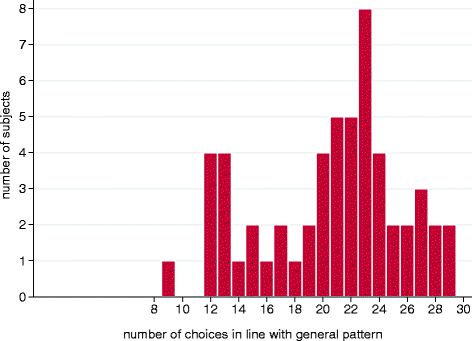
Summary of consistency with the general pattern
The natural logarithm implies diminishing sensitivity, i.e. decreasing marginal impacts of inequalities and risks. For instance, the more ex ante inequality, the less impact an increase in ex ante inequality will have. The marginal impact of each inequality or risk variable is unaffected by the levels of the other variables. We add a constant 1 to each variable before taking the natural logarithm in order to ensure that if a variable takes on a zero value, its effect on the evaluation is zero as well: ln(1+0)=0. In terms of implied choice behavior the value function we use is equivalent to the function
$$V_{i,j} = (1+ante_{j})^{\gamma_{ante}} \ (1+post_{j})^{\gamma_{post}} \ (1+ind_{j})^{\gamma_{ind}} \ (1+coll_{j})^{\gamma_{coll}} \ e^{\varepsilon_{i,j}}. $$This is an important difference between our study and the one by Engelmann and Strobel (2004).

References
Ben-Porath, E., Gilboa, I., & Schmeidler, D. (1997). On the measurement of inequality under uncertainty. Journal of Economic Theory, 75, 194–204.
Bian, W.-Q., & Keller, R.L. (1999). Chinese and Americans agree on what is fair, but disagree on what is best in societal decisions affecting health and safety risks. Risk Analysis, 19, 439–452.
Bolton, G.E., Brandts, J., & Ockenfels, A. (2005). Fair procedures: Evidence from games involving lotteries. Economic Journal, 115, 1054–1076.
Brock, J.M., Lange, A., & Ozbay, E.Y. (2013). Dictating the risk - experimental evidence on giving in risky environments. American Economic Review, 103, 415–37.
Cappelen, A.W., Konow, J., Erik, Ø.S., & Bertil, T. (2013). Just luck: An experimental study of risk taking and fairness. American Economic Review, 103, 1398–1413.
Cettolin, E., & Tausch, F. (2015). Risk taking and risk sharing: Does responsibility matter? Journal of Risk and Uncertainty, 50, 229–248.
Charness, G., & Rabin, M. (2002). Understanding social preferences with simple tests. Quarterly Journal of Economics, 117, 817–869.
Diamond, P.A. (1967). Cardinal welfare, individual ethics, and interpersonal comparison of utility: Comment. Journal of Political Economy, 75, 765–766.
Eckel, C.C., & Grossman, P.J. (2008). Men, women and risk aversion: Experimental evidence. In: C.R. Plott, V.L. Smith (Eds.), Handbook of experimental economics results (Vol. 1), Amsterdam: North-Holland.
Engelmann, D., & Strobel, M. (2004). Inequality aversion, efficiency, and maximin preferences in simple distribution experiments. American Economic Review, 94, 857–869.
Fischbacher, U. (2007). z-Tree: Zurich toolbox for ready-made economic experiments. Experimental Economics, 10, 171–178.
Fishburn, P.C., & Sarin, R.K. (1991). Dispersive equity and social risk. Management Science, 37, 751–769.
Fishburn, P.C., & Sarin, R.K. (1994). Fairness and social risk I: Unaggregated analyses. Management Science, 37, 1174–1188.
Fishburn, P.C., & Sarin, R.K. (1997). Fairness and social risk II: Aggregated analyses. Management Science, 43, 15–26.
Fleurbaey, M. (2010). Assessing risky social situations. Journal of Political Economy, 118, 649–680.
Gajdos, T., Weymark, J.A., & Zoli, C. (2010). Shared destinies and the measurement of social risk equity. Annals of Operations Research, 176, 409–424.
Greiner, B. (2004). An online recruitment system for economic experiments. In K. Kremer & V. Macho (Eds.), Forschung und wissenschaftliches Rechnen 2003 (p. 7993). Göttingen: GWDG Bericht 63. Ges. fr Wiss. Datenverarbeitung.
Harsanyi, J.C. (1955). Cardinal welfare, individualistic ethics, and interpersonal comparisons of utility. Journal of Political Economy, 63, 309–321.
Keeney, R.L. (1980a). Equity and public risk. Operations Research, 28, 527–534.
Keeney, R.L. (1980b). Utility functions for equity and public risk. Management Science, 26, 345–353.
Keeney, R.L., & Winkler, R.L. (1985). Evaluating decision strategies for equity of public risks. Operations Research, 33, 955–970.
Keller, L.R., & Sarin, R.K. (1988). Equity in social risk: Some empirical observations. Risk Analysis, 8, 135–146.
Konow, J. (2009). Is fairness in the eye of the beholder? An impartial spectator analysis of justice. Social Choice and Welfare, 33, 101–127.
Krawczyk, M., & Le Lec, F. (2010). Give me a chance! An experiment in social decision under risk. Experimental Economics, 13, 500–511.
Kroll, Y., & Davidovitz, L. (2003). Inequality aversion versus risk aversion. Economica, 70, 19–29.
Lahno, A.M., & Serra-Garcia, M. (2015). Peer effects in risk taking: Envy or conformity? Journal of Risk and Uncertainty, 50, 73–95.
Leonhardt, J.M., Keller, R.L., & Pechmann, C. (2011). Avoiding the risk of responsibility by seeking uncertainty: Responsibility aversion and preference for indirect agency when choosing for others. Journal of Consumer Psychology, 21, 405–413.
Linde, J., & Sonnemans, J. (2012). Social comparison and risky choices. Journal of Risk and Uncertainty, 44, 45–72.
Loomes, G. (1982). Choices involving a risk of death: An empirical study. Scottish Journal of Political Economy, 29, 272–282.
Quiggin, J. (2007). The risk society: Social democracy in an uncertain world. Sydney: Centre For Policy Development.
Robson, A.J. (1996). A biological basis for expected and non-expected utility. Journal of Economic Theory, 68, 397–424.
Rohde, I.M.T., & Rohde, K.I.M. (2011). Risk attitudes in a social context. Journal of Risk and Uncertainty, 43, 205–225.
Sarin, R.K. (1985). Measuring equity in public risk. Operations Research, 33, 210–217.
Smith, A. (1759). The theory of moral sentiments. Glasgow: R. Chapman.
Trautmann, S.T. (2009). A tractable model of process fairness under risk. Journal of Economic Psychology, 30, 803–813.
Yaari, M.E., & Bar-Hillel, M. (1984). On dividing justly. Social Choice and Welfare, 1, 1–24.
Acknowledgments
Erasmus Research Institute of Management provided financial support. We thank Kristof Bosmans, Han Bleichrodt, Conrad Heilmann, Bas ter Weel, the editor, the managing editor, and an anonymous reviewer for helpful comments.
Author information
Authors and Affiliations
Corresponding author
Additional information
Open Access
This article is distributed under the terms of the Creative Commons Attribution 4.0 International License (http://creativecommons.org/licenses/by/4.0/), which permits unrestricted use, distribution, and reproduction in any medium, provided you give appropriate credit to the original author(s) and the source, provide a link to the Creative Commons license, and indicate if changes were made.
Electronic supplementary material
Below is the link to the electronic supplementary material.
Rights and permissions
Open Access This article is distributed under the terms of the Creative Commons Attribution 4.0 International License (http://creativecommons.org/licenses/by/4.0/), which permits unrestricted use, distribution, and reproduction in any medium, provided you give appropriate credit to the original author(s) and the source, provide a link to the Creative Commons license, and indicate if changes were made.
About this article

Cite this article
T. Rohde, I.M., M. Rohde, K.I. Managing social risks – tradeoffs between risks and inequalities. J Risk Uncertain 51, 103–124 (2015). https://doi.org/10.1007/s11166-015-9224-5
Published:
Issue Date:
DOI: https://doi.org/10.1007/s11166-015-9224-5