
Abstract
To implement ecosystem-based fisheries management (EBFM), there is a need to comprehensively examine fundamental components of fisheries ecosystems and ascertain the characteristics and strategies facilitating this more systematic approach. Coupled natural and human factors, inherent biological productivities, and systematic governance measures all influence living marine resource (LMR) and socioeconomic status within a given socio-ecological system (SES). Determining the relative prominence of these factors remains a challenge. Examining these facets to determine how much EBFM and wise LMR management occurs is timely and warranted given the many issues facing marine fisheries ecosystems. Here we characterize major United States (U.S.) marine fishery ecosystems by examining these facets and compiling a consistent, multidisciplinary view of these coupled SESs using commonly available, integrated data for each ecosystem. We then examine if major patterns and lessons emerge when comparing across SESs. This work also seeks to elucidate what are the determinants of successful LMR management. Although U.S.-centric, the breadth of the ecosystems explored here are likely globally applicable. Overall, we observed that inherent biological productivity was a major driver determining the level of fisheries biomass, landings, and LMR economic value for a given region, but that human interventions can offset basal production. We observed that good governance could overcome certain ecosystem limitations, and vice versa, especially as tradeoffs within regions have intensified over time. We also found that all U.S. regions are performing well in terms of certain aspects of LMR management, with unique successes and challenges observed in all regions. Although attributes of marine fisheries ecosystems differ among regions, there are commonalities that can be applied and transferred across them. These include having: clear stock status identified; relatively stable but attentive management interventions; clear tracking of broader ecosystem considerations; landings to biomass exploitation rates at typically < 0.1; areal landings at typically < 1 t km2 year−1; ratios of landings relative to primary production at typically < 0.001; and explicit consideration of socio-economic factors directly in management. Integrated, cross-disciplinary perspectives and systematic comparative syntheses such as this one offer insight in determining regionally-specific and overarching approaches for successful LMR management.
Introduction
There are myriad issues facing the management of fisheries. They range from the classically persistent challenges known to population dynamics (Schaefer 1957; Levin et al. 1997; Fromentein and Powers 2005; Salas et al. 2007; Cadrin et al. 2014) to a broader array of processes that influence the dynamics of these living marine resources (LMRs; Logerwell et al. 2003; Rodhouse et al. 2014; Thorson et al. 2015). Due to the recognition that business-as-usual single-species management may not fully address the issues that impact fisheries, and certainly not the cumulative effects across multiple fisheries in a given ecosystem (Jennings and Kaiser 1998; Halpern et al. 2008; Micheli et al. 2014; Coll et al. 2016), numerous calls to implement ecosystem-based fisheries management (EBFM) have arisen (Botsford et al. 1997; Simberloff 1998; Link 2002; Pikitch et al. 2004; Beddington et al. 2007; Link 2010; Fogarty 2014; Fulton et al. 2014; NMFS 2016a). Core to the calls for EBFM is a more systematic, and prioritized, consideration of all fisheries, pressures, risks and outcomes for a given marine ecosystem (Browman and Stergiou 2004, 2005; Essington and Punt 2011; Szuwalski et al. 2015; Link 2018). Critics and proponents of EBFM alike often interpret calls to execute EBFM as a means to examine broader fisheries-related issues over the classical, single-species approach still common in fisheries management (Hall and Mainprize 2004; Hilborn 2011; Patrick and Link 2015; Ballesteros et al. 2017). EBFM is intended to be highly complementary to stock-centric fisheries management approaches (Cury 2004; Marasco et al. 2007). Yet the degree to which EBFM is being implemented throughout the United States (U.S.) is not always clear and likely varies across the country. In light of these considerations, the question begs: what are the fundamental determinants of a successful fisheries management system, and how are they interconnected?
Few instances of comprehensively examining LMR management approaches in an ecosystem context occur (Smith et al. 2007; Dichmont et al. 2008; Fulton et al. 2014; Juan-Jordá et al. 2018; Link 2018). However, there are clearly complexities in both the natural, biotic systems and the human systems associated with fisheries that are interrelated and warrant larger-scale investigation (Loomis and Paterson 2014; Charles 2014; Zador et al. 2017a). The emerging discipline of coupled socio-ecological systems (SES) has begun to examine both the natural and human systems simultaneously (Ostrom 2009; Fischer et al. 2015; Folke et al. 2016), but such instances remain relatively limited in a marine context (c.f., Fogarty and McCarthy 2014; Leslie et al. 2015; Long et al. 2015; Cormier et al. 2017; Harvey et al. 2017; Link et al. 2017; Zador et al. 2017a; Nielsen et al. 2018). More so, few studies are truly comprehensive enough to include all of the bio-geo-chemical facets and socio-economic governance features of such SES’ (Corlett 2015; Cinner et al. 2016). Fewer still are systematic in their treatment of standard criteria against which to examine fisheries systems, akin to Smith’s fishery autopsies (Smith 1998; Smith and Link 2005). Even fewer still are those instances that systematically examine the complete national complexities, regional nuances, and broader ocean-use context within which fisheries management operates (Long et al. 2015; Dunn et al. 2016; Link et al. 2017). Here we make such an attempt.
Any thorough examination of fisheries systems would likely emphasize the myriad issues facing marine ecosystems and their associated fisheries, but would run the risk of having too low of a signal-to-noise ratio amidst the plethora of information. To avoid being overwhelmed by such a breadth of material and ensuring that clear patterns or signals would emerge, any such examination would highlight the need for a more systematic approach. Lessons learned from such a systematic approach would likely have broad application to the execution of LMR management generally and EBFM more specifically. Additionally, such a systematic approach would afford the opportunity to test a posteriori hypotheses regarding the determinants of successful fisheries without necessarily ignoring alternate hypotheses. To do so requires a clear comparative rubric.
Comparative marine ecosystem studies have high value (Vasconcellos et al. 1997; Hunt and Megrey 2005; Megrey et al. 2009; Murawski et al. 2009). By comparing consistent, common data across systems, clear patterns can and have emerged (Link et al. 2012; Murphy et al. 2013; Tam et al. 2017a). Furthermore, lessons learned from structured case study analysis can highlight strengths and successes, and conditions thereof, warranting application elsewhere. Conversely, identifying clear areas and instances of what has not worked and what needs improvement are equally valuable lessons to convey. Systematically comparing a standard set of information could also identify why successes in one region might not translate to success elsewhere under differing conditions (Marchal et al. 2016; DePiper et al. 2017).
One of the persistent challenges facing LMR management has been integration across fleets, taxa, disciplines, and even mandates (Beddington et al. 2007; Leslie and McLeod 2007; Link 2010; NMFS 2016a, b). There is copious stand-alone information, but rarely is it integrated and synthesized (Fulton et al. 2014; Link and Browman 2014). Collating the disparate data from international, national or regional perspectives is certainly challenging, but also has high value to facilitate the comparative, systematic studies noted. More so, such collation helps to address a key challenge facing EBFM operationalization, namely that of relativity of all the processes affecting LMRs in any given ecosystem (Patrick and Link 2015). Knowing which processes, features, pressures, human activities, and taxa group responses are strongest, and cumulatively which are most prominent, requires a comprehensive, systematic examination. Factors including natural environmental features, human stressors, and basal ecosystem production are fundamental components of a given fisheries ecosystem (Charles 2001, 2014; Fogarty and McCarthy 2014), which can ultimately influence the status of its LMRs and socio-economics (Loomis and Paterson 2014; Wozndolleck and Yaffee 2017; Charles 2014). All are interrelated, and together with governance capacity and efficiency determine the effective LMR management strategies for a given system (De Young et al. 2008; Garcia et al. 2014; Voss et al. 2014; Schultz et al. 2015; Arlinghaus et al. 2016; Horigue et al. 2016). Identifying which of these factors are most prominent further elucidates the key determinants of successful management (Fig. 1) that comprise a sustainable fisheries system (Charles 2001). But more so, sluicing these data to develop integrative indicators that illuminate what constitutes the criteria for successful fisheries management and acceptable fisheries ecosystems remains a challenge, and goal, that is still sorely needed (Rudd 2004; Levin et al. 2009; Anderson et al. 2015). This has arguably been done for single-species fisheries (Rogers and Greenaway 2005; Nash et al. 2016), but rarely as an entire ecosystem (Rogers and Greenaway 2005; Tam et al. 2017a). Such ecosystem-level performance metrics have been broadly considered as simply indicators (Samhouri et al. 2013; Lockerbie et al. 2018), reference points, or thresholds (Fulton et al. 2005; Jennings and Dulvy 2005; Link 2005; Link et al. 2015; Tam et al. 2017b) or status context (Link et al. 2002; Coll et al. 2016; Slater et al. 2017). Yet only a few integrative measures of fishery ecosystem performance success are being proposed (Coll et al. 2008; Libralato et al. 2008; Berg et al. 2015; Link et al. 2015; Truchy et al. 2015; Borja et al. 2016); they are sorely needed (Benson and Stephenson 2018).

Schematic of the determinants and interconnectivity of successful Living Marine Resource (LMR) systems management criteria
Here we aim to characterize major U.S. marine fishery ecosystems by compiling a consistent, multidisciplinary view of these coupled SES using commonly available data integrated for each ecosystem, and by examining if major patterns and lessons emerge when comparing across SES. We examine a wide range of indicators to elucidate the fisheries ecosystems in the U.S and develop a suite of integrated indicators to particularly illuminate the key determinants of successful fishery management systems. Our aim is to ascertain if there are consistent, common patterns and trends from these data, ultimately to improve LMR management. We particularly wanted to compare:
-
The status and trends of each regional fisheries system with respect to the social structures associated with the fisheries, the value and economics of the fisheries, the status and trends of the fishery stocks, and the status and trends of protected or prohibited stocks.
-
The underlying ecosystem conditions that can affect the production of LMR stocks.
-
The regional socio-economic context within which fisheries operate.
-
The broader ocean-use context within which fisheries operate.
-
The long-standing history of fisheries status and fisheries management decisions, and the associated governance context in which LMR decisions are made.
As part of this comparative analysis, we specifically wanted to test the following null hypotheses, that there are no discernible differences among regional fishery ecosystems throughout the entire U.S. in their:
-
Capacity to conduct fisheries management
-
Need to consider ecosystem issues more urgently (and thus implement EBFM)
-
Governance institutions and infrastructure to handle EBFM
-
Production potential of their fisheries
-
Main drivers influencing their fisheries
-
Value and economic potential of their fisheries
-
Value and economic potential of other ocean-uses or marine resources
Clearly, these are established as strawmen hypotheses (Walton 1996), but they should help focus the systematic examination of marine fishery ecosystems. These areas of investigation are especially useful in determining whether there are patterns, trends, pressures, drivers, stressors and conditions that contribute to any commonalities or differences in the status and trends of LMRs and LMR-associated socio-economics among regions and fisheries ecosystems. Additionally, we aim to determine whether the answers to these questions help to facilitate or limit successful fisheries management. Ultimately, this will further elucidate whether we can delineate the determinants of successful LMR management.
Synthesizing these hypothesized elements, we posit the following pathway:
where PP is primary production, B is biomass of either targeted or protected species, L is landings of targeted or bycaught species, all leading to the other socio-economic factors. This operates in the context of an ecological and human system, with governance feedbacks at several of the steps (i.e., between biomass and landings, jobs, and economic revenue), implying that fundamental ecosystem features can determine the socio-economic value of a set of fisheries in a region, as modulated by human interventions. Compiling information to explore this proposed pathway to delineate the determinants of successful LMR management not only facilitates comparison across regions but should elicit common, emergent features contributing to LMR management success.
Regional descriptions of study area
The marine ecosystems of the U.S. Exclusive Economic Zone (EEZ), including the U.S. portions of the Laurentian Great Lakes comprise ~ 14.4 million km2 (Fig. 2). The boundaries of these regions are generally defined by their extent and position relative to the Atlantic and Pacific Ocean basins or other large bodies of water (e.g., Gulf of Mexico), and by major currents that encompass the U.S. EEZ (Figure S1). These currents include the Alaska Current throughout the North Pacific region and the California Current, which is the major driver for oceanographic dynamics in the Pacific region. Both of these currents are derived from the North Pacific Current as it splits near the U.S. landmass. As it moves south, the California Current continues to form the North Equatorial Current, serving as the southern component of the North Pacific Gyre, within which much of the Western Pacific region is found. Similarly, components of the Western Pacific region (i.e., American Samoa and portions of the Pacific Remote Islands subregion) are also found within the South Pacific Gyre, as encompassed by the South Equatorial Current. As northern winds regularly move surface waters offshore along its relatively narrow continental shelf, the Pacific coast region is subject to regular upwelling intensities. The U.S. Caribbean region is influenced by both the South Equatorial and North Equatorial Currents. As the South Equatorial Current passes into the U.S. Caribbean Sea, it becomes the Caribbean Current, which additionally enters the Gulf of Mexico and is responsible for connectivity between these two regions. Within the Gulf of Mexico, the current is commonly referred to as the “Gulf Loop Current”, which loops around the Florida peninsula to join the Gulf Stream. Additionally connected to the North Equatorial Current, the Gulf Stream is the major current for the U.S. Atlantic regions and additionally merges into the North Atlantic Current as a major component of the North Atlantic Gyre. These major flows are responsible for the thermohaline properties that are associated with U.S. marine regions. Broader continental shelves are additionally found along the Gulf of Mexico and New England regions. In the Great Lakes, a wind-driven cyclonic (counterclockwise) mean circulation pattern is observed in the larger Great Lakes (Lake Huron, Lake Michigan, and Lake Superior), which increases during winter. In contrasting, a two-gyre circulation pattern is observed in the smaller Great Lakes (Lake Erie and Lake Ontario) during winter months. In summer, this pattern becomes predominantly cyclonic in Lake Ontario, while it becomes anticyclonic in Lake Erie (Beletsky et al. 1999).

Map of marine regions and subregions of the United States Exclusive Economic Zone (EEZ), including the Great Lakes. Associated U.S. Government scientific and management institutions additionally included
Methods
To compare and contrast marine ecosystems of the U.S. Exclusive Economic Zone (EEZ), including the Laurentian Great Lakes (Fig. 2), we examined a suite of geographic, environmental, managerial, fisheries, socioeconomic, and ecological criteria. Ninety-one unique indicators characterizing each regional fisheries ecosystem related to: (1) natural environment, (2) basal ecosystem production, (3) human environment, (4) governance system, (5) status of LMRs and (6) status of marine socioeconomics were examined using extant datasets (Fig. 1, Table S1). Indicators were examined for redundancy and interdependence in correlative tests (results not shown), from which non-collinearity was generally observed among indicators from separate datasets within an indicator class (i.e., boxes in Fig. 1). We also note that even in instances of collinearity, the indicators are not redundant as they refer to different components of the social-ecological system (e.g. targeted and protected taxa). Additionally, ratios of ecosystem indicators for production, LMR status (biomass, fisheries landings), and socioeconomic status (LMR employments and fisheries value) were developed to provide an integrated perspective. Furthermore, rankings based on mean anomaly values for each indicator category were calculated. Based upon the geographic extent, jurisdictional organizations, environmental conditions, and mandated responsibilities of each defined U.S. region or subregion (Tables S2, S3), data were compiled to examine current and historic trends. Data sources for these variables are found in Table S1. We endeavored to present the results primarily for each of the 10 defined main regions, but differentially present them based on corresponding Fishery Management Councils (FMCs), Large Marine Ecosystems (LMEs), or other jurisdictional considerations in accordance with data availability and resolution. Given the larger geographic extent of many of these data sets, examinations were often conducted at macro-resolutions for a given fisheries ecosystem. Thus, not all indicators were presented for each of the 10 main regions, while values for the North and Western Pacific were presented either for the entire region or for their corresponding subregions when data resolution warranted. Additionally, 63 of these indicators were examined across regions to investigate differences in regional capacities for elucidating the determinants of successful (and ability to execute an ecosystem approach to) LMR management. Although these data are amenable to further, multivariate statistical analysis, we did not emphasize that approach here to ensure we did not lose important context, and instead emphasized narrative threads within any given region among these common metrics.
-
1.
Natural environment
When characterizing natural systems and physical phenomena, including environmental forcing indicators, oceanographic and habitat (water column) properties examined consisted of major thermohaline currents per region and sea surface temperature (SST). Average annual trends in SST were spatially examined for defined EEZ regions using the 2-degree resolution NOAA Extended Reconstructed Sea Surface Temperature (ERSST) database. To assist in defining their geographic extent and regional oceanographies, qualitative examination of major currents encompassing specific U.S. marine regions was additionally performed based upon characterizations by Beletsky et al. (1999) and CIMSS (2007). Under a climatological context, trends in climate forcing oscillations (AMO—Atlantic Meridional Oscillation Index, AO—Arctic Oscillation Index, ENSO—El Niño Southern Oscillation Index and MEI—Multivariate El Niño index, NAO—North Atlantic Oscillation Index, NOI—Northern Oscillation Index, NPGO—Northern Pacific Gyre Oscillation Index, PDO—Pacific Decadal Oscillation Index) from 1948-present were examined using NOAA Earth Systems Research Laboratory (ESRL) climate index datasets. Additionally, regional trends in temperature increase over time were calculated using the ERSST database.
Indicators for notable geographic and bathymetric physical features were also characterized within marine regions. Major bays and islands in a given region were documented and enumerated using Google Earth at a 500 m resolution, while total EEZ area and miles of coastline per region were calculated using NOAA Office of Coast Survey U.S. maritime boundaries and limits spatial shapefile data (NOAA 2017). Additionally, gridded bathymetric data at a 30 arc-second resolution were obtained from the General Bathymetric Chart of the Oceans (GEBCO; Carpine-Lancre et al. 2003) program, and examined and averaged over the defined EEZ area of a given region.
Destabilizing events and phenomena that were quantified included the frequency of hurricanes and typhoons, bottom water hypoxia, and sea ice extent. Total and decadal trends in typhoon and hurricane frequency per region since the 1850s were examined using the NOAA Office of Coastal Management Digital Coast hurricanes platform at a 200 nautical mile resolution. Trends in the spatial extent of the mid-summer bottom water hypoxia event over time were examined for the Gulf of Mexico from the Louisiana Universities Marine Consortium (LUMCON) hypoxia database. Hypoxia events are highly pronounced in the northern Gulf of Mexico, covering expansive areas and comprising the largest hypoxic zone in the United States (Rabalais et al. 2002). However, it is worth noting that natural hypoxic conditions with depth are also observed in the Pacific region as related to seasonal upwellings (Connolly et al. 2010). Similarly, the proportional areal extents of sea ice throughout the Great Lakes, New England, and North Pacific EEZ regions were spatially averaged over time using ESRL (Banzon et al. 2016) high resolution annually blended analysis data of daily ice concentrations at a one-quarter degree global grid.
-
2.
Basal ecosystem productivity
Productivity estimates for each region or subregion were measured by characterizing annual regional primary productivity (g carbon m−2year−1; from NASA Ocean Color Web Data SeaWiFS years 1998–2007 and MODIS-Aqua years 2008–2014, 4 km resolution), using the Behrenfield and Falkowski Vertically Generalized Production Model (VGPM) estimation method (Eppley 1972; Behrenfeld and Falkowski 1997). Primary productivity values were averaged over published Large Marine Ecosystem (LME) areas, or calculated as specified by Fahnenstiel et al. (2016) for the Great Lakes region. Additionally, to account for primary producer concentration, mean annual chlorophyll concentration was also examined spatially for defined EEZ regions over time using NASA Ocean Color Web data (SeaWiFS years 1998–2001 and MODIS-Aqua years 2002–2014, 4 km resolution; NASA 2014). Nearshore benthic production throughout vegetated habitats (e.g., macroalgae, mangrove, salt marsh, seagrass) is important in these systems, but data are less comprehensively available as the extents of many of these areas are not well-mapped (Peters et al. 2018). Given these limitations, and that the scale of this study occurred throughout the entire U.S. EEZ, we did not incorporate benthic primary productivity estimates. Although performed in other studies that examine satellite data (Cannizzaro and Carder 2006), no additional correction for chlorophyll or productivity values were made for optically shallow waters.
-
3.
Human environment
In characterizing the social context, regional demographic trends for coastal human population and human population density were derived from NOAA Digital Coast U.S. Census decadal data available within coastal counties for the past four decades, and summed for a given ecosystem region or subregion. Coastal counties are defined by NOAA and the U.S. Census Bureau as those counties where at least 15% of a county’s total land area is located within the U.S. coastal watershed (NOAA 2013b). Additionally, national trends in the proportion of individuals living within coastal environments were examined (NOAA 2013a).
Other ocean uses were examined by characterizing tourism pressures, including sums of the current number of Professional Association of Diving Instructors (PADI) dive shops and Department of Transportation listed major ports and marinas in a given region. Trends in the total number of cruises and vessels, and number of cruise destination and departure port passengers per region, were also examined using Department of Transportation cruise vessel datasets for years 2009–2011. The average number of oil rigs per region over time, and total number of currently identified Bureau of Ocean Energy Management (BOEM) offshore wind energy areas were additionally tabulated to examine marine energy trends. These provide broader marine-based economic context for a region.
-
4.
Governance system
For examining the management context, the number of organizations, states, and jurisdictions, including congressional representation of a given regional ecosystem, was tallied for each U.S. Census Congressional district boundary over time. These counts were then standardized per mile of coastline and relative to the total annual U.S. dollar (USD) value of all commercially landed species for a given region. Increased representation may suggest higher governmental attention to issues within a given region, but can additionally lead to increased conflict and less streamlined or transparent approaches to governance when centralized or aggregated over a larger area (Pomeroy and Berkes 1997; Hilborn 2007b). Therefore, it was assumed that lower values for total representation (i.e., number of congressionals or states) and higher values for standardized representation (i.e., per mile of shoreline or fisheries value) of a given region would be more effective toward LMR management. Trends in the composition of representatives serving on the eight regional U.S. Fishery Management Councils (FMCs), the Atlantic Highly Migratory Species (HMS) Advisory Panel, and regional marine mammal Scientific Review Groups (SRGs) were also examined.
For systematically elucidating fishery governance and science systems, all regional states marine fisheries commissions and federal Fishery Management Plans (FMPs), Fishery Ecosystem Plans (FEPs), and fishing regulations were examined to count FMPs and FEPs. Each FMP and FEP was also examined for the total number of modifications (i.e., amendments, frameworks, motions, specifications, and addendums) it had undergone since its original release, and all values were summed per region. While low numbers of FMP modifications may reflect overall stability within a region, they may also reflect less attention to certain fisheries or stressors (Stram and Evans 2009) or a lower degree of adaptive management (Maas-Hebner et al. 2016). We therefore assumed that mid-level numbers (closest to cross-regional mean value; see 7. Synthesis) of modifications would be most effective for successful LMR management. Additionally, all major environmental mandates, authorities, and legislation were summarized following Foran et al. (2016) and the U.S. Fish and Wildlife Service Digest of Federal Resource Laws repository.
All U.S. state and federally protected coastal and offshore areas, including—coastal national parks, national seashores and lakeshores, National Estuarine Research Reserves (NERRs), National Marine Sanctuaries (NMS), NOAA Habitat Focus Areas (HFAs), and Habitat Areas of Particular Concern (HAPCs) sets—were enumerated and summarized per region. Total number and spatial extent of named permanent and seasonal fisheries closures (i.e., those areas with “closed” or “closure” in their title), and marine protected areas where commercial and/or recreational fishing is prohibited or restricted were tallied. The percent coverage of areas where commercial and/or recreational fishing is permanently prohibited was also estimated relative to the EEZ of a given region. It is important to note that many named closures are not necessarily areas where fishing is permanently prohibited, and may only contain partial fishing restrictions.
In terms of organizational components, annual trends in the budget of a given FMC related to the total commercial value of its managed fisheries were additionally examined. Regulatory actions were indexed as the number of National Environmental Policy Act (NEPA) Environmental Impact Statements (EISs) from 1987 to 2016 and number of fisheries management related lawsuits from 2010-present, which were tallied per region. The number of EIS actions is indicative of broader ecosystem uses and pressures.
-
5.
Status of living marine resources
LMR status for targeted resources were enumerated for all managed targeted fishery species and species for which fishing or harvest is prohibited (“prohibited species”) under state or federal regulations. Each managed U.S. fisheries stock was examined for its June 2017 overfishing, overfished, or unknown status as reported for NOAA’s Fish Stock Sustainability Index (FSSI) and non-FSSI stocks (NMFS 2017a), and totals and proportions of stocks of a given status were summarized per region. Trends in total regional commercial and recreational landings (and as standardized by EEZ area; km−2) reported by NOAA Fisheries and regional FMCs were additionally examined.
To assess LMR status of protected resources, all species protected under the Endangered Species Act (ESA) and/or the Marine Mammal Protection Act (MMPA) per region (“protected species”) were enumerated. Additionally, the status of all protected species, including managed marine mammal stocks (including “strategic”—those threatened, endangered, declining, and/or depleted stocks for which the level of direct human-caused mortality exceeds the potential biological removal level—and “non-strategic” stocks, and stocks of unknown status) and ESA-listed species (“threatened” or “endangered”) was summed and examined proportionally per region. Non-targeted resources were examined by calculating total bycatch per region (by weight and number of individuals) as reported by NOAA Fisheries (NMFS 2016b).
System exploitation was characterized by examining annual trends in the number of reported taxa captured by commercial and recreational fisheries per year for each region. Additionally, annual trends in total surveyed fish and invertebrate biomass as summed from NOAA Fisheries seasonal fishery independent surveys of demersal and pelagic species were examined for most regions (Reid et al. 1999; Stauffer 2004). Total biomass was not estimable for the U.S. Caribbean and only available for the nearshore (3–10 m) zone in the South Atlantic region, given surveying methodology constraints. For the Great Lakes region, total standardized fish biomass estimates across all five Great Lakes were derived from the United States Geological Survey (USGS) prey fish annual bottom trawl survey (USGS 2016) standardized index to account for variation in survey methodologies across lakes. When applicable, total biomass values were related to trends in total summed annual commercial and recreational landings tonnage (i.e. an exploitation index), and annual regional primary production. Integrative ratio relationships among production, biomass, and fisheries landings were examined with either total biomass or total primary production as the denominator.
-
6.
Status of marine socioeconomics
For social and economic indicators, regional trends in the total number of living marine resources (LMR) establishments (defined as a place of work in an industry with explicit ties to ocean LMRs), employments (defined as the number of individuals working in LMR establishments), and their associated Gross Domestic Product (GDP) values, including their related percent contributions to the total ocean economy of a given region as defined and recorded by the National Ocean Economics Program, were calculated per year over the past decade. Annual trends in the number of fishing vessels were examined using data from NOAA Fisheries and the regional FMCs. Additionally, the total value of all commercially landed species as reported by NOAA Fisheries and regional FMCs was examined. Although landed highly migratory species are included in NOAA fisheries statistics for all regions, including the Western Pacific, the numbers and values are underestimated in light of the international jurisdictions of these species and records of capture beyond U.S. waters throughout their range (Craig et al. 2017).
When applicable, total surveyed fish and invertebrate biomass and primary production values were related to trends in total LMR employments and commercial fisheries value (USD). Integrative ratio relationships among production, biomass, LMR employments (jobs), and LMR revenue were examined with either total biomass or total primary production as the denominator. Factors identified in Fig. 1 as “Other Ecosystem Goods and Services” were not directly included, but trends from the examined socioeconomic indicators may be inferred toward assessing changes in other ocean uses, tourism metrics, and oil revenues.
-
7.
Synthesis
A subset of 63 ecosystem indicators and reported metrics (Table S1) were compared across the 10 regions of interest. Among the six indicator categories, a given indicator was examined based upon its current value or cumulative average value and relative standard error over time. To assess cumulative nationwide trends for indicators, the number of regions with values above the total calculated cross-regional mean value for a given indicator (i.e., anomaly) were tabulated. Additionally, the number of regions for which relative standard error was greater than 10% (z-score equivalent: 1.645) were tabulated to identify the total highly variable regions for which collective dynamic trends were occurring per indicator. Tabulated values were also averaged among the six indicator categories to gauge overall trends per category.
Current or average values of time-series data as related to relative standard error (i.e., signal to noise ratios) per ecosystem indicator were additionally ranked across regions. However, due to the infrequency in which Atlantic HMS data were available, this region was not included in the ranking analysis. Rankings were averaged together and within the six indicator categories to examine comparative regional relative success (high, mid, or low) for components of LMR management. Based upon our hypothesized equation and schematic, it was assumed that limited and less variable natural and human stressors, in addition to higher and more stable productivity, LMR status, socioeconomic status, and governance and scientific capacity contributed more toward LMR management success in a given region. Additionally, for those natural stressors occurring within limited geographies (i.e., sea ice and hypoxia) rankings were restricted to the regions in which they occurred. Ranked signal to noise ratios of primary productivity, biomass, fisheries landings, LMR employments, and total revenue of commercial fisheries from 2005 to 2014 were also examined per region. Additionally, the integrative ratios noted above also provide some indication of the relative trends across these indicator categories, relationships among them, and system-level emergent features. The anomaly method noted was also applied to these ratios of indicators and ranked by region.
Here we report basic summary statistics of these indicators to elucidate and compare major patterns across U.S. regional fisheries ecosystems. We present findings largely as time series where possible or otherwise report current snapshots, comparing and ranking them across indicator categories and relative to these ad hoc, anomaly-based thresholds.
Results
-
1.
Natural environments of regional U.S. fisheries ecosystems
-
Oceanographic, habitat, and climatological context
Clear interannual and multidecadal patterns in average annual SST have been observed in all regions (Fig. 3) since the 1850s, with an overall 1–2 °C increase in SST that has occurred for most regions since the mid-20th century. These warming trends are most pronounced for New England, the North Pacific, U.S. Caribbean, and Great Lakes regions, which have also been subject to higher thermal variabilities than other regions. Coincident with these temperature observations are Atlantic, Arctic, and Pacific basin-scale climate oscillations (Figure S2). These basin-scale features exhibit decadal cycles that can influence environmental conditions and ecologies of a given region. The Multivariate El Nino Index (MEI), Northern Oscillation Index (NOI), and Pacific Decadal Oscillation Index (PDO) have exhibited the most pronounced variabilities over time.

Average sea surface temperature (°C) over time (years 1854–2016) for U.S. marine regions, including the Great Lakes. Data derived from the NOAA Extended Reconstructed Sea Surface Temperature dataset (https://www.ncdc.noaa.gov/)
-
Notable physical features
Size, areal extent, and bathymetric features vary among U.S. marine regions (Fig. 4). Regions encompassing the largest portions of EEZ area include the North Pacific and Western Pacific. Whereas, smaller to moderately sized regions include the Pacific, Gulf of Mexico, Atlantic, and Great Lakes. The North Pacific and Western Pacific, together with the U.S. Caribbean region, also comprise the deepest portions of the U.S. EEZ. Shallowest average depths are found for the Gulf of Mexico, Atlantic, and Great Lakes regions. The Western Pacific region comprises nearly 50% of the total U.S. EEZ and contains its deepest waters. Additionally, the Gulf of Alaska contains 25% of the U.S. shoreline, while the Western Pacific and U.S. Caribbean regions contain the shortest coastlines.

Total shelf area (km2), miles of shoreline, and average and maximum depth of marine regions, including the Great Lakes, throughout the U.S. Exclusive Economic Zone (EEZ)
-
Destabilizing events and phenomena
Subtropical and tropical regions are more subject to hurricanes and typhoons (Figure S3), with the highest numbers per mile of coastline occurring in the Western Pacific territories and U.S. Caribbean region. Increased frequency in the number of typhoons in the Western Pacific has occurred over the past few decades, with up to 189 observed during the 1960s. Trends are more flat in other regions. In the Gulf of Mexico, an average of 37 hurricanes per decade have occurred since 1850, with peak numbers (~ 60 per decade) recorded in the 1970s and 2000s. These increases are associated with both climatic shifts and improvements in detection ability (Goldenberg et al. 2001; Camargo and Zebiak 2002). Documented since the mid-1980s, peaks in the extent of Gulf of Mexico bottom water hypoxia events were observed in the mid-2000s; hypoxic conditions (≤ 2 mg L−1) can encompass over 20,000 km2 of bottom surface area (Figure S4). The U.S. Caribbean region is also subject to periodic freshwater input from the Orinoco and Amazon rivers, which can greatly influence nutrient concentrations and affect system productivity (López et al. 2013). Additionally, the Great Lakes, New England, and subregions of the North Pacific are subject to annually varying sea ice cover (Figure S5), with highest proportions observed in the Arctic, followed by the Eastern Bering Sea (EBS) subregion and Great Lakes region. Proportional sea ice coverage per total EEZ area has been most variable in the EBS, decreasing in recent years.
-
2.
Basal ecosystem production of U.S. regional fisheries ecosystems
Region-wide mean annual surface chlorophyll values range from 0.05 to 2.7 mg m−3 (Fig. 5), with highest values observed in higher latitude EBS, Great Lakes, Arctic, and New England regions. Lower values occur in the South Atlantic, U.S. Caribbean, and Western Pacific regions. Values have remained relatively stable over time, with moderate interannual variability and increases in values for several U.S. ecosystems observed during the early 2000s. Region-wide annual average primary productivities range from 94.9 to 308.9 g C m−2year−1, with highest annual productivities occurring in the Mid Atlantic-New England, Gulf of Mexico, South Atlantic, U.S. Caribbean, and North Pacific regions. Primary production values have remained relatively stable over time. Lower average annual productivities are observed in the Western Pacific, Great Lakes, and Pacific. The latter two are influenced by regional limnologies and oceanographies, especially concentrated seasonal coastal upwellings along the California Current that may also fluctuate with PDO intensity (Kahru et al. 2009). As related to annual smoothing of seasonal variabilities, trends for chlorophyll concentration do not necessarily appear to predict trends for annual average primary production in a given area (c.f., Friedland et al. 2012).

a Mean surface chlorophyll (mg m−3) and b average annual productivity (grams Carbon m−2year−1) per U.S. marine region, including the Great Lakes, over time. Chlorophyll data for E Bering Sea, Great Lakes, Arctic, New England, and Gulf of Alaska regions and subregions are plotted on the primary axis, while data for all other regions are plotted on the secondary (right) axis. Data derived from NASA Ocean Color Web (https://oceancolor.gsfc.nasa.gov/) and productivity calculated using the Vertically Generalized Production Model—VGPM
-
3.
Human environments of regional U.S. fisheries ecosystems
-
Social context
Increases in coastal human population (Figure S6) and population density (Fig. 6) have been observed for most U.S. marine regions since 1970. Highest population values have persisted in the Mid-Atlantic, Pacific, and Great Lakes regions over the past four decades, with substantial (i.e., doubling) increases occurring in the Gulf of Mexico and South Atlantic regions more recently. Additionally, while lowest in overall value, doublings in population and population density have been observed for the North and Western Pacific regions over time, which also include the largest EEZ areas (Fig. 4). Highest population densities have persisted in the Mid-Atlantic, U.S. Caribbean, New England, and Pacific regions over time, while values for the Gulf of Mexico and South Atlantic regions have risen at similar rates (~ 0.8–1.0 people km−2year−1) since 1970. Although high coastal population values have been observed in the Great Lakes Region, its population density has remained much lower than in many other regions. As of the 2010 census, 40.6% of the entire U.S. population was observed living within coastal counties, reflecting a minor decrease of 3.2% since 1970, while total U.S. coastal population density rose from 35.7 to 49.9 km−2 over the past four decades.

Decadal trends (1970–2010) in coastal human population density (km−2) for U.S. marine regions, including the Great Lakes. Data derived from U.S. censuses and taken from https://coast.noaa.gov/digitalcoast/data/demographictrends.html. Population density data for the North Pacific Eastern Bering Sea subregion additionally include residents of the Aleutian Islands
-
Other ocean use context
The degree of tourism, as measured by number of dive shops (Figure S7), number of ports and marinas (Figure S8), and cruise ship activity (Figure S9), is highest within the Pacific, Gulf of Mexico, Great Lakes, and South Atlantic regions, with concentrated diving activities also observed in the U.S. Caribbean when standardized per mile of shoreline. In the Great Lakes, Western Pacific, and U.S. Caribbean, the number of dive shops is approximately one-third of the number of LMR establishments, reinforcing the importance of tourism to their regional economies. Major ports and marinas are most abundant in the Pacific, Gulf of Mexico, Great Lakes, South Atlantic, and Western Pacific, where shipping traffic is strongly concentrated. From 2006 to 2011, U.S. cruises and cruise vessel numbers remained steady, with the U.S. Caribbean overwhelmingly being the most frequent destination, and ports in the South Atlantic being the most common departure point. Cruise trends also complement observed population densities in these regions, and demonstrate the continued importance of tourism to tropical and subtropical regional economies.
Offshore oil production, as indexed by the average count of offshore oil rigs per region, has remained relatively low but steady in Pacific regions (Figure S10). Although most pronounced in the Gulf of Mexico, values there have fluctuated over time with substantial declines since 2000. While no active offshore oil rigs are found throughout the U.S. Atlantic continental shelf, the region has emerged as an important area for offshore wind energy production (Figure S11), with moderate efforts also emerging for the Pacific and Western Pacific regions.
-
4.
Governance systems of regional U.S. fisheries ecosystems
-
Management context
Each region or subregion is managed by Federal and State organizations (Table S2) with marine resource interests, especially agencies within the U.S. Departments of Commerce, Defense, Interior, and the Environmental Protection Agency. Within federal waters, the fisheries of each marine region are managed by NOAA Fisheries and one FMC, while fisheries in state waters are managed by State agencies and collective State Marine Fisheries Commissions. Cross-boundary species and those occupying international waters are additionally managed through multi-jurisdictional commissions or treaties within and across regions.
State and total U.S. Congressional representation (representatives from the U.S. House and Senate) is highest for the most populated Mid-Atlantic, Great Lakes, Pacific, and Gulf of Mexico regions (Figure S12). However when standardized per mile of coastline, representation is additionally more concentrated for the New England region, and less pronounced per mile in the Gulf of Mexico. The number of Congressional representatives over time as related to the total commercial value of a given region’s fisheries has been highest for the Great Lakes, Western Pacific territories, and U.S. Caribbean regions, with decreases observed over time in the Western Pacific (Figure S12b).
Composition of membership among about half of the FMCs has been relatively stable (Figure S13a), with the New England region more proportionally represented by commercial members and Gulf of Mexico, Mid-Atlantic, Western Pacific, South Atlantic, U.S. Caribbean, and Atlantic HMS split between commercial, recreational and other representatives. Additionally, the number of representatives and composition of marine mammal SRGs has remained steady over time (Figure S13b).
-
Fishery and systematic
Environmental policy throughout the U.S. is governed by mandates and legislation (Table S3) at the State and Federal levels, upon which fisheries management is based. Most regions have 5-10 FMPs under which they manage species in their Federal jurisdictions (Fig. 7), with 11 FMPs in state waters managed by the Gulf States Marine Fisheries Commission (GSMFC) and 26 FMPs managed by the Atlantic States Marine Fisheries Commission (ASMFC). The Pacific States Marine Fisheries Commission (PSMFC) and Great Lakes Fishery Commission (GLFC) do not directly manage species in their jurisdictions under any FMPs, but serve as coordinating bodies for fisheries management and conservation issues in their regions. Relative to other regions, the South Atlantic, Mid-Atlantic, and New England have the highest numbers of Federal FMPs relative to total number of managed taxa (n = 10). Four regions also have a single FEP, while the Western Pacific has five that cover each of the four major geographic subregions and a separate plan for managed pelagic species. The North Pacific region has completed an FEP for the Aleutian Islands and is developing one for the EBS, and FEPs for the New England and U.S. Caribbean regions are under development. Although no FEP currently exists for the mid-Atlantic region, its fishery management council has released an Ecosystem Approach to Fisheries Management guidance document (MAFMC 2017). Most Federal and State FMPs have been modified since their original releases (Figure S14), with the total number of modifications most pronounced in the North Pacific (EBS-Aleutian Islands and Gulf of Alaska jurisdictions) FMC plans, and Gulf of Mexico, South Atlantic, Mid-Atlantic, and New England FMC and States Marine Fisheries Commission plans (range: 129–230 modifications).

Number of Fishery Management Plans (FMPs) and Fishery Ecosystem Plans (FEPs; current or in development) per U.S. marine region, including federal and state (Gulf States Marine Fisheries Commission—GSMFC; Atlantic States Marine Fisheries Commission—ASMFC) jurisdictions. Western Pacific region divided by Fishery Ecosystem Plan geographies
The majority of regional marine protected areas are those where fishing is restricted rather than fully prohibited (Fig. 8). The number of named fishing closure zones is relatively low, with no more than 30 per region. Most named closures occur in the Gulf of Alaska, Pacific, and New England. Of prohibited and restricted locations, the most are found in the Pacific region yet they comprise low total overall area. The largest total extents of named fishing closures are found in the North Pacific, where fishing is restricted but not fully prohibited. Additionally, the areal extent of closures and prohibited fishing areas is relatively low in most regions except in the Arctic (100% of EEZ permanently closed to commercial and/or recreational fishing) and Western Pacific (13.5% of Hawaii EEZ and 40% of U.S. Pacific Island territorial EEZ permanently closed to commercial and/or recreational fishing). Additionally, the extent of restricted fishing areas is largest in the Pacific Islands U.S. territories. Overall, fishing is fully prohibited in only a very small percentage of regional EEZ for most regions, especially throughout the Gulf of Mexico, Atlantic, U.S. Caribbean, and Great Lakes regions. Concentrations of NMS, NERRs, and coastal National Parks are highest in Pacific, Western Pacific, South Atlantic, Mid-Atlantic, and New England regions, while HAPCs occur most frequently in the U.S. Caribbean, Western Pacific, and Pacific regions (Table S4).

a Number and b area (thousands of km2) of named fishing closures, and prohibited or restricted fishing areas per U.S. region, including c percent Exclusive Economic Zone (EEZ) where commercial and/or recreational fishing is permanently prohibited. Data derived from NOAA Marine Protected Areas inventory
-
Organizational
Relative to the total commercial value of the fisheries managed by a given council, FMC budgets are highest for the U.S. Caribbean, Western Pacific, and South Atlantic FMCs (Figure S15). Overall, regulatory costs for a given council are 1–3% of their fisheries values, with higher costs observed for the U.S. Caribbean FMC. Cumulative NEPA-EIS actions from 1987 to 2016 have been highest in the Gulf of Mexico, Pacific, North Pacific, and Western Pacific regions with an average of ~ 10 per year for the past 20 years (Figure S16). Additionally, the number of marine fisheries-related lawsuits since 2010 (Fig. 9) has been highest in the New England, North Pacific, Pacific, and Gulf of Mexico regions, particularly in more recent years. Lawsuits in other regions have been consistent and low, except in the Mid-Atlantic with only three in the entire time-period. These trends appear to be related to the overall economic contribution of LMRs and total commercial fisheries value in a given region (c.f. Section 6 below), suggesting a higher fisheries litigation potential.

Number of marine fisheries-related lawsuits per U.S. marine region from 2010 to 2016. Data from NOAA National Marine Fisheries Service Office of General Council
-
5.
Status of living marine resources in U.S. regional fisheries ecosystems
-
Targeted resources
The majority of regions manage approximately 200–250 total number of taxa (Fig. 10, Tables S5–S7), with much lower values observed in the Mid-Atlantic, New England, Atlantic HMS, and Great Lakes regions (on the order of 50–70). Highest numbers of managed fishery species are found in the Western Pacific, U.S. Caribbean, and South Atlantic, related to abundant and diverse coral reef-associated taxa in these regions (Tables S5–S7). Overall, there are relatively low numbers of prohibited fishery species in most regions (Fig. 10, Table S6), except in the federal waters of the Gulf of Mexico, South Atlantic, and U.S. Caribbean.

Number of managed taxa (species or families) per U.S. marine region, including the Great Lakes and federal and state (Gulf States Marine Fisheries Commission—GSMFC; Atlantic States Marine Fisheries Commission—ASMFC) jurisdictions. Western Pacific region divided by Fishery Ecosystem Plan geographies
As of mid-2017, 544 stocks are federally managed in the U.S. with 213 of them listed as NOAA FSSI stocks. FSSI stocks make up the majority of managed stocks in the Gulf of Mexico, Mid-Atlantic, and New England regions, while FSSI and non-FSSI stocks are more evenly split in the North Pacific, South Atlantic, and Atlantic HMS regions (Fig. 11). Non-FSSI stocks are most dominant in the Western Pacific, U.S. Caribbean, and Pacific regions. In the Pacific region the highest number of total federally managed stocks is found, but all are managed under only four Federal FMPs. Additionally, the commercially important Pacific Halibut (Hippoglossus stenolepis) stock is managed separately by the International Pacific Halibut Commission (IPHC) in the North Pacific and Pacific regions and is not currently overfished or experiencing overfishing. Regional Fisheries Management Organizations (RFMOs) like the IPHC also operate throughout all U.S. marine regions managing specific stocks including Pacific and Atlantic salmon species, Pacific whiting, tunas, and other transboundary species (Table S2).

Per U.S. marine region as of June 2017. a Total number of managed Fish Stock Sustainability Index (FSSI) stocks and non-FSSI stocks, and breakdown of stocks experiencing overfishing, classified as overfished, and of unknown status. b Number of stocks experiencing overfishing, classified as overfished, and of unknown status. c Percent of stocks experiencing overfishing, classified as overfished, and of unknown status. Data from NOAA National Marine Fisheries Service. Fishing mortality in the Arctic, while technically unknown, is expected to be zero
Of all U.S. federally managed stocks, 35 continue to experience overfishing and 42 are listed as overfished, with the most listed and proportionally highest numbers occurring in the South Atlantic (14% of total stocks), New England (15.4% of total stocks), and Atlantic HMS (19.4% of total stocks) regions. For other regions, approximately 7–10% of stocks are experiencing overfishing and 3–8% of stocks are classified as overfished, with lowest values observed for the North Pacific and Pacific regions. However, the status of many U.S. managed stocks remains unknown, with 143 stocks still unclassified as to whether they are experiencing overfishing and 226 stocks unclassified as to whether they are overfished. Highest numbers of stocks with unknown statuses occur within the Pacific, Western Pacific, and U.S. Caribbean regions. Additionally, the North Pacific (31–100%, depending upon subregion), Gulf of Mexico (44.7%), and South Atlantic (48%) contain high percentages of stocks with unknown overfished status, while this value is much lower in the Pacific region (15.3%). However, fishing mortality while technically unknown in the Arctic subregion is expected to be zero. Thus, even though some regions have a higher proportion of overfished stocks, other regions could in fact be experiencing similar levels of fishing pressure that is just not as well documented.
Total U.S. commercial and recreational fisheries landings (Figure S17) have remained generally constant in terms of order of magnitude for many regions since the 1950s, albeit with some mild interannual variability, with the exception of the Great Lakes. The largest contributions (up to 2.7 million metric tons in commercial landings) have occurred in the North Pacific since the late 1980s when its regional fisheries intensified. Additionally the Pacific, Gulf of Mexico, and the Mid Atlantic-New England regions contribute heavily to national landings. However, declines in Mid-Atlantic and New England catches from previous peak values occured in the 1960s and values have remained around 200–400 thousand metric tons since the 1970s. The recent systematic monitoring and detection of important recreational fisheries has occurred for the North Pacific, Pacific, Western Pacific (Hawaii), Gulf of Mexico, South Atlantic, and U.S. Caribbean (Puerto Rico) regions, while the Mid-Atlantic and New England have seen decreases in the proportional contributions of their recreational landings to total landings as compared to the 1980s. Overall, steady trends in total landings since the 1990s have been observed in those regions with proportionally higher contributions to total U.S. landings.
When standardized per square kilometer, regional landings trends followed very similar patterns as observed for total landings values (Fig. 12). However, as based upon their areal landings, the Mid-Atlantic, New England, Gulf of Mexico, and Pacific emerge as areas with the highest concentrations of commercial and total fishing landings over time. Commercial landings in the South Atlantic, North Pacific, and Great Lakes regions are less concentrated, while those for the U.S. Caribbean and Western Pacific are 2–3 orders of magnitude lower than areas of highest landings concentrations. Recreational landings are most concentrated in the Mid-Atlantic, New England, and Gulf of Mexico, followed by the South Atlantic, Pacific, U.S. Caribbean, and Western Pacific. While areal recreational landings for the U.S. Caribbean and Western Pacific are additionally 2–3 orders of magnitude less than those areas with highest landings concentrations, high proportional contributions of recreational landings are still found for these regions (Figure S17a, b).

Total commercial and recreational landings (metric tons) per square kilometer over time (1950–2015) for U.S. marine regions, including the Great Lakes. Data derived from NOAA National Marine Fisheries Service commercial and recreational fisheries statistics
-
Protected resources
Numbers of protected species are consistent throughout most regions, with lowest numbers observed in the North Pacific and Great Lakes (Fig. 13, Table S7). As of 2016, federally managed U.S. marine protected resources (Fig. 13) were comprised of 320 marine mammal stocks and 210 ESA-listed distinct population segments. Marine mammal stocks are most abundant in the Gulf of Mexico region (20% of total marine mammal stocks), where 36 common bottlenose dolphin (Tursiops truncatus) stocks are found (of which 31 are listed as strategic stocks). Additionally, high numbers of marine mammals occur in the North Pacific, Western Pacific, Pacific, and South Atlantic regions. Highest percentages of strategic marine mammal stocks occur in the Gulf of Mexico (57.8%) and South Atlantic (47.8%) regions, while lowest percentages are found in the Western (16.7%) and North Pacific (26.5%). Additionally, highest percentages of marine mammal stocks with unknown population size occur in the Gulf of Mexico (53.1%) and U.S. Caribbean (41.4%), while the lowest percentages are found in the Pacific (11.1%) and North Pacific (20.4%). Of all protected marine mammal stocks, 51 are also ESA-listed. However, there are additional protected resources considered under the international jurisdictions of the Commission for the Conservation of Antarctic Marine Living Resources (CCAMLR) and the International Whaling Commission (IWC), but are not directly included here.

Number and status of federally protected species (marine mammal stocks, top panel; distinct population segments of species listed under the Endangered Species Act—ESA, bottom panel) per U.S. marine region, including the Great Lakes
ESA-listed populations are highest in the Pacific (25.7% of total ESA-listed populations) and Western Pacific (15.7% of listed populations) regions. These are largely cetaceans, sea turtles, and salmonid fishes, with 3 Pacific salmon populations currently of unknown status. Lowest numbers of ESA-listed populations occur in the North Pacific and Mid-Atlantic and New England regions (each ~ 7% of total listed populations); however, of their listed species these regions have the highest percentages of endangered populations (80% in the Mid-Atlantic and New England regions; 66.7% in the North Pacific region). These are mostly comprised of large whales in all three regions in addition to sea turtles and fishes (e.g., Atlantic salmon, sturgeons) in the Mid-Atlantic and New England regions. The lowest percentage of endangered listed populations is found in the Western Pacific (39.4%).
-
Non-targeted resources
Although values have decreased over time, bycatch continues to persist in all reported U.S. marine regions (Figure S18). By weight, nationally bycatch is most pronounced for invertebrates and sharks, while shark and bony fish bycatch is most dominant by number. Cumulatively, bycatch is highest across all taxa in the Gulf of Mexico, EBS, Mid-Atlantic, and New England regions where commercial trawling and longlining comprise a large proportion of fisheries effort.
-
System exploitation
Since 1950, the number of taxa reported captured by commercial and recreational fisheries has increased in most regions as related to emerging fisheries and improved species-specific resolution in monitoring and reporting (Figure S19). Highest numbers of landed taxa occur in the Mid-Atlantic, South Atlantic, and Gulf of Mexico, where numbers have continued to increase since the 1980s. Trends in total annual fish and/or invertebrate biomass have generally remained steady throughout all regions (Figure S20) over time, with increases observed in recent years for the North Pacific and Mid-Atlantic/New England regions. Highest total biomass values are observed in the Western Pacific territories, ranging from 3.3 billion to 8.6 billion metric tons in a given year. In summary, overall measures of total biomass are consistent over time.
Ratios among total commercial and recreational landings (metric tons), total biomass (metric tons), and primary production (metric tons wet weight year−1) exhibit complementary patterns across ratios, consistent in each region (Fig. 14). Exploitation rates (landings/biomass) have remained relatively constant over time for most regions, and are highest in the Gulf of Mexico (up to 0.17). Lower but similar values have been observed for the Mid-Atlantic/New England and North Pacific regions (up to 0.10), with increases observed in exploitation for the North Pacific in the 1980s. Additionally, exploitation values in the Pacific have increased over time and are similar to those observed in later years for the North Pacific and Mid-Atlantic/New England regions. However, much lower exploitation values (by several orders of magnitude) are observed in the Western Pacific. Biomass/productivity values over time have generally remained steady in all regions except the Pacific where decreases have been observed over time. Values were highest in the Western Pacific by 100 fold, while lower values (up to 0.007–0.008) in the North Pacific, Gulf of Mexico, and the Pacific have occurred in recent years. Lowest biomass/productivity ratios are observed in the Mid-Atlantic/New England region, peaking in recent years at 0.003. Stable values were observed for total landings/productivity over time and across regions, with highest values observed for the Mid-Atlantic/New England and Pacific regions (up to 0.006). Lower values were observed in the South Atlantic, Great Lakes, Western Pacific, and U.S. Caribbean. Collectively, patterns in these integrative, systematic indicators support the proposed pathway of biological production to biomass to landings.

Ratios of a total commercial and recreational landings (metric tons) to total biomass (metric tons; i.e. exploitation index); b total biomass (metric tons) to total productivity (metric tons wet weight year−1); c total commercial and recreational landings (metric tons) to total productivity (metric tons wet weight year−1). Values for Western Pacific biomass ratios are plotted on the secondary (right) axis
-
6.
Status of marine socioeconomics in regional U.S. fisheries ecosystems
-
Economic and social
Trends in the number of LMR establishments, employments, GDP, and their percent contribution to total ocean economies differed across the country (Fig. 15). Regions with the highest numbers of LMR establishments and employments include the Pacific, Gulf of Mexico, Mid-Atlantic, and New England where moderate decreases in values have been observed over the past decade (2005–2014), with trends leveling in recent years for the Gulf of Mexico. While initial decreases in the number of establishments and employments occurred in the Western Pacific (Hawaii), South Atlantic, and Great Lakes, values have recently stabilized. In the North Pacific, where LMR establishment numbers are low, their percent contribution to total ocean economy establishments is highest, especially in the Eastern Bering Sea (EBS) where they now contribute to nearly 60% of total ocean economy establishments. Increases in the number of LMR establishments over the past decade have been observed in the EBS and the Gulf of Alaska. For other regions, LMR establishments contribute 2–4% of total ocean economy establishments, except in New England where they make up 8–9% of the total.


a Number of living marine resources establishments and their percent contribution to total multisector oceanic economy establishments per U.S. marine region, including the Great Lakes, over time (years 2005–2014). Data derived from the National Ocean Economics Program. b Number of living marine resources employments and their percent contribution to total multisector oceanic economy employments per U.S. marine region, including the Great Lakes, over time (years 2005–2014). Data derived from the National Ocean Economics Program. c Gross Domestic Product value (USD) from living marine resources revenue and percent contribution to total multisector oceanic economy GDP per U.S. marine region including the Great Lakes over time (years 2005–2014). Data from the National Ocean Economics Program
LMR employments contribute 1–3% to the total of regional oceanic employments (Fig. 15b). The exception is in the North Pacific region where LMR employments have accounted for up to 31% of ocean economy employments in the Gulf of Alaska and over 95% in the EBS. Within all regions, LMR-associated GDP (millions USD; Fig. 15c) remained steady or increased over the past decade, with highest values in the Pacific, Gulf of Mexico, Mid-Atlantic, and New England regions. During this time, LMRs have contributed approximately 1–3% to total ocean economy GDP in most regions, except in New England (up to 7.2%) and the North Pacific (up to 13.4% in the Gulf of Alaska, and 93.3% in the EBS) where contributions are much higher. Values for the U.S. Caribbean (Table S8) were only available for the year 2012 (Clements et al. 2016), during which LMRs comprised only 0.2% of the region’s total ocean economy GDP.
Since 1990, differential trends in the number of permitted vessels have been observed throughout regions (Figure S21). Compared to the Gulf of Mexico and Atlantic regions, larger numbers of reported vessels were observed in the North Pacific during the early 1990s, with substantial decreases occurring in later years. While the Gulf of Mexico and Atlantic regions cumulatively comprise large numbers of permitted vessels, over one million vessels have been reported for the Pacific region alone since 2011, representing on average 90% of the total reported permitted vessels across all regions during this period.
Total revenue (Year 2017 USD) of landed commercial fishery catches (Fig. 16) has increased for all regions over time, with highest values currently observed for the North Pacific, New England, Pacific, and Gulf of Mexico regions. For all regions, increases in total commercial fisheries value have occurred since the late 1970s, although they have been more gradual in the Pacific region. These trends do not strongly correspond to the number of managed fishery species in a given region, but do reflect dominant regional values of important fishery species, including commercially valuable groundfish, reef fishes, and shrimp species in these regions (Table S5). Lowest fishery revenues are found in the U.S. Caribbean, Great Lakes, and Western Pacific regions, although proportional increases have been observed in the Western Pacific over the past three decades. Overall, human population and LMR value trends are not correlated with size, areal extent, or bathymetric features within U.S. marine regions (Fig. 4).

Total revenue (Year 2016 USD) of landed commercial fishery catches per U.S. marine region, including the Great Lakes, over time (years 1950–2015). Data derived from NOAA National Marine Fisheries Service commercial fisheries statistics
Ratios of jobs to biomass (Fig. 17) are highest in the Gulf of Mexico (up to 2.6 jobs/thousand metric tons) where values have remained relatively steady from 2005 to 2010. Although at comparable levels, decreases in the ratio of jobs/biomass have been observed in the Pacific in recent years to 1.57 jobs/thousand metric tons, while decreases have also occurred in the Mid-Atlantic/New England region over time down to 1 job/thousand metric tons. Lower values are observed for the North Pacific, while job to biomass ratios are several orders of magnitude lower in the Western Pacific. Commercial fisheries revenue as compared to total biomass is highest in the Gulf of Mexico (up to $180/metric ton) and Mid-Atlantic/New England regions (up to $148.6/metric ton), with values for the Gulf of Mexico being comparatively lower in the early 2000s. Lower ratios are observed in the North Pacific (up to $59.8/metric ton), while values have increased over time up to $85.6/metric ton in the Pacific region. Additionally, the lowest values are found in the Western Pacific (Hawaii) at $0.03/metric ton, based upon current reporting criteria.

Over time (years 1998–2014) ratios of a total living marine resources employments to total biomass (thousands of metric tons); b total commercial landings revenue (USD) to total biomass (metric tons); c total living marine resources employments to total productivity (metric tons wet weight year−1); d total commercial landings revenue (USD) to total productivity (metric tons wet weight year−1). Values for Western Pacific biomass ratios are plotted on the secondary (right) axis
Ratios of the same variables noted above relative to primary production (metric tons wet weight year−1) also varied across regions but exhibited similar patterns across ratios. Jobs/productivity ratios have remained stable in all regions, and are highest in the Pacific (up to 17.4 jobs/million metric tons wet weight year−1), Mid-Atlantic/New England (up to 15.0 jobs/million metric tons wet weight year−1), Great Lakes (up to 11.1 jobs/million metric tons wet weight year−1), and Gulf of Mexico (up to 10.1 jobs/million metric tons wet weight year−1). Lowest jobs/productivity ratios were observed in the Western and North Pacific regions. Ratios of total commercial landings revenue to productivity have increased over time in the Mid-Atlantic/New England region (up to $1.5/metric ton wet weight year−1), and to nearly equivalent values in the Gulf of Mexico and Pacific regions (~ $0.8/metric ton wet weight year−1). Lower values were observed in the North Pacific, South Atlantic, Great Lakes, Western Pacific, and U.S. Caribbean at no more than $0.32/metric ton wet weight year−1. Collectively, the patterns in these cross-disciplinary ratios support the proposed pathway of production and biomass leading to varying levels of jobs and economic value.
-
7.
Synthesis and trends across regions and indicators
Typically and as would be expected, only 3–4 out of 10 U.S. marine regions were above the mean indicator anomaly, in any of the indicator categories (Table 1), with average variability over time per indicator generally low for most regions. The most common natural stressors occurring across regions include temperatures increasing by > 1.3 °C since 1950 (4/10 regions: Great Lakes, N Pacific, U.S. Caribbean, and Pacific) and hurricane frequency, with 2/10 regions (Western Pacific, Gulf of Mexico) experiencing at least 18 hurricanes per decade. Human population stressors are strongest in 3–4 regions, with trends increasing in 5/10 regions since 1970. Other ocean uses are most pronounced in 3–5 regions, with highest concentrations in the South Atlantic, Great Lakes, Pacific, and Gulf of Mexico. Additionally, productivities are high in 4–5 regions and generally stable, with highest variabilities only observed for average chlorophyll values in the Pacific and Gulf of Mexico regions.
Most indicators for LMR status were above the mean anomaly for ~ 3.5/10 regions (Table 1). Half of all regions (5/10) manage > 125 fishery species. Most manage greater than 41 protected species (7/10 regions), while fewer regions manage at least 67 prohibited species (3/10 regions; mostly corals) or threatened and endangered species (3/10 regions). All marine regions have at least 15% of their marine mammals listed as strategic stocks, while 3/10 (Gulf of Mexico, U.S. Caribbean, and South Atlantic) have > 35% strategic marine mammals and > 30% of marine mammal stocks of unknown status. Only in 3/9 regions (New England, Atlantic HMS, W Pacific) have > 8% of fisheries stocks identified as overfished or experiencing overfishing. However, collectively most regions have > 10% of fisheries stocks of unknown overfished (8/10 regions; 42.2% average among regions) or overfishing status (6/10 regions; 19.6% average among regions). Average total biomass estimates are above 10 million metric tons in 5/10 regions (with the W Pacific only above the calculated cross-regional mean), while average total fisheries landings are above 350 thousand metric tons in 4/10 regions (N Pacific, Gulf of Mexico, Pacific, New England). When standardized by area, 3/10 regions have average landings above 1 metric ton km−2 (New England, Mid-Atlantic, Gulf of Mexico), with greatest variability also observed for the N Pacific. Average integrative relationships among biomass, fisheries landings, and production are generally steady and above cross-regional mean values for 1 to 5 regions.
Most marine socioeconomic status indicators were above cross-regional mean values for ~ 4/10 regions and generally stable (Table 1). Among regions, LMRs contribute an average of > 5% to total oceanic establishments for 2/10 regions (New England, N Pacific), with fewer contributing a similar value toward total oceanic employments (1/10 regions; N Pacific only). LMRs in the North Pacific, Pacific, and New England each contribute > 2.5% toward their respective total oceanic GDPs. Most regions (6/10) contain an average annual fleet of at least 10 thousand vessels, with the Pacific being the only region above the cross-regional mean value. Average integrative relationships among biomass, LMR employments, fisheries revenue, and production are generally steady, with 3–5/10 regions above cross-regional mean values.
Most governance and scientific indicators are above anomaly values for ~ 4/10 regions (Table 1). Additionally, 4/10 regions have > 16 FMPs and have modified their FMPs > 190 times. At least 4 FEPs are currently in place within 4/10 regions (although three more are planned; K. Abrams, pers. comm.), while only the Western Pacific has modified its FEPs > 10 times. Only 2/10 regions (N Pacific, W Pacific) have > 10% of their EEZ permanently prohibited from fishing, while 3/10 regions have > 20 HAPCs. Four regions experienced an average of > 1.7 lawsuits per year (New England, N Pacific, Pacific, and Gulf of Mexico), while 3/10 regions (N Pacific, Pacific, New England) have experienced > 10 lawsuits since 2010. Of measured trends over time, most are stable while the number of lawsuits per year is highly variable in all regions. FMC compositions are mostly balanced in 5/9 regions, with commercial fishing representatives making up an average of ~ 46% of total representation as compared to representatives from recreational fishing and other sectors.
Throughout regions, average rankings across indicator categories were mostly mid-range values, although both high and low rankings were also observed in some locales (Table 2). Natural stressor limitations were generally ranked as mid-range per region, with a “mid-low” classification for the Gulf of Mexico, owing to concentrated thermal stressors, hurricane frequency, and bottom water hypoxia, with lower average ranking scores in the North Pacific and Great Lakes regions. Additionally, the Great Lakes region has been subject to the highest increase in average temperatures (2.7 °C) since 1950, and the Mid-Atlantic has experienced the highest decadal hurricane intensity off the U.S. east coast. While typhoons are most frequent in the Western Pacific and thermal stressors including coral bleaching have increased in magnitude in recent years (Heenan et al. 2017), average temperatures have remained relatively stable for the entire region over time (26.3 °C ± 0.1 SE) with the lowest rate of increase (0.6 °C since 1950) for any region. However, across the entire U.S. EEZ the average SST has increased 1.3 °C ± 0.2 (SE) since 1950.
Combined with human population trends, cumulative natural and human stressors were ranked relatively lowest in the South Atlantic, Pacific, Western Pacific, and North Pacific regions and highest for the U.S. Caribbean, New England, and Gulf of Mexico regions (Table 2). The overall human–environment, accounting for other ocean uses, was ranked highest for the South Atlantic, Pacific, Gulf of Mexico, and North Pacific while lowest for the more densely populated New England, U.S. Caribbean, Mid-Atlantic, and Great Lakes regions. The South Atlantic contains the highest numbers of dive shops and cruise departure passengers, and high numbers of wind energy areas, ports, and marinas, demonstrating concentrated trade-offs among ocean sectors that can influence LMR socioeconomic status. Additionally, the Pacific contains the highest number of marinas and high numbers of cruise departure passengers. Other ocean uses, especially ports and oil rigs, are prominent in the Gulf of Mexico. While the Mid-Atlantic and New England lead in wind energy development, these regions have lower values for other ocean uses. The U.S. Caribbean is generally ranked low for other ocean uses, except cruise destination passengers, but its marine economy is still relatively dominated by other ocean uses beyond fishing.
Highest ranked governance systems were found in the Western Pacific, South Atlantic, and Mid-Atlantic, with mid-level rankings for all other regions (Table 2). In the Western Pacific, highest numbers of FEPs, HAPCs, and greatest percent EEZ permanently closed to fishing are found. The South Atlantic is tied with New England for the highest number of FMPs, with a relatively high FMC budget, a more balanced FMC composition, and high numbers of protected areas and management organizations. Although, FMPs for the region have been frequently modified as well. The Mid-Atlantic contains lowest numbers of lawsuits and managed fishery species, relatively high numbers of prohibited and restricted areas, and its FMC has remained balanced over time. However, its FMPs have been subject to relatively frequent modification, also with mid to high numbers of congressional representatives. The Great Lakes contains low numbers of protected areas and the lowest numbers and areal extent of fishing closures. While the U.S. Caribbean is represented by the lowest numbers of congressionals, it additionally contains a lower number of management organizations and a less balanced FMC composition.
Ranked productivities were highest in New England and the Mid-Atlantic, and secondarily in the Gulf of Mexico and North Pacific regions (Table 2). While average annual productivity was ranked lower for the Pacific region, it is subject to seasonal periods of high productivity from upwelling of nutrient rich deeper waters. These inherently productive regions appear more resilient to relative cumulative pressures, as observed in the higher ranked statuses of their LMRs and socioeconomics, including fisheries landings, whereas regions with lower ranked productivities (i.e., W Pacific, U.S. Caribbean, S Atlantic, and Great Lakes) also had lower rankings for LMRs, landings, and socioeconomics. While these trends do not appear to translate directly toward biomass, landings, employments, or fisheries value for all regions in a 1:1 manner, their rankings were generally highest in the four most productive regions (Table S9). This is again indicative of support for the general pathway proposed.
Status of LMRs was ranked highest for the Mid-Atlantic and Pacific regions, with mid-high rankings (Table 2). The lowest number and percentage of overfished stocks, number of stocks of unknown status, and number of threatened or endangered species are found in the Mid-Atlantic. However, the region also contains the lowest number of managed fishery species. Additionally the highest ranked integrated ratios for landings/biomass and landings/productivity, lower bycatch and higher numbers of prohibited and protected species are found in this region. The Pacific contains the highest number of protected species, low numbers of prohibited species, low proportions of stocks that are overfished or experiencing overfishing, highest ranked fisheries landings over time, high biomass, moderate bycatch, and high biomass/productivity and landings/productivity ratios. It is also the region with the highest number of threatened or endangered species. The regions ranked in the second tier of LMR status were New England, the N Pacific, Western Pacific, Gulf of Mexico, and Atlantic HMS. Lowest rankings for LMR status were found in the Great Lakes, U.S. Caribbean, and South Atlantic regions, owing to high or highest numbers and percentages of stocks of unknown status, lowest number and percentage of strategic marine mammal stocks, high numbers of threatened and endangered species, low numbers of protected species, and low fisheries landings relative to productivities. Relatively high bycatch is also found in the South Atlantic. The Great Lakes contains the lowest number of protected species and lowest primary production, with overall low biomass and fisheries landings.
Marine socioeconomic status was ranked highest for the New England and Pacific regions (Table 2). In the Pacific, the highest numbers of LMR establishments, employments, and GDP occur (although they contribute less toward total ocean economy). LMR contributions toward total ocean economy are high in New England, with highest LMR GDP proportion, and high fisheries value, numbers of vessels, high integrative ratios of LMR employments, and fisheries value to biomass and production occurring in that region.
The Mid-Atlantic, Gulf of Mexico, and North Pacific regions were additionally ranked with second tier (mid-high or mid) socioeconomic status (Table 2). LMRs in the Mid-Atlantic contribute moderately toward total ocean economy, but its integrative socioeconomic ratios are high. The Gulf of Mexico contains high fisheries value, relatively high numbers and percentages of LME establishments, employments, and GDP. Additionally, while fisheries value and contributions of LMR establishments and employments toward ocean economy are highest in the North Pacific, the region also contains fewer vessels and lower values for several socioeconomic integrative ratios. Lower marine socioeconomic rankings were found for the Western Pacific, South Atlantic, Great Lakes (mid-low) and U.S. Caribbean (low) regions, owing mostly to low or lowest rankings for fisheries values, LMR economies, and numbers of vessels. Overall, the ten regions have mid-range rankings in terms of their capacity toward successful (i.e., and ecosystem approach to) LMR management, with varying assets and limitations.
Discussion
To our knowledge, this is the first simultaneous, systematic, and comparative examination of all fishery ecosystems in an entire country spanning multiple LMEs. In this instance, doing so covers 11 LMEs, representing nearly 10% of the world’s ocean surface area, spans over 70 degrees of latitude and 100 degrees of longitude, from tropical to polar regions, and considers major parts of two ocean basins (Duda and Sherman 2002). The scale of such an examination is not trivial and the lessons learned are apt to be applicable to a wide range of, if not most, marine fishery ecosystems. The amount of information compiled here is also not trivial, and as such clearly much further examination of these data is necessary to fully understand all of the many nuances of U.S. marine fisheries ecosystems. Further work to explore additional details for any given region is warranted, as are more specific analyses across ecosystems and across particular themes. Yet we assert that the patterns emerging from this national, cross-disciplinary, macro-level comparison are sufficient to at least initially characterize key facets of U.S. marine fishery ecosystems.
What do we gain from comprehensively, systematically, and comparatively characterizing the full, coupled SES for U.S. marine fishery ecosystems? Comprehensively examining coupled SESs reinforces the importance and interconnectivity of the natural, governance, ecological, and socioeconomic components of marine fishery ecosystems (Fig. 1) that should be considered in a systematic, integrated LMR management framework (Charles 2001; De Young et al. 2008; Ruckelshaus et al. 2008; Charles 2014; Long et al. 2015; Link 2018; Nielsen et al. 2018). It also explicitly identifies and elucidates those common factors that lead toward successful LMR management (Costanza et al. 1998; Smith 1998; Cunningham and Bostock 2005; Smith and Link 2005; Hilborn 2007a; Gutiérrez et al. 2011; Hilborn and Ovando 2014; Hilborn et al. 2015; Melnychuk et al. 2017). Additionally, while certain successful practices or capacities may be potentially transferrable to other regions, these systematic syntheses also allow for identification of limiting factors (e.g., productivity, biomass, human population, fisheries value) that may impede certain LMR management approaches from being applied across all regions (Samhouri et al. 2014; Cormier et al. 2017; DePiper et al. 2017; Harvey et al. 2017; Link et al. 2017; Zador et al. 2017b; Nielsen et al. 2018). In taking a comprehensive assessment of marine fisheries ecosystem drivers and applying them in a common LMR management framework, identification of best practices for successful LMR management can emerge across regions. Ultimately, these identified criteria may help to produce regionally-specific EBFM approaches, and allow for examining the applicability of successful LMR management strategies in one region versus another.
Recall our original hypotheses: that there are no differences in various facets across US marine fishery ecosystems. We have disproven them, and observed that one size does not fit all, but the question is why? There are different drivers in each ecosystem, with some forced strongly by key physical features (e.g., ice extent in N. Pacific, upwelling off the west coast, flow field regimes off the east coast, etc.), all exhibiting production of fisheries in direct proportion to primary production, and the physio-chemical conditions driving that primary production. Further, some are subject to other human use pressures more strongly than others (e.g. oil in Gulf of Mexico, tourism in sub-tropical and tropical regions), and some have over-developed fishing capacities (e.g. Gulf of Mexico, New England) given historical fisheries precedence and surrounding human population densities. Others rely heavily on commercial fishing for economies in a region (e.g. North Pacific, New England), whereas others have more recreational fishing as the main LMR economic driver (e.g. S Atlantic, Gulf of Mexico, Western Pacific). Additionally, others are subject to large-scale destabilizing events that may influence basal and secondary productivities, alter access to fisheries resources, and significantly affect marine economies (Colgan and Atkins 2006; Gearheard et al. 2006), which should be considered when managing ecological systems (Landres et al. 1999; Charles 2001, 2018; De Young et al. 2008; Loomis and Paterson 2014; Voss et al. 2014; Quaas et al. 2016). Even further, LMR data availabilities, governmental representation, and staff and budgetary resources vary across regions, which can create differential constraints on their managerial capacities (Appeldoorn 2008; Kittinger et al. 2015; Costello et al. 2016). This emphasizes the need for more integrative approaches (Kearney et al. 2007; De Young and Charles 2008; Lynch et al. 2017). We trust the myriad amount of information shown here, as funneled through the schematic depiction of the determinants of successful LMR management (Fig. 1), and the examined relationships among productivity, biomass, and marine socioeconomics demonstrates two things. First is that there are general features of fisheries ecosystems that are common, desirable and even legally required. Second, given that context, there are different expectations of what regional fisheries success should look like in terms of magnitude and composition of fisheries landings, jobs, and value. We address each of these in turn.
-
Integration of information
Building on the common, desirable and mandated elements of successful LMR management, we assert that there are integrated measures that can delineate fishery ecosystem success—as a system for entire fisheries in an entire region—not just as individual stocks. These include tracking ratios such as the exploitation index (landings to biomass), areal landings, landings to productivity, total revenue relative to biomass, revenue relative to productivity, and total employments relative to biomass; and ensuring that they do not fall below specific thresholds (c.f., Mace 1994; Botsford et al. 1997; Murawski 2000; Horan et al. 2011; McClanahan et al. 2011; Large et al. 2013, 2015). For example, Samhouri et al. (2010), Large et al. (2015) and Tam et al. (2017a) showed for multiple systems that an exploitation index above 15% represented a threshold not to be exceeded, which had resulted in a tipping point in ecosystem status. Our findings show that exploitation rates for the Gulf of Mexico have approached or exceeded 15% and have remained closer to 10% for the Mid-Atlantic and New England regions. However, these regions may be buffered by higher inherent basal productivities. Similarly, Bundy et al. (2012) and Tam et al. (2017a) showed that landings per unit area greater than 3–5 t km−2year−1 resulted in similar tipping points. On average in our study, highest per area landings have been observed for the Gulf of Mexico, New England, and the Great Lakes, ranging from 1.0 to 2.5 t km−2year−1, respectively. High exploitation in these regions, particularly the Great Lakes, has affected the overall status of their LMRs. Due to their lower inherent productivities, the U.S. Caribbean and South Atlantic regions appear to be strongly affected by lower relative fishing intensities. Although total biomass estimates for these regions are not as well defined, exploitation rates there are also likely to be high (Hawkins and Roberts 2004; Ault et al. 2008; Swartz et al. 2010).
Are there other ratios, either that we present here or that have not been included, which particularly elucidate key properties of these ecosystems? Some of the governance aspects of LMR management, and relative budgeting of FMCs to the value of fisheries they manage, speak to the capacity of management that should be tracked. There is an expanding list of these metrics being proposed (Hughes et al. 2005; De Young et al. 2008; Schultz et al. 2015; Fernandes et al. 2017; van Hoof and Kraus 2017), and we concur that a more integrative look at fisheries ecosystems has value. It is also clear that there remains a strong need to integrate and evaluate multiple objectives in an ecosystem, beyond the standard, business-as-usual fishery performance measures and reference points (Fulton et al. 2005; Jennings and Dulvy 2005; Link 2005; Hilborn 2007a; Link et al. 2015; Froese et al. 2016; Link 2018). Additionally, indicators and thresholds relating fishery biomass and system production to a wide range of pressures continue to emerge as priority considerations for operationalizing ecosystem-level management in both temperate and tropical regions (Crowder and Norse 2008; Samhouri et al. 2010; McClanahan et al. 2011; Tam et al. 2017b).
The information herein clearly shows that even for the most well managed, productive, valuable fishery ecosystems, there are factors external to the system that can and do affect fisheries success. Further, even within a fishery system, there are multiple mandates (Table S3), multiple fisheries, multiple species, multiple valuations, multiple human communities, multiple objectives and multiple contexts that must be considered when considering, enacting and emplacing LMR management decisions. This “multi–multi” context is why a more systematic, integrated, synthetic examination has value, if for no other reason than to ensure multiple objectives are at least not overlooked in a management process (Patrick and Link 2015; Beger 2015; Marshall et al. 2018). More so, there may be some scientific, regulatory or decisional efficiencies that can arise (Garcia and Cochrane 2005; Dunn et al. 2016; Link 2018) when coordinating across the “multi–multi” context.
This study (as have many others) included socio-economic features as distinctly clear indices and tracking elements (Ban and Klein 2009; Teh et al. 2009; Maxwell et al. 2015; Himes-Cornell and Kasperski 2016). Yet we view them as an equally primary objective, not just as an outcome or secondary tracking feature. As coupled SES marine studies continue to emerge, it will be continually important to bridge the natural and social sciences (Voss et al. 2014; Quaas et al. 2016). There remain challenges in doing so (Longo and Halpern 2015; Folke et al. 2016; Cormier et al. 2017; Drakou et al. 2017; Link et al. 2017), but the benefits have been shown to outweigh those challenges (Charles and De Young 2008). For too long the fisheries discipline has taught practitioners the details of the natural systems (particularly focusing on population dynamics) with an emphasis on those associated stock-level decision criteria (i.e. reference points; Sissenwine and Shepherd 1987; Caddy 1993; Andersen and Beyer 2015; Froese et al. 2017). That remains a need, even if broadened to include other ecosystem linkages (Tyrrell et al. 2011; Dolan et al. 2015; Skern-Mauritzen et al. 2016). Equally important is not only the status of the stocks, but the viability and value of the fishery and its component fleets, as well as the long-term viability, or at least measured vulnerability, of coastal communities depending upon these LMRs (Pikitch et al. 2004; Jepson and Colburn 2013; Trenkel 2018). Additional work by Rudd (2004) has emphasized the importance of examining the physical, ecological, sociological, and governance aspects of a fisheries ecosystem as they influence a given area, and comprehensively evaluating those outcomes toward policy effectiveness. We propose that any future examination of fisheries ecosystems routinely requires this broadened set of indicators as a standard reporting metric.
There is value in compiling disparate, multivariate interdisciplinary data (Maguire et al. 1995; Lloret et al. 2015; Stephenson et al. 2017). Systems theory notes that the fundamental properties of a system often do not emerge until one can examine the full system across all components at higher hierarchical levels (Von Bertalanffy 1968; Vicente and Rasmussen 1992; Elsawah et al. 2015; Link 2018). Examining multiple sources of information not only can elicit the most dominant features driving system dynamics (Aguiar and Sala 1999; Smith et al. 2009), but, as is used in other fields, as multiple lines of evidence to confirm and reinforce, and thus reiterate, the importance of common patterns. In compiling a widely diverse data set such as this one, continued elucidation of SES patterns, trends, and interrelatedness through an integrated, multivariate statistical approach is possible, and is also warranted. The emphasis on integration is contrary to the reductionist thinking most scientists are trained in (Von Bertalanffy 1968; Ahl and Allen 1996; Odum and Barrett 2004), but has value in delineating features from the whole that would never emerge by solely examining the component parts.
-
Comparisons across regions
It is clear that each region is doing well, just in different things (according to their needs and relative resources). Some are excelling in the value and collective economic benefits of their fisheries (N Pacific, New England, Gulf of Mexico, Pacific), some in the status of the fish stocks (N Pacific, Mid-Atlantic), some in the status of their protected species stocks (Pacific, Mid-Atlantic, New England, N Pacific), some with respect to recreational fishing opportunities (W Pacific, Gulf of Mexico, U.S. Caribbean, S Atlantic), some with respect to maintaining vital fisheries in a multiple ocean use context (Pacific, Gulf of Mexico, S Atlantic, Great Lakes), and some regarding the regional impact of fisheries-associated economics (New England, Pacific, Mid-Atlantic, N Pacific, Atlantic HMS). These regional differences in emphasis reflect the need for an ecosystem-specific management orientation, and also reinforce that multiple objectives warrant consideration in LMR management.
For half of the regions, higher governance capacity was associated with higher LMR status, although exceptions were found for the Western Pacific, South Atlantic, and U.S. Caribbean with mid ranked capacities and lower statuses, and New England and the North Pacific with mid ranked capacities and higher statuses (Table 2, S9). In areas of reasonable capacity, the inherent lower productivity and potentially high historical exploitation of the system appear to contribute heavily to low status. Factors contributing toward lower governance capacity in these more productive regions include less balanced FMC compositions (i.e., higher proportions of commercial fishing representatives), lower relative FMC budgets, and more frequent lawsuits. Additionally, regions with higher annual or seasonal productivities (such as the Pacific) tended to have higher socioeconomic statuses. While LMR and socioeconomic status were oftentimes similarly ranked, there did not appear to be as strong a relationship between governance and socioeconomic status.
Given the criteria noted herein, the regions where LMRs and their ecosystems are managed most successfully by multiple indicators, and where LMRs and governance have the best status, are the Pacific, Mid-Atlantic, and the North Pacific, followed closely by New England (Table 2). These regions also happen to coincide where the ecosystems are in relatively more stable states with greater inherent productivities, and where the human conditions (associated with LMRs) are also more socially and economically stable (Halpern et al. 2008; Kildow et al. 2016; Samhouri et al. 2017; Tam et al. 2017a). This by no means disparages or negates the advances made in managing LMRs in other regions. Again, all regions rank high in at least some facets of LMR management. It is in the relative comparisons that potential insights can emerge. While rankings were not quite as high for the South Atlantic, Gulf of Mexico, and Western Pacific, and were somewhat lower in the U.S. Caribbean and Great Lakes regions, all regions are performing well in some aspects of LMR management and in broadening toward a management focus at the ecosystem level; albeit with differing current capacities. Higher inherent regional productivities appear to favor greater socioeconomic status, and to a lesser extent LMR status, and might potentially mitigate the effects of some natural and human stressors, or lessened governance capacities, in a given region. However, all regions are subject to certain productivity thresholds and have been experiencing enhanced thermal, human, and fishing stressors over time.
This work also highlights the potential tradeoffs not only across each region, but also within each ecosystem. For example, the relative role of fishing in the Gulf of Mexico naturally invokes discussions of the type of fishing—commercial vis-à-vis recreational (Coleman et al. 2004; Cooke and Cowx 2004)—and the relative prominence of fishing vis-à-vis oil rigs (Adams et al. 2004; Sumaila et al. 2012). It also highlights the potential conflicting objectives between fishes, fisheries, and protected species such as bottlenose dolphins or sea turtles (Moore et al. 2009; Adimey et al. 2014). This is not to single out the Gulf; any other region could easily have similar examples. The salient point is that those regions that ranked higher across the determinants of LMR management success tended to be those that accounted for these different tradeoffs (Levin et al. 2009; Link et al. 2012; Levin et al. 2018). That is, well-managed LMR systems consider more than just the fished stocks (Link and Browman 2014), and in the U.S. all regions do this to some extent.
Every region has some facets of good LMR management and is on its way to implementing EBFM (NMFS 2016a; Link 2017; Trochta et al. 2018). What seems to be facilitating successful LMR management in all regions are instances that:
-
Have clear stock status identified,
-
Have relatively stable but attentive management interventions,
-
Have relatively fewer species per FMP,
-
Have clear tracking of broader ecosystem considerations,
-
Emphasize fisheries value,
-
Have landings to biomass exploitation rates at typically less than 0.1,
-
Have areal landings at typically less than 1 t km2 year−1,
-
Have ratios of landings relative to primary production at typically less than 0.001,
-
Have a high proportion of jobs in the fisheries sector relative to the regional ocean economy, and
-
Explicitly consider socio-economic factors directly in management.
These factors are rooted in understanding the importance and limitations of inherent biological productivities that support fisheries biomass, upon which LMR-derived economies are dependent (i.e., our posited pathway). Having concrete quantifiable information regarding these factors allows for their relationships to be better understood, monitored, and maintained within certain ranges not to exceed empirical thresholds (Samhouri et al. 2010). Additionally, effective, focused governance and regulations that consider the influences of ecological, social, and natural drivers upon living marine resource populations allow for better holistic approaches that consider a given SES together with its interrelated components. Our study examined over 90 separate indicators that differed regionally as to their information availability. Regardless, a common observation across regions was the importance of examining system indicators that account for rates of change in natural stressors (temperature increase, climatological oscillation, hurricane intensity, oxygen concentration), which can ultimately affect system productivity (primary production and mean chlorophyll concentration). These factors, together with human population density, additionally influence total biomass, areal fisheries landings, and socioeconomics; both LMR-derived (establishments, jobs, revenue, vessels) and from other ocean uses (tourism, marine energy). In addition, tracking the effectiveness of governance and management in terms of representation, composition, consistency, and resources related to fishery value, taxa, stock status, and geographic extent emerged as priority determinants toward system sustainability. We propose that indicators such as these should be considered as routine reporting metrics when classifying fisheries ecosystems. Although comprehensive datasets as found in our study may not necessarily be available in many geographies, it is likely that more data are extant from non-typical sources than is typically presumed by a singular, disciplinary focus. Additionally, methods toward obtaining such information continue to emerge (Kittinger et al. 2015; Williams et al. 2015; Zeller et al. 2015), with additional consideration of regionally-specific factors arising which also account for social-ecological system dynamics (Samhouri et al. 2010; McClanahan et al. 2011; Tam et al. 2017b).
As related to our initial hypotheses and schematic (Fig. 1), there is a universal need to consider these ecosystem drivers together in a given region. However, there are differing managerial capacities, governance infrastructures, productivities, drivers, and economic tradeoffs among fisheries and other ocean uses, the acknowledgement and inclusion of which can facilitate effective management and produce successful outcomes. These considerations have additionally been considered in studies evaluating successful ecosystem-based approaches (Hilborn 2007b; Pitcher et al. 2009). It certainly helps to have an ecosystem with stable and high relative primary and secondary productivities and chlorophyll concentration (Pauly and Christensen 1995; Friedland et al. 2012). What could improve would be those instances where the opposite in the items listed above occurs. All regions experience a plethora of natural and human stressors, all systems have a large number of vessels and other ocean uses that can impact LMRs, all the systems vary without pattern in whether their population densities and congressional attention are proportional to fishery resource value, and all systems vary without pattern relative to their fisheries contribution to ocean economies. Yet it is those systems with a robust governance framework—in terms of information accessibility and use, policy choices, risk tolerances, allocation challenges, and adaptability—that appear to be those that, over the long term, have experienced more successes in terms of fisheries stock status, protected species status, and economic status (Folke et al. 2005; Gutiérrez et al. 2011).
The subtropics loosely have a different set of considerations than more northerly ecosystems. All four main subtropical or tropical regions (W Pacific, Gulf of Mexico, U.S. Caribbean, South Atlantic) have a larger preponderance of recreational fishing than in more northern systems. However, accuracy in the reporting of recreational landings in these regions is questionable, which may lend itself to more challenges in data availability as to stock status and fisheries landings (Cooke and Cowx 2004; Thurstan et al. 2017). Although beginning to be rectified (Arlinghaus et al. 2016), this may partly be why these regions tend to have higher numbers of unknown stock status. Additionally, fish and invertebrate biodiversity is higher than in northern latitudes, which could also contribute to some of the challenges in determining stock status and ultimately enacting the more successful facets of LMR management. Having more accurate landings and biological survey information provides increased capacity toward characterizing stock status, preventing overfishing, and more thorough evaluation of the ecosystem effects of fishing and management strategies (Libralato et al. 2008). We recognize the challenges associated with maintaining this information at high resolutions in more biodiverse regions, especially given resource limitations and ongoing efforts to strengthen relationships among management and fishing communities (Jokiel et al. 2011; Matos-Caraballo and Agar 2011; Kittinger et al. 2015). However, enhanced monitoring, outreach, refined stock evaluation frameworks, and the incorporation of socioeconomic information are improving data accuracies and assessment potential in the U.S. and broader Caribbean (Ault et al. 2008; Narozanski et al. 2013; Cummings et al. 2015; Gill et al. 2017), Pacific Islands (Jokiel et al. 2011; Nadon et al. 2015), and other data poor international regions (Dowling et al. 2015; Newman et al. 2015, 2017). Additionally, many of the systematic, aggregate metrics noted above (i.e., various ratios) are readily estimable from extent data streams. These continued and collective efforts strengthen successful LMR management capacity to allow for broader, more systematic approaches at the ecosystem level (Appeldoorn 2008; Ban et al. 2009).
Additionally, subtropical regions tend to be less productive, and in three of the four have relatively small regional economies in terms of LMRs and absolute magnitude. However, the Gulf of Mexico is similarly ranked with the Mid-Atlantic in terms of its socioeconomic status, while the Western Pacific and South Atlantic are leading in terms of aspects of the human–environment and governance approaches. Therefore, successful approaches to LMR management may not necessarily be latitudinally restricted and generalities of successful LMR management appear to be broadly applicable (Biedron and Knuth 2016). Yet we also acknowledge that specific delineations of successful LMR management need to be regionally specific, especially in relation to differential geographies, stressors, and governance logistics (Fletcher et al. 2010). Currently, temperate regions appear to emerge as leading in overall facets of EBFM and LMR management, but there are still certain strategies being used more regularly in subtropical regions that are also of value for EBFM. These include considerations of other ocean uses including factors such as eco-tourism that contribute toward LMR socioeconomic value beyond solely fisheries value, wider use of FEPs, and more strategic use of protected areas, all of which are applicable toward strengthening EBFM implementation throughout all regions (Charles and Wilson 2009; Halpern et al. 2010).
The east and west coasts are also different. There are of course similarities, but the challenges facing each of these more temperate zones are distinct. Although both have high population densities and long histories of fisheries exploitation, the west coast is dominated by upwelling oceanographic dynamics, climatological oscillations, and as such has a less stable environmental context. Conversely, the east coast has a higher number of states for approximately the same distance of coastline and as such the potential for increased allocation challenges, with political attention being higher. Additionally, while the east coast region is experiencing similar thermal stressors to those of the west coast, it is also subject to periodic hurricane intensities, reinforcing the importance of regionally specific information needed for successful LMR management.
-
Determinants of successful LMR management
Can we take the information presented herein and characterize what the determinants of successful LMR management are from a broader, macro view? Certainly different, inherent properties of an ecosystem shape the human interaction, and especially concentration of fishing, in a region, along with other ocean uses that can influence LMR dynamics and management (Kellner et al. 2011; Dickey-Collas 2014; Samhouri et al. 2014; Harvey et al. 2017). However, we also posit that there are enough common facets among systems to present features lending toward successful LMR management (Fu et al. 2015). Common factors already drive efforts toward sustainable fisheries and healthy protected resource populations independent of region (i.e., known stock status, low proportions of stocks that are overfished or experiencing overfishing, low proportions of strategic stocks, balanced FMCs, sustainable exploitation rates and fishing concentrations, and low bycatch). Together with focused governance systems and incorporation of the natural and human environment, cross-regional strategies for successful LMR management can emerge.
Common factors that one would expect to drive successful LMR management include:
-
Considerations of inherent basal and fisheries productivity
-
Value of fisheries (including both absolute and relative to regional marine GDP)
-
A balance of both regulatory stability and focused governmental attention to regional LMR issues
-
Legal or regulatory challenges (i.e., lawsuits; or lack thereof)
-
Data availability, accessibility and obtainability
-
LMR Surveying capabilities
-
Funding for management (or lack thereof)
-
Well-scoped and clearly articulated objectives in protected resource-fishery conflicts (and other, similar conflicts; e.g. recreational vs commercial sector considerations)
-
Human population and associated interest (including congressional pressure) in ocean issues and demand for seafood
-
Consideration of fishing concentrations, multiple species, systematic vulnerabilities, and strategic use of closed and protected areas.
In most instances, these factors do contribute to well-managed LMRs. However, in certain instances they do not necessarily result in a well-managed set of stocks and ecosystem. Why might that be?
We assert that our initial, synthesis of hypotheses indeed follows this form, particularly if one understands that there is a potential governance aspect interfacing at each of the arrows in the following pathway:
and that this represents the primary—albeit simplified—pathway for determining successful fisheries systems. Clearly the primary production of a system ultimately determines how much fish are potentially produced (Pauly and Christensen 1995; Friedland et al. 2012; Jennings and Collingridge 2015). That can be disrupted by any number of environmental features. In a couple of instances (e.g. warm “blob” of water mass on west coast, directional impacts of climate change, etc.), the production pathways to produce fish or even protected species are impacted enough that the ability to maintain or recover production is thwarted, such that the stocks naturally decline (Barange et al. 2014; Watson et al. 2014; Graham et al. 2017). The amount of biomass available then determines what is landed; however, it is important to note that market demand also influences landings composition, especially in smaller-scale reef fisheries (Cinner and McClanahan 2006). This has a feedback loop, where overfishing can also affect observable biomass (Friedland et al. 2012; Bascompte et al. 2005; Luczkovich et al. 2018). That which is available as biomass declines, such that effort increases and catch (landings) decline, which then cycles (Smith 1998; Murawski 2000; Pauly et al. 2005; Davidson et al. 2016). There are both environmental and human disruptors to both the direct influence of biomass on landings and the feedback between them (Caddy 1993; Allison et al. 2009; Navarro et al. 2015). For instance, internal ecosystem dynamics can make LMR biomass unavailable for harvest (e.g. competition with predators, change in oceanography or timing of life history events, storms limiting ability of fleets to depart from ports, etc.; Skern-Mauritzen et al. 2016; Sydeman et al. 2017). Management interventions in many ways purposefully seek to influence the feedback between landings and biomass, such that both are maintained within acceptable limits (Smith 1998; Murawski 2000; Christensen and Walters 2004; Hall and Mainprize 2004; Hilborn 2007a; Hilborn et al. 2015; Melnychuk et al. 2017). Then the amount of LMR landed leads to jobs and revenue, and the prospects for jobs and revenue, not only in direct harvest, but also ex-vessel efforts such as processing, supply, maintenance, groceries/restaurants, etc. (Pontecorvo et al. 1980; Adams et al. 2004; NMFS 2017b) found on waterfronts. These likewise contribute to a regional economy via multiplier effects (Dyck and Sumaila 2010). Management often tracks some of these measures, but does not necessarily manage to them. However, managing toward these socioeconomic components that are influenced by interconnected LMR status should be better considered and incorporated into holistic strategies. There are other potential disruptors to these connections as well. For instance, other ocean use sectors compete for labor (Douvere and Ehler 2009), local economies may be dependent upon other coastal ecosystem goods and services (e.g. tourism; Pontecorvo et al. 1980; Klinger et al. 2018), all of which can reinforce or dampen the impact of fisheries systems to a regional economy (Grafton et al. 2007).
The challenge is to examine all these facets in a region, at an appropriate level of detail to understand what is delineating the magnitude and success of a fishery while not becoming overwhelmed by copious data. The approach we followed here sought to maximize the signal-to-noise ratio by examining common measures of fisheries systems. A key component to recognize is when and where in the pathway successful fisheries management is being disrupted. Finally, the base of the food web based on levels of primary production truly does set the limits of production in a given ecosystem (Pauly et al. 2005; Libralato et al. 2008; Friedland et al. 2012; Link et al. 2015; Stock et al. 2017). As such, it is wise to establish fishery ecosystem success measures cognizant of this magnitude-setting consideration. Some of the ratios noted herein (relative to productivity) may be a step towards that end (Samhouri et al. 2010; Bundy et al. 2012; Large et al. 2013, 2015; Samhouri et al. 2017; Tam et al. 2017a).
-
The need for EBFM remains
We have demonstrated that there are many potentially competing interests and objectives given the multiple jurisdictions, mandates, fleets, targeted taxa, etc. in a region. Yet tradeoffs and ecosystem considerations are still largely ignored in most locales, at least in terms of being directly considered in the management process (Levin et al. 2009; Link 2010; Patrick and Link 2015). Certainly increasing contextual information is being developed and used in many regions in the U.S. (Moffitt et al. 2016; Marshall et al. 2018) and elsewhere in the world (Smith et al. 2007; Berghöfer et al. 2008; Metcalf et al. 2009; Marshak et al. 2017), with successful approaches toward certain pertinent LMR management criteria. Nevertheless, formal examination of the tradeoffs facing fisheries systems remains an important issue to be addressed (Christensen and Walters 2004; Link 2010; White et al. 2012; Andersen et al. 2015), hence the continued calls for EBFM (Fulton et al. 2014; Patrick and Link 2015; Moore et al. 2016; Marshall et al. 2018). Using a multidisciplinary suite of indicators, as noted here, facilitates examination of such tradeoffs.
The complexities, challenges, need for efficiencies in a declining budget context, and increasing non-fish and environmental drivers all highlight the need for integrative, coordination of LMR management in a region—i.e. EBFM (Link 2010; Fulton et al. 2014; Micheli et al. 2014; Patrick and Link 2015). There are myriad dynamics, processes and events occurring in any given ecosystem; this is true whether it be competing mandates, competing ocean uses, competing fishing fleets, or competing taxa (Gutiérrez et al. 2011; Dickey-Collas 2014; Samhouri et al. 2014; Fischer et al. 2015; Szuwalski et al. 2015; Folke et al. 2016; Harvey et al. 2017). As we move forward with these increasing “multi–multi” demands facing LMR management, it is clear that a systematic, integrated approach is needed. What has been noted but warrants reiterating is that an ecosystem approach will allow us to better coordinate, prioritize LMRs at higher risk, deal with this huge set of ecological and human-dimension complexities, gain efficiencies, address multiple mandates and objectives, and explore all goals and objectives simultaneously rather than attempting to do this piecemeal, species-by-species, mandate-by-mandate, and fleet-by-fleet (Fulton et al. 2014; Ballesteros et al. 2017; Levin et al. 2018; Link 2018). We trust that the information shown here demonstrates that EBFM is well underway.
References
Adams CM, Hernandez E, Cato JC (2004) The economic significance of the Gulf of Mexico related to population, income, employment, minerals, fisheries and shipping. Ocean Coast Manage 47:565–580
Adimey NM, Hudak CA, Powell JR, Bassos-Hull K, Foley A, Farmer NA, White L, Minch K (2014) Fishery gear interactions from stranded bottlenose dolphins, Florida manatees and sea turtles in Florida, USA. Mar Pollut Bull 81:103–115
Aguiar MR, Sala OE (1999) Patch structure, dynamics and implications for the functioning of arid ecosystems. Trends Ecol Evol 14:273–277
Ahl V, Allen TF (1996) Hierarchy theory: a vision, vocabulary, and epistemology. Columbia University Press, New York
Allison EH, Perry AL, Badjeck MC, Neil-Adger W, Brown K, Conway D, Halls AS, Pilling GM, Reynolds JD, Andrew NL, Dulvy NK (2009) Vulnerability of national economies to the impacts of climate change on fisheries. Fish Fish 10:173–196
Andersen KH, Beyer JE (2015) Size structure, not metabolic scaling rules, determines fisheries reference points. Fish Fish 16:1–22
Andersen KH, Brander K, Ravn-Jonsen L (2015) Trade-offs between objectives for ecosystem management of fisheries. Ecol Appl 25:1390–1396
Anderson JL, Anderson CM, Chu J, Meredith J, Asche F, Sylvia G, Smith MD, Anggraeni D, Arthur R, Guttormsen A, McCluney JK (2015) The fishery performance indicators: a management tool for triple bottom line outcomes. PLoS ONE 10(5):e0122809
Appeldoorn RS (2008) Transforming reef fisheries management: application of an ecosystem-based approach in the USA Caribbean. Environ Conserv 35:232–241
Arlinghaus R, Cooke SJ, Sutton SG, Danylchuk AJ, Potts W, Freire KDMF, Alós J, Silva ET, Cowx IG, Anrooy RV (2016) Recommendations for the future of recreational fisheries to prepare the social-ecological system to cope with change. Fish Manag Ecol 23:177–186
Ault JS, Smith SG, Luo J, Monaco ME, Appeldoorn RS (2008) Length-based assessment of sustainability benchmarks for coral reef fishes in Puerto Rico. Environ Conserv 35:221–231
Ballesteros M, Chapela R, Ramírez-Monsalve P, Raakjaer J, Hegland TJ, Nielsen KN, Laksá U, Degnbol P (2017) Do not shoot the messenger: ICES advice for an ecosystem approach to fisheries management in the European Union. ICES J Mar Sci 75:519–530
Ban NC, Klein CJ (2009) Spatial socioeconomic data as a cost in systematic marine conservation planning. Conserv Lett 2:206–215
Ban NC, Hansen GJ, Jones M, Vincent AC (2009) Systematic marine conservation planning in data-poor regions: socioeconomic data is essential. Mar Policy 33:794–800
Banzon V, Smith TM, Chin TM, Liu C, Hankins W (2016) A long-term record of blended satellite and in situ sea-surface temperature for climate monitoring, modeling and environmental studies. Earth Syst Sci Data 8:165–176
Barange M, Merino G, Blanchard JL, Scholtens J, Harle J, Allison EH, Allen JI, Holt J, Jennings S (2014) Impacts of climate change on marine ecosystem production in societies dependent on fisheries. Nat Clim Chang 4(3):211–216
Bascompte J, Melián CJ, Sala E (2005) Interaction strength combinations and the overfishing of a marine food web. Proc Natl Acad Sci USA 102:5443–5447
Beddington JR, Agnew DJ, Clark CW (2007) Current problems in the management of marine fisheries. Science 316:1713–1716
Beger M (2015) Surrogates for coral reef ecosystem health and evaluating management success. In: Lindenmayer D, Barton P, Pierson J (eds) Indicators and surrogates of biodiversity and environmental change. CSIRO Publishing, Clayton South, pp 113–123
Behrenfeld MJ, Falkowski PG (1997) Photosynthetic rates derived from satellite-based chlorophyll concentration. Limnol Oceanogr 42:1–20
Beletsky D, Saylor JH, Schwab DJ (1999) Mean circulation in the Great Lakes. J Great Lakes Res 25:78–93
Benson AJ, Stephenson RL (2018) Options for integrating ecological, economic, and social objectives in evaluation and management of fisheries. Fish Fish 19(1):40–56
Berg T, Fürhaupter K, Teixeira H, Uusitalo L, Zampoukas N (2015) The marine strategy framework directive and the ecosystem-based approach–pitfalls and solutions. Mar Pollut Bull 96:18–28
Berghöfer A, Wittmer H, Rauschmayer F (2008) Stakeholder participation in ecosystem-based approaches to fisheries management: a synthesis from European research projects. Mar Policy 32:243–253
Biedron IS, Knuth BA (2016) Toward shared understandings of ecosystem-based fisheries management among fishery management councils and stakeholders in the US Mid-Atlantic and New England regions. Mar Policy 70:40–48
Borja A, Elliott M, Andersen JH, Berg T, Carstensen J, Halpern BS, Heiskanen AS, Korpinen S, Lowndes JSS, Martin G, Rodriguez-Ezpeleta N (2016) Overview of integrative assessment of marine systems: the ecosystem approach in practice. Front Mar Sci 3:20
Botsford LW, Castilla JC, Peterson CH (1997) The management of fisheries and marine ecosystems. Science 277:509–515
Browman HI, Stergiou KI (2004) Perspectives on ecosystem-based approaches to the management of marine resources. Mar Ecol Prog Ser 274:269–303
Browman HI, Stergiou KI (2005) Politics and socio-economics of ecosystem-based management of marine resources. Mar Ecol Prog Ser 300:241–296
Bundy A, Bohaboy EC, Hjermann DO, Mueter FJ, Fu C, Link JS (2012) Common patterns, common drivers: comparative analysis of aggregate surplus production across ecosystems. Mar Ecol Prog Ser 459:203–218
Caddy JF (1993) Toward a comparative evaluation of human impacts on fishery ecosystems of enclosed and semi-enclosed seas. Rev Fish Sci 1:57–95
Cadrin SX, Karr LA, Mariani S (2014) Stock identification methods: applications in fishery science, 2nd edn. Academic Press, New York
Camargo SJ, Zebiak SE (2002) Improving the detection and tracking of tropical cyclones in atmospheric general circulation models. Weather Forecast 17:1152–1162
Cannizzaro JP, Carder KL (2006) Estimating chlorophyll a concentrations from remote-sensing reflectance in optically shallow waters. Remote Sens Environ 101:13–24
Carpine-Lancre J, Fisher R, Harper B, Hunter P, Jones M, Kerr A, Laughton A, Ritchie S, Scott D, Whitmarsh M (2003) The history of GEBCO 1903–2003: the 100-year story of the General Bathymetric Chart of the Oceans. GITC bv
Charles A (2001) Sustainable fishery systems. Wiley-Blackwell, Oxford
Charles A (2014) Human dimensions in marine ecosystem-based management. In: Fogarty MJ, McCarthy JJ (eds) Marine ecosystem-based management. The sea: ideas and observations on progress in the study of the seas, vol 16. Harvard University Press, Cambridge, pp 57–75
Charles A (2018) What is ecosystem-based management? Ecology 99:1246–1247
Charles A, de Young C (2008) Benefits and costs of implementing the ecosystem approach to fisheries. In: Bianchi G, Skjoldal HR (eds) The ecosystem approach to fisheries. Food and Agriculture Organisation of the United Nations and CAB International, Kings Lynn, pp 125–137
Charles A, Wilson L (2009) Human dimensions of marine protected areas. ICES J Mar Sci 66:6–15
Christensen V, Walters CJ (2004) Trade-offs in ecosystem-scale optimization of fisheries management policies. Bull Mar Sci 74:549–562
CIMSS (Cooperative Institute for Meteorological Satellite Studies) (2007) Satellite applications for geoscience education. Oceanography-ocean currents-global ocean currents. https://cimss.ssec.wisc.edu/sage/oceanography/lesson3/images/ocean_currents2.jpg. Published 5 June 2007. Accessed 27 April 2018
Cinner J, McClanahan TR (2006) Socioeconomic factors that lead to overfishing in small-scale coral reef fisheries of Papua New Guinea. Environ Conserv 33:73–80
Cinner JE, Pratchett MS, Graham NAJ, Messmer V, Fuentes MMPB, Ainsworth T, Ban N, Bay LK, Blythe J, Dissard D, Dunn S (2016) A framework for understanding climate change impacts on coral reef social–ecological systems. Reg Environ Change 16:1133–1146
Clements J, Feliciano V, Almodovar-Caraballo BI, Colgan C (2016) Describing the ocean economies of the U.S. Virgin Islands and Puerto Rico. Submitted to: NOAA Office of Coastal Management
Coleman FC, Figueira WF, Ueland JS, Crowder LB (2004) The impact of United States recreational fisheries on marine fish populations. Science 305:1958–1960
Colgan CS, Atkins J (2006) Hurricane damage to the ocean economy in the US gulf region in 2005. Mon Labor Rev 129:76–78
Coll M, Libralato S, Tudela S, Palomera I, Pranovi F (2008) Ecosystem overfishing in the ocean. PLoS ONE 3:e3881
Coll M, Shannon LJ, Kleisner KM, Juan-Jordá MJ, Bundy A, Akoglu AG, Banaru D, Boldt JL, Borges MF, Cook A, Diallo I (2016) Ecological indicators to capture the effects of fishing on biodiversity and conservation status of marine ecosystems. Ecol Indic 60:947–962
Connolly TP, Hickey BM, Geier SL, Cochlan WP (2010) Processes influencing seasonal hypoxia in the northern California current system. J Geophys Res Oceans 115:C03021
Cooke SJ, Cowx IG (2004) The role of recreational fishing in global fish crises. Bioscience 54:857–859
Corlett RT (2015) The Anthropocene concept in ecology and conservation. Trends Ecol Evol 30:36–41
Cormier R, Kelble CR, Anderson MR, Allen JI, Grehan A, Gregersen Ó (2017) Moving from ecosystem-based policy objectives to operational implementation of ecosystem-based management measures. ICES J Mar Sci 74(1):406–413
Costanza R, Andrade F, Antunes P, Van Den Belt M, Boersma D, Boesch DF, Catarino F, Hanna S, Limburg K, Low B, Molitor M (1998) Principles for sustainable governance of the oceans. Science 281:198–199
Costello C, Ovando D, Clavelle T, Strauss CK, Hilborn R, Melnychuk MC, Branch TA, Gaines SD, Szuwalski CS, Cabral RB, Rader DN, Leland A (2016) Global fishery prospects under contrasting management regimes. Proc Natl Acad Sci USA 113:5125–5129
Craig M, Bograd S, Dewar H, Kinney M, Lee HH, Muhling B, Taylor B (2017) Status review report of Pacific bluefin tuna (Thunnus orientalis). NOAA Technical Memorandum NMFS-SWFSC-587
Crowder L, Norse E (2008) Essential ecological insights for marine ecosystem-based management and marine spatial planning. Mar Policy 32:772–778
Cummings NJ, Karnauskas M, Harford W, Michaels WL, Acosta A (2015) Report of a GCFI workshop: strategies for improving fishery-dependent data for use in data-limited stock assessments in the wider Caribbean region. Gulf and Caribbean Fisheries Institute Conference, Christ Church, Barbados, November 3–7, 2014. NOAA Technical Memorandum NMFS-SEFSC-681. 25 p. https://doi.org/10.7289/v5bk19bn
Cunningham S, Bostock T (2005) Successful fisheries management: issues, case studies and perspectives. Eburon Academic Publishers, Amsterdam
Cury PM (2004) Tuning the ecoscope for the ecosystem approach to fisheries. Mar Ecol Prog Ser 274:272–275
Davidson LN, Krawchuk MA, Dulvy NK (2016) Why have global shark and ray landings declined: improved management or overfishing? Fish Fish 17:438–458
De Young C, Charles A (2008) Creating incentives for the ecosystem approach to fisheries management: A portfolio of approaches. In: Bianchi G, Skioldal HR (eds) The ecosystem approach to fisheries. Food and Agriculture Organization of the United Nations and CAB International, Kings Lynn, pp 138–157
De Young C, Charles A, Hjort A (2008) Human dimensions of the ecosystem approach to fisheries: an overview of context, concepts, tools and methods. Fisheries Technical Paper No. 489. Food and Agriculture Organization of the United Nations. Rome, Italy. 152 p
DePiper GS, Gaichas SK, Lucey SM, Pinto da Silva P, Anderson MR, Breeze H, Bundy A, Clay PM, Fay G, Gamble RJ, Gregory RS (2017) Operationalizing integrated ecosystem assessments within a multidisciplinary team: lessons learned from a worked example. ICES J Mar Sci 74:2076–2086
Dichmont CM, Deng A, Punt AE, Ellis N, Venables WN, Kompas T, Ye Y, Zhou S, Bishop J (2008) Beyond biological performance measures in management strategy evaluation: bringing in economics and the effects of trawling on the benthos. Fish Res 94:238–250
Dickey-Collas M (2014) Why the complex nature of integrated ecosystem assessments requires a flexible and adaptive approach. ICES J Mar Sci 71:1174–1182
Dolan TE, Patrick WS, Link JS (2015) Delineating the continuum of marine ecosystem-based management: a US fisheries reference point perspective. ICES J Mar Sci 73:1042–1050
Douvere F, Ehler CN (2009) New perspectives on sea use management: initial findings from European experience with marine spatial planning. J Environ Manage 90:77–88
Dowling NA, Dichmont CM, Haddon M, Smith DC, Smith AD, Sainsbury K (2015) Guidelines for developing formal harvest strategies for data-poor species and fisheries. Fish Res 171:130–140
Drakou EG, Kermagoret C, Comte A, Trapman B, Rice JC (2017) Shaping the future of marine socio-ecological systems research: when early-career researchers meet the seniors. ICES J Mar Sci 74:1957–1964
Duda AM, Sherman K (2002) A new imperative for improving management of large marine ecosystems. Ocean Coast Manage 45:797–833
Dunn DC, Maxwell SM, Boustany AM, Halpin PN (2016) Dynamic ocean management increases the efficiency and efficacy of fisheries management. Proc Natl Acad Sci USA 113:668–673
Dyck AJ, Sumaila UR (2010) Economic impact of ocean fish populations in the global fishery. J Bioecon 12:227–243
Elsawah S, Guillaume JH, Filatova T, Rook J, Jakeman AJ (2015) A methodology for eliciting, representing, and analysing stakeholder knowledge for decision making on complex socio-ecological systems: from cognitive maps to agent-based models. J Environ Manage 151:500–516
Eppley RW (1972) Temperature and phytoplankton growth in the sea. Fish Bull 70:1063–1085
Essington TE, Punt AE (2011) Implementing ecosystem-based fisheries management: advances, challenges and emerging tools. Fish Fish 12:123–124
Fahnenstiel GL, Sayers MJ, Shuchman RA, Yousef F, Pothoven SA (2016) Lake-wide phytoplankton production and abundance in the Upper Great Lakes: 2010–2013. J Great Lakes Res 42:619–629
Fernandes JA, Papathanasopoulou E, Hattam C, Queirós AM, Cheung WW, Yool A, Artioli Y, Pope EC, Flynn KJ, Merino G, Calosi P (2017) Estimating the ecological, economic and social impacts of ocean acidification and warming on UK fisheries. Fish Fish 18:389–411
Fischer J, Gardner TA, Bennett EM, Balvanera P, Biggs R, Carpenter S, Daw T, Folke C, Hill R, Hughes TP, Luthe T (2015) Advancing sustainability through mainstreaming a social–ecological systems perspective. Curr Opin Environ Sustain 14:144–149
Fletcher WJ, Shaw J, Metcalf SJ, Gaughan DJ (2010) An ecosystem based fisheries management framework: the efficient, regional-level planning tool for management agencies. Mar Policy 34:1226–1238
Fogarty MJ (2014) The art of ecosystem-based fishery management. Can J Fish Aquat Sci 71:479–490
Fogarty MJ, McCarthy JJ (2014) Marine ecosystem-based management. The sea: ideas and observations on progress in the study of the seas, vol 16. Harvard University Press, Cambridge
Folke C, Hahn T, Olsson P, Norberg J (2005) Adaptive governance of social-ecological systems. Annu Rev Environ Resour 30:441–473
Folke C, Biggs R, Norström AV, Reyers B, Rockström J (2016) Social-ecological resilience and biosphere-based sustainability science. Ecol Soc 21:41
Foran CM, Link JS, Patrick WS, Sharpe L, Wood MD, Linkov I (2016) Relating mandates in the United States for managing the ocean to ecosystem goods and services demonstrates broad but varied coverage. Front Mar Sci 3:5
Friedland KD, Stock C, Drinkwater KF, Link JS, Leaf RT, Shank BV, Rose JM, Pilskaln CH, Fogarty MJ (2012) Pathways between primary production and fisheries yields of large marine ecosystems. PLoS ONE 7:e28945
Froese R, Coro G, Kleisner K, Demirel N (2016) Revisiting safe biological limits in fisheries. Fish Fish 17:193–209
Froese R, Demirel N, Coro G, Kleisner KM, Winker H (2017) Estimating fisheries reference points from catch and resilience. Fish Fish 18:506–526
Fromentin JM, Powers JE (2005) Atlantic bluefin tuna: population dynamics, ecology, fisheries and management. Fish Fish 6:281–306
Fu C, Large S, Knight B, Richardson AJ, Bundy A, Reygondeau G, Boldt J, Van Der Meeren GI, Torres MA, Sobrino I, Auber A (2015) Relationships among fisheries exploitation, environmental conditions, and ecological indicators across a series of marine ecosystems. J Mar Syst 148:101–111
Fulton EA, Smith AD, Punt AE (2005) Which ecological indicators can robustly detect effects of fishing? ICES J Mar Sci 62:540–551
Fulton EA, Smith AD, Smith DC, Johnson P (2014) An integrated approach is needed for ecosystem based fisheries management: insights from ecosystem-level management strategy evaluation. PLoS ONE 9:e84242
Garcia SM, Cochrane KL (2005) Ecosystem approach to fisheries: a review of implementation guidelines. ICES J Mar Sci 62:311–318
Garcia SM, Rice J, Charles A (2014) Governance of marine fisheries and biodiversity conservation: interaction and co-evolution. Wiley-Blackwell, Oxford
Gearheard S, Matumeak W, Angutikjuaq I, Maslanik J, Huntington HP, Leavitt J, Kagak DM, Tigullaraq G, Barry RG (2006) It’s not that simple”: a collaborative comparison of sea ice environments, their uses, observed changes, and adaptations in Barrow, Alaska, USA, and Clyde River, Nunavut, Canada. Ambio 35:203–211
Gill DA, Oxenford HA, Turner RA, Schuhmann PW (2017) Making the most of data-poor fisheries: low cost mapping of small island fisheries to inform policy. Mar Policy. https://doi.org/10.1016/j.marpol.2017.10.040
Goldenberg SB, Landsea CW, Mestas-Nuñez AM, Gray WM (2001) The recent increase in Atlantic hurricane activity: causes and implications. Science 293:474–479
Grafton RQ, Kompas T, Hilborn RW (2007) Economics of overexploitation revisited. Science 318:1601
Graham NA, McClanahan TR, MacNeil MA, Wilson SK, Cinner JE, Huchery C, Holmes TH (2017) Human disruption of coral reef trophic structure. Curr Biol 27:231–236
Gutiérrez NL, Hilborn R, Defeo O (2011) Leadership, social capital and incentives promote successful fisheries. Nature 470:386
Hall SJ, Mainprize B (2004) Towards ecosystem-based fisheries management. Fish Fish 5:1–20
Halpern BS, Walbridge S, Selkoe KA, Kappel CV, Micheli F, D’agrosa C, Bruno JF, Casey KS, Ebert C, Fox HE, Fujita R (2008) A global map of human impact on marine ecosystems. Science 319:948–952
Halpern BS, Lester SE, McLeod KL (2010) Placing marine protected areas onto the ecosystem-based management seascape. Proc Natl Acad Sci USA 107:18312–18317
Harvey CJ, Kelble CR, Schwing FB (2017) Implementing “the IEA”: using integrated ecosystem assessment frameworks, programs, and applications in support of operationalizing ecosystem-based management. ICES J Mar Sci 74:398–405
Hawkins JP, Roberts CM (2004) Effects of artisanal fishing on Caribbean coral reefs. Conserv Biol 18:215–226
Heenan A, Williams ID, Acoba T, DesRochers A, Kosaki RK, Kanemura T, Nadon MO, Brainard RE (2017) Long-term monitoring of coral reef fish assemblages in the Western central pacific. Sci Data 4:170176
Hilborn R (2007a) Defining success in fisheries and conflicts in objectives. Mar Policy 31:153–158
Hilborn R (2007b) Moving to sustainability by learning from successful fisheries. Ambio 36:296–303
Hilborn R (2011) Future directions in ecosystem based fisheries management: a personal perspective. Fish Res 108:235–239
Hilborn R, Ovando D (2014) Reflections on the success of traditional fisheries management. ICES J Mar Sci 71:1040–1046
Hilborn R, Fulton EA, Green BS, Hartmann K, Tracey SR, Watson RA (2015) When is a fishery sustainable? Can J Fish Aquat Sci 72:1433–1441
Himes-Cornell A, Kasperski S (2016) Using socioeconomic and fisheries involvement indices to understand Alaska fishing community well-being. Coast Manage 44:36–70
Horan RD, Fenichel EP, Drury KL, Lodge DM (2011) Managing ecological thresholds in coupled environmental–human systems. Proc Natl Acad Sci USA 108:7333–7338
Horigue V, Fabinyi M, Pressey RL, Foale S, Aliño PM (2016) Influence of governance context on the management performance of marine protected area networks. Coast Manage 44:71–91
Hughes TP, Bellwood DR, Folke C, Steneck RS, Wilson J (2005) New paradigms for supporting the resilience of marine ecosystems. Trends Ecol Evol 20:380–386
Hunt GL, Megrey BA (2005) Comparison of the biophysical and trophic characteristics of the Bering and Barents Seas. ICES J Mar Sci 62:1245–1255
Jennings S, Collingridge K (2015) Predicting consumer biomass, size-structure, production, catch potential, responses to fishing and associated uncertainties in the world’s marine ecosystems. PLoS ONE 10:e0133794
Jennings S, Dulvy NK (2005) Reference points and reference directions for size-based indicators of community structure. ICES J Mar Sci 62:397–404
Jennings S, Kaiser MJ (1998) The effects of fishing on marine ecosystems. Adv Mar Biol 34:201–352
Jepson M, Colburn LL (2013) Development of social indicators of fishing community vulnerability and resilience in the U.S. southeast and northeast regions. U.S. Dept. of Commerce, NOAA Technical Memorandum NMFS-F/SPO-129
Jokiel PL, Rodgers KS, Walsh WJ, Polhemus DA, Wilhelm TA (2011) Marine resource management in the Hawaiian Archipelago: the traditional Hawaiian system in relation to the Western approach. J Mar Biol 2011:1–16
Juan-Jordá MJ, Murua H, Arrizabalaga H, Dulvy NK, Restrepo V (2018) Report card on ecosystem-based fisheries management in tuna regional fisheries management organizations. Fish Fish 19:321–339
Kahru M, Kudela R, Manzano-Sarabia M, Mitchell BG (2009) Trends in primary production in the California current detected with satellite data. J Geophys Res Oceans 114:C02004
Kearney J, Berkes F, Charles A, Pinkerton E, Wiber M (2007) The role of participatory governance and community-based management in integrated coastal and ocean management in Canada. Coast Manage 35:79–104
Kellner JB, Sanchirico JN, Hastings A, Mumby PJ (2011) Optimizing for multiple species and multiple values: tradeoffs inherent in ecosystem-based fisheries management. Conserv Lett 4:21–30
Kildow JT, Colgan CS, Johnston P, Scorse JD, Farnum MG (2016) State of the US ocean and coastal economies 2016 update. Middlebury Institute of International Studies at Monterey. Center for the Blue Economy, Monterey
Kittinger JN, Teneva LT, Koike H, Stamoulis KA, Kittinger DS, Oleson KL, Conklin E, Gomes M, Wilcox B, Friedlander AM (2015) From reef to table: social and ecological factors affecting coral reef fisheries, artisanal seafood supply chains, and seafood security. PLoS ONE 10:e0123856
Klinger DH, Eikeset AM, Davíðsdóttir B, Winter AM, Watson JR (2018) The mechanics of blue growth: management of oceanic natural resource use with multiple, interacting sectors. Mar Policy 87:356–362
Landres PB, Morgan P, Swanson FJ (1999) Overview of the use of natural variability concepts in managing ecological systems. Ecol Appl 9:1179–1188
Large SI, Fay G, Friedland KD, Link JS (2013) Defining trends and thresholds in responses of ecological indicators to fishing and environmental pressures. ICES J Mar Sci 70:755–767
Large SI, Fay G, Friedland KD, Link JS (2015) Critical points in ecosystem responses to fishing and environmental pressures. Mar Ecol Prog Ser 521:1–17
Leslie HM, McLeod KL (2007) Confronting the challenges of implementing marine ecosystem-based management. Front Ecol Environ 5:540–548
Leslie HM, Basurto X, Nenadovic M, Sievanen L, Cavanaugh KC, Cota-Nieto JJ, Erisman BE, Finkbeiner E, Hinojosa-Arango G, Moreno-Báez M, Nagavarapu S (2015) Operationalizing the social-ecological systems framework to assess sustainability. Proc Natl Acad Sci USA 112:5979–5984
Levin SA, Grenfell B, Hastings A, Perelson AS (1997) Mathematical and computational challenges in population biology and ecosystems science. Science 275:334–343
Levin PS, Fogarty MJ, Murawski SA, Fluharty D (2009) Integrated ecosystem assessments: developing the scientific basis for ecosystem-based management of the ocean. PLoS Biol 7:e1000014
Levin PS, Essington TE, Marshall KN, Koehn LE, Anderson LG, Bundy A, Carothers C, Coleman F, Gerber LR, Grabowski JH, Houde E (2018) Building effective fishery ecosystem plans. Mar Policy 92:48–57
Libralato S, Coll M, Tudela S, Palomera I, Pranovi F (2008) Novel index for quantification of ecosystem effects of fishing as removal of secondary production. Mar Ecol Prog Ser 355:107–129
Link JS (2002) What does ecosystem-based fisheries management mean? Fisheries 27:18–21
Link JS (2005) Translating ecosystem indicators into decision criteria. ICES J Mar Sci 62:569–576
Link J (2010) Ecosystem-based fisheries management: confronting tradeoffs. Cambridge University Press, Cambridge
Link J (2017) A conversation about NMFS’ ecosystem-based fisheries management policy and road map. Fisheries 42:498–503
Link JS (2018) System-level optimal yield: increased value, less risk, improved stability, and better fisheries. Can J Fish Aquat Sci 75:1–16
Link JS, Browman HI (2014) Integrating what? Levels of marine ecosystem-based assessment and management. ICES J Mar Sci 71:1170–1173
Link JS, Brodziak JK, Edwards SF, Overholtz WJ, Mountain D, Jossi JW, Smith TD, Fogarty MJ (2002) Marine ecosystem assessment in a fisheries management context. Can J Fish Aquat Sci 59:1429–1440
Link JS, Gaichas S, Miller TJ, Essington T, Bundy A, Boldt J, Drinkwater KF, Moksness E (2012) Synthesizing lessons learned from comparing fisheries production in 13 northern hemisphere ecosystems: emergent fundamental features. Mar Ecol Prog Ser 459:293–302
Link JS, Pranovi F, Libralato S, Coll M, Christensen V, Solidoro C, Fulton EA (2015) Emergent properties delineate marine ecosystem perturbation and recovery. Trends Ecol Evol 30:649–661
Link JS, Thébaud O, Smith DC, Smith AD, Schmidt J, Rice J, Poos JJ, Pita C, Lipton D, Kraan M, Frusher S (2017) Keeping humans in the ecosystem. ICES J Mar Sci 74:1947–1956
Lloret J, Sabatés A, Muñoz M, Demestre M, Solé I, Font T, Casadevall M, Martín P, Gómez S (2015) How a multidisciplinary approach involving ethnoecology, biology and fisheries can help explain the spatio-temporal changes in marine fish abundance resulting from climate change. Glob Ecol Biogeogr 24:448–461
Lockerbie EM, Lynam CP, Shannon LJ, Jarre A (2018) Applying a decision tree framework in support of an ecosystem approach to fisheries: Indiseas indicators in the North Sea. ICES J Mar Sci 75:1009–1020
Logerwell EA, Mantua N, Lawson PW, Francis RC, Agostini VN (2003) Tracking environmental processes in the coastal zone for understanding and predicting Oregon coho (Oncorhynchus kisutch) marine survival. Fish Oceanogr 12:554–568
Long RD, Charles A, Stephenson RL (2015) Key principles of marine ecosystem-based management. Mar Policy 57:53–60
Longo C, Halpern BS (2015) Building indicators for coupled marine socio-ecological systems. In: Lindenmayer D, Barton P, Pierson J (eds) Indicators and surrogates of biodiversity and environmental change. CSIRO Publishing, Clayton South, pp 137–148
Loomis DK, Paterson SK (2014) The human dimensions of coastal ecosystem services: managing for social values. Ecol Indic 44:6–10
López R, López JM, Morell J, Corredor JE, Castillo CE (2013) Influence of the Orinoco River on the primary production of eastern Caribbean surface waters. J Geophys Res Oceans 118:4617–4632
Luczkovich JJ, Deehr RA, Hart KJ, Clough LA, Johnson JC (2018) Cascading effects of shrimp trawling: increased benthic biomass and increase in net primary production. bioRxiv: 298323. http://dx.doi.org/10.1101/298323
Lynch AJ, Cooke SJ, Beard TD, Kao YC, Lorenzen K, Song AM, Allen MS, Basher Z, Bunnell DB, Camp EV, Cowx IG (2017) Grand challenges in the management and conservation of North American inland fishes and fisheries. Fisheries 42:115–124
Maas-Hebner KG, Schreck C, Hughes RM, Yeakley JA, Molina N (2016) Scientifically defensible fish conservation and recovery plans: addressing diffuse threats and developing rigorous adaptive management plans. Fisheries 41:276–285
Mace PM (1994) Relationships between common biological reference points used as thresholds and targets of fisheries management strategies. Can J Fish Aquat Sci 51:110–122
MAFMC (Mid-Atlantic Fishery Management Council) (2017) Mid-Atlantic Fishery Management Council Ecosystem approach to fisheries management guidance document. Mid-Atlantic Fishery Management Council. http://www.mafmc.org/eafm/. Accessed 27 April 2018
Maguire JJ, Neis B, Sinclair PR (1995) What are we managing anyway: the need for an interdisciplinary approach to managing fisheries ecosystems. Dalhous Law J 18:141–153
Marasco RJ, Goodman D, Grimes CB, Lawson PW, Punt AE, Quinn TJ (2007) Ecosystem-based fisheries management: some practical suggestions. Can J Fish Aquat Sci 64:928–939
Marchal P, Andersen JL, Aranda M, Fitzpatrick M, Goti L, Guyader O, Haraldsson G, Hatcher A, Hegland TJ, Floc’h L, Macher C (2016) A comparative review of fisheries management experiences in the European Union and in other countries worldwide: Iceland, Australia, and New Zealand. Fish Fish 17:803–824
Marshak AR, Link JS, Shuford R, Monaco ME, Johannesen E, Bianchi G, Anderson MR, Olsen E, Smith DC, Schmidt JO, Dickey-Collas M (2017) International perceptions of an integrated, multi-sectoral, ecosystem approach to management. ICES J Mar Sci 74:414–420
Marshall KN, Levin PS, Essington TE, Koehn LE, Anderson LG, Bundy A, Carothers C, Coleman F, Gerber LR, Grabowski JH, Houde E (2018) Ecosystem-based fisheries management for social-ecological systems: renewing the focus in the United States with next generation fishery ecosystem plans. Conserv Lett 11:e12367
Matos-Caraballo D, Agar J (2011) Census of active fishermen in Puerto Rico (2008). Mar Fish Rev 73:13–27
Maxwell SM, Hazen EL, Lewison RL, Dunn DC, Bailey H, Bograd SJ, Briscoe DK, Fossette S, Hobday AJ, Bennett M, Benson S (2015) Dynamic ocean management: defining and conceptualizing real-time management of the ocean. Mar Policy 58:42–50
McClanahan TR, Graham NA, MacNeil MA, Muthiga NA, Cinner JE, Bruggemann JH, Wilson SK (2011) Critical thresholds and tangible targets for ecosystem-based management of coral reef fisheries. Proc Natl Acad Sci USA 108:17230–17233
Megrey BA, Link JS, Hunt GL, Moksness E (2009) Comparative marine ecosystem analysis: applications, opportunities, and lessons learned. Prog Oceanogr 81:2–9
Melnychuk MC, Peterson E, Elliott M, Hilborn R (2017) Fisheries management impacts on target species status. Proc Natl Acad Sci 114:178–183
Metcalf SJ, Gaughan DJ, Shaw J (2009) Conceptual models for ecosystem based fisheries management (EBFM) in Western Australia. Fisheries Research Report No. 194. Department of Fisheries, Western Australia
Micheli F, De Leo G, Butner C, Martone RG, Shester G (2014) A risk-based framework for assessing the cumulative impact of multiple fisheries. Biol Conserv 176:224–235
Moffitt EA, Punt AE, Holsman K, Aydin KY, Ianelli JN, Ortiz I (2016) Moving towards ecosystem-based fisheries management: options for parameterizing multi-species biological reference points. Deep Sea Res Part 2 Top Stud Oceanogr 134:350–359
Moore JE, Wallace BP, Lewison RL, Žydelis R, Cox TM, Crowder LB (2009) A review of marine mammal, sea turtle and seabird bycatch in USA fisheries and the role of policy in shaping management. Mar Policy 33:435–451
Moore C, Drazen JC, Radford BT, Kelley C, Newman SJ (2016) Improving essential fish habitat designation to support sustainable ecosystem-based fisheries management. Mar Policy 69:32–41
Murawski SA (2000) Definitions of overfishing from an ecosystem perspective. ICES J Mar Sci 57:649–658
Murawski SA, Steele JH, Taylor P, Fogarty MJ, Sissenwine MP, Ford M, Suchman C (2009) Why compare marine ecosystems? ICES J Mar Sci 67:1–9
Murphy EJ, Hofmann EE, Watkins JL, Johnston NM, Pinones A, Ballerini T, Hill SL, Trathan PN, Tarling GA, Cavanagh RA, Young EF (2013) Comparison of the structure and function of Southern Ocean regional ecosystems: the Antarctic Peninsula and South Georgia. J Mar Syst 109:22–42
Nadon MO, Ault JS, Williams ID, Smith SG, DiNardo GT (2015) Length-based assessment of coral reef fish populations in the main and northwestern Hawaiian islands. PLoS ONE 10:e0133960
Narozanski A, Box S, Stoyle G (2013) Developing management tools to enhance efficiency of marine protected areas management in Honduras. Proc Gulf Caribb Fish Inst 62:221–226
NASA (National Aeronautics and Space Administration) (2014) NASA Goddard Space Flight Center, Ocean Ecology Laboratory, Ocean Biology Processing Group. Moderate-resolution Imaging Spectroradiometer (MODIS) Aqua Data; NASA OB.DAAC, Greenbelt, MD, USA
Nash KL, Bijoux J, Robinson J, Wilson SK, Graham NA (2016) Harnessing fishery-independent indicators to aid management of data-poor fisheries: weighing habitat and fishing effects. Ecosphere 7:e01362
Navarro J, Coll M, Cardador L, Fernández ÁM, Bellido JM (2015) The relative roles of the environment, human activities and spatial factors in the spatial distribution of marine biodiversity in the western Mediterranean Sea. Prog Oceanogr 131:126–137
Newman S, Wakefield C, Skepper C, Boddington D, Blay N, Jones R, Dobson P (2015) North coast demersal fisheries status report. In: Fletcher WJ, Santoro K (eds) Status reports of the fisheries and aquatic resources of western Australia 2014/15: the state of the fisheries. Department of Fisheries, Perth, pp 189–206
Newman SJ, Wakefield CB, Williams AJ, O’Malley JM, Taylor BM, Nicol SJ, Nichols RS, Hesp SA, Hall NG, Hill N, Ong JJ et al (2017) International workshop on advancing methods to overcome challenges associated with life history and stock assessments of data-poor deep-water snappers and groupers. Mar Policy 79:78–83
Nielsen JR, Thunberg E, Holland DS, Schmidt JO, Fulton EA, Bastardie F, Punt AE, Allen I, Bartelings H, Bertignac M, Bethke E et al (2018) Integrated ecological–economic fisheries models—evaluation, review and challenges for implementation. Fish Fish 19:1–29
NMFS (2016b) U.S. National bycatch report first edition update 2. Benaka LR, Bullock D, Davis J, Seney EE, Winarsoo H (eds). U.S. Department of Commerce
NMFS (2017a) National marine fisheries service—2nd quarter 2017 update. http://www.nmfs.noaa.gov/sfa/fisheries_eco/status_of_fisheries/archive/2017/second/q2-2017-stock-status-table.pdf. Accessed 18 Aug 2017
NMFS (2017b) Fisheries economics of the United States, 2015. U.S. Dept. of Commerce, NOAA Tech. Memo. NMFS-F/SPO-170
NMFS (National Marine Fisheries Service) (2016a) Ecosystem-based fisheries management policy of the National Marine Fisheries Service, National Oceanic and Atmospheric Administration. http://www.nmfs.noaa.gov/op/pds/documents/01/01-120.pdf. Accessed 27 April 2018
NOAA (2013b) Spatial trends in coastal socioeconomics (STICS): Coastal county definitions [online]. https://coast.noaa.gov/htdata/SocioEconomic/NOAA_CoastalCountyDefinitions.pdf. Accessed 18 Aug 2017
NOAA (2017) NOAA Office of Coast Survey maritime zones of the United States [online] https://nauticalcharts.noaa.gov/data/us-maritime-limits-and-boundaries.html. Accessed 18 Aug 2017
NOAA (National Oceanic and Atmospheric Administration) (2013a) National coastal population report. Population trends from 1970 to 2020. A product of the NOAA State of the Coast Report Series, a publication of the National Oceanic and Atmospheric Administration, Department of Commerce, developed in partnership with the U.S. Census Bureau [online]. https://aamboceanservice.blob.core.windows.net/oceanservice-prod/facts/coastal-population-report.pdf. Accessed 18 August 2017
Odum E, Barrett GW (2004) Fundamentals of ecology, 5th edn. Cengage Learning, Boston
Ostrom E (2009) A general framework for analyzing sustainability of social-ecological systems. Science 325:419–422
Patrick WS, Link JS (2015) Myths that continue to impede progress in ecosystem-based fisheries management. Fisheries 40:155–160
Pauly D, Christensen V (1995) Primary production required to sustain global fisheries. Nature 374:255–257
Pauly D, Watson R, Alder J (2005) Global trends in world fisheries: impacts on marine ecosystems and food security. Philos Trans R Soc Lond B Biol Sci 360:5–12
Peters R, Marshak AR, Brady MM, Brown SK, Osgood K, Greene C, Guida V, Johnson M, Kellison T, McConnaughey R, Noji T, Parke M, Rooper C, Wakefield W, Yoklavich M (2018) Habitat science is a fundamental element in an ecosystem-based fisheries management framework: an update to the marine fisheries habitat assessment improvement plan. U.S. Dept. of Commerce, NOAA. NOAA Technical Memorandum NMFS-F/SPO-181
Pikitch EK, Santora EA, Babcock A, Bakun A, Bonfil R, Conover DO, Dayton P, Doukakis P, Fluharty D, Heheman B, Houde ED (2004) Ecosystem-based fishery management. Science 305:346–347
Pitcher TJ, Kalikoski D, Short K, Varkey D, Pramod G (2009) An evaluation of progress in implementing ecosystem-based management of fisheries in 33 countries. Mar Policy 33:223–232
Pomeroy RS, Berkes F (1997) Two to tango: the role of government in fisheries co-management. Mar Policy 21:465–480
Pontecorvo G, Wilkinson M, Anderson R, Holdowsky M (1980) Contribution of the ocean sector to the United States economy. Science 208:1000–1006
Quaas MF, Reusch TB, Schmidt JO, Tahvonen O, Voss R (2016) It is the economy, stupid! Projecting the fate of fish populations using ecological–economic modeling. Glob Chang Biol 22:264–270
Rabalais NN, Turner RE, Wiseman WJ (2002) Gulf of Mexico hypoxia, aka “The dead zone”. Annu Rev Ecol Evol Syst 33:235–263
Reid RN, Almeida FP, Zetlin CA (1999) Essential fish habitat source document: fishery-independent surveys, data sources, and methods. NOAA Technical Memorandum NMFS NE 122
Rodhouse PG, Pierce GJ, Nichols OC, Sauer WH, Arkhipkin AI, Laptikhovsky VV, Lipiński MR, Ramos JE, Gras M, Kidokoro H, Sadayasu K (2014) Environmental effects on cephalopod population dynamics: implications for management of fisheries. Adv Mar Biol 67:99–233
Rogers SI, Greenaway B (2005) A UK perspective on the development of marine ecosystem indicators. Mar Pollut Bull 50:9–19
Ruckelshaus M, Klinger T, Knowlton N, DeMaster DP (2008) Marine ecosystem-based management in practice: scientific and governance challenges. Bioscience 58:53–63
Rudd MA (2004) An institutional framework for designing and monitoring ecosystem-based fisheries management policy experiments. Ecol Econ 48:109–124
Salas S, Chuenpagdee R, Seijo JC, Charles A (2007) Challenges in the assessment and management of small-scale fisheries in Latin America and the Caribbean. Fish Res 87:5–16
Samhouri JF, Levin PS, Ainsworth CH (2010) Identifying thresholds for ecosystem-based management. PLoS ONE 5(1):e8907
Samhouri JF, Haupt AJ, Levin PS, Link JS, Shuford R (2013) Lessons learned from developing integrated ecosystem assessments to inform marine ecosystem-based management in the USA. ICES J Mar Sci 71:1205–1215
Samhouri JF, Haupt A, Levin PS, Link J, Shuford R (2014) Lessons learned from developing integrated ecosystem assessments to inform marine ecosystem-based management in the USA. ICES J Mar Sci 71:1205–1215
Samhouri JF, Andrews KS, Fay G, Harvey CJ, Hazen EL, Hennessey SM, Holsman K, Hunsicker ME, Large SI, Marshall KN, Stier AC (2017) Defining ecosystem thresholds for human activities and environmental pressures in the California current. Ecosphere 8:e01860
Schaefer MB (1957) Some considerations of population dynamics and economics in relation to the management of the commercial marine fisheries. J Fish Res Board Can 14:669–681
Schultz L, Folke C, Österblom H, Olsson P (2015) Adaptive governance, ecosystem management, and natural capital. Proc Natl Acad Sci 112:7369–7374
Simberloff D (1998) Flagships, umbrellas, and keystones: is single-species management passé in the landscape era? Biol Conserv 83:247–257
Sissenwine MP, Shepherd JG (1987) An alternative perspective on recruitment overfishing and biological reference points. Can J Fish Aquat Sci 44:913–918
Skern-Mauritzen M, Ottersen G, Handegard NO, Huse G, Dingsør GE, Stenseth NC, Kjesbu OS (2016) Ecosystem processes are rarely included in tactical fisheries management. Fish Fish 17:165–175
Slater WL, DePiper G, Gove JM, Harvey CJ, Hazen EL, Lucey SM, Karnauskas M, Regan SD, Siddon EC, Yasumiishi EM, Zador SG, Brady MM, Ford MD, Griffis RB, Shuford RL, Townsend HM, O’Brien TD, Peterson JO, Osgood KE, Link JS (2017) Challenges, opportunities and future directions to advance NOAA fisheries ecosystem status reports (ESRs): Report of the National ESR Workshop. NOAA Technical Memorandum NMFS-F/SPO-174
Smith TD (1998) Simultaneous and complementary advances: mid-century expectations of the interaction of fisheries science and management. Rev Fish Biol Fish 8:335–348
Smith TD, Link JS (2005) Autopsy your dead… and living: a proposal for fisheries science, fisheries management and fisheries. Fish Fish 6:73–87
Smith ADM, Fulton EJ, Hobday AJ, Smith DC, Shoulder P (2007) Scientific tools to support the practical implementation of ecosystem-based fisheries management. ICES J Mar Sci 64:633–639
Smith MD, Knapp AK, Collins SL (2009) A framework for assessing ecosystem dynamics in response to chronic resource alterations induced by global change. Ecology 90:3279–3289
Stauffer G (2004) NOAA protocols for groundfish bottom trawl surveys of the nation’s fishery resources. Department of Commerce, NOAA Technical Memorandum. NMFS-F/SPO-65
Stephenson RL, Benson AJ, Brooks K, Charles A, Degnbol P, Dichmont CM, Kraan M, Pascoe S, Paul SD, Rindorf A, Wiber M (2017) Practical steps toward integrating economic, social and institutional elements in fisheries policy and management. ICES J Mar Sci 74:1981–1989
Stock CA, John JG, Rykaczewski RR, Asch RG, Cheung WW, Dunne JP, Friedland KD, Lam VW, Sarmiento JL, Watson RA (2017) Reconciling fisheries catch and ocean productivity. Proc Natl Acad Sci USA 114:E1441–E1449
Stram DL, Evans DC (2009) Fishery management responses to climate change in the North Pacific. ICES J Mar Sci 66:1633–1639
Sumaila UR, Cisneros-Montemayor AM, Dyck A, Huang L, Cheung W, Jacquet J, Kleisner K, Lam V, McCrea-Strub A, Swartz W, Watson R (2012) Impact of the deepwater horizon well blowout on the economics of US Gulf fisheries. Can J Fish Aquat Sci 69:499–510
Swartz W, Sala E, Tracey S, Watson R, Pauly D (2010) The spatial expansion and ecological footprint of fisheries (1950 to present). PLoS ONE 5:e15143
Sydeman WJ, Thompson SA, Anker-Nilssen T, Arimitsu M, Bennison A, Bertrand S, Boersch-Supan P, Boyd C, Bransome NC, Crawford RJ, Daunt F (2017) Best practices for assessing forage fish fisheries-seabird resource competition. Fish Res 194:209–221
Szuwalski CS, Vert-Pre KA, Punt AE, Branch TA, Hilborn R (2015) Examining common assumptions about recruitment: a meta-analysis of recruitment dynamics for worldwide marine fisheries. Fish Fish 16:633–648
Tam JC, Link JS, Large SI, Andrews K, Friedland KD, Gove J, Hazen E, Holsman K, Karnauskas M, Samhouri JF, Shuford R (2017a) Comparing apples to oranges: common trends and thresholds in anthropogenic and environmental pressures across multiple marine ecosystems. Front Mar Sci 4:282
Tam JC, Link JS, Rossberg AG, Rogers SI, Levin PS, Rochet MJ, Bundy A, Belgrano A, Libralato S, Tomczak M, Van De Wolfshaar K et al (2017b) Towards ecosystem-based management: identifying operational food-web indicators for marine ecosystems. ICES J Mar Sci 74:2040–2052
Teh LC, Teh LS, Starkhouse B, Sumaila UR (2009) An overview of socio-economic and ecological perspectives of Fiji’s inshore reef fisheries. Mar Policy 33:807–817
Thorson JT, Cope JM, Kleisner KM, Samhouri JF, Shelton AO, Ward EJ (2015) Giants’ shoulders 15 years later: lessons, challenges and guidelines in fisheries meta-analysis. Fish Fish 16:342–361
Thurstan RH, Game E, Pandolfi JM (2017) Popular media records reveal multi-decadal trends in recreational fishing catch rates. PLoS ONE 12:e0182345
Trenkel VM (2018) How to provide scientific advice for ecosystem-based management now. Fish Fish 19:390–398
Trochta JT, Pons M, Rudd MB, Krigbaum M, Tanz A, Hilborn R (2018) Ecosystem-based fisheries management: perception on definitions, implementations, and aspirations. PLoS ONE 13:e0190467
Truchy A, Angeler DG, Sponseller RA, Johnson RK, McKie BG (2015) Linking biodiversity, ecosystem functioning and services, and ecological resilience: towards an integrative framework for improved management. Adv Ecol Res 53:55–96
Tyrrell MC, Link JS, Moustahfid H (2011) The importance of including predation in some fish population models: implications for biological reference points. Fish Res 108:1–8
USGS (U.S. Geological Survey) (2016) Compiled reports to the Great Lakes Fishery Commission of the annual bottom trawl and acoustics surveys for 2015 [online]. http://www.glfc.org/pubs/lake_committees/common_docs/CompiledReportsfromUSGS2016.pdf. Accessed 10 Sept 2017
van Hoof L, Kraus G (2017) Is there a need for a new governance model for regionalised fisheries management? Implications for science and advice. Mar Policy 84:152–155
Vasconcellos M, Mackinson S, Sloman K, Pauly D (1997) The stability of trophic mass-balance models of marine ecosystems: a comparative analysis. Ecol Modell 100:125–134
Vicente KJ, Rasmussen J (1992) Ecological interface design: theoretical foundations. IEEE Trans Syst Man Cybern 22:589–606
Von Bertalanffy L (1968) General system theory: foundations, development, applications. George Braziller, New York
Voss R, Quaas MF, Schmidt JO, Tahvonen O, Lindegren M, Moellmann C (2014) Assessing social–ecological trade-offs to advance ecosystem-based fisheries management. PLoS ONE 9:e107811
Walton D (1996) The straw man fallacy. In: van Bentham J, van Eemeren FH, Grootendorst R, Veltman F (eds) Logic and argumentation. Royal Netherlands Academy of Arts and Sciences, Amsterdam, pp 115–128
Watson R, Zeller D, Pauly D (2014) Primary productivity demands of global fishing fleets. Fish Fish 15:231–241
White C, Halpern BS, Kappel CV (2012) Ecosystem service tradeoff analysis reveals the value of marine spatial planning for multiple ocean uses. Proc Natl Acad Sci 109:4696–4701
Williams ID, Baum JK, Heenan A, Hanson KM, Nadon MO, Brainard RE (2015) Human, oceanographic and habitat drivers of central and western Pacific coral reef fish assemblages. PLoS ONE 10:e0120516
Wozndolleck JM, Yaffee SL (2017) Marine ecosystem-based management in practice: different pathways, common lessons. Island Press, Washington, DC
Zador SG, Gaichas SK, Kasperski S, Ward CL, Blake RE, Ban NC, Himes-Cornell A, Koehn JZ, Blasiak H (2017a) Linking ecosystem processes to communities of practice through commercially fished species in the Gulf of Alaska. ICES J Mar Sci 74(7):2024–2033
Zador SG, Holsman KK, Aydin KY, Gaichas SK (2017b) Ecosystem considerations in Alaska: the value of qualitative assessments. ICES J Mar Sci 74:421–430
Zeller D, Harper S, Zylich K, Pauly D (2015) Synthesis of underreported small-scale fisheries catch in Pacific island waters. Coral Reefs 34:25–39
Acknowledgements
The authors acknowledge and thank the numerous U.S. Federal and State agency, Fishery Management Council, academic, and private industry employees and staff responsible for the collection and archiving of all datasets that were used in this study. We thank Owen Gorman from the U.S. Geological Survey Great Lakes Science Center, Jim Morley of Rutgers University, Michael Sayers from the Michigan Technological University Research Institute, and National Oceanic and Atmospheric Administration (NOAA) National Marine Fisheries Service staff including Karen Abrams, Lee Benaka, Brian Fredieu, Kevin Friedland, Kimberly Hyde, Todd Kellison, Michael Lewis, Alan Lowther, Sean Lucey, Rebecca Peters, Bernando Vargas-Angel, Ivor Williams, and Anthony Winbush for their assistance in providing and acquiring data. Additionally, we thank Tim Haverland and John Kennedy of NOAA Fisheries’ Science Information Division, and David “Moe” Nelson (NOAA National Centers for Coastal Ocean Science) for their assistance in creating spatial frameworks in which to conduct our analyses. We especially thank Gretta T. Pecl for her encouragement to publish this work, and are grateful to Kenric Osgood, Bill Arnold, Jamie Gove, Scott Large, Stephanie Zador, and anonymous reviewers for their comments on earlier versions of this article.
Author information
Authors and Affiliations
Corresponding author
Electronic supplementary material
Below is the link to the electronic supplementary material.
Rights and permissions
Open Access This article is distributed under the terms of the Creative Commons Attribution 4.0 International License (http://creativecommons.org/licenses/by/4.0/), which permits unrestricted use, distribution, and reproduction in any medium, provided you give appropriate credit to the original author(s) and the source, provide a link to the Creative Commons license, and indicate if changes were made.
About this article

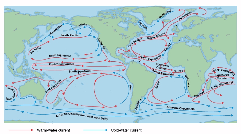
Cite this article
Link, J.S., Marshak, A.R. Characterizing and comparing marine fisheries ecosystems in the United States: determinants of success in moving toward ecosystem-based fisheries management. Rev Fish Biol Fisheries 29, 23–70 (2019). https://doi.org/10.1007/s11160-018-9544-z
Received:
Accepted:
Published:
Issue Date:
DOI: https://doi.org/10.1007/s11160-018-9544-z