On forms, cohomology and BV Laplacians in odd symplectic geometry

Abstract

We study the cohomology of the complexes of differential, integral and a particular class of pseudo-forms on odd symplectic manifolds taking the wedge product with the symplectic form as a differential. We thus extend the result of Ševera and the related results of Khudaverdian–Voronov on interpreting the BV odd Laplacian acting on half-densities on an odd symplectic supermanifold. We show that the cohomology classes are in correspondence with inequivalent Lagrangian submanifolds and that they all define semidensities on them. Further, we introduce new operators that move from one Lagragian submanifold to another and we investigate their relation with the so-called picture changing operators for the de Rham differential. Finally, we prove the isomorphism between the cohomology of the de Rham differential and the cohomology of BV Laplacian in the extended framework of differential, integral and a particular class of pseudo-forms.

1 Introduction

In this paper, we focus on the geometry of forms on odd symplectic (super)manifolds, which provide the mathematical framework for a geometrization of the Batalin–Vilkovisky (henceforth BV) quantization, see the groundbreaking [1, 23, 34], the more recent [20, 21, 26] for a thorough introduction to the subject. This very special class of supermanifolds are characterized by an odd 2-form $\omega$ which shares some properties with the ordinary symplectic form on a commutative even dimensional symplectic manifold and it can be used to define a Poisson-like bracket, called anti-bracket in the BV formalism. Our starting point, though, is the crucial observation of Ševera [33] that since $\omega$ is odd, it can be lifted to a nilpotent differential acting on forms (by wedge product), and it therefore makes sense to study its cohomology. In particular, we study the cohomology of $\omega$ for the complexes of differential, integral and a particular class of pseudo-forms on a generic odd symplectic supermanifolds and we show that classes in this cohomology are related to inequivalent Lagrangian submanifolds in the odd symplectic supermanifolds, see again [34]. The contact with BV formalism is made showing that all of these classes define semidensities on the odd symplectic supermanifold, where the Khudaverdian’s BV Laplacian acts (see [20] where the BV Laplacian is introduced geometrically via supergeometry and also [22], in relation to [33]). Further, we introduce new operators which relate different cohomology classes, which is equivalent to jump from one Lagrangian submanifold to another. This kind of operators are known in string theory as picture changing operators (PCO’s); they are usually introduced in connection with the de Rham differential and their use in supergeometry can be traced back to Belopolsky, see [2, 3, 12, 13] and below for a brief explanation: we show that these newly constructed PCO’s, acting on the cohomology of $\omega$, are related to the PCO’s of the de Rham differential by similarity transformations.

Another simple, yet amazing, observation in [33], is that the de Rham differential d and the odd symplectic form $\omega$ (anti)commute, making the de Rham complex into a double complex having d and $\omega$ as differentials. This remarkable fact implies that the Khudaverdian BV Laplacian [20,21,22,23,24] arises naturally—and invariantly—as the last nonzero differential in the related spectral sequence starting with $\omega .$ We broaden this analysis to the extended de Rham complex comprising differential, a particular class of pseudo- and integral forms. Further we study directly the cohomology of the BV Laplacian, by showing its homotopy—whose explicit form does not appear in the literature to the best knowledge of the authors. Finally we compare the two spectral sequences—the one starting with $\omega$ which computes the cohomology of the BV Laplacian and the one starting with d which computes the de Rham cohomology. We realize explicitly the isomorphism between these two cohomology in two ways, one of which makes use of the previously introduced picture changing operators for $\omega$ and d.

Finally, the last part of the paper is more speculative. Using some of the ingredients introduced in the paper, we argue an analogy between ordinary complex geometry and odd symplectic geometry: within this framework, we show how to write down an action for a Kodaira–Spencer-type theory [7] in the context of odd symplectic supermanifolds. This result is evocative, but it still requires a deep investigation, which we leave to future works.

Before we actually start, a brief explanation of the geometry of forms and related integration theory on supermanifolds and its historical development is in order¹. It has indeed been discussed in several studies that the geometry of forms and their complexes on supermanifolds proves to be remarkably richer compared to its counterpart on an ordinary purely commutative manifold (see [10, 13, 25] in the references and Th.Th. Voronov’s papers therein, for example, [35, 39, 40], just to mention some). The generalization of differential forms, i.e. polynomial functions in the $\hbox {d}x$’s and the $\hbox {d}\theta$—that in physical community are often called superforms—can indeed integrated only on bosonic purely even submanifolds of the supermanifold. In order to have a coherent integration theory that accounts for the odd directions characterizing a supermanifold, differential forms need thus to be supplemented by the so-called integral forms, whose complex were introduced by Bernstein and Leites in [5] as to incorporate Berezin’s volume forms. But this is not the end of the story: Bernstein and Leites [6] introduced indeed also pseudo-differential forms or pseudo-forms for short, which are by definition arbitrary functions of the $\hbox {d}x$’s and the $\hbox {d}\theta$’s. Requiring pseudo-forms to be “rapidly vanishing” at infinity in the $\hbox {d}\theta$’s, allows one to use them to integrate over sub-supermanifolds. Bernstein–Leites pseudo-forms don’t carry any grading in general: instead, a theory of forms graded by (super)dimensions p|q (were p is an integer and q run from zero to the fermionic dimension of the supermanifold) was developed by Voronov and Zorich in the 1980s [35,36,37] and further by Voronov in the 1990s and subsequent years [38,39,40].

A particular class of pseudo-forms is that given by functions of $\hbox {d}x$’s and $\hbox {d}\theta$’s which are supported in zero in the $\hbox {d}\theta$’s. These prove of crucial importance in many applications to strings and quantum field theory, see, for example, [2, 4, 14,15,16,17, 27] and the recent very terse review given by Witten, with stringy physics applications in mind, in [41]. In the following, we limit our analysis to this particular kind of pseudo-forms: in view of this, [41] might be taken as the source of notations and conventions. It is important to stress that, with abuse of notation, we will still refer simply as pseudo-forms to this particular specific class of the way more general pseudo-forms mentioned above: notice that the same convention is employed also in [41], where the author indeed underline that this terminology differs from the literature. This class of pseudo-forms can be given a grading, by the form degree and the so-called picture. In particular, in this context, one can see that pseudo-forms having maximal picture are integral forms, and indeed govern integration on sub-supermanifolds of codimension r|0 in supermanifolds of dimension p|q for $r \le p$. The usage of the term picture can create some confusion, though: therefore we provide with a brief explanation. This notion comes from the early days of string theory: different pictures represented different Fock spaces for the string states. In the fundamental paper [18], it was shown that the choice of a picture corresponds to a choice of ghost vacuum and each of these ghost vacuum leads to a different BRST complex and hence a different description of the physical states; in turn, these different descriptions can be related by “changing the picture”. Connection between this physical framework, rooted in conformal field theory, and the supergeometric framework was made explicit and brought to the attention of the physical community by Belopolsky (see [2, 3]), who considered a “singularization” of the r|s-forms introduced by Voronov and Zorich on p|q-dimensional supermanifolds (see above). In this context, the analog of the BRST operator is the de Rham differential, which does not change the value of s, thus splitting the full de Rham complex $\Omega ^{r|s}$ into $q+1$ subcomplexes: these subcomplexes are referred as pictures and the operations that move from one of these complexes to another as picture changing operators. It is fair to stress that the work of Witten, that we have indicated as reference above, builds upon Belopolsky’s papers, which should therefore be considered as crucial references of the present papers.

Another important aspect has to be underlined about the class of pseudo-forms we are dealing with: their global mathematical definition on a supermanifold is actually troublesome. Indeed, while differential (super)forms and integral forms are sections of vector bundles on a supermanifolds, pseudo-forms—in the sense used in [41] and in this paper—are in general not. More in particular, one can see that changing coordinates forces to give up (at least) the corresponding sheaf of pseudo-forms to be finitely generated—even if the diffeormorphism preserve the form degree and the picture: this can be easily realized by looking at low-dimensional examples, such as a 1|2-dimensional projective superspace, see again [41] or [8, 13, 28, 29]. This is a serious problem that plagues the theory. For this reason, it is fair to warn the reader that there is an unavoidable degree of formality in the results concerning these classes of pseudo-forms. Nonetheless, awaiting for a firmer mathematical ground, it is interesting to study these classes of pseudo-forms employing methods and instruments inspired by physics, such as the so-called picture changing operators, whose usage in supergeometry has been prompted by Belopolsky [2], as briefly sketched above. This point of view is taken in the present paper especially in Sect. 4 and some part of Sect. 5. Finally, let us mention that it would be very interesting to extend the present analysis to all the pseudo-forms, and not just the class in consideration here: this is of course a difficult task, which is outside the scope of the present paper, and we leave it to future endeavours.

2 Basics of supermanifolds and odd symplectic geometry

Before we start, we fix our notations. We let M and be an ordinary smooth manifold and a smooth supermanifold, respectively. If M is of dimension n, locally, we describe it by means of a chart $(U, x^i)$ for $i= 1, \ldots , n$ and U and open set in the topological space underlying M. Likewise, if is of dimension n|p, locally, we describe it by means of a chart of both even x and odd coordinates $\theta$ given by $(U, x^i | \theta _\alpha )$ for $i=1, \ldots , n$ and $\theta _\alpha = 1, \ldots , p.$ As it is customary, we will call the reduced space—i.e. the ordinary manifold—underlying . Also, given a supermanifold of dimension n|p we denote and the tangent bundle and its parity changed version: notice that these have rank n|p and p|n, respectively, being they locally generated by the derivations $\{ \partial _{x^i} | \partial _{\theta _\alpha } \}$ and $\{\pi \partial _{\theta _\alpha } | \pi \partial _{x^i}\}$, respectively. The dual of these bundles are given by and : here we will only use the second one, which is of rank p|n and locally generated by $\{ \hbox {d}\theta _\alpha | d x^i \}$ and we will denote it simply as or . The Berezinian bundle of a supermanifold is defined to be this is of parity $(p+q)\text{ mod }\, 2.$ The reader is invited to refer to [11, 25] or the recent [8, 9] for details.

Also, in order to relate the theory of forms with integration theory over supermanifolds, the ordinary de Rham complex needs to be extended by the so-called integral and pseudo-forms, which supplement ordinary differential forms in . Given a supermanifold of dimension n|q, these “generalized” forms are labelled by a number, called picture p, for $p=1, \ldots , q$, and for this reason, we will denote this extended de Rham complex by . Usual differential superforms are sections of and control integration over submanifolds of codimension k|q in , integral forms have maximal picture, i.e. are sections of and control integration over sub-supermanifolds of codimension k|0, while pseudo-forms are section of for $p \ne \{ 0, q\}$ and control integration over more general sub-supermanifolds of codimension k|l for $l \ne \{ 0, q\}.$ In this framework, forms in , for $p=0, \ldots , q$ can be seen as generalized functions over —this point of view is highlighted in [41]. Differential forms, in picture $p=0$, are characterized by a polynomial dependence of all of the even fibre coordinates $\hbox {d}\theta$’s, pseudo-forms with picture $0< p < q$ are characterized by Dirac delta distributional dependence on p out of the q $\hbox {d}\theta$’s, while the remaining $q-p$ are allowed a polynomial dependence. Finally, integral forms, having maximal picture $p = q$, have distributional dependence on all of the $\hbox {d}\theta$’s. Notice also that any is a -module and also -modules, i.e. any pseudo- and integral forms can be multiplied not only by functions but also by differential forms in for any n. The de Rham differential can be generalized as to operate in this extended framework, so that thus giving a “stack” of q complexes for $p=0, \ldots q$. This is represented by the following diagram

(2.1)

The (local) operators ${\mathbb {Y}}$ and ${\mathbb {Z}}$ moving vertically between complexes labelled by different pictures are called picture changing operators and have made their first appearance in a supergeometric context in [2]. Further explanations and examples of this kind of operators will be provided in the following.

2.1 Odd symplectic supermanifolds

In this paper, in particular, we will deal with a special class of supermanifolds, the so-called odd symplectic supermanifolds. These are defined as pairs , where is a supermanifold and is d-closed, i.e. $\hbox {d}\omega = 0$, odd and non-degenerate, i.e. it can be represented as $\omega \lfloor _{U} = \sum _{i, \alpha =1}^n \omega _{i\alpha } (x, \theta ) \hbox {d}x^i \wedge \hbox {d}\theta _\alpha$ in local coordinates $(U, x^i| \theta _\alpha )$, with $\omega _{i\alpha }$ an invertible matrix taking values on Notice that requiring $\omega$ to be non-degenerate constraints to have the same number of even and odd dimensions, i.e. an odd symplectic supermanifolds is always of dimension n|n for some n. These class of supermanifolds has been fully characterized by Schwarz in [34].

Theorem 2.1

(Schwarz [34]) Let be an odd symplectic supermanifold, with reduced manifold Then one has

• (1) in the neighbourhood $U_p$ of any point p in there exist a system of local coordinates $(U_p, x^i | \theta _i)$ such that $\omega = \sum _{i=1}^n dx^i \wedge d \theta _i$;

• (2) there exists a global symplectomorphism where $\omega _{std} = \sum _i dx^i \wedge d\theta _i$.

The first point in the above theorem proves the existence of Darboux coordinates also in this supersetting, while the second point provides a global description of the geometry of odd symplectic supermanifolds: up to symplectomorphisms, odd symplectic supermanifolds are all total spaces of odd cotangent bundle of some ordinary manifold M. It is therefore not restrictive to limit to this kind of geometries only.

More in details, an odd symplectic supermanifold $\text{ Tot } (\Pi {\mathcal {T}}^*_M) {:}{=}\Pi {\mathcal {T}}^*_M {\mathop {\rightarrow }\limits ^{\pi }} M$ will be characterized as follows: its underlying reduced manifold coincides with M and its structure sheaf is given by $(S^\bullet \Pi {\mathcal {T}}_M)^*$, i.e. functions of $\text{ Tot } (\Pi {\mathcal {T}}^*_M)$ are polynomial functions over the fibres ${\mathcal {T}}_{M, p}^*$. This means that if $(U, x^i)$ is a chart over M, then $(U, x^i | \theta _i)$ is a chart over $\text{ Tot } (\Pi {\mathcal {T}}^*_M)$, where the odd coordinates $\theta _i$ are given by $\theta _i {:}{=}\partial _{\hbox {d}x^i}.$ Notice that this implies that in an intersection $U \cap V$, of charts $(U, x^i|\theta _i)$ and $(V, y^i|\psi _i)$ one has that $\theta _i = \sum _{j=1}^n (\partial _{x^i} y^j )\psi _j$, i.e. the odd coordinates $\theta _i$ transform with the (transpose) inverse Jacobian of the change of coordinates $x^i \mapsto y^i$ over the base M.

Let us now look at forms over the odd symplectic supermanifold, that for notational convenience we will write as $\Pi {\mathcal {T}}^*M {:}{=}\text{ Tot } (\Pi {\mathcal {T}}^*_M)$. On a geometrical ground, $\Omega ^1_{\Pi T^*M}$ can be seen to be an extension of $\displaystyle \Omega ^1_{\Pi T^*M / M}$ by $\pi ^*\Omega ^1_M$, where $\pi : \Pi {\mathcal {T}}^*M \rightarrow M$ via the (canonical) short exact sequence

(2.2)

Since we are working over a smooth manifold M, these vector bundles are fine sheaves (of ${\mathcal {O}}_M$-modules) and therefore acyclic. It follows that, in particular, $Ext^1 ( \Omega ^1_{\Pi T^*M / M}, \pi ^*\Omega ^1_M) \cong 0$, and the short exact sequence (2.2) is (non-canonically) split, i.e. $\Omega ^1_{\Pi T^*M} \cong \pi ^*( \Omega ^1_M \oplus \Omega ^1_{\Pi T^*M / M} )$ (notice, incidentally, that this is equivalent to say that there exists a non-canonical reduction of the structure group Sp(n|n) preserving $\omega$ to $GL(n) \times GL (n)$). From the expressions of the transition functions for the local coordinates $x^i | \theta _i$ of the odd symplectic manifold one can then easily find the transition functions for the local generator $\hbox {d}\theta _i$ and $\hbox {d}x^i$ of $\Omega ^1_{\Pi {\mathcal {T}}^*M}$: these reads $\hbox {d}x^i = \sum _{j=1}^n \hbox {d}y^j (\partial _{y^j} x^i)$ and $\hbox {d} \theta _i = \sum _{j=1}^n (\partial _{x^i} y^j ) \hbox {d}\psi _j + \sum _{j=1}^n d (\partial _{x^i} y^j )\psi _j$. The non-diagonal part in transition functions of the $\hbox {d}\theta$’s is the typical feature of an extension of vector bundles: the splitness of (2.2) implies that coordinates can be found as to reduce the transformation of the $\hbox {d}\theta$’s to $\hbox {d} \theta _i = \sum _{j=1}^n (\partial _{x^i} y^j ) \hbox {d}\psi _j$. Clearly, the same would not be true in case the reduced manifold is a complex manifold or an algebraic variety.

Notice that this can also be seen from the interpretation of the Berezininan bundle via (dual of the) Koszul complex related to the tangent bundle of a supermanifold. Without giving further details, given a generic supermanifold , which is not necessarily an odd symplectic supermanifold, the only non-trivial representative in the related cohomology is given by : this class transforms with the (inverse) Berezinian of the Jacobian of the change of coordinates, i.e. as a generating section of . It follows that one gets a cohomological characterization of the Berezinian via the Koszul complex construction, which non-trivially generalizes the analogous construction for $\det (M)$ from the ordinary Koszul complex (in this respect, the Koszul complex appear first in supergeometry in the work by Penkov and Ogievetskii [31, 32], which is reported by Manin in [25]. See also the recent [30] for a self-contained treatment). It is then easy to verify, using the transition functions given above (and their dual) that in the case of an odd symplectic supermanifold the class $[\hbox {d}x^1 \ldots \hbox {d}x^n \otimes \partial _{\theta _1} \ldots \partial _{\theta _n}]$ transforms with the second power of the canonical bundle over M,  indeed in the (class of the) tensor product above the bit $\partial _{\theta _1} \ldots \partial _{\theta _n}$ transform exactly as $\hbox {d}x^1 \ldots \hbox {d}x^n.$

3 The cohomology of the odd symplectic form

As can be easily seen from the previous considerations, the odd symplectic form $\omega$ is invariant under generic change of coordinates and, being odd, it is nilpotent. It follows that multiplication by $\omega$ can be seen as an odd nilpotent morphism from to itself since all of these are sheaves of -modules. In other words, given the extended de Rham complex as above, we have another complex , which is characterized by the multiplication by $\omega$, i.e. $\alpha \mapsto \omega \alpha$, as nilpotent differential. In [33], Ševera showed that forms a bicomplex and proved that the cohomology is (naturally) isomorphic to semidensities on see [22, 33].

In this section, we start by revising the result in [33] and we extend it to the whole extended de Rham complex . Let us look at an ordinary differential superform at picture $p=0$ of any degree, we call it $\alpha _{0}$. Notice that $\alpha _0$ is locally of the form $\alpha _0 = f(x, \theta ) (\hbox {d}x^1)^{\epsilon _1} \ldots (\hbox {d}x^n)^{\epsilon _n} d \theta _1^{k_1} \ldots \hbox {d} \theta _n^{k_n}$ for $k_i \in {\mathbb {N}}_0$ and $\epsilon _i \in \{ 0,1\}.$ In this case, a homotopy for $\omega$ is given by the “counting” operator , locally given by . An easy calculation yields

(3.1)

where $\deg _{\hbox {d}\theta } (\alpha _0)$ is the even degree, i.e. $\deg _{\hbox {d}\theta } = \sum _{i=1}^n k_i$ of $\alpha _0$ and $\deg _{\hbox {d}x} (\alpha _0)$ is the odd degree, i.e. $\sum _{i = 1}^n \epsilon _i$ of $\alpha _0.$ It follows that the only instance in which the homotopy fails is $\deg _{\hbox {d}\theta } (\alpha _0) = 0$ and $\deg _{\hbox {d}x} (\alpha _0) = n$, that is for elements in of the form $\alpha _0 = f (x,\theta ) \hbox {d}x^1 \ldots \hbox {d}x^n$. Notice that this elements is indeed a cycle and therefore defines a class in cohomology. Using the above transformation properties, it is straightforward to verify that elements in this cohomology class transform as a semidensities, i.e. like sections in : in the case of an odd symplectic supermanifold one has that , which proves the claim.

Let us now move to maximal picture $p=n$ and consider the case of integral forms. Before we go, we recall that a generic integral form $\alpha _q$ can be written locally in the form $\alpha _q = f(x,\theta ) (\hbox {d}x^1)^{\epsilon _1} \ldots (\hbox {d}x^n)^{\epsilon _n} \delta ^{(\ell _1)} (\hbox {d}\theta _1) \ldots \delta ^{(\ell _n)} (\hbox {d}\theta _n)$, again for $\epsilon _i \in \{ 0,1\}$ and $\ell _i \in {\mathbb {N}}_0$ and since there are all of the $\delta (\hbox {d}\theta )$’s there cannot be any $\hbox {d}\theta$’s. Once again, the homotopy introduced above does the job, and one gets

(3.2)

where we have further defined $\deg _{\delta (\hbox {d}\theta )} (\alpha _n) = \sum _{i=1}^n \ell _i$. It follows that the homotopy fails in the case that $\deg _{\hbox {d}x} (\alpha _n)$ and $\deg _{\delta (\hbox {d}\theta )} (\alpha _n)$ are both zero, corresponding to the integral form of degree zero given by which is readily verified to be a cycle. It is once again not hard to see from this expression—using the transformation properties of the delta’s and of the $\hbox {d}\theta$’s—that it transforms as a section of $\det (M)$, i.e. it is once again a semidensity. Another way to see this, is to exploit the different representation of integral forms as sections of , see [13, 25] for explicit example of this correspondence. Up to the function $f (x, \theta )$, the form $\alpha _n$ corresponds to the section ${\mathcal {D}} (x,\theta ) \otimes \pi \partial _{x^1} \ldots \pi \partial _{x^n}$, where ${\mathcal {D}} (x,\theta )$ is a generating section of and $\pi \partial _{x^1} \ldots \pi \partial _{x^n}$ is a section in , which is totally anti-symmetric and it transforms as a section of the anti-canonical bundle $\det (M)^{\otimes -1}$. Just by looking at the above transformation properties, one has that that $\alpha _n$ transforms as a section in

Finally, let us deal with the case of our class of pseudo-forms, which—as usual—are the most delicate due to their problematic (global) definition, which impedes a fully satisfactory mathematical analysis. We recall that a generic pseudo-form $\alpha _p$ at picture $0< p < n$ is locally written as $\alpha _p = f (x, \theta ) (\hbox {d}x^1)^{\epsilon _1} \ldots (\hbox {d}x^n)^{\epsilon _n} \hbox {d}\theta _{i_1}^{k_{i_1}} \ldots \hbox {d} \theta _{i_{n-p}}^{k_{i_{n-p}}} \delta ^{(\ell _{j_1})} (\hbox {d}\theta _{j_1}) \ldots \delta ^{(\ell _{j_p})} (\hbox {d}\theta _{j_p})$, where any of the $i_s$ is different from any of $j_s$, i.e. a single $\hbox {d}\theta$ has either polynomial dependence or distributional. The homotopy we introduced above yields

(3.3)

where now $\deg _{\delta (\hbox {d}\theta )} (\alpha _p) = \sum _{s=1}^{n-p} \ell _{i_{s}}$ and $\deg _{\hbox {d}\theta } (\alpha _p) = \sum _{s=1}^p k_{j_s}$. Restricting to cocycles, one finds that $\deg _{\delta (\hbox {d}\theta )} (\alpha _p) = 0$ and that $\hbox {d}x^{j_s} = 0$ for any $s = 1, \ldots p$ so that $\deg _{\hbox {d}x } (\alpha _p) = \sum _{s = 1}^{n-p} \epsilon _{i_s}$, i.e. the remaining non-vanishing $\hbox {d}x$’s are those having the same indexes of the polynomial $\hbox {d}\theta$’s appearing. On the other hand, one has that compatibility with the previous equation forces $\sum _{s=1}^{n-p} \epsilon _{i_s} k_{i_s} = 0$, which implies that $k_{i_s} = 0$ for any $i_s$ so that $\deg _{\hbox {d}\theta } (\alpha _p) = 0$. This leads to elements of the following form . It can be seen that all of these belong to the same class and, once again, they all transform as semidensities, i.e. they transform with . We defer these checks to “Appendix”.

Further, it is not hard to see that the de Rham differential d is zero everywhere on the cohomology of $\omega$, since for any $p=0, \ldots n$, the de Rham differential always moves out to a space where the cohomology of $\omega$ is zero.

We recollect these results in the following theorem.

Theorem 3.1

(Cohomology ) Let be an odd symplectic supermanifold of dimension n|n and let for $p = 0, \ldots n$ be its extended de Rham double complex. Then the following are true:

• (1) is generated by $\sum _{i_{1}, \ldots , i_n}\epsilon _{i_1 \ldots i_n} dx^{i_1} \ldots dx^{i_{n-p}} \delta (d\theta _{i_{n-p+1}}) \ldots \delta (d\theta _{i_{n}})$ over In particular, so that

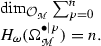
• (2) Let for any $p = 1, \ldots n.$ Then is isomorphic to semidensities on

• (3) The de Rham differential vanishes on all the cohomology of $\omega$. In particular for any $p=0,\ldots , n$.

As already said above, the case $p=0$ has been discussed by Ševera [33]. Also, notice that in the theorem we have chosen $\sum _{i_{1}, \ldots , i_n}\epsilon _{i_1 \ldots i_n} \hbox {d}x^{i_1} \ldots \hbox {d}x^{i_{n-p}} \delta (\hbox {d}\theta _{i_{n-p+1}}) \ldots \delta (\hbox {d}\theta _{i_{n}})$ as representative for symmetry reason, but—as explained above—we might have chosen just one element in this sum.

3.1 Lagrangian submanifolds and cohomology

In this subsection, we want to outline a connection of the previous results with Lagrangian submanifolds in an odd symplectic supermanifold . Notice that since the term sub-supermanifolds is quite clumsy, we refer at them as submanifolds instead. In particular, one defines a Lagrangian submanifold of to be one that is maximally isotropic. This means that, given an embedding , we require that $\iota ^*\omega = 0$ and that is not a proper submanifold of any other isotropic submanifold of . Once again, the geometry of these special submanifolds has been characterized by Schwarz.

Theorem 3.2

(Schwarz [34]) Let be an odd symplectic supermanifold, with reduced manifold and let be a Lagrangian submanifold in Then there exists a pair , where is an ordinary manifold and is the symplectomorphism of Theorem 2.1, such that where is the odd conormal bundle of .

This theorem says that—once again up to global symplectomorphisms—the geometry of a Lagrangian submanifold in an odd symplectic supermanifold is constrained to be the one of the total space of a conormal bundle in Notice that given an ordinary manifold M the odd conormal bundle of a submanifold $\iota : L \hookrightarrow M$ is defined to be the bundle whose fibres are forms which give zero on vectors in $\Pi {\mathcal {T}}_L$, i.e. $\Pi {\mathcal {T}}^*_{M/L}$ fits in the (split, in the smooth case) short exact sequence

(3.4)

Since the rank of the odd conormal bundle corresponds to the odd dimension of the related Lagrangian submanifold , this constraints any Lagrangian submanifold in to be of dimension $k| n-k$ if M is of dimension n (hence of dimension n|n) and L is of dimension k. For example, let us consider the example of an odd symplectic supermanifold of dimension (2|2) given by with its standard odd symplectic form $\omega = \sum _{i=1}^2 \hbox {d}x^i \hbox {d}\theta _i$, and look at its Lagrangian submanifolds. The first corresponds to the reduced manifold, , i.e. it is given by the locus which singles out a 2|0-dimensional (super)manifold. The second is given by the “complement” of in , that is , which is a 0|2-dimensional supermanifold. Then we have two obvious 1|1-dimensional sub-supermanifolds, which are given by the loci and in $,$ notice by the way that this two Lagrangian submanifolds are connected by a symplectomorphism. In particular, for $t \in [0,1]$, the transformation $G_t = \text{ diag } (A(t), A^\intercal (t)) \in SO(2) \times SO(2)$ with

$$\begin{aligned} A(t) = \left( \begin{array}{cc} \cos (\frac{\pi }{2} t) &{} \quad -\sin (\frac{\pi }{2} t) \\ \sin (\frac{\pi }{2} t) &{} \quad \cos (\frac{\pi }{2} t) \end{array} \right) \end{aligned}$$

(3.5)

rotates the Lagrangian to . We say that two Lagrangians are Lagrangian-homotopic if there exists a smooth family of Lagrangians for $t \in [0,1]$ that relate them. This is just the case above: the flow along $G_t$ for $t \in [0,1]$ defines a smooth family of Lagrangian submanifolds such that and This defines an equivalence relation, we will write and denote the corresponding class with . The above example can be generalized to any ${\mathbb {R}}^n$, though it is fair to stress that, in general, classification of Lagrangian submanifolds is a delicate and difficult problem, intimately related to topology, and we will not dwell any further in it for it is not the aim of the present paper.

Now let be the parity reversed tangent bundle of a certain Lagrangian submanifold. It can be seen that one has a splitting , for a certain Lagrangian complement of in . In this instance, the related Berezinian bundles, i.e. and are isomorphic—notice by the way that this is not at all trivial, see [33] for a discussion. On the other hand, one has that and the splitting yields , so it can be concluded that for any Lagrangian submanifold embedded into This means that any Lagrangian submanifold in an odd symplectic supermanifold is such that its Berezinian transforms as the square root of the Berezinian of , i.e. as a semidensity on .

Restricting to the case of contractible spaces or simply ${\mathbb {R}}^n$, by the above considerations one finds that the class corresponds to the tensor density of the class of Lagrangian submanifolds of dimension $n-p|p$, which is indeed a semidensity; conversely to the class , one associates the corresponding class into . An immediate example is given by the class of , corresponding to the Lagrangian submanifold , and by its complement in , which is a purely odd supermanifold (over a point) of dimension 0|n and whose class is . Notice that one has , i.e. the tensor product of two semidensities—which are Lagrangian complement of each other—yields a density for the odd symplectic supermanifold , as explained above.

4 Picture changing operators and Lagrangian submanifolds

As reported in Introduction, interesting objects in the context of the extended de Rham complex are the so-called picture changing operators (PCO’s for short), which have been introduced first in a supergeometric context by Belopolsky [2] in relation to issues arising in superstring perturbation theory. As their name suggests, and briefly addressed above, these are operators that allow one to move “vertically” (or diagonally) in the diagram (2.1). More in particular, as they act on sections of , they either increase or decrease the picture p and can only be characterized as local operators related to a certain direction singled out by a vector field in . They are better behaved when looked as operators related to the cohomology with respect to some differential; indeed, they are constructed as to respect cohomology classes, i.e. they maps cocycles to cocycles and coboundaries to coboundaries. The interested reader can find details in the recent [13], where PCO’s with respect to the de Rham differential d are discussed. As sketched above, these kind of operators and their properties are related to the corresponding operators defined in conformal field theory, more in particular in the context of bosonization and fermionization, and for this reason, the reader should be warned that, to date, it does not exists a fully mathematically satisfactory theory of the PCO’s yet. Nonetheless, similarly to the ill-defined path integrals in QFT’s, it can be seen that the machinery provided by the PCO’s lead in very economic way to many results that can be proved to be mathematically correct. Within these stated limits, in the present section we are interested in constructing and interpreting the PCO’s with respect to $\omega$ seen as a differential as above. Inspection of the non-trivial cohomology classes suggests how to define a picture raising operator. Namely working in a coordinate chart given by $x^i | \theta _i$ for $i = 1, \ldots , n$, one defines

(4.1)

where $\delta ^j_i$ is the Kronecker symbol and it stands for a (conventional) choice of the direction of the PCO. In other words, the action of the picture raising operator ${\mathbb {Y}}$ is to replace $\hbox {d}x^i$’s with the corresponding $\delta (\hbox {d}\theta _i)$’s. Notice in particular that ${\mathbb {Y}}$ is an even derivative of for any p and, remarkably, it preserves cohomology classes (indeed it can be checked that it commutes with $\omega$), so that one obtains a map In particular, acting with the “product” of n picture raising operators one gets a map from the cohomology of differential forms to the cohomology of integral forms, with $[ \hbox {d}x^1 \ldots \hbox {d}x^n ] \mapsto [ \delta (\hbox {d}\theta _1) \ldots \delta (\hbox {d}\theta _n) ]$. The definition of ${\mathbb {Y}}$ includes a conventional choice of a direction, that in (4.1) is encoded in the Kronecker symbol. Let us clarify this point: instead of using the identity matrix, we could ask whether it is possible to make a different choice in the definition (4.1), namely

$$\begin{aligned} {\mathbb {Y}} {:}{=}\sum _{i,j=1}^n \delta \left( \hbox {d} \theta _i \right) J_i^j \iota _j \ , \end{aligned}$$

(4.2)

for a certain matrix J (that a priori can be non-constant). If we want (4.2) to be compatible with the cohomology of $\omega$, we have to require that it commutes with $\omega$, namely $[{\mathbb {Y}}, \omega ]= 0$, which implies

$$\begin{aligned} \sum _{i,j,k,l=1}^n \delta \left( \hbox {d} \theta _i \right) J_i^j \iota _j \left( \hbox {d}x^k \omega ^l_{\; k} \hbox {d} \theta _l \right) = \sum _{i,j,l=1}^n \delta \left( \hbox {d} \theta _i \right) J_i^j \omega ^l_{\; j} \hbox {d} \theta _l = 0 \ . \end{aligned}$$

(4.3)

If we consider $\omega ^l_j = \delta ^l_j$, then Eq.  (4.3) simply implies that J is diagonal, and hence, it has n free entries, exactly as a vector V. Therefore, we can trade the definition (4.2) for the equivalent

$$\begin{aligned} {\mathbb {Y}}_{V} {:}{=}\sum _{i,j=1}^n \delta \left( V^i \hbox {d} \theta _i \right) V^j \iota _j \ , \end{aligned}$$

(4.4)

where we have specified the dependence on V in order to distinguish it from (4.2). It is clear that (4.4) is a non-trivial map , since it commutes with $\omega$, really

$$\begin{aligned} {\mathbb {Y}}_{V} \omega = \sum _{i,j,k=1}^n \delta \left( V^i \hbox {d} \theta _i \right) V^j \iota _j \hbox {d}x^k \hbox {d} \theta _k = \sum _{i,j=1}^n \delta \left( V^i \hbox {d} \theta _i \right) V^j \hbox {d} \theta _j = 0 \ . \end{aligned}$$

(4.5)

It is easy to observe that different choices of the vector V in (4.4) or, equivalently, different choices of the (diagonal) matrix in (4.2), lead to cohomologically equivalent PCO’s. We postpone this discussion to the example in “Appendix”. We will use (4.1) as the definition of ${\mathbb {Y}}$, unless differently specified.

Analogously, picture lowering operators can be introduced. Working again in the chart $x^i | \theta _i$ for $i = 1, \ldots , n$, one defines, using the definition of $\Theta (\iota ^i)$ given in [13]

(4.6)

where $V_i$ is a constant vector encoding the conventional choice of a direction. When not differently specified, we choose $V_i = (1, \ldots , 1)$. The presence of $\Theta (\iota ^i)$² makes the action of this operator less manifest compared to the picture raising operator defined above. Let us consider as an example its action on $\alpha _n = f (x, \theta ) \delta (\hbox {d}\theta _1) \ldots \delta (\hbox {d}\theta _n)$, and for simplicity, let us consider $V_i = (0, \ldots , 0,1,0, \ldots ,0)$, i.e. the only non-trivial entry is the ith:

$$\begin{aligned} {\mathbb {Z}} \left( f \left( x , \theta \right) \delta (\hbox {d}\theta _1) \ldots \delta (\hbox {d}\theta _n) \right)&= f \left( x , \theta \right) \omega \wedge \left( \frac{1}{\hbox {d} \theta _i} \delta (\hbox {d}\theta _1)\ldots \widehat{\delta (\hbox {d}\theta _i)}\ldots \delta (\hbox {d}\theta _n) \right) \nonumber \\&= f (x, \theta ) \hbox {d}x^i \delta (\hbox {d}\theta _1)\ldots \widehat{\delta (\hbox {d}\theta _i)}\ldots \delta (\hbox {d}\theta _n), \end{aligned}$$

(4.7)

where ${\hat{\delta }}$ represents a delta not appearing in the expression: in other words, the action of the operator ${\mathbb {Z}}$ makes the ith delta drop and it get substituted with the corresponding $\hbox {d}x^i$. Notice also that in the previous calculation appears the formal expression $1/\hbox {d}\theta$, which in the language of string theory belongs to the large Hilbert space (see again [13]), but it drops at the ends of the calculation. Just like ${\mathbb {Y}}$ above, also ${\mathbb {Z}}$ is even and it preserves cohomology classes—once again it commutes with $\omega$. In analogy with what above, in particular, we have that , maps the cohomology of integral forms to the cohomology of superforms, i.e. $[\delta (\hbox {d}\theta _1) \ldots \delta (\hbox {d}\theta _n)] \mapsto [\hbox {d}x^1 \ldots \hbox {d}x^n]$. Finally, it follows easily that ${\mathbb {Z}} {\mathbb {Y}} = {\mathbb {Y}} {\mathbb {Z}} = 1$ in cohomology.

The above discussion, together with the considerations carried out in the previous sections about Lagrangian submanifolds in odd symplectic supermanifolds, yields a very nice geometrical interpretation of the action of the PCO’s. We have indeed seen that forms $[\alpha ]$ in the cohomology are related to inequivalent Lagrangian submanifolds in : the action of the PCO’s makes one jumps from one Lagrangian submanifold to another (inequivalent) Lagrangian submanifold. In other words, PCO’s does not act, geometrically, as symplectomorphisms of a Lagrangian submanifold in : from this point of view, they can be seen as non-trivial maps from the cohomology to itself, or analogously as maps between classes of Lagrangian submanifolds of different codimension in .

The PCO’s ${\mathbb {Z}}$ and ${\mathbb {Y}}$ defined above are related to the operator (multiplication by) $\omega$. We now aim at establishing a relation between these and the PCO’s related to de Rham differential d and constructed as to act on the cohomology classes , see [13]. In particular, in order to carry out this comparison, we will consider the following PCO’s for d: the picture raising operator ${\mathbb {Y}}^d$ is a multiplicative operator, formally written as ${\mathbb {Y}}^d {:}{=}\sum _{i=1}^n \theta _i \delta (\hbox {d}\theta _i)$, while the picture lowering operator is given by ${\mathbb {Z}}^{d} {:}{=}-i [d, \Theta (V_i \iota ^i)]$, see again [13] for a discussion. Notice in particular that ${\mathbb {Y}}^d$ and ${\mathbb {Z}}^d$ raises and lowers the picture of the form by one, respectively, while they leave the form number unchanged.

In the following of this section, we will write the PCO’s related to $\omega$ introduced above as ${\mathbb {Y}}^\omega$ and ${\mathbb {Z}}^\omega$, in order to distinguish them from those related to d.

Before we start, following the relation between the operator d and the total operator $d + \omega$ observed in [22], one can note that

$$\begin{aligned} D {:}{=}d + \omega = e^{\Sigma } d e^{-\Sigma }\,, \quad \quad I_i {:}{=}\iota _i - \theta _i = e^{\Sigma } \iota _i e^{-\Sigma }\,, \end{aligned}$$

(4.8)

where $\Sigma = \sum _{i=1}^n \hbox {d}x^i \theta _i$ is the Liouville form, which is defined so that $\omega = - d \Sigma = \sum _{i=1}^n \hbox {d}x^i \hbox {d}\theta _i$. In particular, the fact that the odd symplectic form $\omega$ is d-exact implies that $D^2 =0$. In addition, it is easy to check that $\{ I_i, I_j\} =0$ and

$$\begin{aligned} D I_i + I_i D = {{\mathcal {L}}}_i - ({{\mathcal {L}}}_i \Sigma )\,, \end{aligned}$$

(4.9)

where ${\mathcal {L}}_i$ is the Lie derivative along the coordinate vector field in the related direction. Notice that this can also be derived using the similarity transformation. By using $\left[ d , \Sigma \right] = - \omega$ and $\left[ \omega , \Sigma \right] = 0$, one can compute (we omit the sum symbols)

$$\begin{aligned} {\mathbb {Z}}^d - {\mathbb {Z}}^\omega= & {} -i \left[ d - \omega , \Theta (V_i \iota ^i)\right] = -i \left[ e^{-\Sigma } d e^{\Sigma }, \Theta (V_i \iota ^i) \right] \nonumber \\= & {} -i e^{-\Sigma } \left[ d , \Theta (V_i \iota ^i) \right] e^{\Sigma } = e^{-\Sigma } {{\mathbb {Z}}}^{d} e^{\Sigma } \ , \end{aligned}$$

(4.10)

since $[\Sigma ,\Theta (V_i \iota ^i)]=0$. Analogously we have

$$\begin{aligned} {\mathbb {Y}}^\omega - {\mathbb {Y}}^d= & {} \left[ \iota _i - \theta _i, \delta (\hbox {d}\theta _i)\right] = \left[ e^{\Sigma } \iota _i e^{-\Sigma }, \delta (\hbox {d}\theta _i) \right] \nonumber \\= & {} e^{\Sigma } \left[ \iota _i , \delta (\hbox {d}\theta \hbox {d}\theta _i) \right] e^{-\Sigma } = e^{\Sigma } {\mathbb Y}^{\omega } e^{-\Sigma } \,. \end{aligned}$$

(4.11)

Now, similarly as above, defining ${{\mathcal {R}}} = \sum _{i=1}^n \left( \partial ^i \iota _i + \partial _i \iota ^i \right)$, one can verify that $[{{\mathcal {R}}}, \omega ] = d$ and $\left[ {\mathcal {R}} , d \right] = 2 \Delta _{BV}$. This leads in turn to $d + \omega + 2 \Delta _{BV} = e^{{\mathcal {R}}} \omega e^{-{\mathcal {R}}}$ and $\theta _i - \iota _i = e^{{\mathcal {R}}} \theta _i e^{-{\mathcal {R}}}$ so that, using ${\mathcal {R}}$ instead of $\Sigma$ one sees that

$$\begin{aligned} {\mathbb {Z}}^d - {\mathbb {Z}}^\omega = e^{\mathcal {-R}} {\mathbb {Z}}^\omega e^{ {\mathcal {R}}}, \quad \quad {\mathbb {Y}}^\omega - {\mathbb {Y}}^d = e^{{\mathcal {R}}} {\mathbb {Y}}^d e^{-{\mathcal {R}}}, \end{aligned}$$

(4.12)

where we have implicitly used $\left[ {\mathcal {R}} , \Theta \left( V_i \iota ^i \right) \right] = 0$ and $\left[ \Delta _{BV} , \Theta \left( V_i \iota ^i \right) \right] = 0$. Together with (4.10) and (4.11), one has $e^{-\Sigma } {{\mathbb {Z}}}^{d} e^{\Sigma } = e^{\mathcal {-R}} {{\mathbb {Z}}}^{\omega } e^{{\mathcal {R}}}$ and $e^{\Sigma } {\mathbb Y}^{\omega } e^{-\Sigma } = e^{{\mathcal {R}}} {\mathbb {Y}}^{d} e^{-{\mathcal {R}}}$, so that

$$\begin{aligned} {\mathbb {Z}}^d&= (e^{\Sigma } e^{\mathcal {-R}}) {\mathbb {Z}}^\omega (e^{{\mathcal {R}}}e^{-\Sigma }) = e^{ \Sigma - {\mathcal {R}}} {\mathbb {Z}}^\omega e^{-\Sigma + {\mathcal {R}}},\nonumber \\ {\mathbb {Y}}^d&= (e^{-{\mathcal {R}}} e^{\Sigma }) {\mathbb {Y}}^\omega (e^{- \Sigma } e^{{\mathcal {R}}}) = e^{\Sigma - {\mathcal {R}}} {\mathbb {Y}}^\omega e^{- \Sigma + {\mathcal {R}}}, \end{aligned}$$

(4.13)

where we note that the product of the exponential can be rewritten as a unique exponential using the Baker–Campbell–Hausdorff formula, and the last equality follows from the commutation relation between $\Sigma$ and ${\mathcal {R}}$. Notice that the previous can interpreted as similarity transformations between the two pairs of PCO’s. As a consistency check, we notice that (4.13) is compatible with ${\mathbb {Y}} {\mathbb {Z}} = {\mathbb {Z}} {\mathbb {Y}} = 1$ (in cohomology), which is valid for the PCO’s relative to d and for those relative to $\omega$.

5 BV Laplacian on semidensities

In the previous sections, we have explained that to Lagrangian submanifolds are attached semidensities. In this context, for example, Ševera treated the special case of the reduced manifold , which is a Lagrangian submanifold in . Further, Ševera showed also that the invariance of the BV Laplacian introduced by Khudaverdian in [20, 21] follows from first principles. This operator is a certain differential—actually the second differential, in our convention and the third in Ševera’s—of the spectral sequence related to the double complex . 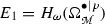Something is to be stressed before we go on, though, for the situation is peculiar. We take $\omega$ to be the vertical differential and $\delta _1 {:}{=}d$ to be the horizontal differential of the double complex, and defining $(E_{r}, \delta _r )$ the spectral sequence related to the vertical filtration, i.e. we first compute the cohomology with respect to $\omega$, so that : we have seen that when acting on $E_1$, the de Rham differential $\delta _1 = d$ is the zero map. This might lead to think that the spectral sequence converges already at page one, but this is not the case. Indeed, one finds that the differential $\delta _2$ acting on is not zero, and it is the discovery of Ševera in [33] that $\delta _2$ is indeed the BV Laplacian, $\Delta _{BV} = \sum _i \partial _{x^i} \partial _{\theta _i}$, which he writes formally as $\delta _2 = d \circ \omega ^{-1} \circ d$ to get the right “movement” for the second differential of the spectral sequence, $\delta _2 : E_{2}^{\bullet , \bullet } \rightarrow E_{2}^{\bullet +2,\bullet -1}$. This means that one finds naturally an invariant differential acting on semi-densities (generated by the element $[\hbox {d}x^1 \ldots \hbox {d}x^n] \in E_1$), corresponding to the first page $E_1$ of the spectral sequence, which is nothing but the BV Laplacian.

The previous analysis can be generalized to our extended framework considering for any p and the action of the second differential $\delta _2$ on the related cohomology groups. We start reviewing the $p=0$ case. One has that since d maps elements in to $\omega$-exact elements, i.e.

$$\begin{aligned} d \left( f (x, \theta ) \hbox {d}x^1 \ldots \hbox {d}x^n \right) = \omega \alpha _0^{(n-1)}, \end{aligned}$$

(5.1)

where . This is convenient, since the $\omega$ appearing in the (5.1) and the $\omega ^{-1}$ coming from $\delta _2$ cancel one another, leaving with $d\alpha _0^{(n-1)}$ to compute:

$$\begin{aligned} \delta _2 (f (x, \theta ) \hbox {d}x^1 \ldots \hbox {d}x^n)&= (-1)^{|f| +1} \sum _{i, j = 1}^n \hbox {d}x^j (\partial _{j} \partial ^i f (x, \theta )) \iota _i (\hbox {d}x^1 \ldots \hbox {d}x^n) \nonumber \\&= \sum _{i=1 }^n \partial _i \partial ^i f (x, \theta ) (\hbox {d}x^1 \ldots \hbox {d}x^n) + \left( \omega \text{-exact } \text{ terms } \right) . \end{aligned}$$

(5.2)

It follows that restricting the action of $\delta _2 = d \circ \omega ^{-1} \circ d$ on the cohomology of $\omega$, i.e. on semidensities attached to the Lagrangian submanifold corresponding to the reduced manifold, one finds indeed

$$\begin{aligned} \delta _2 \left( f(x, \theta ) [\hbox {d}x^1 \ldots \hbox {d}x^n] \right) = \sum _{i=1}^n \frac{\partial ^2}{\partial x^i \partial \theta _i} f (x, \theta ) [\hbox {d}x^1 \ldots \hbox {d}x^n]. \end{aligned}$$

(5.3)

now we show that this extends easily to any class in the full cohomology for any p. Let us start from integral forms: once again, the first observation is that

$$\begin{aligned} d (f (x, \theta ) \delta (\hbox {d}\theta _1) \ldots \delta (\hbox {d}\theta _n)) = \omega \alpha _n^{(-1)} \end{aligned}$$

(5.4)

for , and where we have used that $- \hbox {d}\theta _i \delta ^{\prime } (\hbox {d}\theta _i) = \delta (\hbox {d}\theta _i).$ So, just like above, we are left to compute $d\alpha ^{(-1)}_n$ from $\delta _2 (f \delta (\hbox {d}\theta _1) \ldots \delta (\hbox {d}\theta _n))$, and one gets

$$\begin{aligned} \delta _2 (f (x, \theta ) \delta (\hbox {d}\theta _1) \ldots \delta (\hbox {d}\theta _n))&= - \sum _{i, j =1}^n \hbox {d}\theta _j \partial ^j \partial _i f (x, \theta ) \iota ^i (\delta (\hbox {d}\theta _1) \ldots \delta (\hbox {d}\theta _n)) \nonumber \\&= \sum _{i=1}^n ( \partial ^i \partial _i f ) (\delta (\hbox {d}\theta _1) \ldots \delta (\hbox {d}\theta _n)) + \left( \omega \text{-exact } \text{ terms } \right) . \end{aligned}$$

(5.5)

Once again, this means that

$$\begin{aligned} \delta _2 \left( f(x, \theta ) [\delta (\hbox {d}\theta _1) \ldots \delta (\hbox {d}\theta _n) ] \right) = \sum _{i=1}^n \frac{\partial ^2}{\partial x^i \partial \theta _i} f (x, \theta ) [\delta (\hbox {d}\theta _1) \ldots \delta (\hbox {d}\theta _n)]. \end{aligned}$$

(5.6)

Finally, let us consider the case of pseudo-forms: as usual these represent the case where the most attention is required, as it is a mixture of the previous situations for superforms and integral forms. In particular, adopting the notation of the previous sections, considering the representative of a class at picture p given by $f_{a_1 \ldots a_n}(x, \theta ) \hbox {d}x^{a_1} \ldots \hbox {d}x^{a_{n-p}} \delta (\hbox {d}\theta _{a_{n-p+1}}) \ldots \delta (\hbox {d}\theta _{a_n})$ one first observe that

$$\begin{aligned} \hbox {d} \alpha _p&= \omega \sum _{i=1}^{n-p} (-1)^{|f|+1}\left( \partial ^{a_i} f_{a_1 \ldots a_n} (x, \theta ) \right) \iota _{a_i} \left( \hbox {d}x^{a_1} \ldots \hbox {d}x^{a_{n-p}} \delta (\hbox {d}\theta _{a_{n-p+1}}) \ldots \delta (\hbox {d}\theta _{a_n}) \right) + \nonumber \\&\quad - \omega \sum _{i = n-p+1}^{n} \left( \partial _{a_i} f_{a_1 \ldots a_n} (x, \theta ) \right) \iota ^{a_i} \left( \hbox {d}x^{a_1} \ldots \hbox {d}x^{a_{n-p}} \delta (\hbox {d}\theta _{a_{n-p+1}}) \ldots \delta (\hbox {d}\theta _{a_n}) \right) . \end{aligned}$$

(5.7)

Therefore, cancelling the $\omega$ with the $\omega ^{-1}$ coming from $\delta _2$, one is left with

$$\begin{aligned}&\delta _2 \left( f_{a_1 \ldots a_n}(x, \theta ) \hbox {d}x^{a_1} \ldots \hbox {d}x^{a_{n-p}} \delta (\hbox {d}\theta _{a_{n-p+1}}) \ldots \delta (\hbox {d}\theta _{a_n}) \right) \nonumber \\&\quad = (-1)^{|f|+1} \sum _{i=1}^{n-p} \hbox {d}x^{a_i} \left( \partial _{a_i} \partial ^{a_i} f_{a_1 \ldots a_n} (x, \theta ) \right) \iota _{a_i} \left( \hbox {d}x^{a_1} \ldots \hbox {d}x^{a_{n-p}} \delta (\hbox {d}\theta _{a_{n-p+1}}) \ldots \delta (\hbox {d}\theta _{a_n}) \right) \end{aligned}$$

(5.8)

$$\begin{aligned}&\qquad - \sum _{i=n-p+1}^{n} \hbox {d}\theta _{a_i} \partial ^{a_i} \partial _{a_i} f_{a_1\ldots a_n} (x, \theta ) \iota ^{a_i} \left( \hbox {d}x^{a_1} \ldots \hbox {d}x^{a_{n-p}} \delta (\hbox {d}\theta _{a_{n-p+1}}) \ldots \delta (\hbox {d}\theta _{a_n}) \right) + \ldots \end{aligned}$$

(5.9)

where the ellipses stand for $\omega$-exact terms. Summing up the pieces one has, up to exact terms

$$\begin{aligned}&\delta _2 \left( f_{a_1 \ldots a_n}(x, \theta ) \hbox {d}x^{a_1} \ldots \hbox {d}x^{a_{n-p}} \delta (\hbox {d}\theta _{a_{n-p+1}}) \ldots \delta (\hbox {d}\theta _{a_n}) \right) \nonumber \\&\quad = \left( \sum _{i = 1}^{n} \partial _i \partial ^i f_{a_1 \ldots a_n} (x, \theta ) \right) \hbox {d}x^{a_1} \ldots \hbox {d}x^{a_{n-p}} \delta (\hbox {d}\theta _{a_{n-p+1}}) \ldots \delta (\hbox {d}\theta _{a_n}) \end{aligned}$$

(5.10)

which shows that also in this case one finds

$$\begin{aligned}&\delta _2 \left( f_{a_1 \ldots a_n}(x, \theta ) [\hbox {d}x^{a_1} \ldots \hbox {d}x^{a_{n-p}} \delta (\hbox {d}\theta _{n-p+1}) \ldots \delta (\hbox {d}\theta _n) ] \right) \nonumber \\&\quad = \sum _{i=1}^n \frac{\partial ^2}{\partial x^i \partial \theta _i} f_{a_1 \ldots a_n} (x, \theta ) [\hbox {d}x^{a_1} \ldots \hbox {d}x^{a_{n-p}} \delta (\hbox {d}\theta _{n-p+1}) \ldots \delta (\hbox {d}\theta _n) ]. \end{aligned}$$

(5.11)

Now, one should evaluate the cohomology of the differential $\delta _2 = \Delta _{BV}$. The usual approach employed in literature is to map the BV Laplacian to the de Rham differential by means of the so-called odd Fourier transform [26], thus concluding—under suitable hypotheses—that the cohomology is just given by ${\mathbb {R}}$; this approach is understood in [33]. We will follow another approach, namely we directly compute the cohomology of $\Delta _{BV}$ by showing its homotopy operator, without making use of the odd Fourier transform: among other things, this provides one with the form of the representatives of this cohomology.

In particular, we claim that given a (local) section of the structure sheaf of , which we write $s = f^I(x) \theta _I$ for some multi-index I, then

$$\begin{aligned} f^{I} \theta _I \longmapsto h (f^I \theta _I) {:}{=}\sum _{a=1}^n \left( \int _{0}^1 \hbox {d}t \,t^{Q_s} x^a G^{*}_t f^I (x)\right) \otimes \theta _a \theta _I, \end{aligned}$$

(5.12)

where $G^{*}_t f (x) = f(tx)$ for $t \in [0,1]$, i.e. it is the pullback of the section s under the map $x {\mathop {\longmapsto }\limits ^{G_t}} t x$ and $Q_s$ is a constant depending on the section, to be determined later on. The tensor product is there for notational convenience (actually, one might have written $s = f^I (x) \otimes \theta _I$ from the very beginning). One has that

$$\begin{aligned} h \circ \Delta _{BV} (f^I (x) \theta _I) = \sum _{a,b=1}^{n} \left( \int _0^1 \hbox {d}t \, t^{Q_{\delta s}} x_b G^{*}_t (\partial _{x^a} f^I (x)) \right) \otimes \theta _b \partial _{\theta _a} \theta _I. \end{aligned}$$

(5.13)

On the other hand, one computes

$$\begin{aligned} \Delta _{BV} \circ h (f^I (x) \theta _I)&= \sum _{a=1}^n \int _0^1 \hbox {d}t \, t^{Q_s} G_{t} f^I(x) \otimes \theta _I \end{aligned}$$

(5.14)

$$\begin{aligned}&\quad - \sum _{a=1}^n \int _0^1 \hbox {d}t \, t^{Q_s} G^*_t f^I (x) \otimes \theta _a \partial _{\theta _a} \theta _I \end{aligned}$$

(5.15)

$$\begin{aligned}&\quad + \sum _{a=1}^n \int _0^1 \hbox {d}t \, t^{Q_s} x^a \partial _{x^a} (G^*_t f^I(x)) \otimes \theta _I \end{aligned}$$

(5.16)

$$\begin{aligned}&\quad - \sum _{a,b=1} \int _0^1 \hbox {d}t \, t^{Q_s} x_b \partial _{x^a} (G^*_t f^I (x)) \otimes \theta _b \partial _{\theta _a } \theta _I \end{aligned}$$

(5.17)

Let us examine the various summands. Clearly the first one is just $n \int _0^1 \hbox {d}t \, t^{Q_s} G_{t} f^I(x) \otimes \theta _I$, while the last term cancels with the term $h \circ \Delta _{BV}$ above, upon using the chain rule and posing $Q_{\delta s} = Q_s + 1.$ The second one can be rewritten as

$$\begin{aligned} \sum _{a=1}^n \int _0^1\hbox {d}t \, t^{Q_s} G^*_t f^I (x) \otimes \theta _a \partial _{\theta _a} \theta _I = \deg (\theta _I) \, \int _0^1\hbox {d}t \, t^{Q_s} G^*_t f^I (x) \otimes \theta _I, \end{aligned}$$

(5.18)

where $\deg (\theta _I)$ counts the number of the theta’s in the monomial and it spans from 0 to n. The third term can be rewritten as follows

$$\begin{aligned} \sum _{a=1}^m \int _0^1 \hbox {d}t \, t^{Q_s} x^a \partial _{x^a} (G^*_t f^I(x)) \otimes \theta _I = \int ^{1}_0 \hbox {d}t \, t^{Q_s +1} \frac{\hbox {d}}{\hbox {d}t} f^I(tx) \otimes \theta _I. \end{aligned}$$

(5.19)

Integrating by parts, one gets

$$\begin{aligned} \sum _{a=1}^m \int _0^1 \hbox {d}t \, t^{Q_s} x^a \partial _{x^a} (G^*_t f^I(x)) \otimes \theta _I&= f^I (x) \theta _I - \delta _{Q_s + 1,0} f(0)^I \theta _I \nonumber \\&\quad - (Q_s + 1) \int _0^1 \hbox {d}t \, t^{Q_s} G^{*}_t f^I (x) \otimes \theta _I. \end{aligned}$$

(5.20)

Altogether, one has

$$\begin{aligned} \left( \Delta h + h \Delta _{BV}) (f^I (x)\theta _I \right)&= f^I (x) \theta _I - \delta _{Q_s + 1,0} f(0)^I \theta _I \nonumber \\&\quad + (n - \deg (\theta _I) - Q_s -1 ) \int _0^1 \hbox {d}t \, t^{Q_s} G^{*}_t f^I (x) \otimes \theta _I. \end{aligned}$$

(5.21)

In order to cancel the last term, one must set $Q_s = n - \deg (\theta _I) - 1$. In this case, one gets

$$\begin{aligned} \left( \Delta _{BV} h + h \Delta _{BV}) (f^I (x)\theta _I \right)&= f^I (x) \theta _I - \delta _{n - \deg (\theta _I),0} \, f(0)^I \theta _I; \end{aligned}$$

(5.22)

therefore, one gets a homotopy whenever $\deg (\theta _I) < n$. In the case $\deg (\theta _I) = n$, it is easy to see that the only cocycles are given by elements of the form $c \cdot \theta _1 \ldots \theta _n$, for $c \in {\mathbb {R}}$. Inserting the generating sections one sees that . Notice also that, since $\theta _1 \ldots \theta _n$ transforms as $\det (M)^{\otimes -1}$, one concludes that for any p, the representative is actually invariant. Finally, notice that $c \cdot \theta _1 \ldots \theta _n \cdot \alpha _{p}$ for $c\in {\mathbb {R}}$ is d-closed. It follows that any higher differential $\delta _{i >2}$ is zero and the spectral sequence converges to , which is then isomorphic to n copies of ${\mathbb {R}}.$

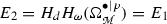
The above discussion can be related to the other spectral sequence which arises from the double complex having $\omega$ and d as differential, namely the one starting with d instead of $\omega$. In order to distinguish the two spectral sequences, we denote $E^d$ the one having d as vertical differential and $E^\omega$ the one having $\omega$ as vertical differential. By recalling that $\omega$ is d-exact, it is not hard to see that $E^d$ converges already at page 1 so that . In particular, one finds that for any $p = 1, \ldots , n$, so that the two spectral sequences converge indeed to the same space, isomorphic to n copies of ${\mathbb {R}}$, whereas all the pictures are taken into account. With reference to the cohomology of d, the non-trivial classes are generated (over ${\mathbb {R}}$) by the elements $\sum _{i_j} \theta _{i_1} \ldots \theta _{i_p} \delta (\hbox {d}\theta _{i_1}) \ldots \delta (\hbox {d}\theta _{i_p})$ for $i_j= 1, \ldots , n$, $p=0, \ldots , n$ and $i_j \ne i_k$, where the case $p=0$ corresponds indeed to the representative 1. Notice that here, just like in the cohomology of $\omega$ above, we might have chosen a single element instead of the sum above as a representative of for all $0<p<n$, since all of the elements in the sum are actually cohomologous—this fact can be proved in exactly the same way as we have done in “Appendix” for the cohomology of $\omega$; nonetheless, this more “democratic” choice looks the most suitable to us. Notice that all the classes in can be obtained from 1 upon using the picture raising operators related to d, i.e. ${\mathbb {Y}}^d$, whose definition is recalled in Sect. 4. Moreover, something which is really worth stressing is that the de Rham cohomology above contains an element which is also present in discussed above, namely the only element coming from the complex of integral forms at picture $p=n$, i.e. $\theta _1 \ldots \theta _n \delta (\hbox {d}\theta _1) \ldots \delta (\hbox {d}\theta _n):$ this will prove useful in what follows.

Finally, we address the relation between the (isomorphic) convergence spaces of the two spectral sequences, namely and . It is indeed possible to find an explicit map, carrying the representatives of one space to the other. For a generic element let us define the following integral transformation

$$\begin{aligned}&({\mathcal {F}}^\mathrm{odd} f) (x, \theta , \hbox {d}x , \hbox {d}\theta ) \nonumber \\&\quad {:}{=}\int [\hbox {d}\eta ^1 \ldots \hbox {d}\eta ^n | \hbox {d} \xi _1 \ldots \hbox {d} \xi _n] e^{\left( \sum _{i=1}^n \eta ^i \theta _i + \sum _{j=1}^n \xi _j \hbox {d}x^j \right) } f (x, \xi , \eta , \hbox {d}\theta ) \end{aligned}$$

(5.23)

where the symbol $[\hbox {d}\eta _1 \ldots \hbox {d}\eta _n | \hbox {d} \xi _1 \ldots \hbox {d} \xi _n]$ indicates that we are Berezin-integrating along the odd coordinates $\eta$’s and the $\xi$’s, i.e. along all the odd “coordinates”. The $\eta$’s and the $\xi$’s are paired with their natural duals, the $\theta$’s and the $\hbox {d}x$’s: here, it is worth remembering that we have identified $\theta _i = \partial _{\hbox {d}x^i}$, hopefully clarifying this duality. Also, notice that in the case of odd symplectic supermanifolds the symbol $[\hbox {d}\eta _1 \ldots \hbox {d}\eta _n | d\xi _1 \ldots d\xi _n]$ is invariant, so that the above is well defined.

Let us now consider the action of the integral transform ${\mathcal {F}}^\mathrm{odd}$ on a generic representative of the cohomology . We set $\omega (x, \theta , \hbox {d}x, \hbox {d}\theta ) = \theta _{i_1} \ldots \theta _{i_p} \delta (\hbox {d}\theta _{i_1}) \ldots \delta (\hbox {d}\theta _{i_p})$ and we compute

$$\begin{aligned}&( {\mathcal {F}}^\mathrm{odd} \omega ) (x, \theta , \hbox {d}x, \hbox {d}\theta ) \nonumber \\&\quad = \int [d^n\eta | d^n \xi ] e^{\left( \sum _{i=1}^n \eta ^i \theta _i + \sum _{j=1}^n \xi _j \hbox {d}x^j \right) } \xi _{i_1} \ldots \xi _{i_p} \delta (\hbox {d}\theta _{i_1}) \ldots \delta (\hbox {d}\theta _{i_p}). \end{aligned}$$

(5.24)

The integral can be factorized into two Berezin integrals,

$$\begin{aligned}&( {\mathcal {F}}^\mathrm{odd} \omega ) (x, \theta , \hbox {d}x, \hbox {d}\theta )\nonumber \\&\quad = \left( \int [d^n\eta ] e^{\sum _{i=1}^n {\eta ^i \theta _i}} \right) \left( \int [d^n\xi ] e^{\sum _{j=1}^n \xi _j \hbox {d}x^j } \xi _{i_1} \ldots \xi _{i_p} \right) \delta (\hbox {d}\theta _{i_1}) \ldots \delta (\hbox {d}\theta _{i_p}) \nonumber \\&\quad = \theta _1 \ldots \theta _n \left( \int [d^n\xi ] e^{\sum _{j=1}^n \xi _j \hbox {d}x^j } \xi _{i_1} \ldots \xi _{i_p} \right) \delta (\hbox {d}\theta _{i_1}) \ldots \delta (\hbox {d}\theta _{i_p}) \end{aligned}$$

(5.25)

The second integral yields

$$\begin{aligned} \int [d^n\xi ] e^{\sum _{j=1}^n \xi _j \hbox {d}x^j } \xi _{i_1} \ldots \xi _{i_p} = \hbox {d}x^{i_{p+1}} \ldots \hbox {d}x^{i_n}. \end{aligned}$$

(5.26)

Putting all of the pieces back together, one gets that

(5.27)

The inverse map is easily figured out as the anti-transform of the previous, and it maps to .

We show that it is easier to relate these cohomologies by using both the sets of PCO’s for d and for $\omega$ defined previously. As observed above, a hint comes from the fact that the element

$$\begin{aligned} \beta = c \cdot \theta _1 \ldots \theta _n \cdot \delta \left( d \theta _1 \right) \ldots \delta \left( \hbox {d} \theta _n \right) , \quad c \in {\mathbb {R}} \ . \end{aligned}$$

(5.28)

belongs to both of the cohomologies and : one can then use this elements as “pivot” and acts on it with the picture changing operators of d and $\omega$ as to get any elements of both the cohomologies. In particular, any representative in can be obtained by applying certain powers of the picture lowering operator ${\mathbb {Z}}^{\omega }$ to $\beta$:

$$\begin{aligned} c \cdot \theta _1 \ldots \theta _n \cdot \alpha ^{(n-k|k)} = \left[ \prod _{i=1}^{n-k} {\mathbb {Z}}^{\omega } \right] \beta \ \Longleftrightarrow \ \beta = \left[ \prod _{i=1}^{n-k} {\mathbb {Y}}^{\omega } \right] c \cdot \theta _1 \ldots \theta _n \cdot \alpha ^{(n-k|k)} \ . \end{aligned}$$

(5.29)

Analogously, any representative found in can be obtained by applying certain powers of the picture lowering operator ${\mathbb {Z}}^{d}$ to $\beta$:

$$\begin{aligned} c \cdot \alpha ^{(0|k)} = \left[ \prod _{i=1}^{n-k} {\mathbb {Z}}^{d} \right] \beta \ \Longleftrightarrow \ \beta = \left[ \prod _{i=1}^{n-k} {\mathbb {Y}}^{d} \right] c \cdot \alpha ^{(0|k)} \ . \end{aligned}$$

(5.30)

By confronting (5.29) and (5.30), we get the identity

$$\begin{aligned} \left[ \prod _{i=1}^{n-k} {\mathbb {Y}}^{\omega } \right] c \cdot \theta _1 \ldots \theta _n \cdot \alpha ^{(n-k|k)} = \left[ \prod _{i=1}^{n-k} {\mathbb {Y}}^{d} \right] c \cdot \alpha ^{(0|k)} \ , \end{aligned}$$

(5.31)

or analogously

$$\begin{aligned} c \cdot \theta _1 \ldots \theta _n \cdot \alpha ^{(n-k|k)}&= \left[ \prod _{i=1}^{n-k} {\mathbb {Z}}^{\omega } {\mathbb {Y}}^{d} \right] c \cdot \alpha ^{(0|k)}, \qquad \nonumber \\ c \cdot \alpha ^{(0|k)}&= \left[ \prod _{i=1}^{n-k} {\mathbb {Z}}^{d} {\mathbb {Y}}^{\omega } \right] c \cdot \theta _1 \ldots \theta _n \cdot \alpha ^{(n-k|k)} \ . \end{aligned}$$

(5.32)

We can evaluate explicitly these expression, thus obtaining the simple equations

$$\begin{aligned} c \cdot \theta _1 \ldots \theta _n \cdot \alpha ^{(n-k|k)}&= \left[ \prod _{i=1}^{n-k} \theta _{a_i} \hbox {d}x^{a_i} \right] c \cdot \alpha ^{(0|k)}, \qquad \nonumber \\ c \cdot \alpha ^{(0|k)}&= \left[ \prod _{i=1}^{n-k} \partial ^{a_i} \iota _{a_i} \right] c \cdot \theta _1 \ldots \theta _n \cdot \alpha ^{(n-k|k)} \ . \end{aligned}$$

(5.33)

This leads to the following interpretation: we can use the PCO’s as “ladder operators” in order to move from representatives of the cohomology of d to representatives of the cohomology of $\Delta _{BV}$ and vice versa, once again establishing an isomorphism between the two cohomologies, as the following diagram explains pictorially

(5.34)

We recollect the result of this section in the following theorem, which is in some sense the completion of Theorem 3.1.

Theorem 5.1

(BV cohomology and de Rham cohomology) Let be an odd symplectic supermanifold of dimension n|n and let for $p = 0, \ldots n$ be its extended de Rham double complex, let $E_\bullet ^\omega$ and $E_\bullet ^d$ be the spectral sequences starting with $\omega$ and d, respectively. Then the following are true.

• (1) for $p=0, \ldots , n$. This cohomology is generated over the real numbers by $[\theta _1 \ldots \theta _n \cdot \alpha _p]$ for $\alpha _{p}$ a generator of , as in Theorem 3.1, and it is isomorphic to ${\mathbb {R}}$ for any p. In particular, the homotopy of the BV operator $\Delta _{BV} {:}{=}\sum _{i=1}^n \partial _{x^i}\partial _{\theta _i}$ acting on local sections $f^I \theta _I$ of for some multi-index I is given by

  $$\begin{aligned} h (f^I \theta _I) {:}{=}\sum _{a=1}^n \left( \int _{0}^1 dt \,t^{Q_s} x^a G^{*}_t f^I (x)\right) \otimes \theta _a \theta _I, \end{aligned}$$

  (5.35)

  where $G^{*}_t f (x) = f(tx)$ for $t \in [0,1]$ and $Q_s = n-1 - \deg (\theta _I)$.

• (2) for $p=0,\ldots , n.$ This cohomology is generated over the real numbers by $[\sum _{i_j} \theta _{i_1} \ldots \theta _{i_p} \delta (d\theta _{i_1}) \ldots \delta (d\theta _{i_p})]$ for $i_j \ne i_k$, $p = 0, \ldots ,n$ and it is isomorphic to ${\mathbb {R}}$ for any p.

Finally, an explicit isomorphism between the cohomologies and is realized by using the PCO’s for $\omega$ and for d or via the map ${\mathcal {F}}^\mathrm{odd}$ in (5.23) and its inverse.

6 New PCO’s from old and analogies with Kodaira–Spencer-type theory

6.1 New picture changing operators from Old

In this section, we introduce new picture changing operators that are built starting from those described in Sect. 3. In particular, we define new odd picture changing operators, in contrast to those defined above. We will show that these new operators can be used to define the BV operator, but also different BV-type operators that changes the picture number as well. In particular, we define the operator $\displaystyle {\check{d}}$ via the picture changing operator ${\mathbb {Y}}^\omega$ that we have introduced above:

(6.1)

where we note that the operator ${\check{d}}$ raises the picture number by one, but it leaves the form degree invariant: in other words, it moves vertically in the “stack” of complexes in (2.1). Also, notice that this operator is nilpotent. In analogy, we define the operator $\displaystyle \hat{d}$ using ${\mathbb {Z}}^\omega$

(6.2)

Notice that ${\hat{d}}$ does not move vertically, but in oblique direction: it lowers the picture by one and raises the form degree by two.

Let us now recover the BV Laplacian introduced above, by means of ${\hat{d}}$ and ${\check{d}}$. Let us consider the operator

$$\begin{aligned} {\tilde{\Delta }} {:}{=}- \frac{1}{2} \left( {\check{d}} \circ \left( \omega \right) ^{-1} \circ \hat{d} + \hat{d} \circ \left( \omega \right) ^{-1} \circ {\check{d}} \right) \ , \end{aligned}$$

(6.3)

where $\omega$ is the odd symplectic form. We use the definitions of the operators in (6.1) and (6.2) to obtain, dropping the composition symbols

$$\begin{aligned} {\tilde{\Delta }}&= - \frac{1}{2} \Big [ \left( d {\mathbb {Y}}^{\omega } - {\mathbb {Y}}^{\omega } d \right) \left( \omega \right) ^{-1} \left( d {\mathbb {Z}}^{\omega } - {\mathbb {Z}}^{\omega } d \right) \nonumber \\&\quad + \left( d {\mathbb {Z}}^{\omega } - {\mathbb {Z}}^{\omega } d \right) \left( \omega \right) ^{-1} \left( d {\mathbb {Y}}^{\omega } - {\mathbb {Y}}^{\omega } d \right) \Big ] \ . \end{aligned}$$

(6.4)

When acting on the cohomology of $\omega$, i.e. taking an element , it is easy to show that only two terms are not trivial and the action is exactly that of the BV Laplacian:

$$\begin{aligned} {\tilde{\Delta }} \alpha = \frac{1}{2} \left[ {\mathbb {Y}}^{\omega } \Delta _{BV} {\mathbb {Z}}^{\omega } + {\mathbb {Z}}^{\omega } \Delta _{BV} {\mathbb {Y}}^{\omega } \right] \alpha = \Delta _{BV} \alpha . \end{aligned}$$

(6.5)

The interested reader can find in “Appendix” an explicit example, showing the action of (6.3).

Likewise, one can define “BV-type operators” which modify the picture and the form number:

$$\begin{aligned} \Delta _{BV}^{(-2|2)}&{:}{=}{\check{d}} \circ \omega ^{-1} \circ {\check{d}}, \end{aligned}$$

(6.6)

$$\begin{aligned} \Delta _{BV}^{(-1|1)}&{:}{=}\frac{1}{2} \left[ {\check{d}} \circ \omega ^{-1} \circ d + d \circ \omega ^{-1} \circ {\check{d}} \right] , \end{aligned}$$

(6.7)

$$\begin{aligned} \Delta _{BV}^{(1|-1)}&{:}{=}\frac{1}{2} \left[ \hat{d} \circ \omega ^{-1} \circ d + d \circ \omega ^{-1} \circ \hat{d} \right] , \end{aligned}$$

(6.8)

$$\begin{aligned} \Delta _{BV}^{(2|-2)}&{:}{=}\hat{d} \circ \omega ^{-1} \circ \hat{d}. \end{aligned}$$

(6.9)

Again, the action of these operators can be obtained from $\Delta _{BV}$ and the two PCO’s $\displaystyle {\mathbb {Y}}^{\omega }$ and ${\mathbb {Z}}^{\omega }$, as above.

6.2 Analogies with Kodaira–Spencer-type theory and deformations

In this section, we describe an analogy with complex geometry which makes use of the picture changing operators introduced in the previous sections.

We start recalling basic facts about almost complex structures. Given a real manifold ${M}^{2n}$ of dimension 2n, an almost complex structure is an endomorphism of tangent space ${\mathcal {J}} \in End ({\mathcal {T}}{M^{2n}})$ such that ${\mathcal {J}}^2 = -\text {id}_{{\mathcal {T}}{M^{2n}}}$. Locally one can represent ${\mathcal {J}}$ as a sum ${\mathcal {J}} = J + {\bar{J}}$, with

$$\begin{aligned} \ J {:}{=}J^b_{{\bar{a}}} d {\bar{z}}^{{\bar{a}}} \otimes \partial _b, \qquad {\bar{J}} {:}{=}{\bar{J}}^{{\bar{b}}}_a dz^a \otimes {\bar{\partial }}_{{\bar{b}}} \end{aligned}$$

(6.10)

such that $J^a_{{\bar{a}}} {\bar{J}}^{{\bar{a}}}_b = - \delta ^a_b$ and $J^a_{{\bar{a}}} {\bar{J}}^{{\bar{b}}}_a = - \delta _{{\bar{a}}}^{{\bar{b}}}$. In particular, these can be used to transform holomorphic vectors into anti-holomorphic vectors and vice versa:

$$\begin{aligned} J \left( {\bar{\partial }}_{{\bar{a}}} \otimes 1 \right) = \left( J^b_{{\bar{c}}} d {\bar{z}}^{{\bar{c}}} ( {\bar{\partial }}_{{\bar{a}}} ) \right) \partial _b = J^b_{{\bar{a}}} \partial _b \ , \ {\bar{J}} \left( \partial _a \otimes 1 \right) = \big ( {\bar{J}}^{{\bar{b}}}_c dz^c \left( \partial _a \right) \big ) {\bar{\partial }}_{{\bar{b}}} = {\bar{J}}^{{\bar{b}}}_a {\bar{\partial }}_{{\bar{b}}} \ . \end{aligned}$$

(6.11)

Analogously, one can use J and ${{\bar{J}}}$ to take holomorphic (1, 0)-forms into anti-holomorphic (0, 1)-forms and vice versa, upon using that $({\mathcal {T}}^*M^{2n})^*\cong {\mathcal {T}} M^{2n}:$

$$\begin{aligned} J \left( 1 \otimes d z^a \right)= & {} J^b_{{\bar{a}}} d {\bar{z}}^{{\bar{a}}} \otimes \partial _b \left( dz^a \right) = J^a_{{\bar{a}}} d {\bar{z}}^{{\bar{a}}} \ , \nonumber \\ \ {\bar{J}} \left( 1 \otimes d {\bar{z}}^{{\bar{a}}} \right)= & {} {\bar{J}}^{{\bar{b}}}_a dz^a \otimes {\bar{\partial }}_{{\bar{b}}} \left( d {\bar{z}}^{{\bar{a}}} \right) = {\bar{J}}^{{\bar{a}}}_a dz^a \ . \end{aligned}$$

(6.12)

In the previous formulae, one can rewrite J and ${{\bar{J}}}$ as

$$\begin{aligned} J = J^b_{{\bar{a}}} d {\bar{z}}^{{\bar{a}}} \iota _b, \qquad {\bar{J}} = {\bar{J}}^{{\bar{b}}}_a dz^a {\bar{\iota }}_{{\bar{b}}} \ , \end{aligned}$$

(6.13)

where $\iota _a$ and ${\bar{\iota }}_{{\bar{a}}}$ are the contractions along a holomorphic and a anti-holomorphic base vector, respectively.

By using the almost complex structure, we can define the Nijehuis tensor N:

$$\begin{aligned} N \left( U , V \right) = \left[ J (U) , J (V) \right] - J \left[ J (U) , V \right] - J \left[ U , J (V) \right] - \left[ U , V \right] \end{aligned}$$

(6.14)

where $U, V \in {\mathcal {T}}M^{2n}$. The vanishing of N is said integrability condition: an almost complex structure with vanishing N defines a complex structure so that the pair $(M^{2n}, {\mathcal {J}})$ lifts to a complex manifold X. Remarkably, integrability of N is equivalent to nilpotency of the anti-Dolbeault operator:

$$\begin{aligned} N = 0 \ \Longleftrightarrow \ {\bar{\partial }}^2 = 0. \end{aligned}$$

(6.15)

Taking this point of view, for a certain complex manifold X, given a (0, 1)-form valued in ${\mathcal {T}}_X$, call it $A \in \Omega ^{(0,1)}_X \otimes {\mathcal {T}}_X$, the deformations of the complex structure of X are therefore defined by the equation $({{\bar{\partial }}} + A)^2 = 0$, that is

$$\begin{aligned} {\bar{\partial }} A + A \wedge A = 0. \end{aligned}$$

(6.16)

Writing $A= d {\bar{z}}^{{\bar{i}}} A_{{\bar{i}}}^j \partial _j$, this reads

$$\begin{aligned} {\bar{\partial }}A^i + A^j \partial _j A^i = 0, \end{aligned}$$

(6.17)

which is the Tian–Todorov equation for the deformations of complex structures, see [19].

We now try to make a connection with the construction of the previous section: we argue the following analogy

$$\begin{aligned} \text{ holomorphic } \text{ forms } \quad&\longleftrightarrow \quad \hbox {d}x^i, \end{aligned}$$

(6.18)

$$\begin{aligned} \text{ anti-holomorphic } \text{ forms } \quad&\longleftrightarrow \quad \delta (\hbox {d}\theta _i). \end{aligned}$$

(6.19)

In other words, we identify the form degree with the holomorphic form degree and the picture number with the anti-holomorphic form degree in a theory over the complex numbers—notice that the $\delta (\hbox {d}\theta )$’s transform (at first order) exactly as a form on the underlying manifold. First, let us see how the analogue of a complex structure looks like. Using the above analogy, from (6.13), we see that J and ${\bar{J}}$ become a sort of non-diagonal versions of the previously introduced picture changing operators. In particular, along with this analogy, one can introduce a new picture raising operator, namely

$$\begin{aligned} \check{{\mathbb {Y}}} {:}{=}J^i_j \delta \left( \hbox {d} \theta _j \right) \iota _i, \end{aligned}$$

(6.20)

which can also be rewritten as $\check{{\mathbb {Y}}} = J^i_j \delta \left( \hbox {d} \theta _j \right) \otimes \partial _i,$ upon using the natural isomorphism In particular, using this representation, we can define the action of (6.20) on vector fields:

$$\begin{aligned} \check{{\mathbb {Y}}} \left( \partial ^i \otimes 1 \right)&= J^j_k \left[ \delta \left( \hbox {d} \theta _k \right) \left( \partial ^i \right) \right] \partial _j = J^j_k \left[ \delta \left( \iota ^i \right) \delta \left( \hbox {d} \theta _k \right) \right] \partial _j = J^j_k \delta ^k_i \partial _j = J^j_i \partial _j \ , \end{aligned}$$

(6.21)

$$\begin{aligned} \check{{\mathbb {Y}}} \left( \partial _i \otimes 1 \right)&= 0 \ . \end{aligned}$$

(6.22)

where $\delta (\iota ^i)$ is defined by its Fourier representation, see, for example, [41]. Similarly, the picture lowering operator reads

$$\begin{aligned} \check{{\mathbb {Z}}} = J^i_j \hbox {d}x^j \delta \left( \iota ^i \right) , \end{aligned}$$

(6.23)

Given these definitions, we can construct the analogous of the Nijenhuis tensor (6.14) above, but taking $J {:}{=}\check{{\mathbb {Z}}} + \check{{\mathbb {Y}}}$ and where the brackets are now graded. In particular, let us consider the action of this tensor, we call it ${\check{N}}$, on two odd coordinate fields—notice that it follows from (6.22) that on even coordinate fields it yields zero. It can be seen that

$$\begin{aligned} {\check{N}} \left( \partial ^i , \partial ^j \right) = \left[ {\mathbb {Y}} (\partial ^i) , {\mathbb {Y}} (\partial ^j) \right] = \left( J_i^k \partial _k J^l_j - J_j ^k \partial _k J^l_i \right) \partial _l \ . \end{aligned}$$

(6.24)

Let us consider the case ${\check{N}} \left( \partial ^i , \partial ^j \right) = 0$, which can be seen as the analogue condition $N (U,V) = 0$ when applied to two anti-holomorphic coordinate base vectors. It is remarkable to observe that in analogy with (6.15) we find that

$$\begin{aligned} {\check{d}}^2 = 0 \ \Longleftrightarrow \ \delta \left( \hbox {d} \theta _i \right) \delta \left( \hbox {d} \theta _j \right) J_i^k \partial _k J^l_j \partial _l = 0 \ \Longleftrightarrow \ \left( J_i^k \partial _k J^l_j - J_j^k \partial _k J^\rho _i \right) \partial _l = 0 \ , \end{aligned}$$

(6.25)

where the anti-symmetrization is due to $\delta \left( \hbox {d} \theta \right)$ being odd. In other words, the requirement of nilpotency of the operator ${\check{d}}$ is analogous to the requirement of vanishing of ${\check{N}}$ along odd directions (along even directions is automatic). We can push forward our analogy to make contact with deformations of complex structure. In this context, we consider in particular Kodaira–Spencer theory [7] which accounts for the deformations of the complex structure of a certain Calabi–Yau threefold $CY_3$.

First of all, it is worth observing that one can deform the equation above ${\check{d}}^2 = 0$ by setting ${\check{d}} \mapsto {\check{d}} + \delta \left( \hbox {d} \theta _i \right) A_i^j \partial _j = {\check{d}} + \delta A^j \partial _j$ as to get the equation

$$\begin{aligned} {\check{d}} A^i + A^j \partial _j A^i = 0 \ , \end{aligned}$$

(6.26)

which has the same form as Eq. (6.17). Moreover, it is possible to obtain this equation from a field theory action, in analogy with the Kodaira–Spencer action, that we briefly recall. Given a Calabi–Yau threefold $CY_3$, the action reads

$$\begin{aligned} S = \int _{CY_3} A' \wedge \frac{1}{\partial } {\bar{\partial }} A'+ A' \wedge \left( A \wedge A \right) ' \ , \end{aligned}$$

(6.27)

where $\displaystyle A\in \Omega ^{(0,1)}_{CY_3} \otimes T^{(1,0)}_{CY_3}$, see [7] for details. The prime appearing above amounts to the map $A \mapsto A \wedge \Omega$, where $\Omega$ is the (global) holomorphic 3-form of $CY_3,$ that is

$$\begin{aligned} A^\prime = \left( d {\bar{z}}^{{\bar{i}}} A_{{\bar{i}}}^j \partial _j \right) \left( \Omega _{r k l} d z^r \wedge d z^k \wedge d z^l \right) = A_{{\bar{i}}}^j \Omega _{j k l} d {\bar{z}}^{{\bar{i}}} \wedge d z^k \wedge d z^l \in \Omega _{CY_3}^{(2,1)}. \end{aligned}$$

(6.28)

As already said, the variation of the action leads to the Tian–Todorov equation (6.17).

Let us exploit the analogy described above to deduce the action leading to (6.26). In particular, instead of the field A, we consider the picture changing operator $\check{{\mathbb {Y}}} = \delta \left( \hbox {d} \theta _i \right) J_i^j \iota _j$. The map via the holomorphic 3-form described above now amounts to apply the operator $\check{{\mathbb {Y}}}$ to the volume form $\epsilon _{i j k}\hbox {d}x^i \wedge \hbox {d}x^j \wedge \hbox {d}x^k$ of the reduced manifold, hence

$$\begin{aligned} \left( \check{{\mathbb {Y}}} \right) ^\prime = \delta \left( \hbox {d} \theta _i \right) J_i^j \epsilon _{j k l} \hbox {d}x^k \wedge \hbox {d}x^l \ . \end{aligned}$$

(6.29)

In analogy with the Kodaira–Spencer action, one therefore writes

(6.30)

where is a supermanifold of dimension 3|3. The equations of motion read

$$\begin{aligned} {\check{d}} \left( \check{{\mathbb {Y}}} \right) '+ d \left( \check{{\mathbb {Y}}} \wedge \check{{\mathbb {Y}}} \right) ' = 0, \end{aligned}$$

(6.31)

which, in turn, performing the calculations, yield

$$\begin{aligned} \partial _{[i} J^j_{k]} + \partial _l J^j_{[i} J_{k]}^l = 0. \end{aligned}$$

(6.32)

These are the analogous of the Tian–Todorov equations.

Appendix A. Cohomology and Transformation Properties for \(n=2\)

In this appendix, we aim at clarifying the constructions of the previous section in the easy but non-trivial case $n=2$.

Let us start from the cohomology of $\omega$: while the cases of differential and integral forms are trivial, the case of pseudo-forms deserves some more attention. First let us show that the representatives $\hbox {d}x^1 \delta (\mathrm{d}\theta _2)$ and $-\hbox {d}x^2 \delta (\mathrm{d}\theta _1)$ in are cohomologous. Let $t \in [0,1]$, consider the following family

$$\begin{aligned} \phi _t {:}{=}\left( \left( 1 - t \right) \hbox {d}x^1 - t \hbox {d}x^2 \right) \delta \left( t \hbox {d} \theta _1 + \left( 1-t \right) \hbox {d} \theta _2 \right) . \end{aligned}$$

(A.1)

Notice that $\phi _0 = \hbox {d}x^{1} \delta (\mathrm{d}\theta _2)$ and $\phi _1 = -\hbox {d}x^2 \delta (\mathrm{d}\theta _1)$. A short calculation yields that for any $t \in [0,1]$ one has that $\omega \phi _t =0,$ i.e. $\phi _t$ is closed for any t. Also, upon using the properties of the delta’s, one finds

$$\begin{aligned} \phi _t&= \hbox {d}x^1 \delta \left( \hbox {d} \theta _2 + \frac{t}{1-t} \hbox {d} \theta _1 \right) - \frac{t}{1-t} \hbox {d}x^2 \delta \left( \hbox {d} \theta _2 + \frac{t}{1-t} \hbox {d} \theta _1 \right) \nonumber \\&= \hbox {d}x^1 \delta \left( \hbox {d} \theta _2 \right) + \sum _{n=1}^{\infty } \hbox {d}x^1 \frac{1}{n!} \left( \frac{t}{1-t} \right) ^n \hbox {d} \theta _1^n \delta ^{(n)} \left( \hbox {d} \theta _2 \right) \nonumber \\&\quad - \sum _{n=0}^\infty \hbox {d}x^2 \frac{1}{n!} \left( \frac{t}{1-t} \right) ^{n+1} \hbox {d} \theta _1^n \delta ^{(n)} \left( \hbox {d} \theta _2 \right) . \end{aligned}$$

(A.2)

The second and third terms gather in an exact term as to give

$$\begin{aligned} \phi _t = \hbox {d}x^1 \delta \left( \hbox {d} \theta _2 \right) + \omega \left( \sum _{n=1}^{\infty } \frac{1}{n!} \left( \frac{t}{1-t} \right) ^n d \theta _1^{n-1} \delta ^{(n)} \left( \hbox {d} \theta _2 \right) \right) . \end{aligned}$$

(A.3)

Hence, $\phi _t \equiv \hbox {d}x^1 \delta (\mathrm{d}\theta _2)\, \text{ mod } (\omega ).$ Likewise, one sees that

$$\begin{aligned} \phi _t = -\hbox {d}x^2 \delta \left( \hbox {d} \theta _1 \right) - \omega \left( \sum _{n=1}^{\infty } \frac{1}{n!} \left( \frac{1-t}{t} \right) ^n d \theta _2^{n-1} \delta ^{(n)} \left( \hbox {d} \theta _1 \right) \right) , \end{aligned}$$

(A.4)

that is $\phi _t \equiv -\hbox {d}x^2 \delta (\mathrm{d}\theta _1)\, \text{ mod } (\omega ),$ so that in turn $\phi _0 = \hbox {d}x^1 \delta (\mathrm{d}\theta _2) \sim \phi _t \sim - \hbox {d}x^2 \delta (\mathrm{d}\theta _1) = \phi _1,$ thus showing that the two elements are indeed cohomologous.

On the same line, this result could have been obtained also by observing that if we write a generic cohomology representative of by choosing a certain vector V, singling out a certain direction, $\alpha ^{1|1}_V = V^i \epsilon _{ij} \hbox {d}x^j \delta ( V^i \mathrm{d}\theta _i),$ then it is not hard to show that the infinitesimal variation of $\alpha ^{1|1}_V$ with respect to V reads $\delta \alpha ^{1|1}_V = \omega \left( V^i \epsilon _{i j} \delta V^j \delta ^{(1)}( V^i \mathrm{d}\theta _i) \right)$. This says that the dependence on the choice of the vector V is $\omega$-exact and the cohomology representative is unique.

Let us now address the transformation properties of the representatives in the cohomology at picture $p=1$ and show that they indeed transforms as semidensities over Let us consider a certain change of coordinates of . By the transformation properties of an odd symplectic supermanifold discussed in the first section of this paper, the action on forms goes as follows

$$\begin{aligned} \left( \begin{matrix} \hbox {d}x^1 \\ \hbox {d}x^2 \\ \hbox {d} \theta _1 \\ \hbox {d} \theta _2 \end{matrix} \right) \longmapsto \left( \begin{matrix} a &{} \quad b &{} \quad 0 &{} \quad 0 \\ c &{} \quad d &{} \quad 0 &{} \quad 0 \\ 0 &{} \quad 0 &{} \quad \frac{d}{\Delta } &{} \quad -\frac{c}{\Delta } \\ 0 &{} \quad 0 &{} \quad -\frac{b}{\Delta } &{} \quad \frac{a}{\Delta } \end{matrix} \right) \left( \begin{matrix} \hbox {d}x^1 \\ \hbox {d}x^2 \\ \hbox {d} \theta _1 \\ \hbox {d} \theta _2 \end{matrix} \right) \ , \end{aligned}$$

(A.5)

where $\Delta = ad-bc$ is the determinant of the matrix A, which is nothing but the Jacobian of the change of coordinates on the reduced manifold Let us now consider the representative $\hbox {d}x^1 \delta (\mathrm{d}\theta _2)$, one finds (for $a \ne 0$)

$$\begin{aligned}&\hbox {d}x^1 \delta \left( \hbox {d} \theta _2 \right) \longmapsto \left( a \hbox {d}x^1 + b \hbox {d}x^2 \right) \delta \left( \frac{a}{\Delta } \hbox {d} \theta _2 - \frac{b}{\Delta } \hbox {d} \theta _1 \right) \nonumber \\&\quad = \Delta \left[ \hbox {d}x^1 \delta \left( \hbox {d} \theta _2 \right) + \sum _{n=1}^\infty \frac{\left( \hbox {d} \theta _1 \right) ^n }{n!} \left( - \frac{b}{a} \right) ^n \delta ^{(n)} \left( \hbox {d} \theta _2 \right) \right. \nonumber \\&\left. \qquad + \sum _{n=0}^\infty \frac{\left( \hbox {d} \theta _1 \right) ^n }{n!} \left( \frac{b}{a} \right) ^{n+1} \delta ^{(n)} \left( \hbox {d} \theta _2 \right) \right] \ , \end{aligned}$$

(A.6)

where we have expanded the $\delta$’s with respect to $\hbox {d} \theta _2$ and left the closed, non-exact term $\hbox {d}x^1 \delta \left( \hbox {d} \theta _2 \right)$ explicit. All the terms, except for the first, group together to form $\omega$-exact terms: in particular, one finds that

$$\begin{aligned} \hbox {d}x^1 \delta \left( \hbox {d} \theta _2 \right) \mapsto \Delta \hbox {d}x^1 \delta \left( \hbox {d} \theta _2 \right) + \omega \left( \Delta \sum _{n=1}^\infty \frac{1}{n!} \left( - \frac{b}{a} \right) ^n \left( \hbox {d} \theta _1 \right) ^{n-1} \delta ^{(n)} \left( \hbox {d} \theta _2 \right) \right) , \end{aligned}$$

(A.7)

which shows that $[\hbox {d}x^1 \delta (\hbox {d}\theta _2)] \mapsto \det (A) [\hbox {d}x^1 \delta (\hbox {d}\theta _2)]$ in cohomology, which concludes the proof.

Finally, we want to show the explicit calculations for the operator defined in (6.3). For the sake of clarity, let us consider the action of (6.3) on $\alpha = f(x,\theta ) \hbox {d}x^1 \hbox {d}x^2$ (we assume for simplicity that $|f| = 0$). We have

$$\begin{aligned} {\tilde{\Delta }} \alpha = - \frac{1}{2} \hat{d} \circ \omega ^{-1} \circ {\check{d}} \alpha \ , \end{aligned}$$

(A.8)

since $\hat{d} \alpha = 0$. Let us first calculate ${\check{d}}\alpha$:

$$\begin{aligned} {\check{d}} \alpha&= d \left[ - f \hbox {d}x^2 \delta \left( \hbox {d} \theta _1 \right) + f \hbox {d}x^1 \delta \left( \hbox {d} \theta _2 \right) \right] \\&\quad - {\mathbb {Y}}^{\omega } \left[ \partial ^1 f \hbox {d} \theta _1 \hbox {d}x^1 \hbox {d}x^2 + \partial ^2 f \hbox {d} \theta _2 \hbox {d}x^1 \hbox {d}x^2 \right] \\&= \omega \left[ \partial _1 f \hbox {d}x^2 \delta ' \left( d \theta _1 \right) - \partial _2 f \hbox {d}x^1 \delta ' \left( \hbox {d} \theta _2 \right) \right] . \end{aligned}$$

We are therefore left with

$$\begin{aligned} (\hat{d} \circ \omega ^{-1} \circ {\check{d}}) \alpha = \left( d {\mathbb {Z}}^{\omega } - {\mathbb {Z}}^{\omega } d \right) \left[ \partial _1 f \hbox {d}x^2 \delta ' \left( \hbox {d} \theta _1 \right) - \partial _2 f \hbox {d}x^1 \delta ' \left( \hbox {d} \theta _2 \right) \right] \ . \end{aligned}$$

(A.9)

Let us show that the first term is trivially 0. Indeed, by recalling the algebraic rules $\displaystyle -i \Theta \delta \left( \hbox {d} \theta \right) = {1}/{\hbox {d} \theta }$ and $\displaystyle -i \Theta \delta ' \left( \hbox {d} \theta \right) = - {1}/{(\hbox {d} \theta )^2}$, one has

$$\begin{aligned} {\mathbb {Z}}^{\omega } {\check{d}} \alpha&= -i \left( \omega \Theta + \Theta \omega \right) \left[ \partial _1 f \hbox {d}x^2 \delta ' \left( \hbox {d} \theta _1 \right) - \partial _2 f \hbox {d}x^1 \delta ' \left( \hbox {d} \theta _2 \right) \right] \end{aligned}$$

(A.10)

$$\begin{aligned}&= \partial _1 f \frac{\hbox {d}x^1 \hbox {d}x^2}{\hbox {d} \theta _1} + \partial _2 f \frac{\hbox {d}x^1 \hbox {d}x^2}{\hbox {d} \theta ^2} - \partial _1 f \frac{\hbox {d}x^1 \hbox {d}x^2}{\hbox {d} \theta _1} - \partial _2 f \frac{\hbox {d}x^1 \hbox {d}x^2}{d \theta _2} = 0 \ . \end{aligned}$$

(A.11)

We are therefore left with

$$\begin{aligned}&{\mathbb {Z}}^{\omega } d \left( \partial _1 f \hbox {d}x^2 \delta ' \left( \hbox {d} \theta _1 \right) - \partial _2 f \hbox {d}x^1 \delta ' \left( d \theta _2 \right) \right) \nonumber \\&\quad = {\mathbb {Z}}^{\omega } \left( - \partial ^1 \partial _1 f \hbox {d}x^2 \delta \left( \hbox {d} \theta _1 \right) + \partial ^2 \partial _2 f \hbox {d}x^1 \delta \left( \hbox {d} \theta _2 \right) \right) \ . \end{aligned}$$

(A.12)

It is useful to observe that the two terms in (A.12) are representatives of , hence they are $\omega$-closed: the previous equation thus reduces to

$$\begin{aligned}&-i \omega \Theta \left( - \partial ^1 \partial _1 f \hbox {d}x^2 \delta \left( \hbox {d} \theta _1 \right) + \partial ^2 \partial _2 f \hbox {d}x^1 \delta \left( d \theta _2 \right) \right) \nonumber \\&\quad = \omega \left( - \partial ^1 \partial _1 f \frac{\hbox {d}x^2}{\hbox {d} \theta _1} + \partial ^2 \partial _2 f \frac{\hbox {d}x^1}{d \theta _2} \right) \nonumber \\&\quad = \partial ^1 \partial _1 f \hbox {d}x^1 \hbox {d}x^2 + \partial ^2 \partial _2 f \hbox {d}x^1 \hbox {d}x^2 = \Delta _{BV} f \hbox {d}x^1 \hbox {d}x^2 \ , \end{aligned}$$

(A.13)

hence proving the claim.

References

Batalin, I.A., Vilkovisky, G.A.: Gauge algebra and quantization. Phys. Lett. B 102, 1 (1981)
Belopolsky, A.: Picture changing operators in supergeometry and superstring theory. arXiv:hep-th/9706033
Belopolsky, A.: New geometrical approach to superstrings. arXiv: hep-th/9703183 (1997)
Berkovits, N.: Multiloop amplitudes and vanishing theorems using the pure spinor formalism for the superstring. JHEP 0409, 047 (2004)
Bernstein, J., Leites, D.: Integral forms and Stokes formula on supermanifolds. Funct. Anal. Appl. 11(1), 55–56 (1977)
Bernstein, J., Leites, D.: How to integrate differential forms on supermanifolds. Funct. Anal. Appl. 11(3), 70–71 (1977)
Bershadsky, M., Cecotti, S., Ooguri, H., Vafa, C.: Kodaira–Spencer theory of gravity and exact results for quantum string amplitudes. Commun. Math. Phys. 165, 311–427 (1994)
Cacciatori, S.L., Noja, S.: Projective superspaces in practice. J. Geom. Phys. 130, 40–62 (2018)
Cacciatori, S., Noja, S., Re, R.: Non projected Calabi–Yau supermanifolds over \({\mathbb{P}}^2\). Math. Res. Lett. 26(4), 1027–1058 (2019)
Cacciatori, S.L., Noja, S., Re, R.: The unifying double complex on supermanifolds. arXiv: 2004.10906
Carmeli, C., Caston, L., Fioresi, R.: Mathematical foundations of supersymmetry. EMS (2011)
Castellani, L., Catenacci, R., Grassi, P.A.: Integral representations on supermanifolds: super hodge duals, PCOs and Liouville forms. Lett. Math. Phys. 107(1), 167 (2017)
Catenacci, R., Grassi, P.A., Noja, S.: Superstring field theory, superforms and supergeometry. J. Geom. Phys. 148, 103559 (2020)
Catenacci, R., Grassi, P.A., Noja, S.: \(A_\infty \)-Algebra from supermanifolds. Ann. Henri Poincaré 20(12), 4163–4195 (2019)
Cremonini, C.A., Grassi, P.A.: Pictures from Super Chern–Simons theory. JHEP 2003, 043 (2020)
Cremonini, C.A., Grassi, P.A.: Super Chern–Simons theory: BV-formalism and \(A_\infty \)-algebras. arXiv:1912.10807
Cremonini, C.A., Grassi, P.A., Penati, S.: Supersymmetric Wilson loops via integral forms. arXiv:2003.01729
Friedan, D., Martinec, E., Shenker, S.: Conformal invariance, supersymmetry and string theory. Nucl. Phys. B 271, 93 (1986)
Hori, K., et al.: Mirror Symmetry, Clay Mathematical Monograph. AMS (2003)
Khudaverdian, H.M.: Semidensities on odd symplectic supermanifolds. Commun. Math. Phys. 247, 353–390 (2004)
Khudaverdian, H.M.: Laplacians in odd symplectic geometry. Contemp. Math. 315, 199–212 (2002)
Khudaverdian, H.M., Voronov, T.T.: Differential forms and odd symplectic geometry. In: Buchstaber, V.M., Krichever, I.M. (eds.) Geometry, Topology and Mathematical Physics. S. P. Novikov seminar: 2006–2007 AMS Translations, Series 2, vol. 224, pp. 159–171. American Mathematical Society, Providence (2008)
Khudaverdian, H.M.: Geometry of superspace with even and odd brackets. J. Math. Phys. 32, 1938–1941 (1991)
Khudaverdian, H.M.: Odd invariant semidenstiy and divergence-like operators on odd symplectic superspace. Commun. Math. Phys. 198, 591–606 (1998)
Manin, Y.I.: Gauge Field Theory And Complex Geometry. Springer, New York (1988)
Mnev, P.: Quantum Field Theory: Batalin–Vilkovisky Formalism and its Applications. AMS, London (2019)
Noja, S., Cacciatori, S.L., Dalla Piazza, F., Marrani, A., Re, R.: One-dimensional super Calabi–Yau manifolds and their mirrors. JHEP 1704, 094 (2017)
Noja, S.: Non-Projected Supermanifolds and Embeddings in Super Grassmannians, Universe, vol 4, no. 11, p. 114 (2018). Special Issue “Super Geometry for Super Strings”
Noja, S.: Supergeometry of \(\Pi \)-projective spaces. J. Geom. Phys. 124, 286–299 (2018)
Noja, S., Re, R.: A Note on super Koszul complex and the Berezinian. ArXiv:2012.02739
Ogievetskii, O.V., Penkov, I.B.: Serre duality for projective supermanifolds. Funct. Anal. its Appl. 18, 68–70 (1984)
Penkov, I.B.: \({\mathscr {D}}\)-modules on supermanifolds. Invent. Math. 71, 501–512 (1983)
Ševera, P.: On the origin of the BV operator on odd symplectic supermanifolds. Lett. Math. Phys. 78, 55–59 (2006)
Schwarz, A.S.: Geometry of Batalin–Vilkovisky quantization. Commun. Math. Phys. 155, 249–260 (1993)
Voronov, T., Zorich, A.: Complexes of forms on a supermanifold. Funct. Anal. Appl. 20(2), 58–59 (1986)
Voronov, T., Zorich, A.: Integral transformations of pseudodifferential forms. Russ. Math. Surv. 41(6), 221–222 (1986)
Voronov, T., Zorich, A.: Integration on vector bundles. Funct. Anal. Appl. 22(2), 94 103 (1988)
Voronov, T.: Supermanifold forms and integration. A dual theory, In: Solitons, Geometry, and Topology: On the Crossroad, AMS Translations, Series, vol. 2, no. 179, Providence, RI, pp. 153–172 (1997)
Voronov, T.T.: Geometric Integration Theory on Supermanifolds. Cambridge Scientific Publisher, Cambridge (2014)
Voronov, T.: Dual forms on supermanifolds and Cartan calculus. Commun. Math. Phys. 228, 1–16 (2002)
Witten, E.: Notes on supermanifolds and integration. Pure Appl. Math. Q. 15(1), 3–56 (2019)
Acknowledgements
We thank the anonymous referees for important remarks about the manuscript. This work has been partially supported by Università del Piemonte Orientale research funds, by Italian Ministero dell’Università e della Ricerca (MIUR) and by Istituto Nazionale di Fisica Nucleare (INFN) through the “FieLds And Gravity” (FLAG) and “Gauge theories, Strings, Supergravity” (GSS) research projects.
Funding
Open access funding provided by Universitá degli Studi del Piemonte Orientale Amedeo Avogrado within the CRUI-CARE Agreement.
Author information
Authors and Affiliations
Corresponding author
Additional information
Publisher's Note
Springer Nature remains neutral with regard to jurisdictional claims in published maps and institutional affiliations.