Detecting concept change in dynamic data streams

Abstract

In this research we present a novel approach to the concept change detection problem. Change detection is a fundamental issue with data stream mining as classification models generated need to be updated when significant changes in the underlying data distribution occur. A number of change detection approaches have been proposed but they all suffer from limitations with respect to one or more key performance factors such as high computational complexity, poor sensitivity to gradual change, or the opposite problem of high false positive rate. Our approach uses reservoir sampling to build a sequential change detection model that offers statistically sound guarantees on false positive and false negative rates but has much smaller computational complexity than the ADWIN concept drift detector. Extensive experimentation on a wide variety of datasets reveals that the scheme also has a smaller false detection rate while maintaining a competitive true detection rate to ADWIN.

1 Introduction

Data stream mining has been the subject of extensive research over the last decade or so. The well known CVFDT (Hulten et al. 2001) algorithm is a good example of an early algorithm that proposed an incremental approach to building and maintaining a decision tree in the face of changes or concept drift that occur in a data stream environment. Since then there has a multitude of refinements to CVFDT, CBDT (Hoeglinger and Pears 2007; Hoeglinger et al. 2009) and to other methods (Widiputra et al. 2011) that perform other types of mining such as a clustering and prediction on data streams. The fundamental issue with data stream mining is to manage the sheer volume of data which grows continuously over time. A closely connected problem is adaptation of models to changes that take place in the stream. In this respect concept change detection is a crucial issue as it enables models to replace outdated concepts with current concepts.

Concept change detection has been studied extensively by both the statistical and machine learning communities. The main incentive within the statistical community has been in the manufacturing and process control applications, whereby changes in equipment due to wear and tear over time can cause changes in the quality of products. The machine learning community has a different interest: whether models induced from historical data perform equally well on newly arriving data or whether performance has degraded due to changes in the underlying data distribution. In a data stream environment, data arrives on a continuous basis and concept drift causes changes in patterns, thus requiring models to be changed on an ongoing basis and hence a need arises for the automation of the concept change detection process. The methods proposed for concept change detection all tend to suffer from limitations with respect to one or more key performance factors such as high computational complexity, poor sensitivity to gradual change or drift, or the opposite problem of high false positive rate. In this research we propose a novel sequential approach to change detection. We present two versions of our change detector, SeqDrift1 and SeqDrift2. The SeqDrift1 detector is fully documented in Sakthithasan et al. (2013). The work reported in this paper is an extended version of the work reported in Sakthithasan et al. (2013) and uses a more sensitive detection threshold with a reservoir sampling approach to managing data in the detection window that renders the new version much more sensitive to detecting changes.

1.1 Research contributions

We make the following major contributions in this research:

• 1. We propose two change detectors, SeqDrift1 and SeqDrift2 that have significantly better false positive rates than the Page Hinkley (Page 1954), EWMA (Ross et al. 2012) and ADWIN (Bifet and Gavaldà 2007) change detectors while maintaining processing times that are competitive with the Page Hinkley detector.

• 2. We make use of the Bernstein bound (Bernstein 1946) for detecting changes within the change detection window. Although the Bernstein bound has been used before in ADWIN, we use a different formulation of the change detection problem to compute a detection threshold for SeqDrift2 that gives it competitive detection delay times with the Page Hinkley and ADWIN change detectors.

• 3. We study the effects of reservoir sampling on implementing the change detection window. We show empirically that the reservoir approach significantly improves detection sensitivity for slowly varying data. Furthermore, instead of using a fixed size reservoir we dynamically vary the size of the reservoir according to the rate of change in the data stream.

• 4. We show that our change detectors have strict theoretical guarantees on false positive and false negative rates.

• 5. We propose a new scheme for compensating for false positive error arising out of repeated hypothesis testing which we used instead of the overly conservative Bonferroni correction.

• 6. We conduct an enhanced empirical study that subjected the two SeqDrift detectors and ADWIN to varying levels of noise and abrupt concept shifts in order to assess their robustness with respect to the false positive rate.

1.2 Paper structure

The rest of the paper is as follows. Section 2 reviews the major research relating to concept change detection. In Sect. 3 we give a formal definition for the change detection problem, while in Sect. 4 we describe the core algorithms used in our change detectors. In Sect. 5 we present time, space and detection delay expectations for the change detectors that we experimented with. Our empirical results are presented in Sect. 6 and we conclude in Sect. 7 with a summary of the research achievements and some thoughts on further work in the area of concept change detection.

2 Related work

The concept change detection problem has a classic statistical interpretation: given a sample of data, does this sample represent a single homogeneous distribution or is there some point in the data (i.e the concept change point) at which the data distribution has undergone a significant shift from a statistical point of view? All concept change detection approaches in the literature formulate the problem from this viewpoint but the models and the algorithmics used to solve this problem differ greatly in their detail.

Basseville and Nikiforov (1993) present extensive coverage of methods for detection of abrupt changes. They categorized change detection into four classes of methods: Control Charts, Filtered Derivative Algorithms, CUSUM based methods and finally methods based on Bayesian inference. All four classes of methods use sliding windowing schemes to compute test statistics that are expressed in terms of a log likelihood ratio that computes the probability of change. The first three classes of methods differ mainly in the choice of threshold used for detection, with the Filtered Derivative and CUSUM approaches using adaptive thresholds. In addition, the Bayesian approaches assume a certain a priori distribution which is used in conjunction with Bayes theorem to compute a posteriori probability of change. The approach proposed in this research is similar in spirit to that of the Filtered Derivative and CUSUM approaches in that it also uses an adaptive threshold for detection but differs in the method used to compute the threshold.

Sebastiao and Gama (2009) present a concise survey on change detection methods. They point out that methods used fall into four basic categories: Statistical Process Control (SPC), Adaptive Windowing, Fixed Cumulative Windowing Schemes and finally other classic statistical change detection methods such as the Page Hinkley test (Page 1954), Martingale frameworks (Ho 2005), kernel density methods (Aggarwal et al. 2003) and support vector machines (Klinkenberg and Joachims 2000).

Gama et al. (2004) adapt SPC methods to the change detection and formulate an algorithm in a data stream context. They use two thresholds for this purpose: when the classification error rate exceeds the lower of the two thresholds an alarm is activated and the system stores a time stamp t _w at which the alarm was generated. If the error rate in the subsequent instances decreases then the warning is canceled, else if the error rate exceeds the upper threshold value at time t _d then a change is declared. Gama’s method performs well for abrupt changes but is poor at detecting gradual changes (Jose et al. 2006).

A subsequent approach, called Early Drift Detection Method or EDDM (Jose et al. 2006) was formulated by Baena-Garcia et al. to address this problem. EDDM tracks the mean distance and mean standard deviation between errors. EDDM was shown to outperform Gama’s SPC based method proposed in Gama et al. (2004) on certain datasets but did not show significant improvement in detecting gradual changes on some of the other datasets.

Kifer et al. (2004) proposed an implementation of the fixed cumulative windowing scheme. They used two sliding windows, a reference window which was used as a baseline to detect changes and a current window to gather samples. The Kolmogorov Smirnoff (KS) test statistic computed through the use of a KS Tree was used to determine whether the samples arrived from the same distribution. The major issue is the high computational cost of maintaining a balanced form of the KS tree.

Nishida and Yamauchi (2007) and Kuncheva (2013) also used the two window approach for change detection. In Kuncheva (2013) a semi-parametric log-likelihood change detector is proposed based on Kullback-Leibler statistics. The authors show that change detection through K-L distance and Hotelling t ² test can be accommodated in a log likelihood framework. Since the objective was not to propose an optimal detection threshold evaluation the area under the curve was used in place of standard measures such as the true and false positive rates, detection delay and processing time.

Bifet and Gavaldà (2007) proposed an adaptive windowing scheme called ADWIN that is based on the use of the Hoeffding bound to detect concept change. The ADWIN algorithm was shown to outperform the SPC approach and has the attractive property of providing rigorous guarantees on false positive and false negative rates. The initial version, called ADWIN0, maintains a window (W) of instances at a given time and compares the mean difference of any two sub windows (W ₀ of older instances and W ₁ of recent instances) from W. If the mean difference is statistically significant, then ADWIN0 removes all instances of W ₀ considered to represent the old concept and only carries W ₁ forward to the next test.

However as mentioned in Bifet and Gavaldà (2009) ADWIN0 suffers from the use of Hoeffding Bound which greatly over estimates the probability of large deviations for distributions of small variance. As such, a much tighter Bernstein Bound was used in a follow up method, titled ADWIN (Bifet and Gavaldà 2007). ADWIN0 also suffers from high computational cost due to (n−1) hypothesis tests that need to be conducted in a window containing n elements in W.

ADWIN was proposed which used a variation of exponential histograms and a memory parameter to limit the number of hypothesis tests done on a given window. ADWIN was shown to be superior to Gama’s method and fixed size window with flushing (Kifer et al. 2004) on almost all performance measures such as the false positive rate, false negative rate and sensitivity to slow gradual changes (Bifet and Gavaldà 2007). Despite the improvements made in ADWIN, some issues remain namely, the fact that multiple passes on data are made in the current window and an improvement in the false positive rate for noisy data environments.

Ross et al. (2012) propose a method for drift detection based on the use of exponentially weighted moving average (EWMA) chart that uses Monte Carlo simulation to find a key control limit parameter L that determines the extent of change in the mean before a concept drift is flagged. Ross et al did not conduct a study on the false positive rate, and so the difference between the actual false positive rate and the theoretical false positive rate (as determined by the L parameter) is unclear. Apart from this, the other limitation is that the method’s applicability is limited to a small set of alternative formulations for L in the look-up table; a change will require the use of Monte Carlo simulation, thus increasing computational overhead.

Recently a method was proposed in Sakthithasan et al. (2013) that uses a sequential hypothesis testing strategy and avoids re-examining previous cuts unlike ADWIN, resulting in greatly improved processing times over the latter. This method (henceforth referred to as SeqDrift1 in this paper) maintained a sliding window as its buffer mechanism to ensure that its memory usage remained within reasonable bounds. The fact that it never re-examined previous cut points enabling it to achieve a better false positive rate than ADWIN.

3 Problem definition

3.1 Change detection problem definition

Let S ₁=(x ₁,x ₂,…,x _m ) and S ₂=(x _m+1,…,x _n ) with 0<m<n represent two samples of instances from a stream with population means μ ₁ and μ ₂ respectively. In practice the underlying data distribution is unknown and a test statistic based on sample means needs to be constructed by the change detector M. We can now define the problem formally as: Accept a hypothesis H ₁ whenever $\Pr(\vert \hat{ \mu_{S_{1}} } - \hat{ \mu_{S_{2} } } | \geq\epsilon)>\delta$, where δ lies in the interval (0,1) and is a parameter that controls the maximum allowable false positive rate, while ϵ is a function of δ when test statistics based on the Hoeffding or Bernstein type bounds are used to model the difference between the sample means.

The evaluation measures that we use are detection delay, false positive rate, false negative rate, memory consumption and processing time. These measures taken together cover all aspects of performance pertinent to change detection and hence have been widely used in previous research.

Detection delay: Detection delay can be expressed as the distance between c and m, where c is the instance at which the change occurred and m is the instance at which change is detected.

False positive rate: The false positive rate is the probability of falsely rejecting the null hypothesis for a given test.

False negative rate: The false negative rate is the probability of falsely accepting the null hypothesis when it is in fact true.

Processing time: Processing time is the time taken by the change detector in performing hypothesis testing to detect possible concept changes in the given stream segment.

4 The SeqDrift2 change detector

We now present SeqDrift2, our extended version of SeqDrift1 proposed by Sakthithasan et al. (2013) that uses the same basic sequential hypothesis testing strategy but contains a number of important enhancements, including the use of reservoir sampling for memory management and the use of a much tighter bound for the ϵ cut threshold.

4.1 Memory management within SeqDrift2

Whilst memory management in SeqDrift1 is efficient, the integrity of the sampling process may be compromised by sliding out data instances older than the chosen window size w. At any given time point in the progression of the stream all instances that have arrived since the last cut point should have an equal chance of being sampled. This is not the case with SeqDrift1 as older instances are not available, resulting in a possible loss of sensitivity in detection of concepts that change very gradually. With slowly varying data, older instances should be preserved as much as possible in the left repository L so as to provide the best possible contrast with newer instances that arrive in the right repository. The higher the contrast in the means, the greater is the chance of detecting change.

In SeqDrift2 we adopt an adaptive sampling strategy based on reservoir sampling. The reservoir sampling algorithm was proposed by Vitter (1985) and is an elegant one pass method of obtaining a random sample of a given size from a data pool whose size is not known in advance. Thus, this algorithm is ideally suited to a data stream environment.

In reservoir sampling a data repository of a certain size is first filled with instances that arrive in the stream. Thereafter each subsequent instance will replace a randomly chosen existing instance in the repository with a probability that diminishes with each new instance that arrives. Over a period of time the repository will consist of a mix of older and newer instances, with the exact mix being determined by the length of the stream segment measured from the last cut point. Unlike with the sliding window approach adopted in SeqDrift1 there is a non-zero probability of an instance surviving that arrived more than s instances prior to the current instance. Thus we implement the left repository L as a reservoir and use the reservoir sampling algorithm for its maintenance. The right repository R, as in SeqDrift1 remains as a temporary staging area to store the newly arrived block in the stream. In addition to improving sensitivity, another advantage of the reservoir sampling approach is the computational efficiency in maintaining and sampling it against the complexity of maintaining and accessing exponential histograms and this was the main reason why we adopted this strategy of implementing the data repositories.

We next briefly review the use of the Bernstein bound in hypothesis testing before describe our strategy for determining the cut point.

4.2 Use of Bernstein Bound

Our approach relies on the well established Bernstein Bound for the difference between population and sample means. A number of bounds exist that do not assume a particular data distribution. Among them are the Hoeffding inequality, Chebyshev inequality, Chernoff inequality Gama (2010), Bernstein inequality Bernstein (1946). The Hoeffding inequality states that

$$ \Pr \Biggl( \Biggl| \frac{1}{n} \sum_{i=1}^{n} X_{i} - E[X] \Biggr| > \epsilon \Biggr) \leq2\exp\bigl(-2n \epsilon^2\bigr) $$

(1)

where X ₁,…,X _n are independent random variables, E[X] is the expected value or population mean.

The Bernstein inequality takes into account the variance and is defined as:

$$ \Pr \Biggl( \Biggl| \frac{1}{n} \sum_{i=1}^{n} X_{i} - E[X] \Biggr| > \epsilon \Biggr) \leq2\exp \biggl({\frac{-n\epsilon^2}{2{\sigma}^2 + \frac{2}{3}\epsilon(c - a)}} \biggr) $$

(2)

where X _i ∈[a,c] ∀i and σ ² is the population variance. In the classification context,X _i ∈[0,1] and thus a=0,c=1. Also, since X _i ∈[0,1] the maximum value that the population variance can take is $\frac{1}{4}$. From Eqs. (1) and (2), when $\sigma ^{2} \leq\frac{1}{4}-\frac{\epsilon}{3}$ is satisfied, the Bernstein Bound is guaranteed to be tighter than the Hoeffding Bound. Therefore, for distributions of low variance it is highly likely that the Hoeffding Bound overestimates the probability of large deviations, given that ϵ is small, as mentioned in Bifet and Gavaldà (2007).

In our preliminary experimentation we contrasted the performance of the Hoeffding and Bernstein bounds and found that the latter produced much smaller detection delays than with the Hoeffding bound, thus influencing our decision to use the Bernstein bound, just as is done with ADWIN.

However, the use of the Bernstein bound in its pure form requires knowledge of the population variance which in general is unknown in a real world data stream environment. An empirical form of the Bernstein inequality has however being used in a number of recent studies in a machine learning context including Shivaswamy and Jebara (2010), Audibert et al. (2007), Mnih et al. (2008), Maurer and Pontil (2009). In all of these studies the Bernstein bound was expressed in terms of the observable sample variance rather than the population variance. The empirical Bernstein inequality expressed in probabilistic form is given by Shivaswamy and Jebara (2010):

$$ \Pr \Biggl( \Biggl| \frac{1}{n} \sum_{i=1}^{n} X_{i} - E[X] \Biggr| > \epsilon \Biggr) \leq2\exp \biggl({\frac{-n\epsilon^2}{2{\sigma}^2 + \frac{7}{3}\epsilon}} \biggr) $$

(3)

Comparing expressions (3) and (2) we see that a penalty factor of $\frac{7}{2}$ has been introduced into the bound to compensate for the use of the sample variance. However, this penalty is in practice extremely conservative since it was designed to be applicable for small sized data segments. In the two concept change detectors that we propose in this research the minimum data segment size that the variance is sampled from is 200 (this is the block size b, and therefore the minimum size of the reservoir). With these segment sizes the normality distribution assumption holds well and hence a (1−δ) confidence interval for the population variance is given by: $(\frac{(n-1){\sigma_{s}}^{2}}{{{\chi}^{2}}_{\frac{\delta }{2}}(n-1)}, \frac{(n-1){\sigma_{s}}^{2}}{{{\chi}^{2}}_{1-\frac{\delta }{2}}(n-1)} )$, where σ _s ² is the sample variance, n is the segment size, with ${{{\chi}^{2}}_{\frac{\delta}{2}}(n-1)}$ and ${{{\chi}^{2}}_{1-\frac{\delta}{2}}(n-1)}$ being the critical values of the chi-squared distribution at significance levels $\frac{\delta}{2}$ and $1-\frac{\delta}{2}$ respectively. With δ=0.1 and n=200 the ratio between the two limits of the interval is 1.39, giving an expected deviation from the median of 0.19. With n=400 the ratio is 1.26; with n=560 it is 1.20 and with n=800 it converges to 1.0. Given that both our change detectors use a minimum segment size of 200, the population variance can be approximated very well with the sample variance. The alternative would be to use the empirical formulation of the bound but as can be seen from the confidence interval limits this option would have been far too conservative and would have resulted in an unnecessary lengthening of the detection delay.

4.3 Cut point thresholds for SeqDrift1 and SeqDrift2

We first define some terminology. Let $\hat{\mu_{l}}$, $\hat{\mu_{r}}$ represent the sample means on the left and right repositories.

Theorem 1

(False Positive Guarantee for SeqDrift1)

When $\Pr [ |\hat{\mu_{l}} - \hat{\mu_{r}}| \geq\epsilon ] < \delta$ with $\epsilon= \frac{2}{3b} \lbrace p + \sqrt{p^{2}+18\sigma _{s}^{2}bp} \rbrace$ where $p= \ln (\frac{4}{\delta} )$ the probability that SeqDrift1 makes a false cut is at most δ.

Theorem 1 establishes that when no difference in the true means exist in the populations between the left and right sub-window, then SeqDrift1 will signal a difference with probability at most δ, thus giving a false positive rate of at most δ.

Proof

See Sakthithasan et al. (2013) for details of the proof. □

Theorem 2

(False Positive Guarantee for SeqDrift2)

When $\Pr [ |\hat{\mu_{l}} - \hat{\mu_{r}}| \geq\epsilon ] < \delta$ with $\epsilon=\frac{1}{3 (1-k)n_{r}} (p+\sqrt{p^{2}+18\sigma_{s}^{2}n_{r}p} )$ the probability that SeqDrift2 makes a false cut is at most δ, where $p= ln (\frac{4}{\delta} )$, $k=\frac{n_{r}}{n_{l}+n_{r}}$ and n _l , n _r are the sizes of the left and right repositories respectively.

Proof

In the computation of the ϵ cut point threshold for SeqDrift1 we fixed the value of k that weighs the relative contributions of the means from the left and right repositories to be $\frac{1}{2}$ Sakthithasan et al. (2013). However, this value of k may not be optimal and in SeqDrift2 we present an alternative method for computing the value of k.

Applying the union bound on expression (2), we derive the following for every real number k∈(0,1):

$$ \Pr \bigl[ |\hat{\mu_{l}} - \hat{\mu_{r}}| \geq\epsilon\bigr] \leq \Pr \bigl[ |\hat{\mu_{l}} - \mu| \geq k\epsilon\bigr]+ \Pr \bigl[|\mu- \hat{ \mu_{r}}| \geq ( 1 - k ) \epsilon \bigr] $$

(4)

Applying the Bernstein inequality on the R.H.S of expression (4), we get:

$$ \Pr \bigl[ |\hat{\mu_{l}} - \hat{\mu_{r}}| \geq\epsilon\bigr] \leq 2 \exp \biggl({\frac{-n_lk^2\epsilon^2}{2\sigma_{l}^2 +\frac{2}{3}k\epsilon }} \biggr) + 2\exp \biggl({\frac{-n_r(1 - k)^2\epsilon^2}{2\sigma_{r}^2 + \frac{2}{3}(1 - k)\epsilon}} \biggr)= \delta' $$

(5)

where δ′ represents the empirical false positive rate based on an ϵ threshold computed$;\sigma_{l}^{2}$, $\sigma_{r}^{2}$ represent population variances across the left and right repositories respectively. □

The optimization of the false positive rate involves finding an ϵ value that is larger than the difference in means between any two randomly selected data segments from a stable stream where no concept change occurs. From Eq. (5) we note that k, $\sigma_{l}^{2}$ and $\sigma_{r}^{2}$ contribute to the value of ϵ for a given δ′. We also note that the contribution made by the two variance terms is proportionately less in low variance environments, thus requiring an increase in the relative proportion contributed by k in such environments. At the same time, in low variance environments an underestimation in the value of ϵ will increase the risk, δ′, of false positives occurring. In the limit, as variance approaches zero, the risk δ′ becomes higher unless k is appropriately set to offset the loss in contribution from $\sigma_{s}^{2}$ to the ϵ value. This suggests that the determination of both k and ϵ should be driven by low variance environments. In the limit as $\sigma_{l}^{2}$ and $\sigma _{r}^{2}$ approach zero in expression (5) we have:

$$\begin{aligned} \delta'=2\exp \biggl(\frac{-3n_l{\epsilon}{k}}{2} \biggr)+2\exp \biggl( \frac {-3n_r{\epsilon}{(1-k)}}{2} \biggr) \end{aligned}$$

(6)

Equation (6) represents an equation with two variables k and ϵ. Our goal is to find functions for k and ϵ that optimizes δ′ for a given window configuration having sizes n _l and n _r . To do this we take the partial derivatives of δ′ with respect to k and ϵ and set each of them to zero, giving:

$$\begin{aligned} \frac{\partial\delta'}{\partial\epsilon}&=2 \biggl(-\frac{3n_lk}{2} \biggr)\exp \biggl( \frac{-3n_l{\epsilon}{k}}{2} \biggr)+2 \biggl(-\frac {3n_r(1-k)}{2} \biggr)\exp \biggl( \frac{-3n_r{\epsilon}{(1-k)}}{2} \biggr)=0 \end{aligned}$$

(7)

$$\begin{aligned} \frac{\partial\delta'}{\partial{k}}&=2 \biggl(-\frac{3n_l\epsilon}{2} \biggr)\exp \biggl( \frac{-3n_l{\epsilon}{k}}{2} \biggr)+2(-1) \biggl(-\frac {3n_r\epsilon}{2} \biggr)\exp \biggl( \frac{-3n_r{\epsilon}{(1-k)}}{2} \biggr)=0 \end{aligned}$$

(8)

Equations (7) and (8) yields, $k = \frac{n_{r}}{n_{r}+n_{l}}$. In other words, k is determined by equating the two exponent terms in expression (4). We note that this solution for k is a generalization of $k=\frac {1}{2}$ used for SeqDrift1.

An alternative way of formulating the optimization problem is to visualize a function consisting of the sum of two exponent terms in three dimensional space. The graphic in Fig. 1 shows clearly that the sum of two negative exponent terms, exp(−X)+exp(−Y) is minimized when (X,Y) lie on the line segment X=Y, as shown by the highlighted line in the Fig. 1. This provides geometrical support for the algebraic derivation of k and ϵ done through expressions (4–8).

Fig. 1

Minimization of the sum of two negative exponents

However, it should be pointed out that both formulations of the optimization problem for determining k is based on asymptotic behavior and hence the value of k determined is an approximate one.

Using the expression for k derived above and equating the two terms in expression (5) yields:

$$ n_l\sigma_{l}^2=n_r \sigma_{r}^2 $$

(9)

We are now in a position to formulate an expression for ϵ as k is determined. Equating δ′ in expression (5) to the user-assigned δ and setting the two exponent terms to be of equal value, we have:

$$ \delta=4\exp \biggl(\frac{-n_r(1-k)^2\epsilon^2}{2\sigma_{r}^2+\frac {2}{3}(1-k)\epsilon} \biggr) = 4\exp \biggl(\frac{-n_r(1-k)^2\epsilon ^2}{2\frac{n_l\sigma_{l}^2}{n_r}+\frac{2}{3}(1-k)\epsilon} \biggr) $$

(10)

We could have equated δ to the left exponential term in (5) instead of the right to obtain ϵ, but as the terms asymptotically approach each other in a low variance environment, an equivalent expression will result which yields approximately the same numerical value.

Solving (10) above for ϵ and the use of expression (9) yields:

$$\begin{aligned} \epsilon= \frac{1}{3 (1-k)n_r} \biggl(p+\sqrt{p^2+18 \frac{n_l\sigma_{l}^2}{n_r}n_rp} \biggr) \end{aligned}$$

(11)

where $p=\ln\frac{4}{\delta}$ and $k=\frac{n_{r}}{n_{r}+n_{l}}$.

We note that in the expression above involves the population variance ${\sigma_{l}^{2}}$ across the reservoir. As noted earlier in Sect. 4.2 with the segment sizes used for the reservoir the sample variance provides a good approximation for population variance even for the worst-case scenario where the reservoir size is 200, while improving progressively with reservoir size. Thus, henceforth in the paper we will use the sample variance ${\sigma_{sl}^{2}}$ as a good approximation of the population variance ${\sigma_{l}^{2}}$. For simplicity of notation we will use ${\sigma_{s}^{2}}$ in place of $\frac{n_{l}\sigma _{sl}^{2}}{n_{r}}$, thus giving:

$$\begin{aligned} \epsilon= \frac{1}{3(1-k)n_r} \Bigl(p+\sqrt{p^2+18{\sigma _{s}^2}n_rp} \,\Bigr) \end{aligned}$$

(12)

Comparing (12) with the corresponding ϵ cut value for SeqDrift1 defined in Theorem 1, we make the following observations:

• The ϵ cut threshold for SeqDrift2 is more flexible and accommodates a greater range of values for k other than the single value $\frac{1}{2}$, which SeqDrift1 always uses.

• The ϵ cut threshold for SeqDrift2 is tighter than its SeqDrift counterpart, and thus can be expected to yield better delay times for SeqDrift2. In SeqDrift2 the right repository size is set to the block size b, so essentially the difference amounts to the factor $\frac{1}{3(1-k)}$ in SeqDrift2 replacing the factor $\frac{2}{3}$ in SeqDrift1. Thus for all values of k<0.5, SeqDrift2 would yield a tighter ϵ threshold value.

Theorem 3

(False Negative Guarantee for SeqDrift2)

With ϵ defined as in Theorem 2, and |μ _l −μ _r |>2ϵ, then the probability of occurrence of a false negative with SeqDrift2 is <δ.

Proof

See Appendix 1. □

4.4 Optimizing SeqDrift2 detection delay

The determination of the ϵ cut threshold so far has been completely determined by the false positive rate, with no consideration given to sensitivity. We now formulate a method whereby sensitivity is explicitly taken into account by reducing ϵ as long as the estimated false positive rate remains well below the user defined permissible rate of δ.

An equally important objective of the optimization procedure is to automatically determine the size of the reservoir (left repository) to be used as concept changes occur in the stream. In the SeqDrift detectors change point detection is activated at intervals of the block size. Thus, if detection delay was the only consideration then block size should be set as small as possible. If the right repository was a multiple m (>1) of the block size, then the minimum possible detection delay would be mb, as cut point determination is only done when a new block arrives. Thus the only choice left to minimize detection delay would be to either make b as small as possible or m as small as possible. We opt for the latter choice as making b too small would increase the risk that the sample mean taken from the right repository will have higher deviations from the true population mean, especially when the natural variance in the data is relatively high. We thus opt for m=1, thus effectively making the size of the right repository equal to the block size. In terms of an adequate size for b, we opt for a value of 200. We could equally have used a smaller value such as 100, but our experimentation showed that a slightly better false positive rate could be achieved with a size of 200.

Having set the block and right repository sizes, the left repository size then becomes an important parameter that affects both the false positive rate and the detection delay time. The probability that a randomly chosen instance in the left repository being replaced by a new instance arriving in the stream is inversely proportional to its size Vitter (1985). Thus the smaller the size of the left repository the smaller is the capacity of the left repository to keep an accurate record of its past; put simply its memory of the past is limited. Thus it is clear that the size of the left repository is crucial to improving sensitivity. This suggests that an optimization procedure for reservoir sizing that takes into account the various trade-offs between false positive rate, detection delay and memory overheads is needed. Our determination of the ϵ cut threshold has ensured that the false positive rate is minimized. We now need to ensure that sensitivity is increased by increasing the size of the reservoir while ensuring that the false positive rate does not increase above the user-defined δ threshold.

A logical starting point for the optimization procedure is to begin the process with equal sized repositories (effectively making k=0.5) and to progressively reduce k (and thus increase n _l ) until the false positive rate is smaller than δ. In a real world environment, especially in a high speed data stream environment concept changes cannot be signaled externally and thus an estimate of the false positive rate is needed. This estimate is a function of the current k value, the variance in the stream and ϵ.

4.4.1 Convergence of Algorithm 1

We now describe Algorithm 1 and examine its speed of convergence. The procedure runs for each new data block and finds the optimal value of k subject to the constraint expressed by (12). In order to ensure that memory usage remains within reasonable bounds a maximum size Nl _max is set for the reservoir according to the system memory available, just as is done in ADWIN. Starting with an initial configuration of n _l =n _r =b a value for ϵ is calculated using Eq. (10) with k=0.5 and the sample variance (line 4). The value of k is then reduced by a factor of $\frac{3}{4}$ and the ϵ value is updated (line 6). Whenever the constraint expressed by (13) is not violated,k is decreased further and ϵ is updated as in the previous iteration. When the constraint expressed by (13) is violated, the value of k is reset by undoing the latest update to k and a function AdjustForDataRate$(k,\hat{\mu_{l}}, \hat{\mu _{r}})$ is called that further adjusts k according to the data rate.

Algorithm 1

GetOptimalEpsilon()

The rationale behind Algorithm 1 is that SeqDrift2’s sensitivity can be enhanced by decreasing the value of its cut point threshold ϵ as long as the estimated false positive rate δ′ does not exceed the maximum user defined permissible rate δ. This is accomplished by progressively decreasing the value of k until the constraint δ′<δ is violated. As the starting value of k is 0.5, the initial value of δ′ is much smaller than δ. However, with each iteration δ′ will increase with each decrease in the value of k and will approach the value of δ. In practice convergence based on the violation of δ′<δ can be quite slow and so to increase the speed of convergence we use the condition:

$$\begin{aligned} \frac{\delta'_{i-1}-\delta'_i}{\delta'_{i-1}}<t \end{aligned}$$

(13)

instead, where t is a tolerance value, set to a small value such as 0.0001. Convergence governed by (13) ensures that the risk estimate has stabilized at the convergence point and while it may be possible for the δ′ value to increase by small amounts beyond the convergence point, the gains in sensitivity gained by further iterations are marginal and outweighed by the increased execution overhead. Lemma 1 establishes that (13) can be replaced by the constraint (14) which can be enforced more conveniently.

$$ \frac{\epsilon_{i-1}-\epsilon_i}{\epsilon_{i-1}}<t $$

(14)

We now state Lemma 1 and then use it to examine Algorithm 1’s convergence properties.

Lemma 1

Whenever $\frac{\epsilon_{i-1}-\epsilon_{i}}{\epsilon_{i-1}}<t$, then $\frac{\delta^{\prime}_{i} - \delta^{\prime}_{i-1}}{\delta^{\prime}_{i-1}}<t$ where i is the iteration number.

Proof

See Appendix 2. □

Theorem 4

Algorithm  1 ’s convergence is $O(\log(\log(\frac{1}{\delta})))$ and $O(\log(\sigma_{s}^{2}))$.

Proof

See Appendix 3. □

The optimization provided by Algorithm 1 in reducing k does not explicitly take into account changes in the classifier error rate The value of k determined by Algorithm 1 cannot be further decreased as this would entail a higher risk of false positives. On the other hand, fine tuning, involving small increases to the k value can be made to improve the false positive rate in accordance with the error rate trajectory. Smaller gradients of change require higher increases to the k value in order to minimize the false positive rate—in the limit when the gradient is 0, then k should receive its highest boost. By the same token higher gradients require smaller increases to the k value as sensitivity is less of a concern in such cases. In the limit when the gradient is 1, no increase in k value is needed from the false positive perspective as concept change is occurring, and hence there is no need to increase k to counter false positives. At the same time, from the sensitivity point of view detection times will be lesser for steeper gradients of change. With the above principles and boundary conditions established we propose the concave function defined in (13) to increment k and make it sensitive to the error trajectory.

$$\begin{aligned} {\varDelta }k=\bigl(-\mathit{rate}^4+1\bigr) \end{aligned}$$

(15)

where rate refers to the difference in sample means between the right and left repositories.

It can be seen that the function defined in (15) satisfies the necessary boundary conditions that we have established. In reality, any algebraic function that decreases with increasing rate will suffice, but we deliberately chose a concave function in preference to a linear function. The concavity in the function introduces a bias towards false positive minimization vis-a-vis detection delay minimization. When the rate increases from zero, a concave function will always provide a higher boost to the k value than a linear function as shown in the graphic in Fig. 2. Thus a linear function will introduce the opposite bias: i.e. towards detection delay minimization as opposed to minimization of the false positive rate.

Having decided on a concave function to implement our policy of biasing the detection process in favor of false positives, the exact composition of the function is relatively unimportant as long as concavity is preserved. In principle, the function in (15) can be replaced by any other concave function that has the same shape and satisfies the boundary conditions but will lead to very similar results.

4.4.2 Motivating example

The above mechanism has the effect of making the ϵ detection threshold sensitive to the changes in the stream data rate. Consider a virus checker application running on a Web server that processes tens of thousands of instances arriving per second. The virus checker is implemented through a classifier that learns a set of signatures that indicates the presence of viruses. The virus checker classifies each incoming instance (file request) as a threat (class 1, indicating the presence of a virus) or as a non threat (class 0, no virus). The classifier receives periodic updates of class labels from the virus checker vendor and users. In general these periodic updates will be available at the vendor site with varying frequency, but it is reasonable to assume that they will be distributed to client sites in average frequency intervals of the order of minutes rather than seconds. In between updates from the central server the classifier will use its current signature database to classify new instances that arrive. In this type of application the two priorities are processing speed and minimization of false positives. Processing speed is critical as the virus checker’s speed of classification needs to match with the rate of arrival of instances. If it is below, load shedding will be forced on the server, thus increasing the risk of infection. At the same time the false positive rate needs to be as small as possible in order to reduce system overheads. Each instance wrongly tagged as a virus will require the generation of an alert to the user who made the file request to desist from downloading the file concerned, thus not only generating additional system overhead but also potentially denying the user access to a legitimate file.

In this application concept change signifies that a new strain of viruses have been introduced into the stream. The longer the detection delay, the longer the time taken by the virus checker in discovering a new strain of virus. In this type of application detection delay will be determined primarily by the frequency of updates that arrive from the central site, which as discussed earlier can be expected to be in the order of minutes. We have thus established for this type of application (and there are many others like it, such as Spam detection, detecting changes in behavioral patterns in social media applications, etc.) that maximization of throughput is essential, Likewise, minimization of the false positive rate is also a priority in such types of applications in order to minimize system overheads as well as to avoid unnecessarily burdening users with false alerts. Apart from the above mentioned applications the field of radio astronomy has opened up a vast opportunity for knowledge discovery on distant galaxies through the use of data mining. Radio Astronomy data represents an ultra high speed data stream, is highly noisy, has slow rate of concept change and has potentially high false positive rate (Das et al. 2009; Borne 2007).

We now use the virus checker application to illustrate the need for varying the detection threshold in order to minimize the false positive rate. Figure 3 illustrates the error rate vs time along with the optimized cut point threshold value ϵ. Suppose that the AdjustForDataRate() method increases ϵ to 0.07 to protect against false positives in (R,S]. Similarly, due to the stability of the error rate, with a mean value of approximately 0.03 in (S,T], (except for the short lived spike at U), AdjustForDataRate() increases ϵ to 0.08. No concept change is triggered at U unlike at point S which also had an error rate of 0.08 due to the higher setting of the detection threshold by AdjustForDataRate(), which will only trigger changes at 0.11 or above. Thus coupling the detection threshold to data rate has enabled the change detector to avoid false positives in the segment (S,T]. This example also illustrates that the necessity of different probabilities of detection for the same magnitude of error rate change that is registered over different segments of the data stream.

While it could be argued that an increase in variance in sub segments of (S,T] would by itself contribute to an increase in value of the detection threshold, in fact this will not happen as the data in segment (S,T] as a whole is stable, and hence an external mechanism such as AdjustForDataRate() is needed.

4.5 Driver routines for SeqDrift2

Algorithms 3, 4 and 5 show the pseudo code for the driver routines for the SeqDrift2 change detector. Algorithm 4 is the main driver routine that starts off by inserting a new instance into R, incrementally maintaining its (R) mean, and computing the sample variance, taken across all instances in L and R (lines 2 to 4). At a block boundary it calls Algorithm 1 (line 6) to optimize the values of k and ϵ. Having obtained the optimal ϵ and optimal L value it obtains the mean across L (line 7) and then calls Algorithm 3 to determine if concept change has occurred. Algorithm 3 performs hypothesis testing (lines 1 to 5) and returns the drift (change) type, as appropriate. Three possible states exist: homogeneous, when no concept change has occurred,drift when change has occurred, and finally internal when the ϵ threshold is triggered but the error rate of the classifier (i.e. when $\hat{\mu _{r}} \le\hat{\mu_{l}}$) decreases.

If the change type returned by Algorithm 3 is of type drift or internal, then Algorithm 4 flushes L, copies R into L and then flushes R (lines 10–12). If no change has occurred then it calls Algorithm 5 to perform an update on L using the reservoir sampling algorithm (line 18).

4.6 Time complexity for SeqDrift2

We show that the time complexity of SeqDrift2 is O(1) with respect to a stream instance. We break down SeqDrift2’s detection strategy into 3 major steps and analyze the time complexity involved in each step.

• 1. As each new instance is received it is buffered in the right repository and an incremental update is made to the sample mean in the right repository. Overall, the time complexity of this step is O(1).

• 2. When b instances are received (where b is the block size), Algorithms 1 and 2 are executed to optimize the value of k. As Algorithms 1 and 2 only require already calculated summary measures such as means and variance, no iteration over already read instances is required, so time complexity remains at O(1).

  Algorithm 2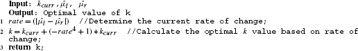

  

  AdjustForDataRate()

  Fig. 2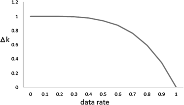

  

  Fine adjustment to k based on the data rate using the concave function

  Fig. 3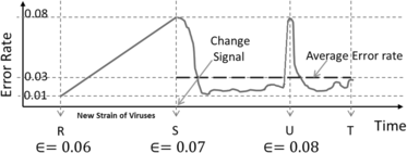

  

  Fine adjustment to k with variation of data rate based on a concave function

  Algorithm 3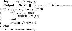

  

  GetDriftType()

  Algorithm 4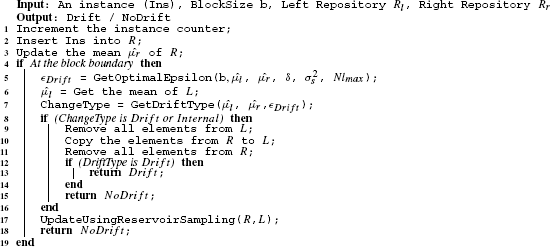

  

  SeqDrift2: IsDrift()

• 3. The final step involves hypothesis testing and updating the reservoir with instances from the right repository. The time complexity for the hypothesis testing operation is O(1) as no iteration through past instances is required. If the null hypothesis H ₀ holds true that no significant difference in means exist between the left and right repositories then the instances buffered in the right repository update the reservoir in the left repository. This update requires a single further pass through the instances in the right repository as it involves computing a random number in the range [1..n _l +1] (line 10 in Algorithm 5), and then determining whether an instance in the reservoir needs to be replaced (line 11).

  Algorithm 5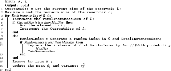

  

  UpdateUsingReservoirSampling()

Thus the first two steps have time complexity O(1), while the third step is also O(1) but requires a further scan through the right repository, thus making SeqDrift2 a two pass algorithm with respect to its internal buffer. The internal buffer is much more compact than the raw data as in a classification context the buffer consists of a bit stream as each data instance once classified will end up as a 0 for a correct classification or 1 in the case of a miss-classification. Also, in common with SeqDrift1, it is one-pass with respect to cut point examination, as it never reexamines previous cut points. We now state the following theorem to establish a theoretical guarantee on the false negative rate for the SeqDrift2 detector.

4.7 Compensating for repeated hypothesis testing in SeqDrift1 and SeqDrift2

The two SeqDrift methods presented both feature repeated hypothesis testing, in common with ADWIN and other concept change methods proposed in the literature. Repeated hypothesis testing carries with it the risk of increased type 1 errors, which in the concept change context is the increased risk of rejecting the null hypothesis H0 (that the means across the two data repositories are equal) when it is in fact true. The commonly adopted solution to this problem is to use the Bonferroni correction whereby the given δ value is divided by the number of hypotheses (n) tested since the last concept change point detected. However, the Bonferroni correction has been widely acknowledged to be too conservative in nature, by erring on the side of caution in setting the δ value too high and thus decreasing the sensitivity of the detection process. This is due to the fact the hypotheses tested in the change detection problem context are not independent of each other. Our motivation is to derive a less conservative correction factor and to give an expression for its update as each hypothesis test is carried out.

We consider a general scenario where n+1 blocks B ₁,B ₂,…,B _n ,B _n+1 (with mean values μ ₁,μ ₂,…,μ _n ,μ _n+1 respectively) have arrived at time point n+1 when n hypothesis tests have been carried out.

Theorem 5

The correction factor CF(n) to be used for the nth hypothesis test is given by:

$$ CF(n)=\frac{1}{\frac{1}{CF(n-1)}+\frac{1}{2^{n-1}}} $$

(16)

Proof

See Appendix 4 □

Thus, in our model the change significance level δ is scaled by the correction factor given by Theorem 5 to control the false positive probability. The correction factor computed by Theorem 5 is much less conservative than the Bonferroni correction and converges to $\frac {1}{2}$ for large values of n, as shown in the proof in Appendix 4.

5 Space, time and detection delay expectations

Before we undertake our empirical study on the five change detectors, namely SeqDrift1, SeqDrift2, ADWIN, PHT and EWMA we first summarize the space, time and detection delay complexities in Table 1. In order to provide easy reference to the methods named parameters have been used, as proposed by the authors of the methods concerned.

Table 1 Complexity analysis of change detectors

As shown in Table 1 PHT and EWMA are essentially memory less methods and are thus the most space efficient. The SeqDrift and ADWIN detectors store data instances in the detection window of size W. The latter uses compression in the form of an exponential histogram and is in general more space efficient than the SeqDrift detectors. The PHT, and EWMA detectors make a singe pass through the data, the SeqDrift detectors make two passes (one for buffering instances in the window and the other for updates), while ADWIN in the worst case makes O(logW) passes as it checks each possible combinations of cuts in its window. In the case of detection delay, PHT and EWMA have best case delays of 0 for the scenario that the change takes place at the first instance of the current block/grace period, as they check for changes with the arrival of each new instance whereas the SeqDrift detectors and ADWIN check in intervals of b (block size) and g (grace period) respectively.

On the basis of the above measures both PHT and EWMA are attractive but other measures such as false positive rate and actual processing times need to be evaluated empirically before final judgments can be made on the relative effectiveness of these different approaches.

6 Empirical study

Our Empirical study had five broad objectives. Firstly, we conducted a five-way comparative study between SeqDrift1, SeqDrift2, ADWIN, PHT and EWMA on the false positive rate by recording the number of false positives made on stationary data. Secondly, we tested the robustness of the detectors to noise by injecting data with varying amounts of noise and recording the number of changes flagged by each of the detectors. Thirdly, we subjected the detectors to abrupt changes and tested how far upstream changes were flagged by the detectors. We then tested the sensitivity of the change detectors by subjecting them to data that varied by different amounts over time and recorded the detection delay time and the processing time. Finally, we were interested in assessing the impact on classification accuracy, mining time and memory usage.

6.1 False positive rate assessment

This section elaborates the experimental procedure and the outcome in term of average false detection rates of SeqDrift1, SeqDrift2 and ADWIN.

6.1.1 Experimental setup

Our first experiment was designed to compare the false positive rates of the two SeqDrift detectors against ADWIN, Page Hinkley Test (PHT) and the Exponential Weighted Moving Average (EWMA) methods. We used a stationary Bernoulli distribution of 200,000 instances for this and tested the effect of various combinations of mean value (μ) and maximum allowable false positive rate (δ). For this experiment the block size for the SeqDrift detectors was set to the default value of 200 and ADWIN’s internal grace period parameter (the equivalent of the SeqDrift detector’s block size parameter) was also set to its default value of 32. In the case of PHT we set its internal parameters, drift level=10 and delta=0.02 to achieve a detection delay that was approximately equal to that of ADWIN and SeqDrift2 so that an assessment of its performance could then be on the basis of its false positive rate. In the case of EWMA we used a setting of its control parameters lamda=0.2, ARL ₀=1000 and warning level=0.1 that resulted in the lowest possible false positive rate. With this setting it turned out that its detection delay was similar to that of SeqDrift2, ADWIN, PHT thus enabling it to be compared with the others as well on the false positive rate. We used the implementations of PHT and EWMA from MOA Extensions by Paulo Mauricio Gonçalves Jr.¹

We conducted a total of 100 trials for each combination of μ and δ and the average false positive count for each combination was recorded for the three change detectors. In order to obtain statistically reliable results a separate Bernoulli stream segment was generated for each trial, with the statistical properties mentioned above.

6.1.2 Comparison of SeqDrift1, SeqDrift2 and ADWIN

We first report the comparison of SeqDrift with ADWIN as they both explicitly make use of a significance level δ and so the effects of this parameter can be assessed for the two different types of detectors. Figure 4 shows that all three detectors have good false positive rates that are substantially lower than the user defined maximum permissible level (δ) set. However, we observe that as the variance in the data increases with the increase in the μ value (for a Bernoulli distribution, the variance is μ×(1−μ)) the gap between ADWIN and the SeqDrift detectors widens. The ADWIN false positive rate increases progressively with the increase in variance as well as the lowering of confidence (i.e higher δ values). On the other hand the SeqDrift detectors retain a virtually zero false positive rate except when the confidence is low at 0.7 (δ=0.3), with SeqDrift1 and SeqDrift2 returning rates of .0028 %, compared to the ADWIN rate of .0128 % at μ=0.5. As the confidence becomes lower, the ϵ value decreases and this results in an increase in the false positive rate for ADWIN. The relatively higher false positive rate for ADWIN is due to the use of compression to reduce storage size of its buffer. ADWIN uses exponential histograms to compress its buffer and estimates true population means from the compressed version, thus introducing a degree of imprecision in the estimation of the population mean as explained in detail in Sect. 6.1.5. As the variance in the data increases so does the degree of imprecision in estimating the mean. In contrast, the SeqDrift detectors do not employ compression and estimate population means using random sampling techniques described in Sect. 4.

Fig. 4

Average false detections of SeqDrift1, SeqDrift2 and ADWIN

While both SeqDrift detectors exhibit better false positive rates than ADWIN, it is clear from Fig. 4 that SeqDrift1’s rate is better than that of SeqDrift2. This is to be expected as SeqDrift2 was specifically optimized for detection delay through the use of Algorithm 1, which trades off detection delay time with the false positive rate, while ensuring that the false positive rate does not rise above the user defined permissible rate of δ.

6.1.3 Overall assessment of false positive performance

Since ADWIN and the SeqDrift detectors use an explicit significance parameter it was necessary to choose a significance level for these detectors. We chose a level of 0.1 as levels below will be in favor of these detectors while a level of 0.3 would bias against them as the ϵ threshold for these detectors would then be too loose, thus increasing their false positive rate unfairly. Table 2 shows the average number of false positives recorded across the stable segment of the stream of length 200,000.

Table 2 Average false drift comparison across all chosen detectors

Table 2 shows that the false positive count for PHT and EWMA detectors is orders of magnitude higher than for the rest of the detectors. Such a high number of false positives would result in significant degradation of performance for classifiers using these two detectors, both in terms of computational time (to adjust models) and in terms of classifier accuracy (in wrongly restructuring existing accurate models). The results clearly show that the default behavior of these detectors in operating on a per instance basis is not desirable. A better performance from them can be expected when they check for drift in intervals, rather than individual instances. This will enable all detectors to be compared on an equal footing.

Table 3 shows that the gap between the (PHT, EWMA) pair and the rest has narrowed but it is clear that they have much higher false positive rates (except for PHT at mean 0.05) than the rest. Methods such as ADWIN and the SeqDrift detectors use detection thresholds that are specifically designed to minimize the false positive rate for a given significance level and this is the key reason for the difference in robustness of these methods.

Table 3 Average false positive rates across all chosen detectors

Interestingly, we observe that EWMA’s false positive rate for mean 0.3 is much smaller than its rate for mean 0.05 but the rate climbs very sharply for mean 0.5. We ran several more trials for EWMA but this trend was always observed, strongly suggesting that this is an inherent feature of the method, possibly due to increased precision in the Monte Carlo simulation for mean values around 0.3.

We decided to measure memory utilization across a stable stream as this represents the worst case scenario for methods such as the SeqDrift and ADWIN which are not memory less unlike PHT and EWMA. We suppressed false positives in order to eliminate the confounding effect of memory flushing by SeqDrift2 and ADWIN. As expected, PHT and EWMA had trivial memory consumption with 64 bytes and 48 bytes for PHT and EWMA respectively. For SeqDrift2 its memory consumption increased until its reservoir filled and then remained constant at 26 k (with a reservoir of size of 50,000), while for ADWIN it increased throughout and reached 2.8 K at the end of the 200,000 stream segment. We now carry forward the three detectors that had the best false positive rates, that is SeqDrift1, SeqDrift2 and ADWIN for further analysis.

6.1.4 Robustness to noisy data

This experiment was designed to test the robustness of the change detectors to noise. The higher the tolerance to noise, the more robust is the change detector. We simulated a noisy environment by introducing spikes in the error rate distribution that would typically arise from a classifier operating in a noisy environment. The key challenge was to sufficiently differentiate noise from the true signal so that noise could not be interpreted as true concept change. This was achieved by superimposing a distribution consisting of spikes on a stationary Bernoulli distribution.

The noise distribution was simulated by a Bernoulli distribution, but was sufficiently differentiated from the underlying stationary one by choosing a significantly higher population mean. We note that for a Bernoulli distribution its mean and variance are related by the expression σ ²=μ(1−μ), thus giving $\mu=\frac{(1-\sqrt{(}1-4\sigma^{2}))}{2}$. Thus, by introducing a factor k into the variance term σ ² we were able to compute the corresponding mean value,μ _n value required to generate new distributions that were sufficiently different from the stationary (base) distribution with mean μ _b that corresponds to a k value of 1. Different noise distributions were generated to test the effects of different levels of noise by varying k in the range 1 to 2.5 in increments of 0.1. We used a base mean value of 0.01 for the stationary signal (with k=1.0) which meant that the expected value of the variance was very low at 0.0099. For each value of k, 100 separate trials were conducted and the average false positive rate for the three change detectors were For each value of k, instances are drawn from a Bernoulli distribution with a mean value chosen at random between the base mean μ _b and μ _n .

As k increases, the variance of the noise signal increases and this has the effect of elongating the spike duration as well as the amplitude of the noise signal, as the noise trajectory for k=2.5 shows in Fig. 5. On the other hand the noise trajectory for k=1.5 is barely above that of the baseline value (with k=1.0), thus explaining why both ADWIN and SeqDrift detectors did not register an increase in the false positive rate.

Fig. 5

Effects of noise injection

Values of k in the range [1.0,1.6] yielded a zero false positive rate for all three detectors and so these entries were omitted from the results table. Table 4 shows that both SeqDrift1 and SeqDrift2 were very stable on noisy stream segments whereas ADWIN signaled a significant number of false positives when the level of noise increased. Given that noise is inevitable in most real world environments, this experiment clearly illustrates that both SeqDrift1 and SeqDrift2 are more robust to noise and hence better choices with respect to change detection. A comparison of ADWIN’s false positive rate for values of k in the range 2.0 to 2.5 reveals a significant increase, thus exposing a fundamental weakness of ADWIN to noisy data distributions containing spikes.

Table 4 Average drifts detected on a noisy stream

The underlying reasons for the higher tolerance of the SeqDrift detectors to noise are basically the same as for the experimentation with a pure stationary signal that we discussed in Sect. 6.1.2 above. The spikes in the noise signal have a much lower effect on the SeqDrift detector’s false positive rate as the data representing such spikes is very short-lived and is added in general to a much larger pool (the reservoir) from which it is smoothed through the use of the averaging process.

6.1.5 Flow-on effect of abrupt change on false positive rate

Abrupt changes are relatively easily detected by most change detectors in contrast to more gradual changes. When a sudden increase in the mean error rate for a classifier occurs its model needs to be updated to reflect such a change. However, if as a result of the sudden change the detector falsely signals further changes, then unnecessary overhead will be incurred by the classifier in performing updates to its model.

In order to test the vulnerability of the detectors to the flow on effects of abrupt changes we generated a Bernoulli stream of 100,000 instances with initial mean=0.01 and then another 100,000 instances were drawn from a distribution with an increased mean value. Thus, abrupt change was injected into the stream at the 100,000th instance and the concept changes flagged by each of the detectors were observed after processing the first 100,000 instances.

As Table 5 clearly shows ADWIN flags false changes upstream from its first detection point. For example, when the mean changes from the baseline value of 0.01 to 0.04, ADWIN first detects the change at point 100607 and then goes to flag 6 additional points further upstream from this point. In contrast, both SeqDrift detectors consistently report a single change point, with the exception of the less abrupt change scenario when a modest change was made to the mean from the 0.01 baseline to 0.02, for which no change was reported by either of the two detectors.

Table 5 Comparison of the drift detectors SeqDrift1, SeqDrift2 and ADWIN on an abrupt drift of various mean increments

As with the stationary distribution scenario the cause for false detections with ADWIN lies with its use of exponential histograms in approximating the true data distribution. In the case of abrupt shift, however the estimation error is much greater due to the speed of change. ADWIN approximates the state of a window segment by maintaining at most M buckets for a given value 2ⁱ, for integers i ranging from 0 upwards. In the case of an abrupt increase in the mean value of the data distribution, the probability of the appearance of 1 s is subject to rapid change due to increase in variance that accompanies an increase in the mean value. This rapid change in the frequency of 1 s in the stream causes the most recent buckets generated by ADWIN—i.e. buckets containing a single 1 to occur with widely different buckets lengths. This in turn causes the segments encapsulated by these buckets to have significantly different means, even when the underlying data distribution remains stationary after the change point. ADWIN stabilizes and stops detecting false change points only after a sufficient number of instances have been generated after the change point. When the number of buckets with value 1 exceeds the M threshold, merging of buckets occurs and sharp differences in mean values between buckets is smoothed due to the merging operation. Of course, a decrease in ADWIN’s M parameter will help to alleviate this problem, but as mentioned before this will come at a heavy price in terms of computational overheads.

Interestingly, ADWIN’s false alarms seem to disappear at the higher end of the μ range with no false positives reported for μ values 0.16 and greater. Although higher variability occurs in the data for such μ values, this is compensated by the increased frequency of the merge operation which is triggered by the higher frequency of 1 s in the stream that occur with distributions having higher mean values.

The SeqDrift detectors do not artificially slice the stream into discrete storage units but represent the entire window segment after the last cut point as one single storage unit for sampling and are thus in a better position to avoid errors arising from comparing units (buckets) of arbitrary and insufficient length to estimate mean values accurately.

6.2 Detection delays and false negative rate

In addition to the false positive rate, detection delay is an important performance measure as minimal delay in detecting changes will assist the classifier in responding to concept changes quickly.

In a high speed data stream environment another crucial performance factor is the processing speed of the change detector. A high processing time can lead to a bottleneck in the classifier, slowing down the speed with which it can classify instances. This is due to the fact that concept change detectors are invoked very often by the classifier (which for ADWIN will be 32 instances and for the SeqDrift detectors, every 200 instances). Each invocation requires the detector to compare means for one or more divisions of its buffer in its search for potential cut points. In general, the more extensive the search, i.e. the greater the number of candidates examined, the greater is the potential for detecting changes earlier but with a corresponding increase in processing time. In summary, a trade-off exists between detection delay and processing time. Given that the SeqDrift detectors and ADWIN have quite different change detection strategies it will be interesting to examine the trade-off in environments with different gradients of change.

The first experiment to compare the delays was designed in the following manner. A stationary Bernoulli data stream of different lengths 10000, 50000, 100,000 and 1,000,000 with mean=0.01(initial mean) were generated in separate trials. Different data lengths were used to ascertain the effects of history, if any.

With each data length, concept change was injected into the stream by generating the last 2300 instances with different gradients of change corresponding to 1×10⁻⁴, 2×10⁻⁴, 3×10⁻⁴ and 4×10⁻⁴. The processing time and the delay in detecting concept change injected were measured for each combination of data length and gradient of change. Each combination was repeated 100 times to boost reliability. In order to remove the confounding effect of reading time, the processing time measured only the actual time taken by the respective change detectors in executing their change detection algorithms.

ADWIN was used with its default grace period of 32, SeqDrift1 and SeqDrift2 with default block size of 200, and a significance level=0.01 was used for all three change detectors.

Figure 6, together with Table 6, clearly illustrates the detection delay versus processing time trade-off. In terms of processing time the two SeqDrift detectors were far superior to ADWIN. At the smallest data length of 10,000 ADWIN was around 3 times slower than SeqDrift1 and around 6 times lower than SeqDrift2. The gap between ADWIN and SeqDrift detectors widens as the data length increases: the processing speed of the SeqDrift detectors is essentially linear in data segment length while ADWIN is super-linear, as can be seen from the growth in processing times when the segment length is increased by factors of 10 and 100. This super-linear growth in ADWIN’s processing time is only to be expected as the number of hypotheses it tests is $n\frac{(n-1)}{2}$, versus n−1 for the SeqDrift detectors on a buffer of size n. Given that the processing time for the SeqDrift detectors start off at a much lower level than ADWIN and that the latter’s growth in time is super-linear in segment length, the SeqDrift detectors are by far the better choice for a high speed data stream environment.

Fig. 6

Detection delays of SeqDrift1, SeqDrift2 and ADWIN on streams with various slopes and lengths

Table 6 Processing times of SeqDrift1, SeqDrift2 and ADWIN on streams with different slopes and lengths

In terms of detection delay, however, it is clear from Fig. 6 that ADWIN has better mean detection delay when compared to the SeqDrift detectors. The SeqDrift detectors only examine a single candidate cut point for concept change that corresponds to the current boundary between the left and right repositories, whereas ADWIN examines all possible combinations of points in its buffer, and as such can be expected to detect change points sooner. As expected, the delay times reduced with increasing gradient of change, although we observe that the SeqDrift detector’s delay reduces at a faster rate than ADWIN with the gap closing for higher gradients of change. In terms of detection rate, all five detectors returned a value of 100 % for all combinations of data length and gradient of change.

We also observe from Fig. 6 and Table 6 that SeqDrift2’s detection delay times are much closer to that of ADWIN, PHT and EWMA than SeqDrift1, while maintaining a superior processing speed advantage. The slower speed of SeqDrift1 over SeqDrift2 is due to the fact that it requires $\frac{n_{l}}{b}$ passes through its left repository to perform sub-sampling, as opposed to two passes for the latter. On the other hand, SeqDrift2 does not use sub-samples but computes means across the two repositories in a one-pass incremental manner. In fact, SeqDrift2’s processing times are competitive with PHT and better than EWMA throughout the data length range. Despite the fact that EWMA is one pass, it has higher processing times than SeqDrift2 due to the large number of floating point calculations required in the computation of the control parameter L which is needed in flagging concept change.

Thus, from all the results examined so far we can conclude that SeqDrift2 is superior to SeqDrift1 as it maintains a competitive false positive rate to the latter while exhibiting superior detection delay and processing times. Henceforth in our experimentation we will focus exclusively on the SeqDrift2 and ADWIN change detectors.

6.3 Effects of reservoir sampling

In Sect. 6.2 we observed that replacing the sliding window by a reservoir in the implementation of the reference window reduces processing by around 50 %, as shown in Table 6. We now investigate another potential benefit of the reservoir which is improving sensitivity with respect to slowly varying data. We first generated data from a stationary Bernoulli distribution with mean 0.01 for 200,000 instances. Thereafter we injected concept change into the stream in two stages. In the first stage we injected change with a slope of 10⁻⁶ for the next 10,000 instances. This was followed by injecting change at a higher rate of 10⁻⁵ for the next 70,000 instances. This experiment models a real-world scenario where data is first in a stable state after detection of the previous concept change. Thereafter in stage 2, due to the emergence of a new concept, data is subject to a slow rate of change, followed by an increase in the rate of change after emergence of the new concept in stage 3. It would be of interest to investigate the effect of memory retention of the oldest data samples from stage 1 on detection sensitivity measures. The performance measures of interest here are the detection rate, detection delay, stability of detection, as measured by the standard deviation of the detection delay over the 100 trials conducted, and the memory retention capacity of each of the two memory management schemes.

Table 7 shows that with reference windows of size 5,000 and 10,000 the reservoir scheme significantly outperformed the sliding window scheme on all measures. When the window size is less than 10,000 the sliding window approach was unable to store any samples from the oldest (stage 1) state and its buffer consisted entirely of samples from stage 2 and stage 3 thus severely affecting its sensitivity, causing it to return an average detection delay time which are 3.34 and 1.84 times that of the reservoir for sizes 5000 and 10,000 respectively. Furthermore, its detection behavior is highly unstable as the corresponding standard deviations of its detection times are 12.58 and 6.9 times that of the reservoir approach. However, as the reference window size increases the sensitivity of the sliding window approach improves and converges to that of the reservoir at around the 40–50,000 window size setting. As expected, Table 7 also shows that the relative performances of the two approaches is highly correlated to the memory retention capacity which is the percentage of data samples retained from the original stable state (stage 1). In a real world setting the length of concept formation (the sum of stage 2 and stage 3 lengths) may be much greater than memory available in the reference window and in such situations the reservoir approach is by far the superior choice.

Table 7 Sensitivity of reservoir over sliding window approach

6.4 Effects of detection thresholds and window management strategies

Given that SeqDrift2 had the best false positive performance and that ADWIN maintains a good balance between detection delay and false positive rate it is of interest to examine whether each of these two best performing methods can benefit from using features implemented in each other.

Table 8 shows clearly that neither of the two change detectors benefit from using each other’s features. When ADWIN uses SeqDrift2’s detection threshold its false positive rate increased (measured for mean 0.3 and δ=0.1) while only a very marginal improvement resulted for detection delay (measured for slope 1×(10)⁻⁴). The opposite was observed when SeqDrift2 used ADWIN’s threshold: its false positive decreased marginally but its detection delay increased quite considerably, showing that SeqDrift2’s detection threshold is more sensitive than that of ADWIN. Unlike SeqDrift2, ADWIN cannot benefit from SeqDrift2’s more sensitive detection threshold as it maintains multiple cut points in its window thus contributing to an increased false positive rate. These results are not unexpected as each of the two change detectors are optimized to work with their own detection thresholds.

Table 8 Further Experimentation on SeqDrift2 and ADWIN

The third experiment showed once again the effectiveness of the reservoir sampling strategy. Replacement of the reservoir with a buffer that grows in an unbounded fashion led to a very marginal improvement in detection delay while increasing the false positive rate. It should be noted that an unbounded buffer may be impractical in many situations as in a stable stream segment of large size the left repository could exceed the memory available. Apart from that the computational cost of sampling the left repository would also increase considerably.

The final experiment with ADWIN operating on a single cut point does not yield any clear material benefits: although its false positive rate decreased quite considerably its detection delay increased sharply yielding values that were much higher than SeqDrift2 Thus the overall conclusion is that each of the two change detectors are best served by keeping them in their default configurations with their native detection thresholds.

6.5 Integration with adaptive Hoeffding tree classifier

In a typical data stream environment, a change detector operates in conjunction with a classifier. To the extent that a change detector is able to detect concept changes efficiently in the minimal possible time with the least number of false detections, it will support the classifier in processing the data stream quicker and return higher classification accuracy. To investigate this premise we next integrated SeqDrift2 and ADWIN with the Hoeffding Adaptive Decision tree (Bifet and Gavaldà 2009) and conducted a series of experiments on datasets generated with various different stream generators, sea concepts² and the real world data sets, airline and poker hand.³ For the synthetic data the degree of concept change was controlled by specifying the number of features (f) that were subject to change. More details of the characteristics of these data generators is available from Bifet et al. (2010).

For each experiment we track four performance measures: classification time, classification accuracy, the Kappa statistic and memory, measured in terms of tree size. These statistics represent averages gathered at intervals of 10,000 instances.

Table 9 shows that SeqDrift2 clearly outperforms ADWIN in terms of all four measures that we tracked. In terms of classification accuracy, SeqDrift2 was better in 10 out of 11 experiments conducted. In the experimentation with the rotating hyperplane (with 6 drifting attributes) substantial improvements in accuracy of around 5 % or greater was achieved. We attribute SeqDrift2’s better accuracy to its superior false positive rate. When detections are signaled at a given node in the tree, the sub-tree rooted at that node is removed as it is thought to represent an old or outdated concept. If the detection is false, then the removal of the sub-tree will reduce accuracy as the concept it represents is actually current. Given that ADWIN registers a higher false positive rate than SeqDrift2 in general, the incidence of erroneous pruning will be proportionately higher than in SeqDrift2, thus resulting in a lower accuracy. The learning curves given in Fig. 7 support this line of reasoning. The learning curves in Fig. 7 were generated using the holdout evaluation method in MOA (Bifet et al. 2010) and represents 3 of the 11 datasets used. The curves for the rest follow the same trends and have been omitted to conserve space.

Fig. 7

Variation of accuracy with training set size

Table 9 Integration of Change Detectors with Adaptive Hoeffding Tree. A—Accuracy, T—Mining Time, K—Kappa coefficient, N—Total number of nodes and L—Number of leaf nodes

As Fig. 7 shows, the learning curves for ADWIN fluctuate significantly throughout the range of training set size. In contrast, SeqDrift2’s curves are smoother and behave closer to the ideal scenario of smooth incremental growth in accuracy with increasing training set size.

The improvements in classification accuracy for SeqDrift2 are closely mirrored by improvements in Kappa value. The Kappa statistic for a given classifier measures the degree of improvement of the classification decisions over pure chance. SeqDrift2’s Kappa values are consistently greater than that of ADWIN (with the exception of the Poker Hand dataset), thus inspiring greater confidence that the decisions taken with it in operation are better than chance.

The most significant improvements in performance for SeqDrift2, however, occur in the area of classification time. In some cases the mining time more than halved with the use of SeqDrift2 in place of ADWIN. The major reason for this reduction in time is due to SeqDrift2’s efficient change detection strategy that employs a single forward sequential scan of its memory buffer instead of repeated backward scans and checks for cut points at every bucket boundary, as ADWIN does.

Finally, we note that SeqDrift2’s induced smaller trees than ADWIN in 8 of 11 cases that we considered. As with accuracy the major cause for higher memory utilization with ADWIN as the change detector is its higher false positive rate. When a sub-tree is pruned as a result of concept change being signaled, a new alternate sub-tree is grown and maintained.

7 Discussion, conclusion and future work

In this research we have presented a novel scheme for concept change detection that employs a sequential one pass strategy. Our results show that overall, our change detection approach outperformed ADWIN with respect to false positive rate and processing time, while maintaining competitive detection delay times. The gain in processing time over ADWIN was undoubtedly due to the sequential hypothesis testing strategy used. Sequential hypothesis testing meant that alternate cut points further downstream than the current block need never be re-examined, thus ensuring that processing overheads were held to a minimum.

Our results also showed that our change detectors also significantly outperformed the Page Hinkley detector with respect to false positive rate while maintaining competitive processing and detection delay times. Reservoir sampling was the key to the success of SeqDrift2 with respect to achieving low false positive rates and low detection times. The use of the reservoir enabled SeqDrift2 to keep a representative sample of the data from the stream without relying on data compression/data aggregation strategy such as used by ADWIN that causes the latter to return higher false positive rates

Apart from the use of the reservoir to improve performance, reservoir sampling is also an ideal solution to the load problems caused by ultra high speed data streams. Given any classifier, there will always be some environment or some data stream that produces instances at a faster rate than it can cope with. In such cases the classifier will end up losing valuable data and its accuracy could be severely impacted over a period of time if the stream is subjected to change. Reservoir sampling in this case can be used to reduce information loss by feeding the classifier with a representative sample of the data produced by the stream. In this context both the classifier and concept change detector could operate under a single unified data input supply mechanism. A reservoir sample of the raw stream data would be first presented to the classifier for training purposes and its processed binary output in terms of classification decisions then input to a separate reservoir maintained for change detection purposes.

Our future work in this area will consist of integrating the process of optimizing the false positive and false negative rates. Currently our strategy is a two phased one, whereby in Phase 1 we obtain an ϵ cut value that minimizes the false positive rate. In Phase 2, we optimize for detection delay by relaxing (i.e reducing) the ϵ cut threshold value (Algorithm 1), subject to the constraint that the estimated false positive rate is no bigger than the user desired false positive rate,δ. Though this process helps to improve detection delay time for SeqDrift2, it lacks flexibility in the sense that the user cannot prioritize false positive rate over detection delay and vice versa. Ideally, the user should be able to guide the change detection process by specifying weights for the false positive rate and detection delay. In order to implement this process we propose that a composite function f of the form: w _fp δ′+w _dd delay _i+1 be minimized, where w _fp ,w _dd denote the weights for the false positive rate and detection delay time respectively; δ′ is the empirical false positive rate as formulated in Sect. 4.3; and delay _i+1 denotes the estimated detection delay when the (i+1)th block has been received, extrapolated via some form of regression function from the i blocks received since the last detection point.

Appendices

Appendix 1: Proof of Theorem 3

$$\begin{aligned} &\Pr\bigl(2|\mu_l-\mu_r| \le2\epsilon\bigr)=\Pr\bigl(| \mu_l-\hat{\mu_l}+\hat{\mu_l}-\mu _r+\mu_l-\hat{\mu_r}+\hat{\mu_r}- \mu_r|\le2\epsilon\bigr) \\ &\quad =\Pr \bigl(|\mu_l-\hat{\mu_l}+\hat{ \mu_l}-\mu_r+\mu_l-\hat{\mu_r}+ \hat{\mu _r}-\mu_r| \le k\epsilon+(1-k)\epsilon+k \epsilon+(1-k)\epsilon \bigr) \\ &\quad {}=\Pr\bigl(\bigl(|\mu_l-\hat{\mu_l}|\le k\epsilon\bigr)+\Pr\bigl|( \mu_l-\hat{\mu_r})\bigr|\le (1-k)\epsilon\bigr) \\ &\qquad {}+\Pr\bigl(|\mu_l-\hat{\mu_r}|\le k\epsilon\bigr)+\Pr\bigl(| \mu_r-\hat{\mu _r}|\bigr)\le(1-k)\epsilon \ \mbox{for some}\ k \in(0,1) \end{aligned}$$

From the union bound we have: $\Pr(|\hat{\mu_{l}}-\hat{\mu_{r}}| \le\epsilon) \le \Pr(|\mu_{l}-\hat{\mu _{l}}|\le k\epsilon)+\Pr(|\mu_{l}-\hat{\mu_{r}}|)\le(1-k)\epsilon$ and $\Pr(|\hat{\mu_{l}}-\hat{\mu_{r}}| \le\epsilon) \le \Pr(|\mu_{l}-\hat{\mu _{r}}|\le k\epsilon)+\Pr(|\mu_{r}-\hat{\mu_{r}}|\le(1-k)\epsilon)$.

But from our starting assumption, we have$:\Pr(|\hat{\mu_{l}} - \hat{\mu _{r}}| \le\epsilon)>1-\delta$.

Thus $\Pr(2|\mu_{l}-\mu_{r}|\le2\epsilon)>2\Pr(|\hat{\mu_{l}}-\hat{\mu_{r}}| \le \epsilon) >2(1-\delta)$, or in other words:Pr(|μ _l −μ _r |≤2ϵ)>(1−δ)which leads to a contradiction since Pr(|μ _l −μ _r |>2ϵ) with probability 1.

Thus our assumption of $\Pr(|\hat{\mu_{l}} - \hat{\mu_{r}}| \leq\epsilon ) >1-\delta$ is false and so $\Pr(|\hat{\mu_{l}} - \hat{\mu_{r}}| > \epsilon) >1-\delta$ which means that the probability of a false negative is <δ, which in turn proves the theorem.

Appendix 2: Proof of Lemma 1

$\frac{\epsilon_{i-1} - \epsilon_{i}}{\epsilon_{i-1}} < t$ can be rewritten as$:\frac{\epsilon_{i-1}}{\epsilon_{i}} < \frac{1}{1-t}$.

From Eq. (12), we have:

$$ \epsilon_{i-1} = \frac{\alpha_{i-1}}{3n_{r}(1-k_{i-1})} $$

(17)

and

$$ \epsilon_{i} = \frac{\alpha_{i}}{3n_{r}(1-k_{i})} $$

(18)

where $\alpha_{i-1} = (\ln (\frac{4}{\delta'_{i-1}} )+\sqrt {\ln (\frac{4}{\delta'_{i-1}} )^{2} + 18\sigma_{s}^{2}n_{r}\ln (\frac{4}{\delta'_{i-1}}} ) )$ and $\alpha_{i} = (\ln (\frac{4}{\delta'_{i}} )+ \sqrt{\ln (\frac{4}{\delta'_{i}} )^{2} + 18\sigma_{s}^{2}n_{r}\ln (\frac{4}{\delta'_{i}}} ) )$ where $\delta'_{i-1}$, $\delta'_{i}$ are the estimated false positive rates associated with iterations i−1 and i respectively.

Dividing Eq. (16) by Eq. (17) yields,

$$ \frac{\epsilon_{i-1}}{\epsilon_{i}} = \frac {(1-k_{i})}{(1-k_{i-1})}*\frac{\alpha_{i-1}}{\alpha_{i}} $$

(19)

Rearranging Eq. (18),

$$ \frac{\alpha_{i-1}}{\alpha_{i}} = \frac{(1-k_{i-1})}{(1-k_{i})}*\frac {\epsilon_{i-1}}{\epsilon_{i}} $$

(20)

Now $\frac{(1-k_{i-1})}{(1-k_{i})} <1$ as $k_{i-1}=\frac{1}{f}k_{i} \Rightarrow k_{i-1} > k_{i}$.

Thus from Eq. (19) and expression (14) we get$,\frac{\alpha_{i-1} - \alpha_{i}}{\alpha_{i-1}} < t$ which in turn means that $\frac{\delta'_{i} -\delta'_{i-1}}{\delta'_{i-1}} < t$, thus proving the lemma.

Appendix 3: Proof of Theorem 4

Denote ϵ ₁ as the cut threshold used at the first iteration with k=k ₁=0.5. Now ϵ ₁ is given by$:\epsilon_{1}=\frac {1}{3(1-0.5)n_{r}} (p+\sqrt{p^{2}+18\sigma_{s}^{2}n_{r}p} )$ and $\epsilon_{2}=\frac{1}{3(1-k_{2})n_{r}} (p+\sqrt{p^{2}+18\sigma _{s}^{2}n_{r}p} )$. Thus $\epsilon_{2}=\frac{1}{2} (\frac {1}{(1-k_{2})} )\epsilon_{1}$. Generalizing the derivation of ϵ to the (i−1)th iteration yields:

$$\begin{aligned} \epsilon_i=\frac{1}{2} \biggl(\frac{1}{(1-k_i)} \biggr) \epsilon_1 \end{aligned}$$

(21)

From (12) we have

$$\begin{aligned} \epsilon_{i-1}=\frac{1}{3(1-k_{i-1})n_r} \Bigl(p+\sqrt{p^2+18 \sigma _{s}^2n_rp} \,\Bigr) \end{aligned}$$

(22)

Applying the result from Lemma 1 on Eqs. (18) and (19), we obtain the following quadratic:

$$ 3{\epsilon_1}^2n_rq^2-4(1-t) \epsilon_1pq-24(1-t)\sigma_{s}^2p=0 $$

(23)

where $q=\frac{(1-k_{i-1})}{(1-k_{i})}$ and t is the tolerance factor.

Equation (22) when solved yields

$$ q=\frac{(1-t)(2p+\sqrt{(4p^2+72n_r\sigma_{s}^2p)}}{3\epsilon_1n_r} $$

(24)

We thus have:

$$ \frac{(1-k_{i-1})}{(1-k_i)}=\frac{(2p+\sqrt{(4p^2+72n_r\sigma _{s}^2p)}}{3\epsilon_1n_r} $$

(25)

We also have $k_{i-1}=\frac{1}{k}k_{i}=0.5f^{i-2}$.

Substituting for k _i−1 and k _i in (24) above and replacing the right hand side of (24) by q for simplicity, gives:

$$ \frac{1-f0.5^{i-2}}{1-0.5^{i-2}}=q $$

(26)

which when solved yields:

$$ i=2+\log_f \biggl(2\frac{(q-1)}{(q-f)} \biggr) $$

(27)

Equation (26) shows that the number of iterations i in which Algorithm 1 converges is logarithmic (to base f) in q, and combined with Eq. (22) which expresses q as a square root function of $\sigma_{s}^{2}$, we conclude that i is a logarithmic function (to base f) of $\sigma_{s}^{2}$. With respect to δ, i is logarithmic (again with base f) with respect to p, which in turn is inverse logarithmic (to base e) with respect to δ. Thus overall, with adjustment of logarithmic bases we have $i = O(\log(\log(\frac{1}{\delta})))$.

With a f value of 0.75, a p value of 5.99 (corresponding to a δ value of 0.01), a $\sigma_{s}^{2}$ value of 0.2, and n _r =200, the use of (25) and (22) yields convergence at the 20th iteration which corresponds to δ′=0.0099 (see Table 10) which is very close to the desired value of 0.01. Using the same f value of 0.75, and p value of 5.99, a $\sigma_{s}^{2}$ value of 0.02, and n _r =200, convergence was signaled by (25) and (22) at the 18th iteration, corresponding to δ′ value of 0.0099 (see Table 10) which again is very close to the desired value of 0.01.

Table 10 Optimization of k value by Algorithm 1

Although we used a value of 0.75 for f in Algorithm 1 (line 5), in principle other values such as 0.8 or 0.9 can be used to produce very similar results. We experimented with different values of f and found that the difference in results is insignificant. Even an extreme value for f of 0.1 yields an ϵ value of 0.1199 (very similar to the 0.1202 value achieved with f=0.75) at convergence for the high variance case, a very similar result to the one that we achieved with f=0.75. The same holds true for the low variance case; with f=0.1, convergence was achieved with an ϵ value of 0.0460 (again, very similar to the 0.0461 achieved with f=0.75. We can thus conclude that the optimization process is not sensitive to the value of f used, provided that a reasonable value for f is used, say in the range [0.1,0.9]. Table 10 clearly shows the utility of the optimization process. In the high variance scenario the ϵ value starts off at a high value of approximately 0.24 for an equal-sized data repository configuration and decreases by around 0.12 at the point of convergence (we say that convergence is achieved when the difference between consecutive δ′ values is less than or equal to 0.0001, a tolerance factor) to reach a value of 0.1202, thus greatly increasing sensitivity while ensuring that the false positive rate is kept within user-defined bounds. A similar behavior is observed for the low variance case, although the reduction in the ϵ value at 0.045 is not so drastic in absolute terms. As expected, the ϵ values at convergence are very much different from each other, as the determination of ϵ is dominated by the variance term, as shown in Eq. (12).

Appendix 4: Proof of Theorem 5

In the first test (1) on |μ ₂−μ ₁| on B ₁, B ₂ boundary, the false positive error resulting from a cut is δ′=δ. In the second test (2), there are three cases to consider.

Case (1) corresponds to the case when no cut was made on the B ₁, B ₂ boundary. This case does not contribute to a false positive error rate and hence can be ignored.

Case (2) arises when a cut was made on the B ₁, B ₂ boundary and when $|\frac{\mu_{1} + \mu_{2}}{2} - \mu_{3}| > |\mu_{3} - \mu_{2}|$. It can be seen that Case (2) does not contribute to the false positive rate as the cut made on the B ₁, B ₂ boundary has ensured that a reduction in the mean difference |μ ₃−μ ₂| between the two samples used in the second hypothesis test. This is due to the fact that $|\frac{\mu_{1} + \mu_{2}}{2} - \mu_{3}| > |\mu_{3} - \mu_{2}|$.

We now consider Case (3) which corresponds to the situation where a cut was made on the B ₁, B ₂ boundary and $|\frac{\mu_{1} + \mu_{2}}{2} - \mu_{3}| < |\mu_{3} - \mu_{2}|$. This case increases the false positive rate. We now estimate the degree of increase by enumerating the fraction of all possible scenarios possible with the arrival of 3 blocks in the stream.

With the arrival of 3 blocks there are a total of 6 possible orderings for μ ₁, μ ₂ and μ ₃. These orderings are (in ascending order of value):(μ ₁,μ ₂,μ ₃), (μ ₁,μ ₃,μ ₂), (μ ₂,μ ₁,μ ₃), (μ ₂,μ ₃,μ ₁), (μ ₃,μ ₁,μ ₂), (μ ₃,μ ₂,μ ₁). Out of these exactly half (3 out of 6) cause an increase of |μ ₃−μ ₂| over $|\frac{\mu_{1} + \mu_{2}}{2} - \mu_{3}|$, and thus contribute to the increase in the false positive rate.

With an assumption of uniformity (equal priors in the general case) of the probability of occurrence of these 6 triples we can infer that the false positive error δ in test (1) has contributed an amount $\frac{\delta}{2}$ to the false positive error in test (2), thus giving an overall false positive error of $\delta+\frac{\delta}{2}$ and a correction factor CF(1) of $\frac{2}{3}$ to be applied.

Generalizing this situation to test (3) we have an overall false positive error at this test of $\delta+ \frac{\delta+ \frac{\delta }{2}}{2} = \delta+ \frac{\delta}{2}+\frac{\delta}{4}$ and a correction factor CF(2) of $\frac{4}{7}$ which is $\frac{\delta}{\frac {1}{CF(1)}+\frac{1}{4}}$. Thus, in general after n hypothesis tests the false positive error is$:\delta+ \frac{\delta}{2}+\frac{\delta }{4}+\cdots+\frac{\delta}{2^{n-1}}$. and the CF(t) to be applied is:

$$\begin{aligned} CF(n)=\frac{1}{\frac{1}{CF(n-1)}+\frac{1}{2^{n-1}}} \end{aligned}$$

(28)

which proves the theorem.

We observe that the correction factor computed above is much less conservative than the Bonferroni correction and converges to $\frac {1}{2}$ for large values of n.

References

Aggarwal, C. C., Han, J., Wang, J., & Yu, P. S. (2003). A framework for clustering evolving data streams. In VLDB endowment, VLDB ’03: Vol. 29. Proceedings of the 29th international conference on very large data bases (pp. 81–92).
Audibert, J. Y., Munos, R., & Szepesvári, C. (2007). Tuning bandit algorithms in stochastic environments. In Proceedings of the 18th international conference on algorithmic learning theory, ALT’07 (pp. 150–165). Berlin, Heidelberg: Springer.
Basseville, M., & Nikiforov, I. V. (1993). Detection of abrupt changes: theory and application. Upper Saddle River: Prentice-Hall.
Bernstein, S. N. (1946). The theory of probabilities. Moscow, Leningrad: Gostekhizdat.
Bifet, A., & Gavaldà, R. (2007). Learning from time-changing data with adaptive windowing. In Proceedings of the seventh SIAM international conference on data mining. Philadelphia: SIAM.
Bifet, A., & Gavaldà, R. (2009). Adaptive learning from evolving data streams. In Lecture notes in computer science: Vol. 5772. Advances in intelligent data analysis VIII (pp. 249–260). Berlin, Heidelberg: Springer.
Bifet, A., Holmes, G., Kirkby, R., & Pfahringer, B. (2010). MOA: massive online analysis. Journal of Machine Learning Research, 11, 1601–1604.
Borne, K. D. (2007). A machine learning classification broker for petascale mining of large-scale astronomy sky survey databases. In Next generation of data mining and cyber-enabled discovery for innovation (NGDM07). Baltimore: National Science Foundation.
Das, K., Sug, K. B., Giannella, C., & Kargupta, H. (2009). Scalable distributed change detection from astronomy data streams using local, asynchronous eigen monitoring algorithms. In SIAM international conference on data mining (SDM’09), Nevada (pp. 156–245). Philadelphia: SIAM.
Gama, J. (2010). Knowledge discovery from data streams (data mining and knowledge discovery series). Chapman and Hall/CRC data mining and knowledge discovery series. Minneapolis: CRC Press.
Gama, J., Medas, P., Castillo, G., & Rodrigues, P. P. (2004). Learning with drift detection. In Lecture notes in computer science: Vol. 3171. Proceedings of the 17th Brazilian symposium on artificial intelligence (Advances in artificial intelligence—SBIA 2004) (pp. 286–295). Berlin: Springer.
Ho, S. S. (2005). A martingale framework for concept change detection in time-varying data streams. In Proceedings of the 22nd international conference on machine learning, ICML ’05 (pp. 321–327). New York: ACM.
Hoeglinger, S., & Pears, R. (2007). Use of Hoeffding trees in concept based data stream mining. In Third international conference on information and automation for sustainability, ICIAFS 2007 (pp. 57–62). New York: IEEE Press.
Hoeglinger, S., Pears, R., & Koh, Y. S. (2009). CBDT: a concept based approach to data stream mining. In Proceedings of the 13th Pacific-Asia conference on advances in knowledge discovery and data mining, PAKDD ’09 (pp. 1006–1012). Berlin, Heidelberg: Springer.
Hulten, G., Spencer, L., & Domingos, P. (2001). Mining time-changing data streams. In Proceedings of the seventh ACM SIGKDD international conference on knowledge discovery and data mining, KDD ’01, (pp. 97–106). New York: ACM.
Jose, M. B., Campo-Ávila, J. D., Fidalgo, R., Bifet, A., Gavaldà, R., & Morales-bueno, R. (2006). Early drift detection method. In Proceedings of the 4th ECML PKDD int. workshop on knowledge discovery from data streams, Berlin (pp. 77–86).
Kifer, D., Ben-David, S., & Gehrke, J. (2004). Detecting change in data streams. In Proceedings of the thirtieth international conference on very large data bases, VLDB endowment, VLDB ’04 (Vol. 30, pp. 180–191).
Klinkenberg, R., & Joachims, T. (2000). Detecting concept drift with support vector machines. In Proceedings of the seventeenth international conference on machine learning, ICML ’00 (pp. 487–494). San Francisco: Morgan Kaufmann.
Kuncheva, L. I. (2013). Change detection in streaming multivariate data using likelihood detectors. IEEE Transactions on Knowledge and Data Engineering, 25(5), 1175–1180.
Maurer, A., & Pontil, M. (2009). Empirical Bernstein bounds and sample-variance penalization. In The 22nd conference on learning theory, COLT 2009.
Mnih, V., Szepesvári, C., & Audibert, J. Y. (2008). Empirical Bernstein stopping. In Proceedings of the 25th international conference on machine learning, ICML ’08 (pp. 672–679). New York: ACM.
Nishida, K., & Yamauchi, K. (2007). Detecting concept drift using statistical testing. In Proceedings of the 10th international conference on discovery science, DS’07 (pp. 264–269). Berlin, Heidelberg: Springer.
Page, E. S. (1954). Continuous inspection schemes. Biometrika, 41(1/2), 100–115.
Ross, G. J., Adams, N. M., Tasoulis, D. K., & Hand, D. J. (2012). Exponentially weighted moving average charts for detecting concept drift. Pattern Recognition Letters, 33(2), 191–198.
Sakthithasan, S., Pears, R., & Koh, Y. S. (2013). One pass concept change detection for data streams. In Lecture notes in computer science: Vol. 7819. Advances in knowledge discovery and data mining (pp. 461–472). Berlin, Heidelberg: Springer.
Sebastiao, R., & Gama, J. (2009). A study on change detection methods. In Proceedings of the 14th Portuguese conference on artificial intelligence, EPIA 2009 (pp. 353–364). Berlin, Heidelberg: Springer.
Shivaswamy, P. K., & Jebara, T. (2010). Empirical Bernstein boosting. In JMLR.org, JMLR proceedings: Vol. 9. Proceedings of the 13th international conference on artificial intelligence and statistics (AISTATS) (pp. 733–740).
Vitter, J. S. (1985). Random sampling with a reservoir. ACM Transactions on Mathematical Software, 11(1), 37–57.
Widiputra, H., Pears, R., & Kasabov, N. (2011). Multiple time-series prediction through multiple time-series relationships profiling and clustered recurring trends. In Lecture Notes in Computer Science: Vol. 6635. Advances in knowledge discovery and data mining (pp. 161–172). Berlin, Heidelberg: Springer.
Author information
Authors and Affiliations
Corresponding author
Additional information
Editor: Joao Gama.